Article

Large-Scale Populus euphratica Distribution Mapping Using Time-Series Sentinel-1/2 Data in Google Earth Engine

1
Aerospace Information Research Institute, Chinese Academy of Sciences, Beijing 100094, China
2
University of Chinese Academy of Sciences, Beijing 100049, China
3
Key Laboratory of Earth Observation of Hainan Province, Hainan Research Institute, Aerospace Information Research Institute, Chinese Academy of Sciences, Sanya 572029, China
*
Author to whom correspondence should be addressed.
Remote Sens. 2023, 15(6), 1585; https://doi.org/10.3390/rs15061585
Submission received: 26 January 2023 / Revised: 8 March 2023 / Accepted: 12 March 2023 / Published: 14 March 2023
(This article belongs to the Special Issue Image Analysis for Forest Environmental Monitoring)

Abstract

:
Accurate and efficient large-scale mapping of P. euphratica distribution is of great importance for managing and protecting P. euphratica forests, policy making, and realizing sustainable development goals in the ecological environments of desert areas. In large regions, numerous types of vegetation exhibit spectral characteristics that closely resemble those of P. euphratica, such as Tamarix, artificial forests, and allée trees, posing challenges for the accurate identification of P. euphratica. To solve this issue, this paper presents a method for large-scale P. euphratica distribution mapping. The geographical distribution characteristics of P. euphratica were first utilized to rapidly locate the appropriate region of interest and to further reduce background complexity and interference from other similar objects. Spectral features, indices, phenological features, and backscattering features extracted from all the available Sentinel-2 MSI and Sentinel-1 SAR data from 2021 were regarded as the input for a random forest model used to classify P. euphratica in the GEE platform. The results were then compared with the results from the method using only spectral features and index features, the results from the method that only added phenological features, and the results from the method that added phenological features and backscattering features by visually and quantitatively referencing field-surveyed samples, UAV data, and high-spatial-resolution data from Google Earth Data and Map World. The comparison indicated that the proposed method, which adds both phenological and time-series backscattering features, could correctly distinguish P. euphratica from other types of vegetation that have spectral information similar to P. euphratica. The rates of omission errors (OEs), commission errors (CEs), and overall accuracy (OA) for the proposed method were 12.53%, 11.01%, and 89.32%, respectively, representing increases of approximately 9%, 17%, and 13% in comparison with the method using only spectral and index features. The proposed method significantly improved the accuracy of P. euphratica classification in terms of both omission and, especially, commission.

1. Introduction

Populus euphratica is a valuable germplasm resource in the oasis ecological zones of semi-arid and arid desert areas, and it plays an irreplaceable role in maintaining ecological balance in desert regions [1,2]. Accurate and efficient large-scale mapping of P. euphratica distribution is of great importance for management and protection, policy making, and realization of sustainable development goals in the ecological environments of desert areas. Remote sensing techniques can be used to macroscopically and visually observe the distribution of P. euphratica, so these techniques are the principal ways of mapping large-scale P. euphratica distribution. Previous studies on P. euphratica recognition based on remote sensing techniques mainly focused on small regions [3,4,5,6]. Su et al. used airborne hyperspectral data to classify land cover in the Ejin Banner oasis, where the forest is dominated by P. euphratica [7]. Li et al. extracted the distribution of P. euphratica in the Daliyabui oasis in the hinterland of the Taklimakan Desert from Sentinel-2 data [6]. Peng et al. used multisource remote sensing images to extract P. euphratica distribution in the Tarim National Nature Reserve [2]. However, there are few studies on large-scale P. euphratica distribution mapping. Due to the diversity of tree species in large regions, there are many instances where different objects have the same spectrum or the same objects have different spectra, as happens in the present case with P. euphratica, Tamarix, artificial forests, and allée trees [6]. Therefore, the main difficulty in accurately extracting P. euphratica distribution in a large area is that the spectra are so similar among these different types of vegetation that it is hard to recognize P. euphratica accurately by depending only on the spectra, texture, and orientation features.
Aiming to resolve this issue, we first applied the perspective of human cognition to remote sensing. The basis of human recognition of specific objects is usually a combination of the features of remote sensing images with geographic features and expert experience. P. euphratica mainly grows along riparian zones with a corridor distribution. Therefore, its geographic distribution features can be used to rapidly locate the growing areas of P. euphratica and, thus, improve the efficiency and accuracy of P. euphratica recognition. Secondly, vegetation phenology is widely used to improve classification accuracy due to its unique characteristics [8,9,10,11], especially in crop classification [10,11,12]. Liu et al. introduced crop phenology derived from Sentinel-2 NDVI time-series data to map large-scale crops precisely and found that the classification results were improved [11]. Pan et al. applied the crop proportion phenology index [13] to estimate the planting area for winter wheat in Tongzhou and Shuyang based on time-series MODIS EVI data, and the results revealed that combining crop phenological features can facilitate agricultural monitoring and mapping [13]. It is well-known that phenology based on remote sensing technology generally employs vegetation indices extracted from medium- and low-spatial-resolution remote sensing data with a high temporal resolution; e.g., MODIS, the Landsat series, or Sentinel-2 [14,15,16,17]. Therefore, some researchers have discussed the accuracy of phenological findings derived from different vegetation indices. Experiments suggest that phenological findings derived from the enhanced vegetation index (EVI) time-series data are more realistic and accurate [17,18,19]. Kowalski et al. found that a phenology map produced using the EVI performed better than the results from the normalized difference vegetation index (NDVI) based on Landsat and Sentinel-2 data in temperate broadleaf forests [18]. Descals et al. (2020) discovered that the phenological results derived from time-series Sentinel-2 EVI data were more accurate than those estimated using the NDVI, the green chromatic coordinate (GCC), and the normalized difference phenology index (NDPI) in the Arctic [19]. Therefore, time-series EVI data were employed in this study to characterize land surface phenology and solve the problem of the confusion between P. euphratica and other vegetation, including Tamarix, artificial forests, and allée trees.
As described above, the remote sensing data sources for phenology characterization are mainly MODIS, Landsat, and Sentinel-2. Due to P. euphratica presenting a small recognition target, Sentinel-2 data with 10 m spatial resolution were applied in this study. On the other hand, synthetic aperture radar (SAR) has the capacity for all-weather monitoring, and it has been proven that SAR backscattering with different wavelengths and polarization models can contribute to improving accuracy in vegetation classification [11,20]. Therefore, time-series Sentinel-1 SAR data were also employed in this study. As time-series Sentinel-1/2 data computation at a large scale requires considerable computing and storage resources, the large-scale P. euphratica distribution was mapped by combining Sentinel-2 multispectral data and Sentinel-1 SAR data in the Google Earth Engine (GEE) platform [21].
Taking account of the abovementioned considerations, a large-scale P. euphratica mapping method based on time-series Sentinel-2 multispectral data and time-series Sentinel-1 SAR data is proposed. Firstly, the geographic distribution characteristics of P. euphratica were utilized to rapidly locate the region of interest (ROI). Secondly, a Savitzky–Golay (S-G) filter [22] and linear interpolation were applied to reconstruct the Sentinel-2 EVI. The reconstructed EVI was then used to estimate land surface phenology. At the same time, Sentinel-1 SAR data were averagely composited as monthly backscattering coefficient data. Thirdly, the land surface phenology and monthly backscattering features, combined with spectral features and the vegetation indices, were regarded as the input for a random forest (RF) classification model used to generate the P. euphratica distribution map. The second and third steps were processed in the GEE to reduce the computational, storage, and data reprocessing burdens [21]. Finally, the results of the proposed method were compared with the results of the method using only spectral features and vegetation indexes as input features for the classification model to evaluate the performance of the proposed method.

2. Study Area and Datasets
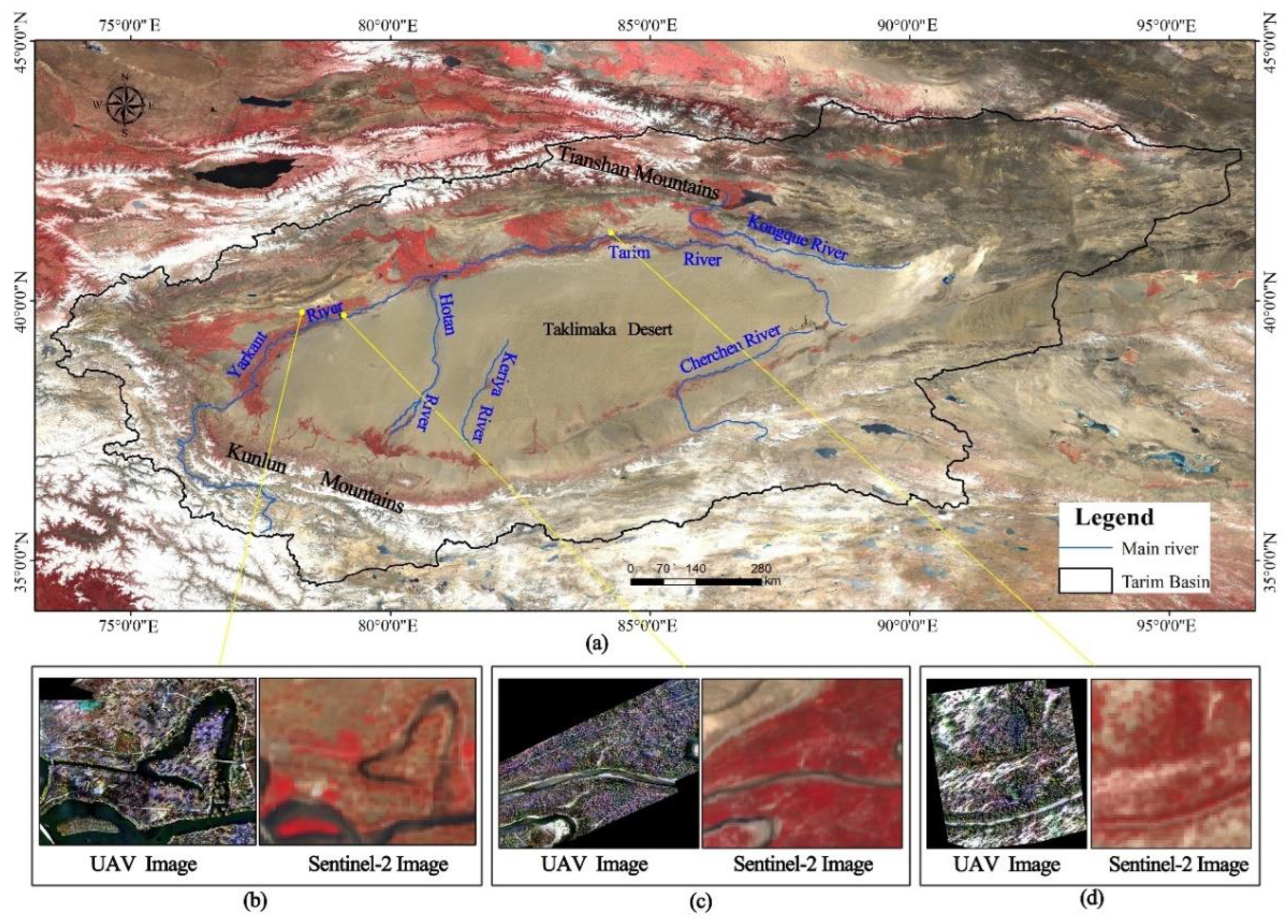
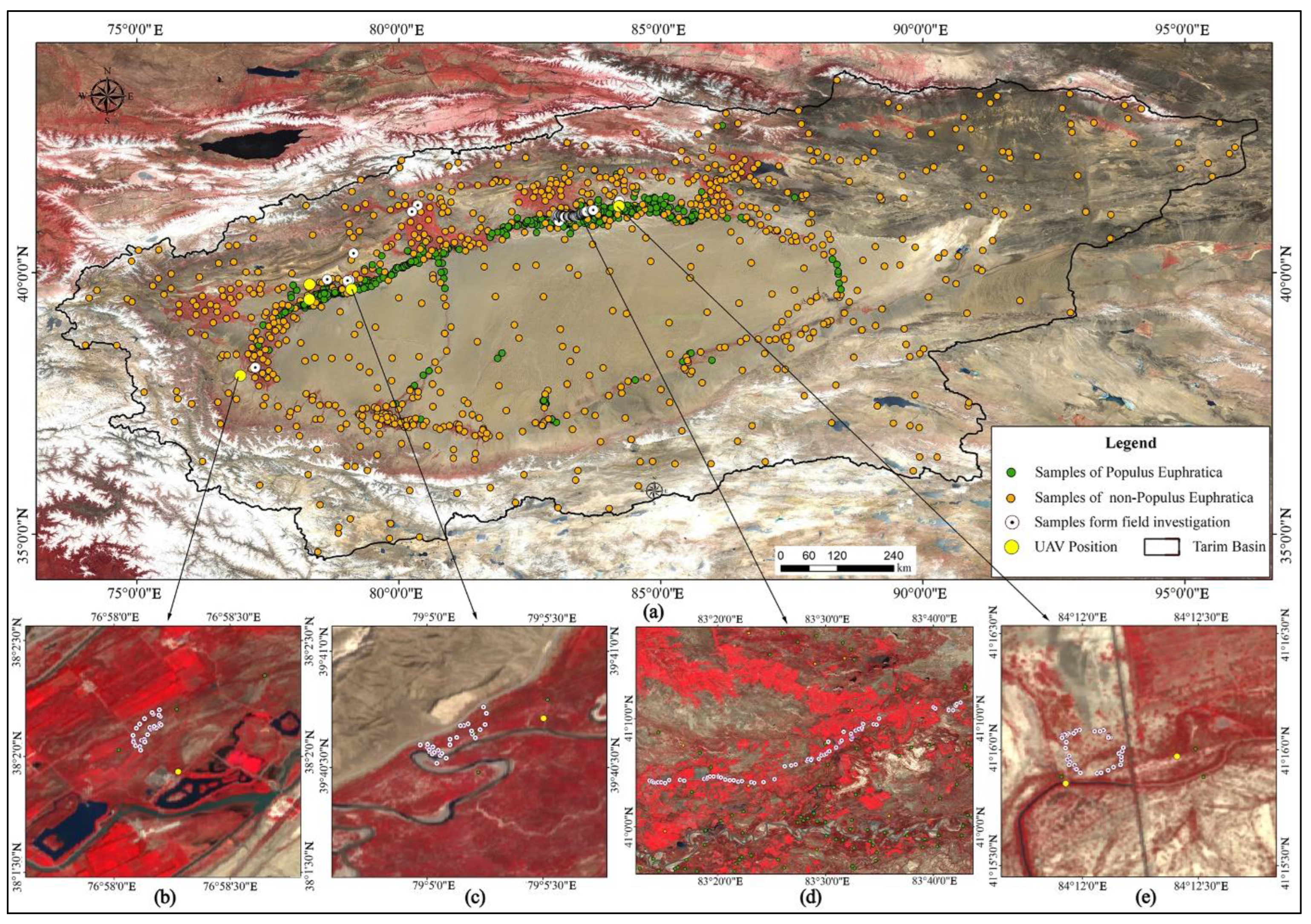
2.1. Study Area

P. euphratica is mainly distributed along riparian zones and its distributions show a corridor shape in the desert regions of western China, northern Africa, and southern Europe [23]. Approximately 61% of global P. euphratica grows in China, of which 89% grows in the Tarim River Basin (TRB) in Xinjiang [2,23]. Thus, the TRB was chosen as an example to study large-scale P. euphratica distribution mapping. The TRB is the most extensive inland basin in China, located between the Tianshan Mountains and the Kunlun Mountains in Xinjiang province (Figure 1a). It ranges from 73°24′18″E to 96°26′34″E and from 34°30′14″N to 43°54′50″N, with a total area of more than 400,000 km2. Its river system mainly consists of the Tarim River, Yarkant River, Hotan River, Kongque River, Cherchen River, and Keriya River. Its climate is a typical temperate continental climate with significant temperature differences, low rainfall, and intense evaporation [24]. The average annual air temperature is about 9–11 °C, yearly precipitation is approximately 50 mm, and the potential yearly evaporation is up to 3000 mm [25,26]. The study area’s vegetation types mainly comprise farmland, Tamarix, Alhagi, Phragmites, and forests dominated by P. euphratica [24,27].

2.2. Datasets

Table 1 briefly describes all the data used in the study, which included Sentinel-2 multispectral image (MSI), Sentinel-1 SAR image, river vector, unmanned aerial vehicle (UAV) image, and field-surveyed sample data. More detailed notes about the data selection for P. euphratica ROI detection, mapping, and validation are provided below.
(1)
ROI detection
River vector data were employed to rapidly locate the P. euphratica ROI, and they are available from the National Cryosphere Desert Data Center (http://www.ncdc.ac.cn, accessed on 18 December 2022) [28]. The TRB vector data were obtained free from the National Tibetan Plateau Scientific Data Center (https://data.tpdc.ac.cn/zh-hans/data/d5acb79d-8ffe-494e-8081-79938d2cb1fe/, accessed on 18 December 2022) [29].
(2)
P. euphratica Mapping
In this study, all the available Sentinel-2 MSI and Sentinel-1 SAR data from 2021 were used for P. euphratica mapping, and they can be freely obtained in the GEE platform. The employed Sentinel-2 MSI data included both Sentinel-2A and Sentinel-2B surface reflectance. The data have a blue band (B2: 458–523 nm), a green band (B3: 543–578 nm), a red band (B4: 650–680 nm), a near-infrared (NIR) band (B8: 785–900 nm), four red-edge bands (B5: 698–713 nm; B6: 733–748 nm; B7: 773–793 nm; B8A: 855–875 nm), and two short-wave infrared (SWIR) bands (B11: 1565–1655 nm; B12: 2100–2280 nm) [2]. The Sentinel-2 MSI data were used to extract spectral features, index features, and phenological features. Sentinel-1 dual-polarization C-band SAR provides a standard SAR strip map mode (SM), interferometric wide swath (IW), extra-wide swath (EW), and a wave mode (WV). IW is the primary acquisition mode for land observation and provides VV + VH dual polarization. The VV and VH dual polarization data from the IW mode were applied to extract backscattering features.
(3)
Validation
We went to P. euphratica-growing regions, including Shaya, Bachu, the Tarim River riparian zone, the Xiamale forest farm, and Zepu in the TRB, Xinjiang Province, from 14 October 2021 to 21 October 2021 to collect field-surveyed samples and UAV images. The field-surveyed sample data included the longitude and latitude of the location, land cover types, and vegetation types. The UAV images were obtained by launching Wu Inspire-2 UAV flights at 150 m flight heights in P. euphratica distribution regions. The UAV data had a blue band (B1: 455–485 nm), a green band (B2: 550–570 nm), a red band (B3: 658–678 nm), a red-edge band (B4: 712–722 nm), and an NIR band (B5: 820–860 nm) with a spatial resolution of 7 cm. The field-surveyed samples and the UAV data were used to validate the P. euphratica map of the study area. In addition, high-spatial-resolution images from Google Earth Map and Map World provided by the National Platform for Common Geospatial Information Service were also applied to assess the accuracy of the P. euphratica map.

3. Methodology

Progressive information extraction constrained by geoscience knowledge was adopted here. Given the geographic distribution characteristics of P. euphratica, the river vector data were first combined to rapidly locate the P. euphratica growing regions, thus avoiding unnecessary computation and improving the efficiency and precision of classification. Then, training samples were selected manually from the determined ROI. Subsequently, sensitive features, including spectra, indexes, phenology, and time-series backscattering coefficients, were designed based on all the available Sentinel-2 multispectral data and Sentinel-1 SAR data from 2021 for the ROI. Finally, the random forest (RF) model provided in GEE was used for training and to predict P. euphratica distribution with a parameter-tuning experiment. The sequence by which the real ROI was first extracted and then the P. euphratica data were extracted based on the real ROI was regarded as the progressive information extraction. Figure 2 shows the method for the large-scale mapping of P. euphratica distribution.

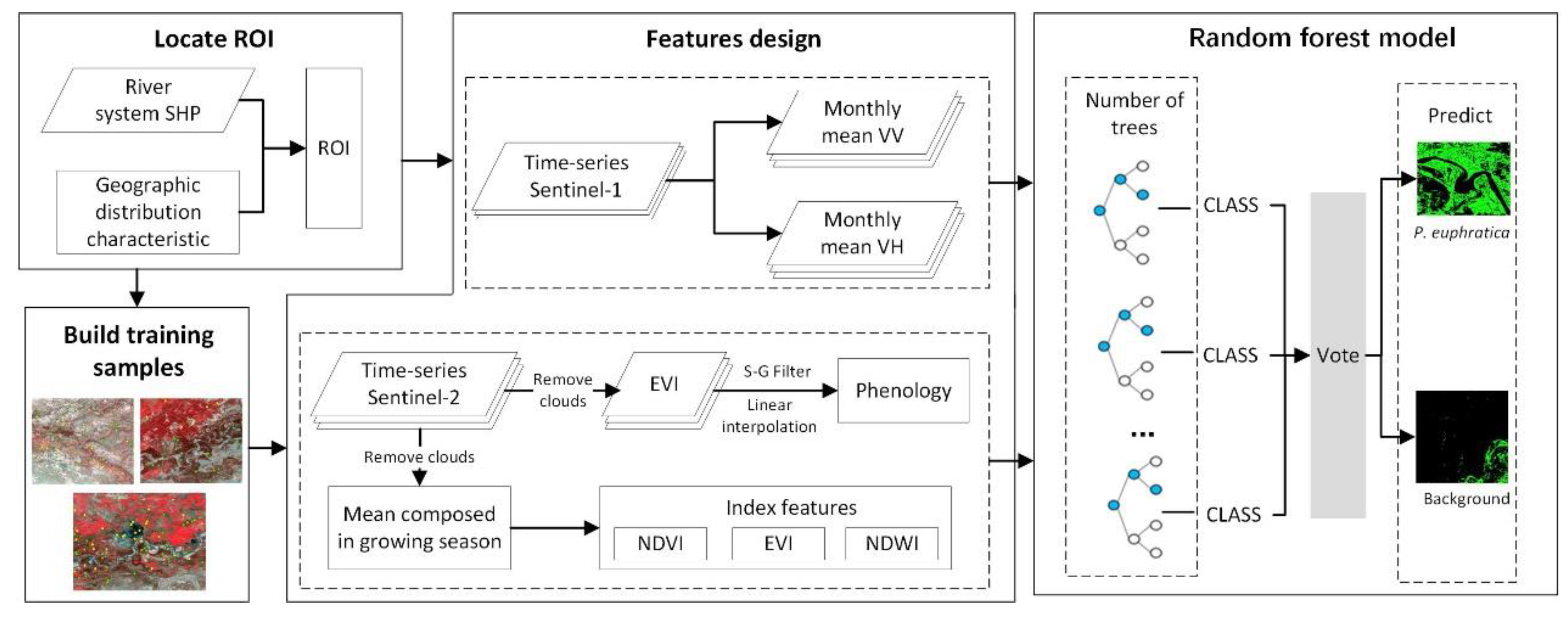
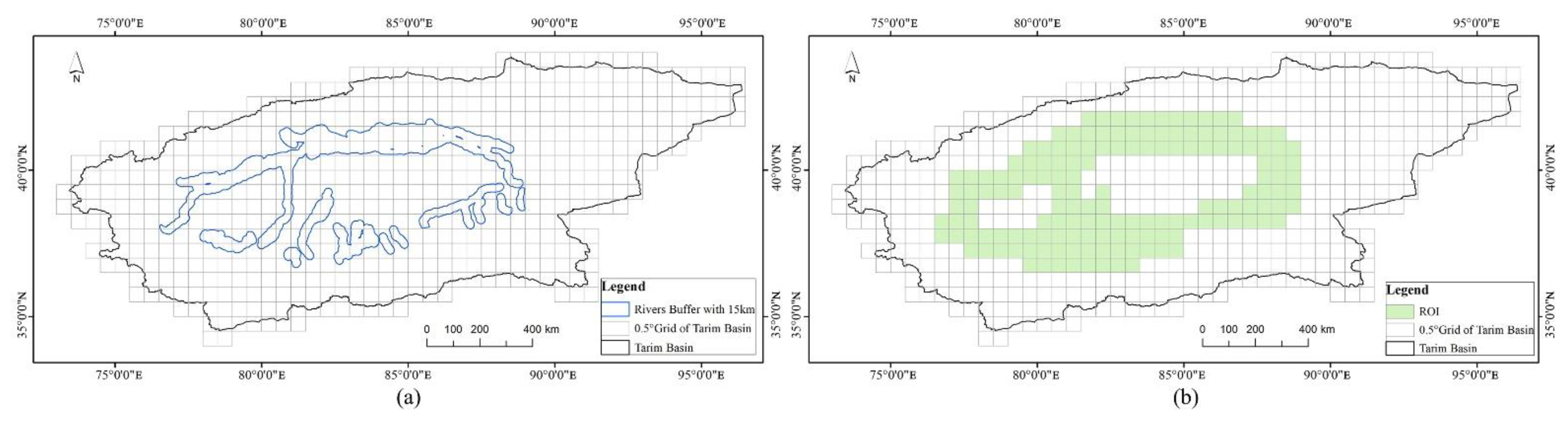
3.1. ROI Detection Based on Geographic Distribution Characteristics

As described above, P. euphratica is mainly distributed along the riparian zones in a corridor shape, so the geographic distribution characteristics were utilized to rapidly locate the real region of interest (ROI) to reduce the impact of other vegetation. Some studies have suggested that more than 80% of P. euphratica trees are distributed within 3 km of the Tarim River, and about 99% of P. euphratica trees are distributed within 10 km [2]. First, the study area was divided into a 0.5° × 0.5° grid (Figure 3a). For the river vector data located at the boundary of the grid, some P. euphratica would be missed. Therefore, a buffer zone with 15 km of the river vector was built to solve the problem. Finally, the 0.5° × 0.5° grid layer for the TRB was overlapped with the river buffer layer, and the grids containing the river buffer were considered as the real ROI for P. euphratica (the green region in Figure 3b). The area of the real ROI was a quarter of the original study area. ROI detection based on geographical distribution characteristics can reduce computing time and the number of other objects easily confused with P. euphratica and significantly improve the efficiency and accuracy of large-scale P. euphratica mapping.

3.2. Land Surface Phenology Estimation

All the available Sentinel-2 EVI data for 2021 were used to estimate the land surface phenology. However, there was some noise in the time-series EVI due to the influence of clouds and rain, so it was necessary to reconstruct the time-series EVI before estimating the land surface phenology.

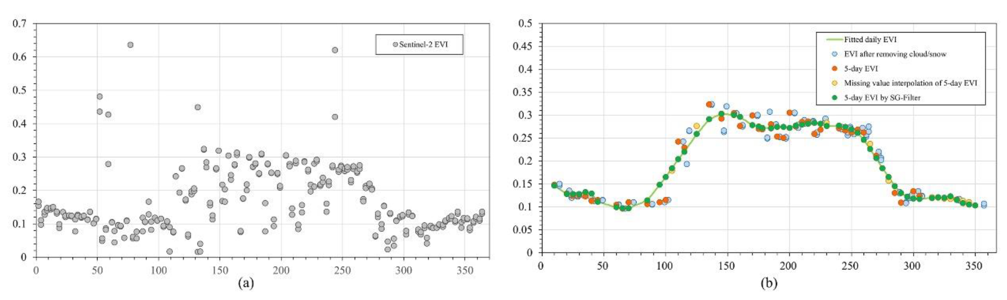
3.2.1. Time-Series EVI Reconstruction Based on S-G Filter

The annual time-series EVI was calculated using Equation (1) [30] after removing the cloud-based noise from all the available Sentinel-2 MSI data for 2021.
E V I = G ( ρ n ρ r ) ( ρ n + C 1 ρ r C 2 ρ b + L )
where ρ b , ρ n , and ρ r are the surface reflectance of the Sentinel-2 blue band (B2), red band (B4), and NIR band (B8); G   = 2.5; C 1   = 6; and C 2 = 7.5 .
The Savitzky–Golay (S-G) filtering method was proposed first by Savitzky and Golay for the smoothing of time-series data and it is based on a least-squares convolution method [14,22,31]. It has been widely applied to reconstruct time-series remote sensing data and is regarded as a practical denoising method for time-series remote sensing images [14,32]. The S-G filter uses a sliding window size to convolve with the time-series data. Then, the minimum root-mean-square error (RMSE) was obtained by performing a weighted polynomial fitting. Equation (2) shows the calculation expression [31].
E V I k , f i t = 1 2 m + 1 i = m i = m C i E V I k + i
where E V I k ,   f i t is the fitted EVI with the S-G filter,   E V I k + i is the original EVI, m is the size of half a sliding window, 2   m + 1 is the size of a sliding window, and C i is the filtering coefficient calculated with a polynomial. The size of the sliding window was 2   m + 1 . Every EVI in the window could be then expressed as E V I = ( m , m + 1 , , 1 ,   0 ,   1 , , m 1 ,   m ) . If the n 1 degree polynomial is used to fit the EVI in the window, there will be 2   m + 1  n-element linear equations (Equation (3)). Furthermore, when 2 m + 1 n , C i can be determined with the least-squares method [32]. Therefore, the size of the sliding window ( m ) and the number of terms for the smooth polynomial ( n ) should be determined first, which usually depends on specific situations. In this work, n = 3 and m = 7 .
E V I f i t = c 0 + c 1 E V I + c 2 E V I 2 + + c n 1 E V I n 1
The first m and last m data of the time-series EVI cannot be fitted, although they participated in the fitting for the S-G filter. To solve this problem, we extended the annual time-series data for 2021 to include the longer time series from 1 October 2020 to 1 April 2022. In addition, the time-series EVI cannot be fitted with the S-G filter when missing values exist. Therefore, a linear interpolation method was adopted to process missing values before denoising. The detailed steps for the time-series EVI reconstruction are described below:
(1)
Time-series Sentinel-2 MSI data from 1 October 2020 to 1 April 2022 were reprocessed by removing clouds or cloud shadows and then the time-series EVI was calculated with Equation (1). Figure 4a displays the time-series EVI without the removal of clouds or cloud shadows, and the blue points in Figure 4b show the time-series EVI with the removal of clouds and cloud shadows. It can be seen that removing clouds and cloud shadows made it possible to remove most of the noise but could cause some missing values;
(2)
A moving average window of 5 days was then applied to generate a 5 day mean composited time-series EVI to reduce the computational cost of the following S-G filtering. Orange points in Figure 4b display the 5 day mean composite time-series EVI;
(3)
The linear interpolation method was used to estimate the missing values for the 5 day mean composite time-series EVI to avoid an underdetermined equation occurring in the S-G filtering. The yellow points in Figure 4b show where the missing values in the 5 day EVI were interpolated;
(4)
The S-G filter was adopted to smooth the interpolated 5 day time-series EVI, and the smooth and continuous time-series EVI was then fitted. Green points in Figure 4b show the 5 day EVI obtained after S-G filtering;
(5)
The daily EVI was finally fitted using the linear interpolation method. The green line in Figure 4b indicates the daily EVI.

3.2.2. Phenology Extraction

The land surface phenology, including the start of season time (SoS), end of season time (EoS), length of the season (LoS), maximum value of annual time-series EVI data (MaxV), date of maximum value (DoM), and amplitude of season (AoS), was subsequently extracted based on the daily EVI in 2021. The SoS is the date when the EVI time series showed a continuous upward trend, and the EoS is the date when the EVI time series showed a continuous downward trend. This study used a threshold method [16,19] to estimate the SoS and EoS. Generally, the date when the EVI increased to 50% of the annual time-series amplitude was regarded as the SoS, and the date when the EVI decreased to 50% of the annual time-series amplitude was regarded as the EoS [19]. The EVI at the SoS or EoS was expressed as the threshold μ, and μ was calculated with Equation (4). The LoS is the length of the period from the SoS to the EoS; that is, L o S = E o S S o S . The AoS is the difference between the maximum EVI and the base EVI (BoS). The BoS was expressed as the average of the minimum EVI on the left of the SoS and on the right of the EoS in this study. The MaxV is the maximum EVI for the annual time-series data and represents the vegetation greenness. The DoM is the date when the EVI reached the maximum.
μ = E V I m a x E V I m i n 50 % + E V I m i n
where E V I m a x and E V I m i n are the maximum EVI and the minimum EVI for the annual time-series data in 2021, respectively.

3.3. P. euphratica Distribution Mapping via GEE

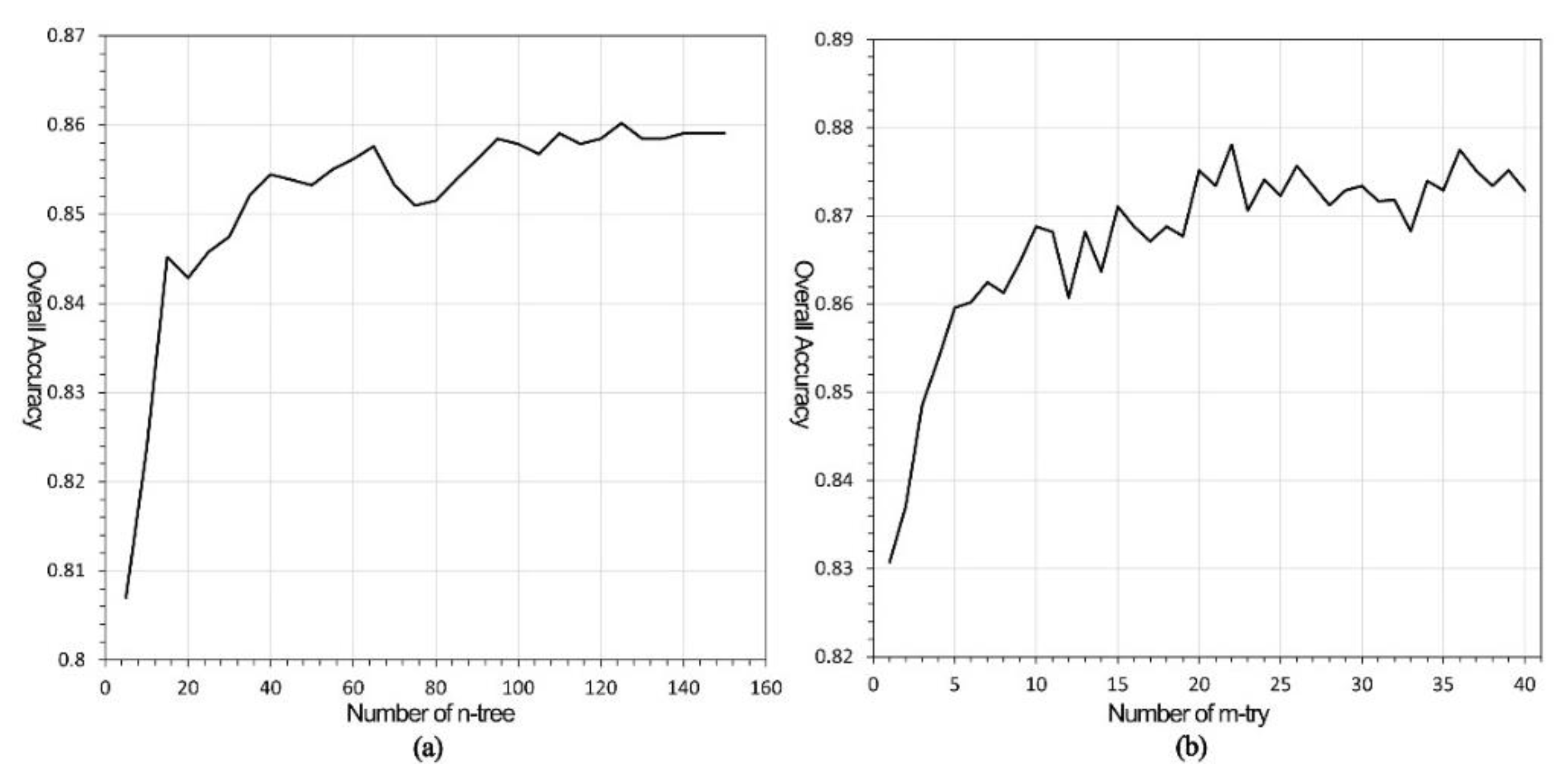
3.3.1. Random Forest Model

Sensitive features for P. euphratica were designed as feature inputs for the RF model based on time-series Sentinel-2 MSI data and time-series Sentinel-1 SAR data in the GEE platform. The RF algorithm provided by GEE was then used for model training based on training samples to generate the classification model, and the P. euphratica distribution result was finally produced. The key factors that determine the accuracy of a random forest classifier include input features, training samples, the number of decision trees (n-tree), and the number of features used for the binary tree of a node (m-try). In theory, the greater the number of decision trees and features used for a node, the more complicated the RF model is and the higher the RF classifier’s accuracy. Nevertheless, this also leads to higher costs in terms of calculation time [33]. Different numbers for n-tree and m-try were debugged to find the best parameters. Figure 5 illustrates the debugging results for the two parameters. Figure 5a shows that the overall accuracy was the highest when the number of decision trees was 125, while Figure 5b shows that the overall accuracy was the highest when the number of features used for the binary tree of a node was 22. Therefore, the numbers for n-tree and m-try were set to 125 and 22, respectively, in this study.

3.3.2. Training Data

The characteristics of the P. euphratica forests appearing in the remote sensing images were first analyzed by connecting the field investigation samples and the UAV aerial images of the P. euphratica forests with Sentinel-2 MSI images. Figure 1b–d demonstrate the performances for sparse P. euphratica forest, dense forest, and sparse–dense forest, respectively, with the Sentinel-2 MSI and UAV images. To make the vegetation types that could be easily confused with P. euphratica clearer, some training data were first generated randomly to predict a preliminary result. Figure 6 shows some objects easily misclassified as P. euphratica forests. It was found that allée trees, urban green land, vegetation in wetlands, and some farmlands could be easily misclassified as P. euphratica forests by visual comparison. Therefore, when selecting negative samples, it was necessary to focus on allée trees, urban green land, vegetation in wetlands, and farmland. Only pure pixels of P. euphratica were selected to avoid pixels near the boundaries of the P. euphratica forests. A total of 5755 samples were collected for this study, including 2438 positive and 3317 negative samples.

3.3.3. Sensitive Features for P. euphratica

Spectral features, indices, phenological features, and backscattering features were designed as sensitive features for P. euphratica in this study. The spectral features included the surface reflectance of the blue band (B2), green band (B3), red band (B4), NIR band (B8), and four red-edge bands (B5, B6, B7, B8A) from the Sentinel-2 MSI data. Some indices calculated with Sentinel-2 spectral bands were also used in this study to enhance the information for classification, including the NDVI [19], EVI, and normalized difference water index (NDWI) [34]. The widely used vegetation indexes NDVI and EVI were chosen for this study. However, since P. euphratica trees grow along riverbanks and some grow in shallow water in rivers or lakes, the NDWI was also used as an input feature. As Section 3.2 described, the SoS, EoS, LoS, DoM, and AoS were designed as phenological features. As phenology extraction involves annual time-series EVI S-G filtering and linear interpolation with a 10 m spatial resolution, the amount of data and computation required were tremendous at a large scale. The estimated phenological features were first exported to ASSETS (a cloud disk assigned to a user) in the GEE platform to avoid problems; e.g., running out of memory or calculation over time. All the available VV and VH for the Sentinel-1 SAR data for each month were averaged as the monthly VV and VH data in 2021. The monthly VV and VH were designed as backscattering features in this study.

3.4. Assessment

The field-surveyed samples and randomly generated samples were regarded as validation samples for the assessment of the precision of the proposed method in the work. Figure 7 displays the distribution of randomly generated samples, field-surveyed samples, and UAV data. A stratified random sampling method was used to generate validation samples automatically. Adding 302 field-surveyed samples, a total of 1535 validation sample data were finally generated, including 702 P. euphratica samples and 833 negative samples. UAV data and high-spatial-resolution data from Google Earth Map and Map World were also employed as reference data to quantitatively assess the precision of the results using the commission error (CE), omission error (OE), and overall accuracy (OA) [33]. It was assumed that the number of samples correctly identified as P. euphratica was N 11 , that the number of samples correctly classified as non-Populus euphratica was N 22 , that the number of real P. euphratica samples misclassified as others was N 21 , and that the number of samples wrongly predicted as P. euphratica was N 12 . The expressions for the CE, OE, and OA rates for P. euphratica are described below.
Commission error (CE): N 12 / ( N 11 + N 12 ) , the ratio of wrongly predicted P. euphratica samples to the total number of samples classified as P. euphratica in the results [33];
Omission error (OE): N 21 / ( N 11 + N 21 ) , the ratio of real but undetected P. euphratica samples to the total number of authentic P. euphratica samples [33];
Overall accuracy (OA): ( N 11 + N 22 ) / ( N 11 + N 21 + N 12 + N 22 ) , the ratio of correctly classified samples to the total number of samples [33].

4. Results and Analysis

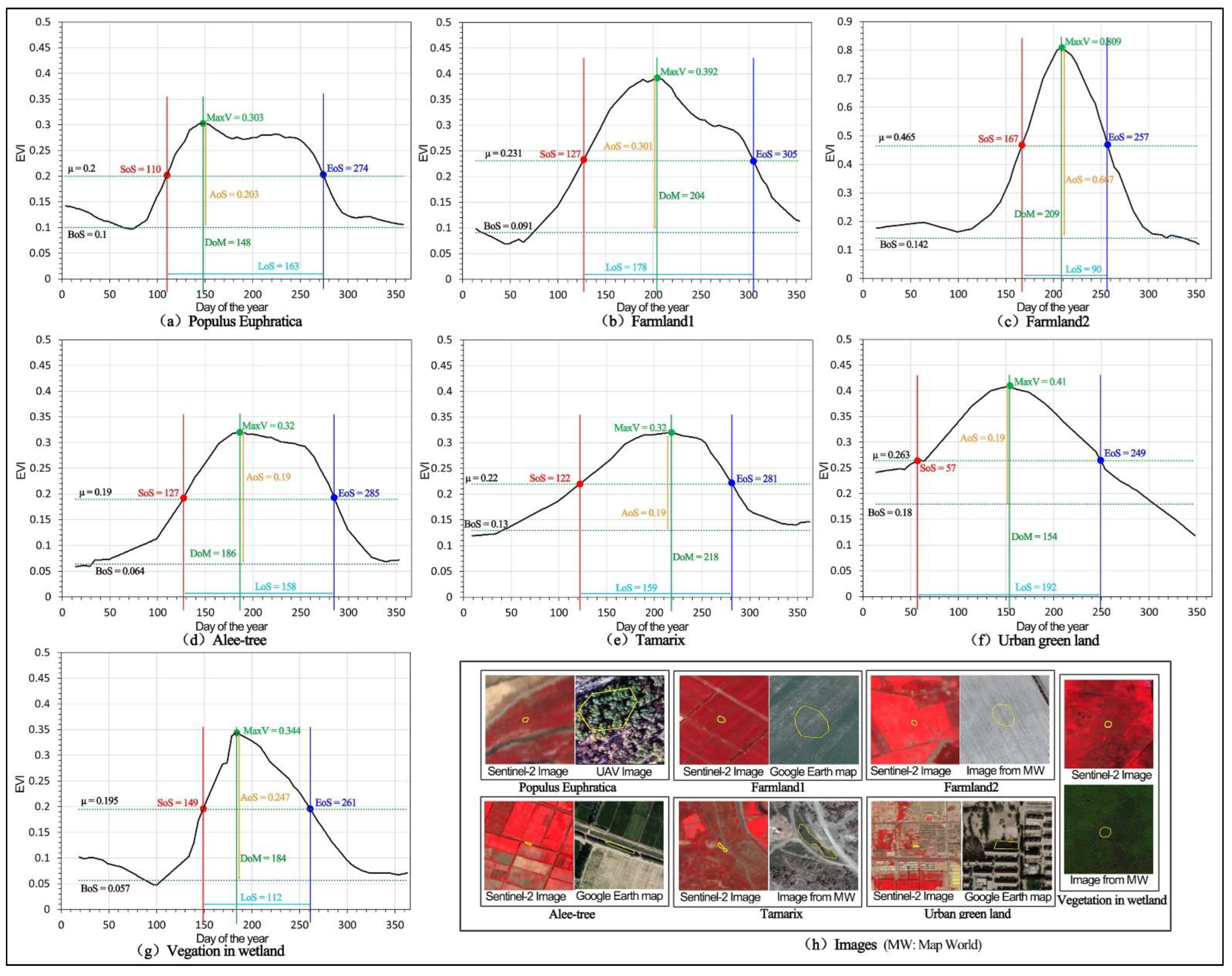
4.1. P. euphratica Phenology Analysis

Figure 8h displays Sentinel-2 and UAV images, as well as high-spatial-resolution images from Google Earth Map and Map World, of P. euphratica, two kinds of farmland, allée trees, Tamarix, urban green land, and vegetation in wetlands. It shows that the appearance of P. euphratica in the Sentinel-2 images was very similar to that of the other kinds of vegetation, except for cotton land (farmland 2). It was difficult to correctly identify P. euphratica using only spectral and index features. The mean values of the selected regions (shown as yellow polygons in Figure 8h) were used to show the EVI phenological curves of the different vegetation types in 2021, as illustrated in Figure 8a–g. It can be seen that the SoS of P. euphratica was 20 April, the EoS was 1 October, the LoS was 163 days, the DoM was 28 May, and the AoS was 0.203. Li et al. determined that the SoS was in late April and the EoS was in October when using time-series Global Land Surface Satellite (GLASS) LAI to analyze the phenology of P. euphratica in the upper reaches of Tarim River [32]. Our results are well in line with the results of Li’s team. The DoM for P. euphratica was much earlier than that for other vegetation types, except for urban green land; for example, it was nearly two months earlier than those for farmland and Tamarix and more than one month earlier than those for allée trees and vegetation in wetlands. The DoM for P. euphratica was only 6 days earlier than that for urban green land, but its SoS and EoS were approximately 40 days and 25 days later than those for urban green land. The EoS for P. euphratica was nearly a half a month earlier than for other vegetation types, except for urban green land, and it was 50 days later than for urban green land. The results indicated that phenological characteristics could be used to distinguish P. euphratica from other types of vegetation with which it is easily confused.

4.2. Performance Analysis of Specific Features

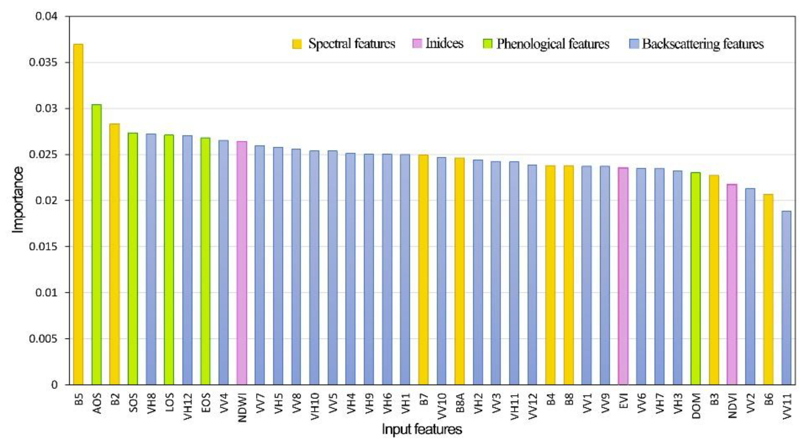
4.2.1. Importance Analysis of Features

RF models can show the importance of input features by assigning a score, so the importance of the input features for classification was used to compare their performance. To make the importance scores of these features easier to understand, they were first normalized, and the sum of the normalized data was limited to 1. Figure 9 shows the normalized importance of the input features for the RF model. The differences between the scores for these 40 features were small, and the scores for 37 features were within the range [0.02, 0.03]. This indicated that all the used features were important for classification.
A total of 40 input features were used in the model, and the average importance score was 0.025. Therefore, features with importance scores greater than 0.025 were considered more important for the classification of the model than the others. There were 18 features with scores greater than 0.025, including 2 spectral features (Sentinel-2 band 5 and band 2), the NDWI, 4 phenological features (AoS, SoS, EoS, and LoS), and 11 SAR backscattering features (Sentinel-1 monthly mean VV data for April, May, July, and August 2021 and monthly mean VH data for April, May, June, July, August, September, October, and December 2021). Among these features, the two spectral and four phenological features had relatively higher scores than the backscattering features, and all of them were ranked in the top ten. The results suggested that the spectral and phenological features exerted a significant influence on the extraction of the distribution of P. euphratica forests and that incorporating indices and backscattering features could further enhance the classification precision of the RF model. When classifying P. euphratica, the Sentinel-2 red-edge band (band 5) and blue band among the spectral features, the NDWI among the indices features, the phenological features, and the VH polarized backscattering features for the Sentinel-1 SAR satellite data—particularly the VH polarized data obtained during August and December—exhibited higher degrees of sensitivity in recognizing P. euphratica.

4.2.2. Comparison Analysis
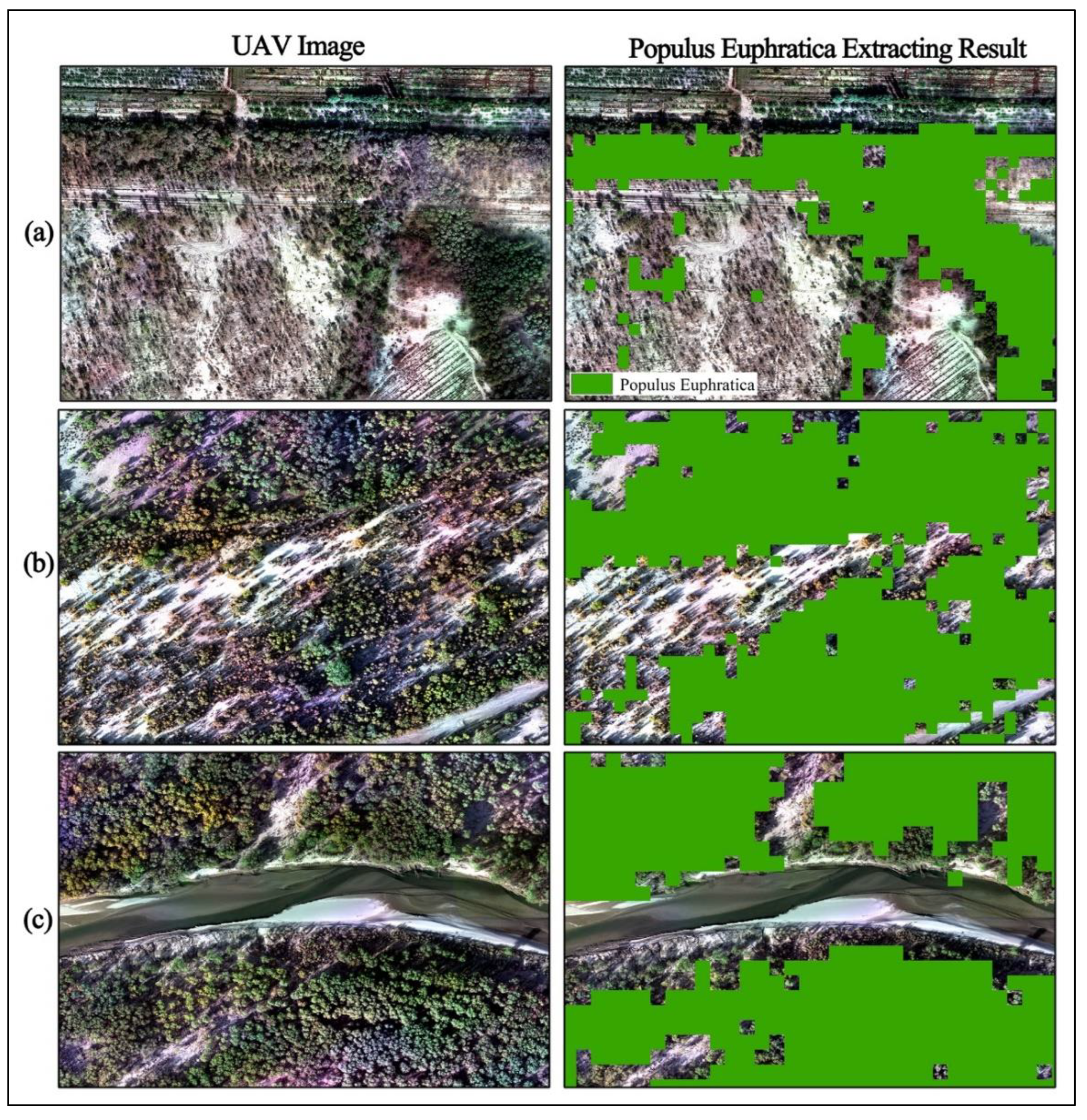
In order to explain the performance of the phenological features and backscattering features in large-scale P. euphratica mapping, three experiments were carried out with three different sets of input features, holding the other parameters the same. Table 2 listed briefly input features for the three experiments. The input features of experiment one were only the spectral features and indices, which were described in Section 3.3.3 in detail. Experiment two added phenological features to the spectral features and indices. Experiment three employed the method proposed in this paper, and it added phenological features and backscattering features to the spectral features and indices. The results of the three experiments were then compared visually.
Figure 10 shows the P. euphratica distributions obtained in experiment one, experiment two, and experiment three in the study area. It demonstrates that the P. euphratica distribution in experiment one was more extensive than that in experiment two, and that in experiment two was also more extensive than that in experiment three; these distributions were mainly located in the regions shown as yellow rectangles in Figure 10a. It can be seen that the land cover in these regions is mainly farmland, urban land, and wetlands, with fewer P. euphratica trees. The extra P. euphratica distributions obtained in experiments 1 and 2 were not real P. euphratica. The visual comparison suggested that only the addition of phenological features could solve the issues concerning other vegetation being misclassified as P. euphratica, at least to a certain degree, but the addition of phenological features and backscattering features significantly contributed to better identification of P. euphratica trees and the ability to distinguish them from these other types of vegetation.
The detailed maps for the three experiments were visually compared to further analyze the performance of the phenological and backscattering features. Figure 11 displays the detailed maps for experiment one, experiment two, and experiment three for regions without P. euphratica distribution. Experiment one misclassified some urban green land (Figure 11a), vegetation in wetlands (Figure 11b), and farmland and allée trees (Figure 11c) as P. euphratica. Experiment two, with only phenological features added, dramatically reduced misclassification for some urban green land, farmland, and Allée trees, as Figure 11a,c show, and it slightly reduced misclassification for some vegetation in wetlands, as Figure 11b shows. Experiment three, however, with backscattering features also added, further reduced misclassification compared to experiment two, especially for vegetation in wetlands. Moreover, experiment three, with the addition of phenological features and backscattering features, significantly improved identification of P. euphratica and reduced misclassification of these other types of vegetation in comparison to the results for experiment one. The compared results indicated that phenological features performed well in distinguishing P. euphratica from some urban green land, farmland, and allée trees, but the backscattering features performed better than the phenological features in distinguishing P. euphratica from some vegetation in wetlands. Therefore, adding phenological and backscattering features can effectively reduce misclassification errors involving P. euphratica and other vegetation.
Figure 12 shows detailed maps of the experiment one, experiment two, and experiment three in areas that were presented as mainly consisting of P. euphratica. Figure 12a shows a visual comparison of generally dense P. euphratica forests. It demonstrates that dense P. euphratica forests were correctly predicted in these three results. However, some sparse P. euphratica forests were not detected in experiment one but were detected in experiments 2 and 3 (as the purple ellipse shows in Figure 12a). As the yellow ellipses show in Figure 12a, some farmland and grassland were misclassified as P. euphratica in the results from experiment one, while only a minority of these types of vegetation were misclassified as P. euphratica in the results from experiment two, and they were all correctly identified in the results from experiment three. Figure 12b displays a visual comparison of P. euphratica and farmland. There are large areas of farmlands in Figure 12b. Some farmland areas were misclassified as P. euphratica in experiment one, and a few were misclassified as P. euphratica in experiment two, but they were correctly predicted in experiment three (as shown by the yellow ellipses in Figure 12b). Figure 12c shows a visual comparison of sparse P. euphratica forests. The comparison results revealed that only adding phenological features made it possible to detect P. euphratica in sparse forests, as did adding phenological features and backscattering features, but that adding phenological features and backscattering features made it possible to distinguish P. euphratica from farmland more effectively than only adding phenological features.
The results of the visual comparison revealed that the method used in experiment three could not only correctly distinguish P. euphratica from other types of vegetation but could also detect P. euphratica well in sparse forests. In conclusion, the method proposed in this paper with phenological and backscattering features as input for the RF model performed much better than the method with only spectral features and index features.

4.3. Validation

Table 3 shows the confusion matrix for the precision validation of experiment one, experiment two, and experiment three. It was generated by referencing the field-surveyed samples, UAV images, and high-spatial-resolution images from Google Earth Map and Map World. The CE, OE, and OA rates for experiment one, experiment two, and experiment three were finally calculated from the confusion matrix (Table 3), as listed in Table 4. The method using only spectral data and indices misclassified some farmland, allée trees, urban green land, and vegetation in wetlands as P. euphratica, and its OE and CE reached higher than 21% and 28%, respectively, while its OA was only 76%. The OE, CE, and OA rates for the method with the addition of phenological features were 13.25%, 19.34%, and 84.43%, respectively, which were increases of approximately 8%, 9%, and 8% in comparison to the results for experiment one. The OE, CE, and OA rates for the method proposed in this paper were 12.53%, 11.01%, and 89.32%, respectively, which were increases of approximately 1%, 8%, and 5% in comparison to the results for experiment two and of approximately 9%, 17%, and 13% in comparison to the results for experiment one. The results indicated that only adding phenological features could reduce not only omission errors but also commission errors, while adding backscattering features could further improve the classification accuracy for commission. Therefore, the phenological and backscattering features adopted in the proposed method had good effects on P. euphratica classification at a large scale, and they significantly improved the accuracy for large-scale P. euphratica distribution mapping.

5. Discussion

The results of the analysis of the features indicated that all the spectral features, indices, phenological features, and backscattering features used played important roles in the classification of P. euphratica. The spectral features and phenological features had significant influences on the extraction of P. euphratica forests, and incorporating indices and backscattering features further enhanced the classification precision. Sentinel-2 band 5 and band 2 were the spectral features most sensitive to P. euphratica. Previous studies have found that Sentinel-2 band 5 responds best among the red-edge bands for vegetation observation [11,35]. Regarding spectral indices, the NDWI was more sensitive than the NDVI and EVI in extracting P. euphratica. The main reason was that P. euphratica trees mainly grow along riverbanks, and some even grow in water. The NDVI and EVI are often the preferred indices for vegetation classification. However, perhaps due to the incorporation of various vegetation-related features in this study, such as red-edge bands and phenological characteristics, the importance of the NDVI and EVI was relatively lower compared to the NDWI. The selected phenological features, including the SoS, EoS, LoS, and AoS, were highly sensitive in the extraction of P. euphratica. Compared with the results obtained when only using spectral data and indices, the OE, CE, and OA rates obtained with the method involving only the addition of phenological features were improved by approximately 8%, 9%, and 8%, respectively. This indicated that the accuracy of P. euphratica classification in terms of omission and commission errors could be improved by about 8% after adding phenological features. It was found that the phenological characteristics for the different types of vegetation were unique, as discussed in Section 4.1. Therefore, the inclusion of phenological features can improve the classification accuracy for vegetation to a certain extent. Some other studies have also pointed out that phenological features can effectively improve the accuracy of vegetation classification [36,37]. In terms of backscattering features, Sentinel-1 SAR VH polarization data were more sensitive than VV polarization data for P. euphratica extraction. With the addition of backscattering features and phenological features, the OE, CE, and OA rates for P. euphratica extraction were improved by about 1%, 8%, and 5%, respectively. It can be concluded that backscattering features improved the overall accuracy by approximately 5%, especially for P. euphratica commission, while they had no significant effect on P. euphratica omissions. Blaes et al. revealed that optical remote sensing data make the dominant contribution to mapping accuracy, and SAR data can be used to further enhance mapping accuracy by over 5% by comparing optical images with SAR data [17]. Therefore, it can be inferred that the precision of distribution mapping of P. euphratica in large areas can be substantially enhanced by incorporating phenological and backscatter features, as introduced in this study.
The comparison and validation results suggested that the proposed method could significantly improve the accuracy of P. euphratica classification in terms of omission and, especially, commission. The improvement in the OE rate was much lower than for the CE rate, which was mainly caused by the scale effect with remote sensing images. Figure 13 shows the mapping results for P. euphratica forests with different densities; on the left is the UAV image, and on the right is the result with 10 m spatial resolution. The P. euphratica trees in the Sentinel-2 image of the dense forest were ideally classified (Figure 13b,c), but the P. euphratica trees in the Sentinel-2 image of the very sparse forest were not detected (Figure 13a,b). The reason for this was that the crowns of P. euphratica trees are so tiny that they present very mixed pixels in remote sensing data with 10 m spatial resolution when P. euphratica is distributed very sparsely. Combining higher-spatial-resolution remote sensing data, such as that from SPOT-5/6 or Gaofen-1/2, can improve sparse P. euphratica detection. The geographical distribution characteristics of P. euphratica, phenological features, and backscattering features were utilized to greatly reduce the interference from other vegetation types, but a few regions were still misclassified as P. euphratica. Most of the isolated misclassified pixels could be treated as noise resulting from the pixel-based classification method and could be removed through the post-classification process.
Although the proposed method was studied by taking the TRB as an example, it could be applied to map P. euphratica distributions in larger regions based on subzones, such as at the national or global scales, due to the discontinuities of P. euphratica distributions. It can adapt the phenological differences for different regions and ensure the accuracy of P. euphratica distribution mapping in larger regions. To prove the feasibility of our proposed method for subzone concepts, we plan to conduct mapping experiments involving P. euphratica distributions at the national or global scales in the future.

6. Conclusions

Due to the difficulties of large-scale P. euphratica distribution mapping, a new method was proposed in this paper. The geographical distribution characteristics of P. euphratica were first utilized to rapidly locate the real ROI, and then spectral features, indices, phenological features, and backscattering features derived from all the available Sentinel-2 MSI and Sentinel-1 SAR data for 2021 were used as the input for an RF model to classify P. euphratica in the GEE platform. The results were finally compared through visual and quantitative evaluation with the results for the method using only spectral features and indices and for that only using phenological features.
(1)
The geographical distribution characteristics of P. euphratica growing along riverbanks in a corridor shape were used to rapidly locate the real ROI based on river vector data. Then, the complexity of the background and interference from similar objects could be significantly reduced;
(2)
The spectral features and phenological features made dominant contributions to the accurate extraction of P. euphratica, and adding indices and backscattering features could further enhance the classification precision. Phenological features could enhance the accuracy of P. euphratica classification in terms of omission and commission errors by about 8%. Adding backscattering features made it possible to further improve the accuracy of P. euphratica commission by approximately 8% while having little effect on P. euphratica omissions;
(3)
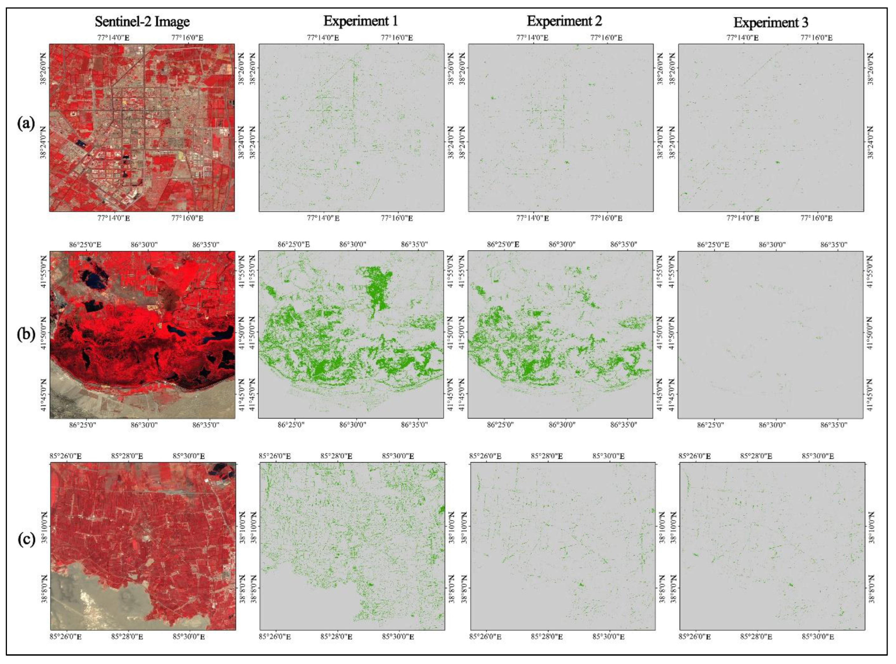
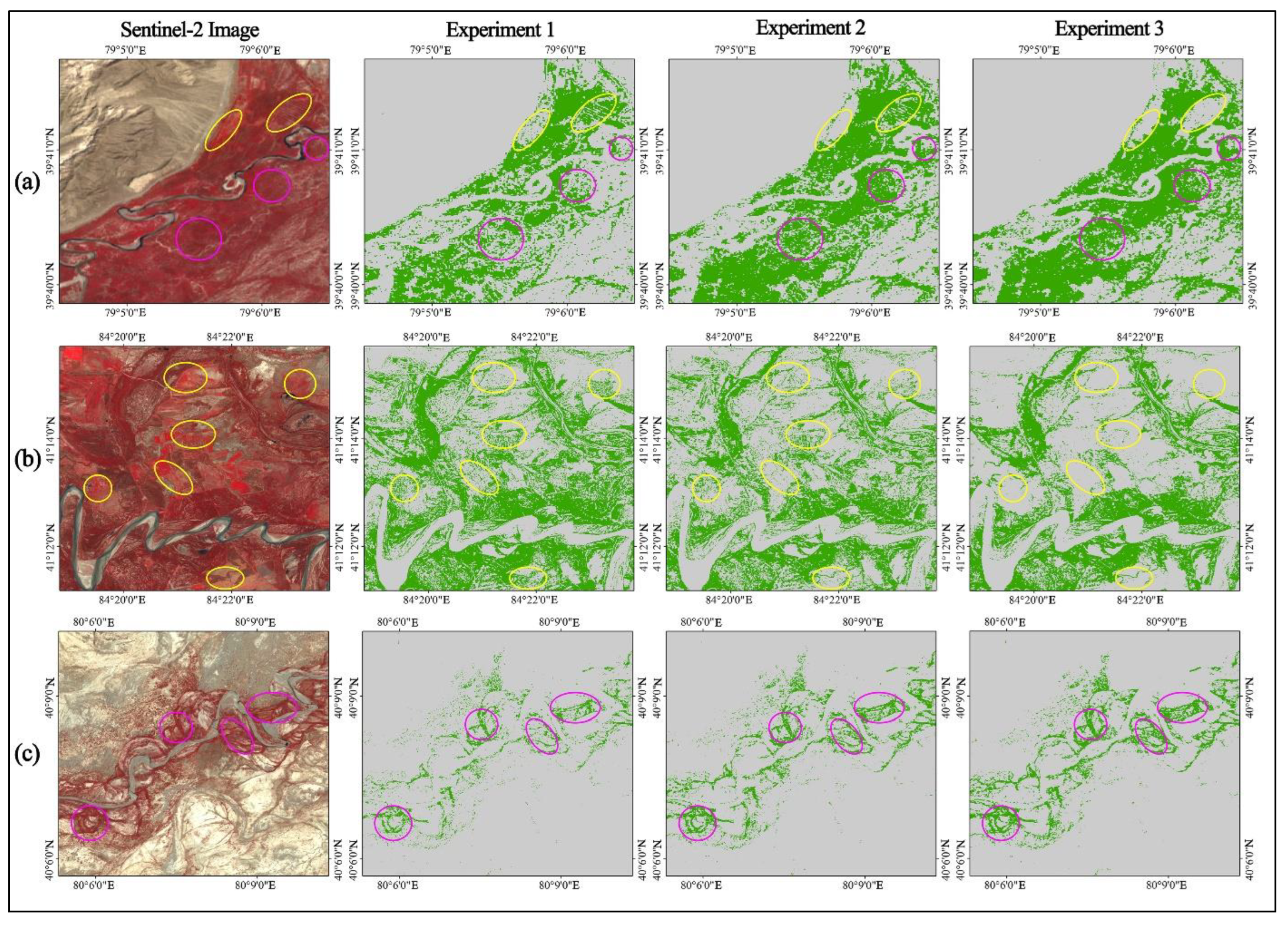
The method of adding phenological and time-series backscattering features made it possible to correctly distinguish P. euphratica from other vegetation types that have similar spectral features to P. euphratica; e.g., some farmland areas, urban green land, Tamarix, allée trees, and vegetation in wetlands;
(4)
The proposed method’s OE, CE, and OA rates were 12.53%, 11.01%, and 89.32%, respectively, which represented increases of approximately 9%, 17%, and 13% in comparison to the method using only spectral features and indices. It greatly improved the accuracy of P. euphratica classification in terms of both omission and, especially, commission. The increased OE rate was much lower than the CE rate, which was mainly due to the scale effect associated with remote sensing images.

Author Contributions

Conceptualization, G.H. and G.W.; methodology, Y.P.; software, Y.P.; validation, Y.P. and G.W.; formal analysis, Y.P. and Z.Z; investigation, Y.P. and Z.Z; resources, Y.P.; data curation, Y.P.; writing—original draft preparation, Y.P.; writing—review and editing, G.H.; visualization, Y.P.; supervision, G.W. and Z.Z.; project administration, G.H.; funding acquisition, G.H. All authors have read and agreed to the published version of the manuscript.

Funding

This research was funded by the Strategic Priority Research Program of the Chinese Academy of Sciences under grant number XDA19090300, the Second Tibetan Plateau Scientific Expedition and Research Program (STEP, grant no. 2019QZKK0307), and the National Natural Science Foundation of China (NSFC, grant no. 62101531).

Data Availability Statement

The Sentinel-1/2 data used in this research were available in the GEE platform (https://code.earthengine.google.com/, accessed on 1 March 2023). The river vector data were downloaded from the National Cryosphere Desert Data Center (http://www.ncdc.ac.cn, accessed on 18 December 2022). The Tarim River Basin vector data were obtained free from the National Tibetan Plateau Scientific Data Center (https://data.tpdc.ac.cn/zh-hans/data/d5acb79d-8ffe-494e-8081-79938d2cb1fe/, accessed on 18 December 2022).

Conflicts of Interest

The authors declare no conflict of interest.

References

  1. Thomas, F.M.; Jeschke, M.; Zhang, X.; Lang, P. Stand structure and productivity of Populus euphratica along a gradient of groundwater distances at the Tarim River (NW China). J. Plant Ecol. 2017, 10, 753–764. [Google Scholar] [CrossRef] [Green Version]
  2. Peng, Y.; He, G.J.; Wang, G.Z. Spatial-temporal analysis of the changes in Populus euphratica distribution in the Tarim National Nature Reserve over the past 60 years. Int. J. Appl. Earth Obs. Geoinf. 2022, 113, 103000. [Google Scholar] [CrossRef]
  3. Deng, X.Y.; Xu, H.L.; Yang, Z.F. Distribution characters and ecological water requirements of natural vegetation in the upper and middle reaches of Tarim River, Northwestern China. J. Food Agric. Environ. 2013, 11, 1156–1163. [Google Scholar]
  4. Eziz, M.; Yimit, H.; Halmurat, G.; Amrulla, G. The landscape patterns change of Tarim Populus Nature Reserve and its ecoenvironmental effects, Xinjiang, China. In Proceedings of the SPIE 7145, Geoinformatics 2008 and Joint Conference on GIS and Built Environment: Monitoring and Assessment of Natural Resources and Environments, Guangzhou, China, 28–29 June 2008; SPIE: Bellingham, WA, USA; p. 71451G. [Google Scholar] [CrossRef]
  5. You, H.; Tian, S.; Yu, L.; Lv, Y. Pixel-Level Remote Sensing Image Recognition Based on Bidirectional Word Vectors. IEEE Trans. Geosci. Remote Sens. 2020, 58, 1281–1293. [Google Scholar] [CrossRef]
  6. Li, H.; Shi, Q.; Wan, Y.; Shi, H.; Imin, B. Using Sentinel-2 Images to Map the Populus euphratica Distribution Based on the Spectral Difference Acqured at the Key Phenological Stage. Forests 2021, 12, 147. [Google Scholar] [CrossRef]
  7. Su, Y.; Qi, Y.; Wang, J.; Xu, F.; Zhang, J. Classification extraction of land coverage in the Ejina Oasis by airborne hyperspectral remote sensing. In Proceedings of the SPIE 10255, Selected Papers of the Chinese Society for Optical Engineering Conferences, Jinhua, Suzhou, Chengdu, Xi’an, Wuxi, China, 20 October–20 November 2016; SPIE: Bellingham, WA, USA, 2017; p. 102551W. [Google Scholar] [CrossRef]
  8. Dennison, P.E.; Roberts, D.A. The effects of vegetation phenology on endmember selection and species mapping in southern California chaparral. Remote Sens. Environ. 2003, 87, 295–309. [Google Scholar] [CrossRef]
  9. Ji, W.; Wang, L. Discriminating Saltcedar (Tamarix ramosissima) from Sparsely Distributed Cottonwood (Populus euphratica) Using a Summer Season Satellite Image. Photogramm. Eng. Remote Sens. 2015, 81, 795–806. [Google Scholar] [CrossRef]
  10. Hu, Q.; Sulla-Menashe, D.; Xu, B.; Yin, H.; Tang, H.; Yang, P.; Wu, W. A phenology-based spectral and temporal feature selection method for crop mapping from satellite time series. Int. J. Appl. Earth Obs. Geoinf. 2019, 80, 218–229. [Google Scholar] [CrossRef]
  11. Liu, X.; Zhai, H.; Shen, Y.; Lou, B.; Jiang, C.; Li, T.; Hussain, S.B.; Shen, G. Large-Scale Crop Mapping from Multisource Remote Sensing Images in Google Earth Engine. IEEE Sel. Top. Appl. Earth Obs. Remote Sens. 2020, 13, 414–427. [Google Scholar] [CrossRef]
  12. Boltion, D.K.; Friedl, M. Forecasting crop yield using remotely sensed vegetation indices and crop phenology metrics. Agric. For. Meteorol. 2020, 173, 74–84, 2013. [Google Scholar] [CrossRef]
  13. Pan, Y.; Li, L.E.; Zhang, J.; Liang, S.; Zhu, X.; Sulla-Menashe, D. Winter wheat area estimation from MODIS-EVI time series data using the crop proportion phenology index. Remote Sens. Environ. 2012, 119, 232–242. [Google Scholar] [CrossRef]
  14. Chen, J.; Jönssonc, P.; Tamura, M.; Gu, Z.; Matsushita, B.; Eklundh, L. A simple method for reconstructing a high-quality NDVI time-series data set based on the Savitzky-Golay filter. Remote Sens. Environ. 2004, 91, 332–344. [Google Scholar] [CrossRef]
  15. Verma, M.; Friedl, M.A.; Finzi, A.; Phillips, N. Multi-criteria evaluation of the suitability of growth functions for modeling remotely sensed phenology. Ecol. Model. 2016, 323, 123–132. [Google Scholar] [CrossRef]
  16. Bolton, D.K.; Gray, J.M.; Melaas, E.K.; Moon, M.; Eklundh, L.; Friedl, M.A. Continental-scale land surface phenology from harmonized Landsat 8 and Sentinel-2 imagery. Remote Sens. Environ. 2020, 240, 111685. [Google Scholar] [CrossRef]
  17. Kowalski, K.; Senf, C.; Hostert, P.; Pflugmacher, D. Characterizing spring phenology of temperate broadleaf forests using Landsat and Sentinel-2 time series. Int. J. Appl. Earth Obs. Geoinf. 2020, 92, 102172. [Google Scholar] [CrossRef]
  18. Klosterman, S.T.; Hufkens, K.; Gray, J.M.; Melaas, E.; Sonnentag, O.; Lavine, I.; Mitchell, L.; Norman, R.; Friedl, M.A.; Richardson, A.D. Evaluating remote sensing of deciduous forest phenology at multiple spatial scales using PhenoCam imagery. Biogeosciences 2014, 11, 4305–4320. [Google Scholar] [CrossRef] [Green Version]
  19. Descals, A.; Verger, A.; Yin, G.; Peñuelas, J. Improved Estimates of Arctic Land Surface Phenology Using Sentinel-2 Time Series. Remote Sens. 2020, 12, 3738. [Google Scholar] [CrossRef]
  20. Blaes, X.; Vanhalle, L.; Defourny, P. Efficiency of crop identification based on optical and SAR image time series. Remote Sens. Environ. 2005, 96, 352–365. [Google Scholar] [CrossRef]
  21. Gorelick, N.; Hancher, M.; Dixon, M.; Ilyushchenko, S.; Thau, D.; Moore, R. Google Earth Engine: Planetary-scale geospatial analysis for everyone. Remote Sens. Environ. 2017, 202, 18–27. [Google Scholar] [CrossRef]
  22. Ling, H.B.; Zhang, P.; Xu, H.L.; Zhao, X.F. How to regenerate and protect desert riparian Populus Euphratica forest in arid areas. Sci. Rep. 2015, 5, 15418. [Google Scholar] [CrossRef] [Green Version]
  23. Wang, G.; Chen, Y.; Wang, W.; Jiang, J.; Cai, M.; Xu, Y. Evolution characteristics of groundwater and its response to climate and land-cover changes in the oasis of dried-up river in Tarim basin. J. Hydrol. 2021, 594, 125644. [Google Scholar] [CrossRef]
  24. Zhao, J.; Zhou, H.; Lu, Y.; Sun, Q. Temporal-spatial characteristics and influencing factors of the vegetation net primary production in the National Nature Reserve of Populus euphratica in Tarim from 2000 to 2015. Arid. Land Geogr. 2020, 43, 190–200. (In Chinese) [Google Scholar] [CrossRef]
  25. Liu, G.; Yin, G. Twenty-five years of reclamation dynamics and potential eco-environmental risks along the Tarim river, NW China. Environ. Earth Sci. 2020, 79, 465. [Google Scholar] [CrossRef]
  26. Zhang, T.; Chen, Y. The effects of landscape change on habitat quality in arid desert areas based on future scenarios: Tarim River Basin as a case study. Front. Plant Sci. 2022, 13, 1031859. [Google Scholar] [CrossRef]
  27. Shen, Y. National 1:250000 Three-Level River Basin Data Set, National Cryosphere Desert Data Center. CSTR:11738.11.ncdc.nieer.2020.1335. 2019. Available online: www.ncdc.ac.cn (accessed on 18 December 2022).
  28. Xu, M. The Tarim River Basin Boundary; National Tibetan Plateau/Third Pole Environment Data Center: Beijing, China, 2019. [Google Scholar]
  29. Liu, H.Q.; Huete, A.R. A feedback based modification of the NDVI to minimize canopy background and atmospheric noise. IEEE Trans. Geosci. Remote Sens. 1995, 33, 457–465. [Google Scholar] [CrossRef]
  30. Savitzky, A.; Golay, M.J.E. Smoothing and differentiation of data by simplified least squares procedures. Anal. Chem. 1964, 36, 1627–1639. [Google Scholar] [CrossRef]
  31. Madden, H. Comments on the Savitzky-Golay convolution method for least-squares fit smoothing and differentiation of digital data. Anal. Chem. 1978, 50, 1383–1386. [Google Scholar] [CrossRef]
  32. Li, H.; Feng, J.; Bai, L.; Zhang, J. Populus euphratica Phenology and Its Response to Climate Change in the Upper Tarim River Basin, NW China. Forests 2021, 12, 1315. [Google Scholar] [CrossRef]
  33. Long, T.; Zhang, Z.; He, G.; Tang, C.; Wu, B.; Zhang, X.; Wang, G.; Yin, R. 30 m Resolution Global Annual Burned Area Mapping Based on Landsat Images and Google Earth Engine. Remote Sens. 2019, 11, 489. [Google Scholar] [CrossRef] [Green Version]
  34. Mcfeeters, S.K. The Use of Normalized Difference Water Index (NDWI) in the Delineation of Open Water Features. Int. J. Remote Sens. 1996, 17, 1425–1432. [Google Scholar] [CrossRef]
  35. Delegido, J.Ú.; Verrelst, J.; Alonso, L.; Moreno, J.É. Evaluation of sentinel-2 red-edge bands for empirical estimation of green LAI and chlorophyll content. Sensors 2011, 11, 7063–7081. [Google Scholar] [CrossRef] [PubMed] [Green Version]
  36. Bargiel, D. A new method for crop classification combining time series of radar images and crop phenology information. Remote Sens. Environ. 2017, 198, 369–383. [Google Scholar] [CrossRef]
  37. Boschetti, M. PhenoRice: A method for automatic extraction of spatiotemporal information on rice crops using satellite data time series. Remote Sens. Environ. 2017, 194, 347–365. [Google Scholar] [CrossRef] [Green Version]
Figure 1. Location map of the study area. (a) Location map with the base map composed of a Sentinel-2 false color image comprising band 8, band 4, and band 3; (b) sparse P. euphratica in unmanned aerial vehicle (UAV) image and Sentinel-2 image in Bachu; (c) dense P. euphratica in UAV image and Sentinel-2 image along Yarkant River riparian zone; (d) sparse–dense P. euphratica in UAV image and Sentinel-2 image in Tarim Park.
Remotesensing 15 01585 g001
Figure 2. Workflow for large-scale P. euphratica distribution mapping in GEE.
Remotesensing 15 01585 g002
Figure 3. Sketch maps of ROI based on the geographical distribution characteristics of P. euphratica. (a) 0.5° × 0.5° grid layer overlapped with river buffer layer; (b) real ROI.
Remotesensing 15 01585 g003
Figure 4. Sketch maps of time-series EVI reconstruction. (a) All the available Sentinel-2 EVI data without the removal of cloud/shadow; (b) reconstructed EVI.
Remotesensing 15 01585 g004
Figure 5. Debugging results for n-tree and m-try; the horizontal axis shows the numbers for n-tree or m-tree, and the vertical axis shows the overall classification accuracy of the RF model. (a) n-tree; (b) m-try.
Remotesensing 15 01585 g005
Figure 6. Objects easily misclassified as P. euphratica in the preliminary results. (a) Allée trees; (b) urban green land; (c) farmland. Green patches represent the objects misclassified as Populus euphratica.
Remotesensing 15 01585 g006
Figure 7. Distribution map for validation samples. (a) Validation samples in the study area; (b) field-surveyed samples in Zepu; (c) field-surveyed samples along the Yarkant River riparian zone; (d) field-surveyed samples in Shaya; (e) field-surveyed samples in Tarim Park.
Remotesensing 15 01585 g007
Figure 8. Phenological curves for different types of vegetation: (a) P. euphratica; (b) farmland 1; (c) farmland 2; (d) allée trees; (e) Tamarix; (f) urban green land; (g) vegetation in wetlands. (h) Sentinel-2 images, UAV images, and high-resolution images from Google Earth Map or Map World for the different types of vegetation in (ag); yellow polygons are the selected regions.
Remotesensing 15 01585 g008
Figure 9. Importance of input features for the RF model.
Remotesensing 15 01585 g009
Figure 10. Results of experiment one, experiment two, and experiment three. (a) Sentinel-2 false color image of the study area, the yellow box represents the extra P. euphratica distribution obtained in experiment one and experiment two compared with experiment three; (b) results of experiment one; (c) results of experiment two; (d) results of experiment three.
Remotesensing 15 01585 g010
Figure 11. Detailed results for experiment one, experiment two, and experiment three for regions with fewer P. euphratica trees. (a) Results for the urban area; (b) results for vegetation in wetlands; (c) results for farmland.
Remotesensing 15 01585 g011
Figure 12. Detailed results for experiment one and experiment two for areas with mainly P. euphratica. (a) Results for a dense forest; (b) results for a region consisting of P. euphratica and farmland; (c) results for a sparse forest.
Remotesensing 15 01585 g012
Figure 13. Mapping results for P. euphratica forests with different densities. (a) Results for a sparse forest in Xiamale Forest Farm; (b) results for a dense–sparse forest in Tarim Park; (c) results for a dense forest along the banks of the Yarkank River.
Remotesensing 15 01585 g013
Table 1. Description of datasets.
DatasetDateBandSpatial ResolutionTemporal ResolutionUsage
Sentinel-2 MSIAll the available data for 2021B2, B3, B4, B810 m5 daysP. euphratica distribution mapping
B5, B6, B7, B8A20 m
Sentinel-1 SARAll the available data for 2021VV, VH10 m3 days
River system vector data ----ROI detection
UAV image2021.10B1, B2, B3, B4, B57 cm-Validation
Field-surveyed samples2021.10---Validation
Table 2. Input features for the three experiments.
IDInput Features
Experiment oneSpectral features and indices
Experiment twoSpectral features, indices, and phenological features
Experiment three
(the proposed method)
Spectral features, phenological features, and backscattering features
Table 3. Confusion matrix for experiment one, experiment two, and experiment three. P.E., P. euphratica; NON, non-P. euphratica.
Experiment OneExperiment TwoExperiment Three
P.E.NONP.E.NONP.E.NON
Reference DataP.E.55321760914661476
NON1496169368788757
Table 4. Accuracy rates of experiment one, experiment two, and experiment three.
ExperimentCE (%)OE (%)OA (%)
Experiment one28.1821.2376.16
Experiment two19.3413.2584.43
Experiment three (the proposed method)11.0112.5389.32
Disclaimer/Publisher’s Note: The statements, opinions and data contained in all publications are solely those of the individual author(s) and contributor(s) and not of MDPI and/or the editor(s). MDPI and/or the editor(s) disclaim responsibility for any injury to people or property resulting from any ideas, methods, instructions or products referred to in the content.

