Article

Spatial Estimation of Regional PM2.5 Concentrations with GWR Models Using PCA and RBF Interpolation Optimization

1
College of Geomatics and Geoinformation, Guilin University of Technology, Guilin 541004, China
2
Institute of Artificial Intelligence, School of Computer Science, Wuhan University, Wuhan 430072, China
3
GNSS Research Center, Wuhan University, Wuhan 430079, China
*
Author to whom correspondence should be addressed.
Remote Sens. 2022, 14(21), 5626; https://doi.org/10.3390/rs14215626
Submission received: 3 October 2022 / Revised: 4 November 2022 / Accepted: 4 November 2022 / Published: 7 November 2022
(This article belongs to the Special Issue Beidou/GNSS Precise Positioning and Atmospheric Modeling II)

Abstract

:
In recent years, geographically weighted regression (GWR) models have been widely used to address the spatial heterogeneity and spatial autocorrelation of PM2.5, but these studies have not fully considered the effects of all potential variables on PM2.5 variation and have rarely optimized the models for residuals. Therefore, we first propose a modified GWR model based on principal component analysis (PCA-GWR), then introduce five different spatial interpolation methods of radial basis functions to correct the residuals of the PCA-GWR model, and finally construct five combinations of residual correction models to estimate regional PM2.5 concentrations. The results show that (1) the PCA-GWR model can fully consider the contributions of all potential explanatory variables to estimate PM2.5 concentrations and minimize the multicollinearity among explanatory variables, and the PM2.5 estimation accuracy and the fitting effect of the PCA-GWR model are better than the original GWR model. (2) All five residual correction combination models can better achieve the residual correction optimization of the PCA-GWR model, among which the PCA-GWR model corrected by Multiquadric Spline (MS) residual interpolation (PCA-GWRMS) has the most obvious accuracy improvement and more stable generalizability at different time scales. Therefore, the residual correction of PCA-GWR models using spatial interpolation methods is effective and feasible, and the results can provide references for regional PM2.5 spatial estimation and spatiotemporal mapping. (3) The PM2.5 concentrations in the study area are high in winter months (January, February, December) and low in summer months (June, July, August), and spatially, PM2.5 concentrations show a distribution of high north and low south.

1. Introduction

In recent years, with accelerated urbanization, industrialization, and modernization, air pollution problems have become increasingly serious, and PM2.5, as one of the main pollutants in air pollution in China, has garnered significant widespread concern in scientific fields, including the atmospheric environmental protection field. Furthermore, concern has grown among the general public [1,2,3]. PM2.5 is highly active, small in size but large in surface area, suspended in the air for a long time, and easily adsorbs heavy metals, microorganisms, and other toxic and harmful substances, which can not only directly reduce atmospheric visibility by scattering and absorbing sunlight, causing disturbance to people’s daily lives, but can also enter the end of the human respiratory tract through airflow, directly endangering human health [4,5,6,7]. PM2.5 data are provided by precise measurements of PM2.5 ground monitoring stations, but due to the limited number, limited spatial coverage, and uneven distribution of PM2.5 ground monitoring stations in China, data can only be obtained from observations in specific areas. Therefore, many experts and scholars have conducted a series of studies on how to obtain high-precision PM2.5 concentrations in areas without monitoring stations and explore the spatial and temporal distribution of PM2.5.
Considering the existence of the spatial autocorrelation of PM2.5 [8,9,10], some scholars have used kriging [11], inverse distance weighting (IDW) [12,13], orthogonal polynomial fitting (OPF) [14], and other spatial interpolation methods to obtain the spatial distribution of PM2.5 in regions without monitoring stations and have achieved a better interpolation effect. However, the variation in PM2.5 concentrations is influenced not only by PM2.5 concentrations at neighboring monitoring stations in spatial locations but also to some extent by many natural and human-related factors [15], such as atmospheric pollutants [16,17], meteorological factors [18,19], land-use types [20,21], tropospheric-related factors [22,23,24,25], etc., making the spatial distribution of PM2.5 concentrations spatially heterogeneous [26,27,28].
Therefore, some scholars have proposed the geographically weighted regression (GWR) model [29], which can better explain the problem of spatial autocorrelation and spatial heterogeneity in the existence of PM2.5 and has a high accuracy for PM2.5 estimation. For example, Zou et al. compared the accuracy of land-use regression (LUR) and GWR models for PM2.5 mapping in California, USA, and showed that the GWR model had higher mapping accuracy than the LUR model [30]. Gu et al. estimated the spatial distribution of urban PM2.5 in China in 2016 using the IDW method and the GWR model by combining socioeconomic activity factors such as population density, industrial structure, and the level of economic development and showed that the GWR model could better explain the spatial heterogeneity of the effects of various factors linked to socioeconomic activities on PM2.5 among Chinese cities [31]. Zhang et al. introduced NO2 and the enhanced vegetation index (EVI) into the GWR model and combined aerosol optical depth (AOD) and meteorological parameters to estimate the spatial distribution of PM2.5 in the Chinese region. The results show that the GWR model with the introduction of NO2 and EVI can explain about 87% of the spatial variation of PM2.5, and its estimation accuracy is significantly higher than that of the original GWR model [32]. Xiao et al. used satellite-derived AOD, topographic data, meteorological data, and atmospheric pollutants to combine GWR analysis with bayesian maximum entropy (BME) theory to assess the spatial and temporal characteristics of PM2.5 exposure in most regions of China and achieve spatial and temporal distribution mapping of PM2.5 in continuous regions [33]. Wei et al. used three interpolation methods, tension spline functions (TSF), empirical bayesian kriging (EBK), and kriging, to correct the residuals of the GWR model and construct three combined models to spatially interpolate PM2.5 during the National Day and Chinese New Year in south-central China. The results showed that meteorological factors and zenith tropospheric delay (ZTD) can better explain the spatial heterogeneity of PM2.5, and the interpolation accuracy of the combined model of GWR and TSF is significantly higher than that of other combined interpolation models [34].
The complex and diverse factors influencing PM2.5 and their correlation with each other lead to multicollinearity among the independent variables of the model, which affects the model’s accuracy and performance [35]. To address this problem, most existing studies have used multicollinearity diagnosis to remove explanatory variables with multicollinearity, thus reducing the multicollinearity among independent variables [36], but this approach may lead to the omission of key influencing factors of PM2.5 and thus cannot fully consider the influence of all potential explanatory variables on PM2.5 changes [37,38,39]; thus, some scholars have introduced the principal component analysis (PCA) method to optimize the GWR model and have achieved a better estimation accuracy.
For example, Guo et al. used the PCA method to extract eight environmental variables (elevation, slope, normalized vegetation index, etc.) by dimensionality reduction and then used the extracted principal component variables to construct a GWR model to spatially simulate soil organic carbon storage in Forked River Town, China. The results showed that the PCA method played an important role in reducing the redundancy and multicollinearity of auxiliary variables, and the prediction accuracy of the GWR model constructed based on principal components was higher than that of the ordinary least squares regression and ordinary collaborative kriging models constructed based on principal components [40]. Zhang et al. used PCA to extract five factors associated with COVID-19 mortality by downscaling from 14 indicators of social, economic, and environmental impacts, which were used to construct a GWR model that effectively analyzed the spatial and temporal characteristics of the sources triggering COVID-19 mortality [41]. Zhai et al. estimated the spatial distribution of PM2.5 in the Beijing-Tianjin-Hebei region using a geographically weighted regression model based on principal component analysis (PCA-GWR), and the results showed that the PCA method improved the estimation accuracy of the GWR model by fully considering the contribution of all potential predictor variables to PM2.5 variation. Additionally, the PCA-GWR model generated PM2.5 spatial distribution maps that clearly portrayed more details of spatial variability than conventional GWR models [42].
In summary, all existing studies can achieve PM2.5 concentration estimation in areas without monitoring stations, but in terms of solving the spatial autocorrelation and spatial heterogeneity of PM2.5, GWR models can better explain these two characteristics and are more effective in estimating PM2.5 concentrations in areas without monitoring stations. In addition, there are still relatively few studies on the application of PCA methods to GWR models for PM2.5 spatial distribution estimation and relatively few studies on the quadratic correction of residuals for GWR models optimized based on principal component analysis. Therefore, we consider these aspects together and use the atmospheric pollutants, meteorological data, normalized vegetation index, elevation, population size, and zenith wet delay (ZWD) data of the middle and lower reaches of the Yangtze River as the database. We use the GWR model as the base model, combined with the PCA and the radial basis function (RBF) interpolation method based on five different basis functions, to construct six GWR improvement models (PCA-GWR, PCA-GWRCRS, PCA-GWRTS, PCA-GWRMS, PCA-GWRTPS, PCA-GWRIMS) to estimate the spatial distribution of PM2.5 in the study area. We then compare their interpolation accuracy and model performance and select the method with the best accuracy to generate the spatial distribution map of PM2.5 concentration in the study area.

2. Materials and Methods

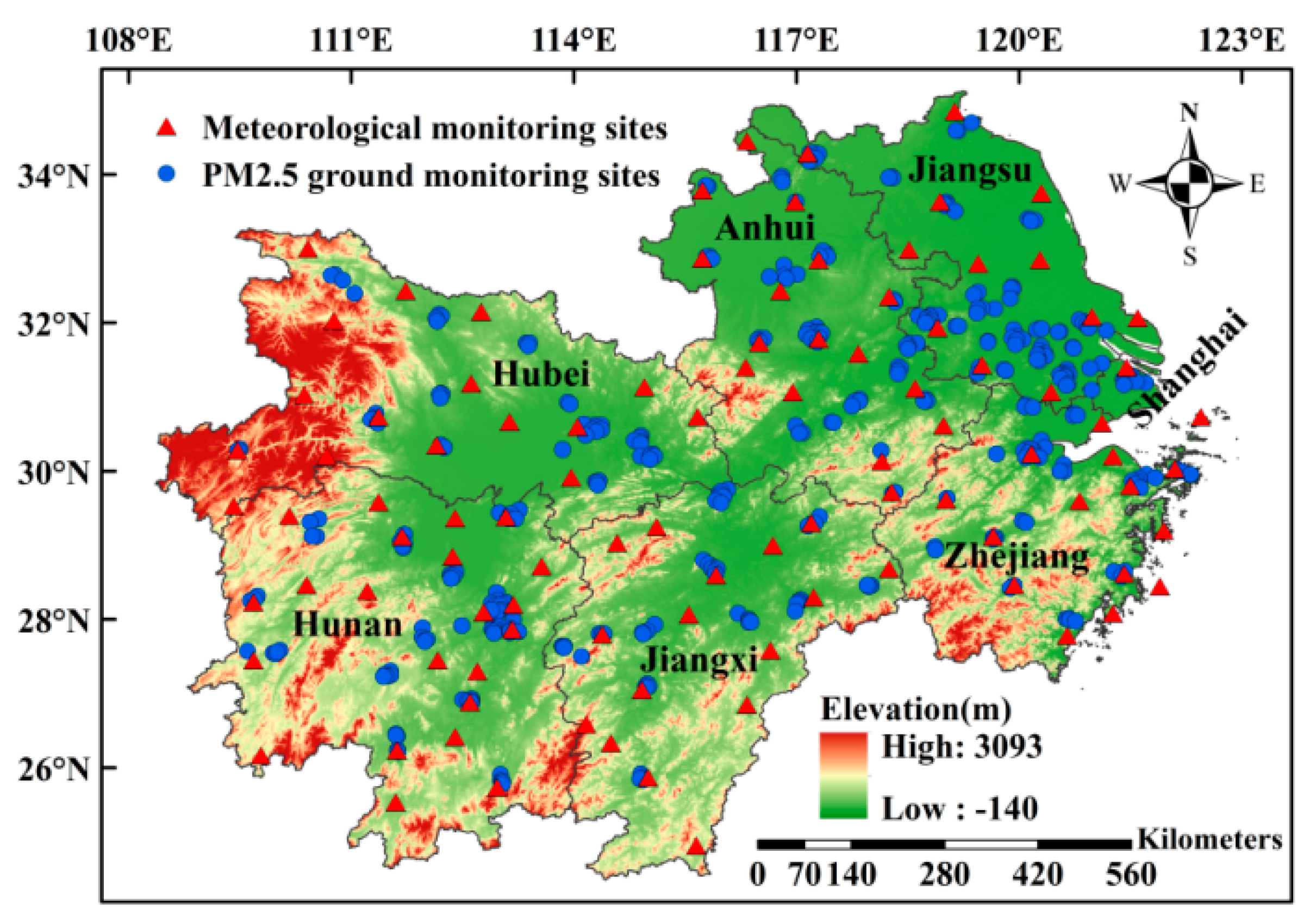
2.1. Study Area and Data Preprocessing

The middle and lower reaches of the Yangtze River Economic Belt (hereinafter collectively referred to as the middle and lower reaches of the Yangtze River) span the central-eastern region of China, located between 24°29′–35°08′N latitude and 108°21′–123°10′E longitude, and comprise six major provinces and one municipality directly under the Central Government (the lower reaches include Shanghai, Jiangsu, Zhejiang and Anhui, and the middle reaches include Jiangxi, Hubei, and Hunan). This region is one of the most developed economic regions in China. It accounts for more than a quarter of the Chinese population and approximately one-third of the Chinese gross domestic product (GDP). The Yangtze River Economic Zone has important ecological value, strong comprehensive strength, and great development potential; promoting the development of the Yangtze River Economic Zone is important for China’s economic development. However, with the economic growth of the Yangtze River Economic Zone, increases in population and motor vehicles, coupled with a regional consumption structure dominated by coal, cause severe air pollution, especially in the middle and lower reaches of the Yangtze River. This pollution has become the focus of air environment management and has received widespread public attention.
PM2.5 is the main indicator of air pollutants. To support China’s pollution prevention and control battle and ecological environmental protection strategy, we take the monthly average PM2.5 concentration data collected from PM2.5 ground monitoring stations in the middle and lower reaches of the Yangtze River economic belt for 2018–2020 as the research object.
Atmospheric pollutant (PM2.5, O3, CO, NO2, SO2) data were obtained from PM2.5 ground monitoring station observations (data from http://envi.ckcest.cn/environment/, accessed on 14 June 2022), meteorological data were obtained from meteorological monitoring station observations (data from http://data.cma.cn/, accessed on 14 June 2022), and elevation (ELE) data were obtained from the SRTMDEMUTM 90 M resolution digital elevation data product of the Geospatial Data Cloud (data from https://www.gscloud.cn/sources, accessed on 3 July 2022). The elevation, air quality monitoring station, and meteorological monitoring station distribution map is shown in Figure 1.
ZWD is the wet component of the ZTD due to water vapor in the atmosphere [43,44]. ZTD is a signal propagation delay formed by the bending and delay of electromagnetic wave signals emitted by Global Navigation Satellite System (GNSS) [45] satellites as they traverse the troposphere due to the influence of atmospheric refraction [46,47]. The ZWD data used in the experiments were obtained from the VMF data server platform (https://vmf.geo.tuwien.ac.at/, accessed on 7 May 2022).
The normalized difference vegetation index (NDVI) is one of the important parameters to reflect crop growth and nutrient information, which can detect vegetation growth and vegetation cover and reflect the background influence of the plant canopy [48,49]. The NDVI data used in the experiment were obtained from the Data Center for Resource and Environmental Sciences, Chinese Academy of Sciences (http://www.resdc.cn/, accessed on 10 December 2021); the population size (POP) data were obtained from the Worldpop website (https://hub.worldpop.org/, accessed on 3 July 2022). Table 1 indicates the time scale of each variable and access to information on the type and spatial resolution of these variables.
From Figure 1, we can see that the number of meteorological monitoring stations is smaller than the number of PM2.5 concentration monitoring stations, and ZWD is grid data. To ensure the smooth implementation of the subsequent experiments, we use the IDW method to spatially interpolate the meteorological data (TEM, PRS, WS, RH) and ZWD to obtain the corresponding raster data [17,34]. Figure 2 shows the root-mean-square error of the cross-validation results of the IDW interpolated meteorological and ZWD data.
From Figure 2, we can see that the RMSEs of meteorological factors (TEM, PRS, WS, RH) for 2018–2020 all remain within a range of intervals with small and relatively stable values, indicating the good applicability and stability of the spatial interpolation effect of IDW on meteorological factors. For the problem of large differences in the RMSE of ZWD data in different months, we found that this situation was caused by large differences in the values of ZWD in different months. The difference between the mean size of ZWD in June–August and the mean size of ZWD in December, January, and February was nearly 4 times, while the differences between the mean values of meteorological factors in different months were all less than 1 time. Therefore, the interpolation accuracy of the IDW method for ZWD is high relative to the size of ZWD and can be used for subsequent studies.
After obtaining the meteorological factor raster and ZWD raster with higher accuracy using the IDW method, we extracted the values of all raster data to the corresponding PM2.5 ground monitoring points using the spatial analysis tool of ArcGIS 10.4 software to obtain explanatory variables with a uniform spatial and temporal scale with PM2.5 data.

2.2. Methods

2.2.1. GWR Model

The geographically weighted regression (GWR) model is a spatial analysis technique that embeds the spatial location of the data into the linear regression equation based on the traditional linear regression model. Since it takes into account the local effects of spatial objects, it can better explain the spatial heterogeneity and spatial autocorrelation problems that exist in spatial data and has a high estimation accuracy. The principle of the GWR model is as follows [29,30,31,32,33,34]:
F i = β 0 ( u i , v i ) + k = 1 p β k ( u i , v i ) x i k + ε i
where F i is the observed value of the sample point and is used as the dependent variable in the GWR model. ( u i , v i ) are the coordinates of the i-th sample point, β k ( u i , v i ) is the i-th regression coefficient on each sample point, x i k is the k-th explanatory variable of the i-th observation point, p is the total number of explanatory variables, ε i is the regression residual, and β 0 ( u i , v i ) is the regression intercept term of the model at the i-th sample point.
The weighted least squares method was used to estimate the model regression coefficients; the coefficient matrix for each point is as follows:
β ( u i , v i ) = [ X T W ( u i , v i ) X ] 1 X T W ( u i , v i ) Y
where W ( u i , v i ) is the diagonal matrix of spatial weights, X is the design matrix of independent variables, and Y is the matrix of dependent variables.
The spatial weight matrix W is calculated using the bi-square function:
w i j = { ( 1 d i j 2 / θ 2 ) 2 , d i j < θ 0 , d i j > θ
where w i j is the weight between the spatially known points j and the points i to be estimated, d i j is the Euclidean distance between the points i to be estimated and the sample points j , and θ is the bandwidth size, which is judged using corrected Akaike information criterion (AICc); when A I C c is smallest, the bandwidth of the chosen weight function is optimal.

2.2.2. PCA-GWR Model

PCA is a statistical method to effectively reduce the spatial dimensionality of data that can explore the trend of multiple variables and convert multiple potential explanatory variables into new, mutually independent linear combinations of variables to replace the original variables, where the new combinations are also called principal components. The number of extracted principal components needs to be determined by the contribution of the principal components to the explanation of the variables to generally extract several principal components with a cumulative contribution of 90% or more; otherwise, the number of principal components should be adjusted [40,41,42]. PCA is primarily accomplished through the integration tools of the Scientific Platform Serving for Statistics Professional 2021. SPSSPRO (Version 1.0.11) (Online Application Software). (Retrieved from https://www.spsspro.com, accessed on 13 July 2022).
The PCA-GWR model is a combinatorial optimization model, which is based on the principle of using the PCA method to extract the principal components as new independent variables, instead of the original independent variables, to establish the modified GWR model; it not only fully considers the contribution of all potential explanatory variables to the changes in the dependent variable but also effectively addresses multicollinearity among explanatory variables. The main processes are as follows:
  • Step 1: The data of the independent variables of the GWR model were standardized, then the Kaiser-Mayer-Olkin (KMO) test and Bartlett’s test of sphericity were performed on the data. If the KMO value was greater than 0.5 and the p-value of Bartlett’s test of sphericity was less than 0.05, there was a strong correlation between the independent variables, and PCA can be performed; otherwise, the data are not suitable for PCA [50].
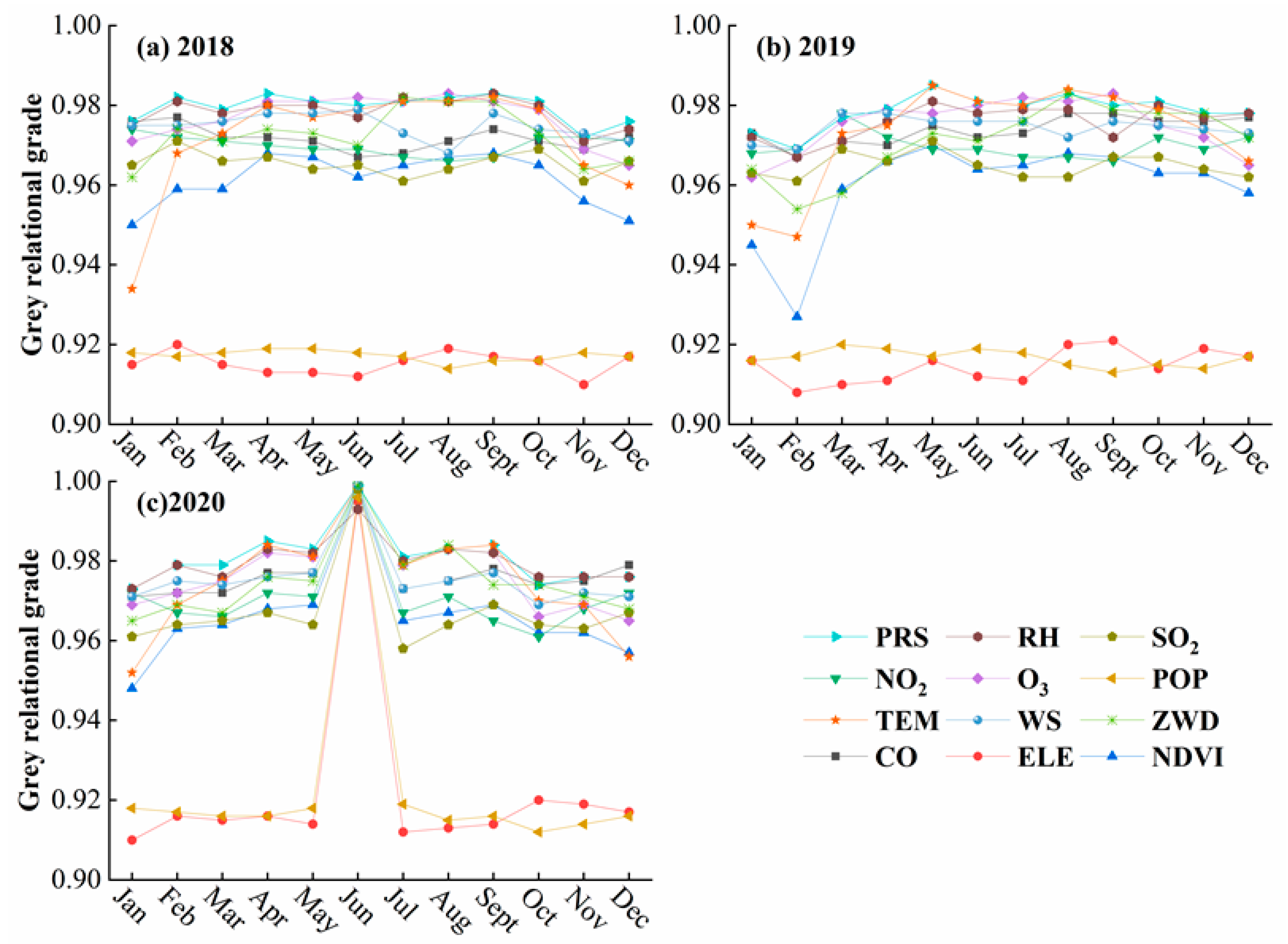
  • Step 2: The correlation between PM2.5 and the independent variable data was analyzed using the gray relation analysis (GRA) [51] integrated tool in SPSSPRO to obtain the gray correlation value, and the closer the gray relational grade was to 1, the higher the correlation between the variable and PM2.5.
  • Step 3: The variables with high correlation (gray relational grade >0.9) were selected as input variables for PCA, and all principal components were calculated using the PCA integration tool in SPSSPRO.
  • Step 4: All the principal components were ranked and cumulatively summed according to the percentage of variance, and those with a cumulative percentage of variance greater than or close to 90% were selected as the final input variables of the GWR model. The PCA-GWR model was then constructed to obtain the estimation results of the target variables.

2.2.3. RBF Interpolation

Radial basis function interpolation (RBF) is an accurate deterministic spatial interpolation method that makes no assumptions about the data and provides accurate prediction surfaces, which is beneficial for dealing with scattered data and approximating surfaces. In addition, it can interpolate predicted values larger than the maximum and smaller than the minimum of the observed values when the maximum and minimum of the spatial data are not clear, and it has the advantages of simple computational format, flexible node configuration, small computational effort, and relatively high accuracy. The RBF interpolation during this research was implemented using the RBF interpolation analysis tool in the geostatistical analysis toolkit of ArcGIS 10.4 software [52]. The basic principle of the model can be expressed as follows [53,54]:
Z ^ ( x , y ) = i n λ i φ ( r i ) + T ( x , y )
where ( x , y ) are the coordinates of the points to be interpolated, n is the number of sample points, λ i is the weight coefficient obtained by solving the linear system of equations, φ ( r i ) is the basis function, and T ( x , y ) = a + b x + c y is the trend function.
The coefficients of the trend function T ( x , y ) are solved using the least squares method, and the following constraints must be satisfied when solving:
{ i = 1 n λ i = 0 i = 1 n λ i T ( x i , y i ) = 0
where ( x i ,   y i ) are the coordinates of the sample points i .
The basis functions of the RBF are chosen from the Completely Regular Spline (CRS) function: ϕ   CRS ( r i ) ; the Tension Sample (TS) function: ϕ   TS ( r i ) ; the Multiquadric Spline (MS) function: ϕ   MS ( r i ) ; the Inverse Multiquadric Spline (IMS) function: ϕ   IMS ( r i ) ; and the Thin Plate Spline (TPS) function: ϕ   TPS ( r i ) . The five basis functions [55] are calculated as follows:
ϕ   CRS ( r i ) = 2 ln ω r i 2 + E 0 ( ω r i 2 ) 2 + c 0
ϕ   TS ( r i ) = ln ω r i 2 + K 0 ( ω r i ) 2 + c 0
ϕ   MS ( r i ) = r i 2 + ω 2
ϕ   IMS ( r i ) = 1 r i 2 + ω 2
ϕ   TPS ( r i ) = ( ω r i ) 2 ln ( ω r i )
where r i is the Euclidean distance between the point ( x , y ) to be interpolated and the i-th sample point, E 0 is the exponential integration function, K 0 is the corrected Bessel function, c 0 is a constant (0.577215), ω is the smoothing factor, and the optimal smoothing factor for each basis function is automatically calculated by the parameter optimization function in the geostatistical analysis tool of ArcGIS 4.0.

2.2.4. Combined Model with Residual Correction Based on the RBF Interpolation

The PCA-GWR model is an inaccurate spatial interpolation method, and its estimated value at a known location is not equal to the known value; hence, the residual interpolation correction of the estimated value of the PCA-GWR model can be used to further improve the accuracy of PM2.5 estimation. In addition, due to the diverse and complex influencing factors of PM2.5, the PCA-GWR model cannot fully explain the spatial variation of PM2.5, which means the residuals of the model will have some spatial autocorrelation; hence, the spatial interpolation method can be considered to correct the residuals of the PCA-GWR model to further explain the spatial characteristics of PM2.5.
Therefore, based on these two considerations of the PCA-GWR model, five radial basis function (RBF) interpolation methods based on different basis functions (CRS, TPS, IMS, IM, TS) are selected to interpolate the residuals of the PCA-GWR model to further optimize the interpolation accuracy of the model, and five residual correction models (PCA-GWRCRS, PCA-GWRTS, PCA-GWRMS, PCA-GWRTPS, PCA-GWRIMS) are constructed. Their model principles are described as follows:
F PCA - GWRRBF   = F ^ PCA - GWR + Z RES   ( RBF )
where F PCA - GWRRBF denotes the value after residual RBF interpolation correction for the estimated values of the PCA-GWR model, F ^ PCA - GWR denotes the estimated value of the PCA-GWR model, and Z RES   ( RBF ) denotes the residual estimates obtained after the RBF interpolation of the regression residuals of the PCA-GWR model. The subscript RBF indicates five different RBF spatial interpolation methods (CRS, TS, MS, TPS, IMS).

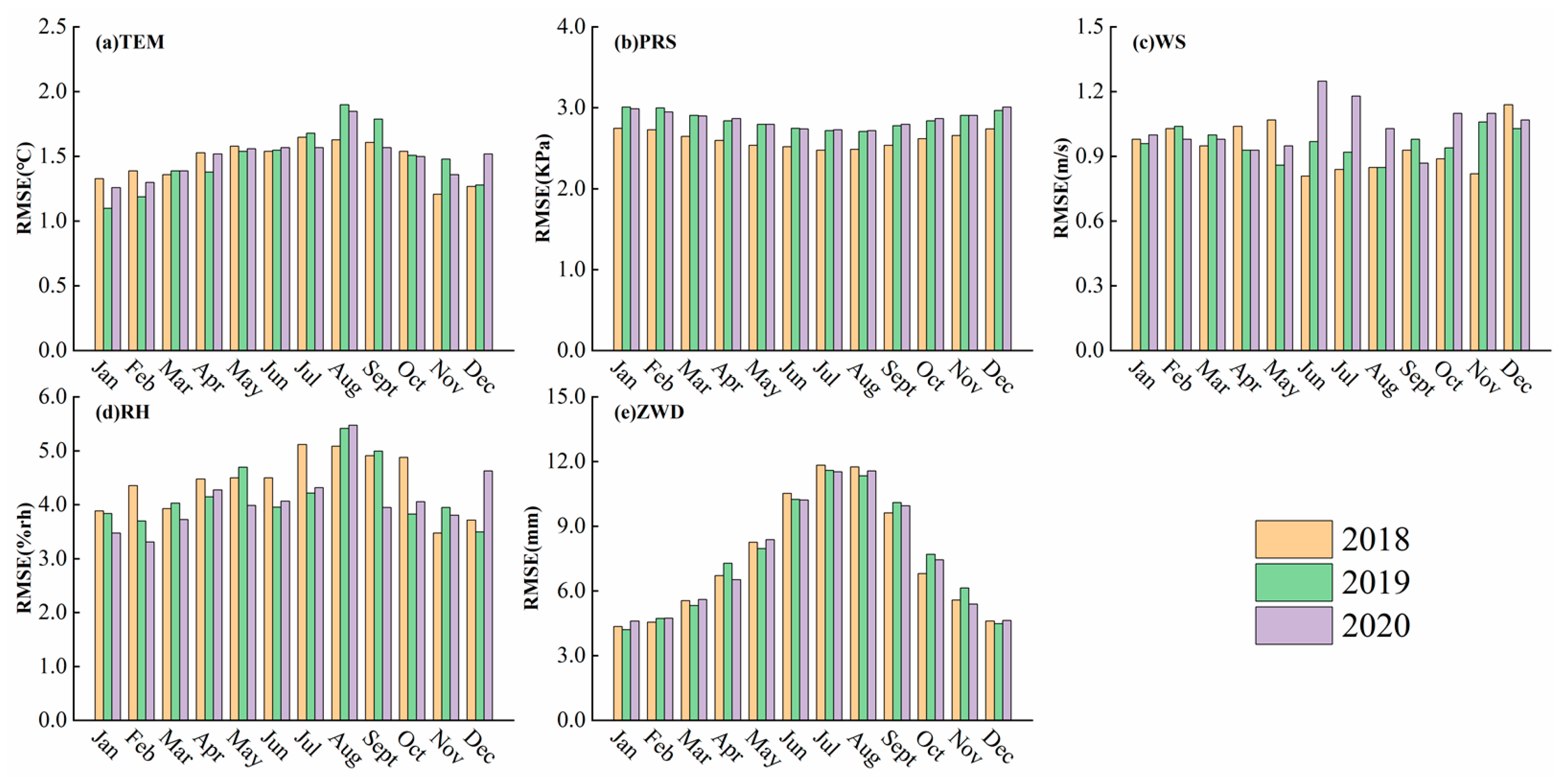
2.2.5. Evaluation Indicators

To evaluate the model accuracy more intuitively, we use four metrics, the root mean square error (RMSE), mean absolute error (MAE), mean absolute percentage error (MAPE), and the decidability Factor R2, to comprehensively evaluate the model’s accuracy and performance.
R M S E = 1 n i = 1 n ( x i x ^ i ) 2
M A E = 1 n i = 1 n | x i x ^ i |
M A P E = 100 % n i = 1 n | x i x ^ i x i |
R 2 = i ( x ^ i x i ) 2 i ( x ¯ x i ) 2
where n is the total number of samples, x i is the observed value of the target variable at the i-th position, x ^ i is the estimated output of the model at the same position, and x ¯ i is the average value of the total number of samples.
In general, RMSE and MAE are mainly used to evaluate the estimation accuracy of the model, and the smaller the value is, the higher the estimation accuracy of the model and vice versa. MAPE and R2 are mainly used to evaluate the performance of the model, and the smaller the value of MAPE and the closer the value of R2 is to 1, the better the performance and fitting effect of the model and vice versa.

3. Results

3.1. Analysis of PM2.5 and Its Related Explanatory Variables

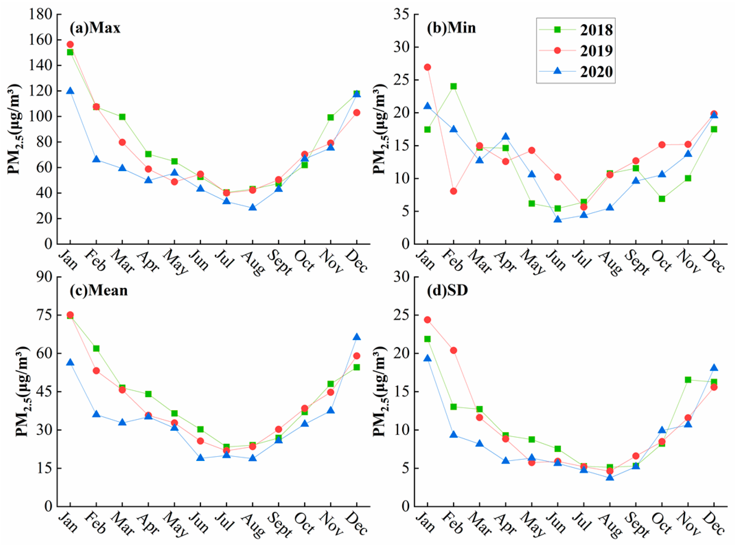
3.1.1. PM2.5 Descriptive Statistics

To further understand the change in PM2.5 concentration in January–December 2018–2020, we conducted descriptive statistics on PM2.5 ground monitoring station data, and the results are shown in Figure 3.
From Figure 3, it can be seen that the maximum (Figure 3a), minimum (Figure 3b), mean (Figure 3c), and standard deviation (Figure 3d) of PM2.5 concentrations in January–December 2018–2020 show a ‘U’-shaped distribution; therefore, it can be concluded that PM2.5 concentrations are high in December, January, and February, low in June–August, and moderate in March–May and September–November each year. In addition, the standard deviation of PM2.5 concentrations in December, January, and February of 2018–2020 is greater than that of the remaining months, indicating that the PM2.5 data for December, January, and February are more discrete and less stable, while the data for the remaining months are more stable.

3.1.2. GRA

To ensure that both PCA and GWR models have good modeling effects and that subsequent tests were carried out smoothly, we used the GRA method to analyze the correlation between PM2.5 and 12 explanatory variables and measured the correlation between the two variables by the closeness of the gray relational grade to 1 [56]. The GRA results are shown in Figure 4.
From Figure 4, it can be concluded that the gray relational grade between PM2.5 and the 12 explanatory variables (CO, NDVI, NO2, O3, PRS, RH, SO2, TEM, WS, ZWD, ELE, and POP) are all greater than 0.9, whereas the gray relational grade with ELE and POP is lower than other variables, and the highest gray relational grade is with PRS; the gray relational grade in 2018–2019 showed a slow trend of increasing and then decreasing on the monthly scale. In summary, PM2.5 has a high correlation with all 12 explanatory variables, which can be used as input variables for the construction of GWR and PCA models.

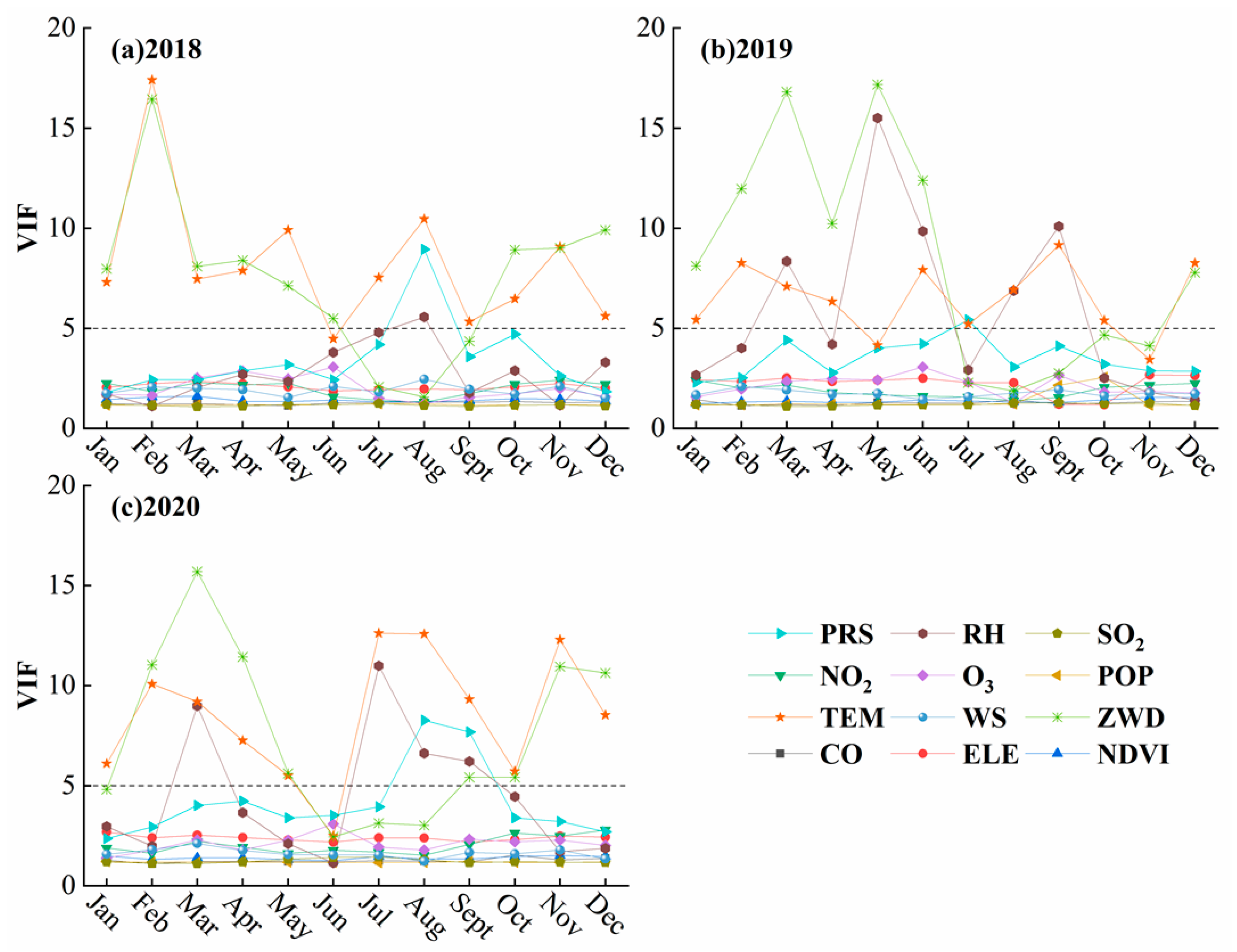
3.1.3. Multicollinearity Diagnosis
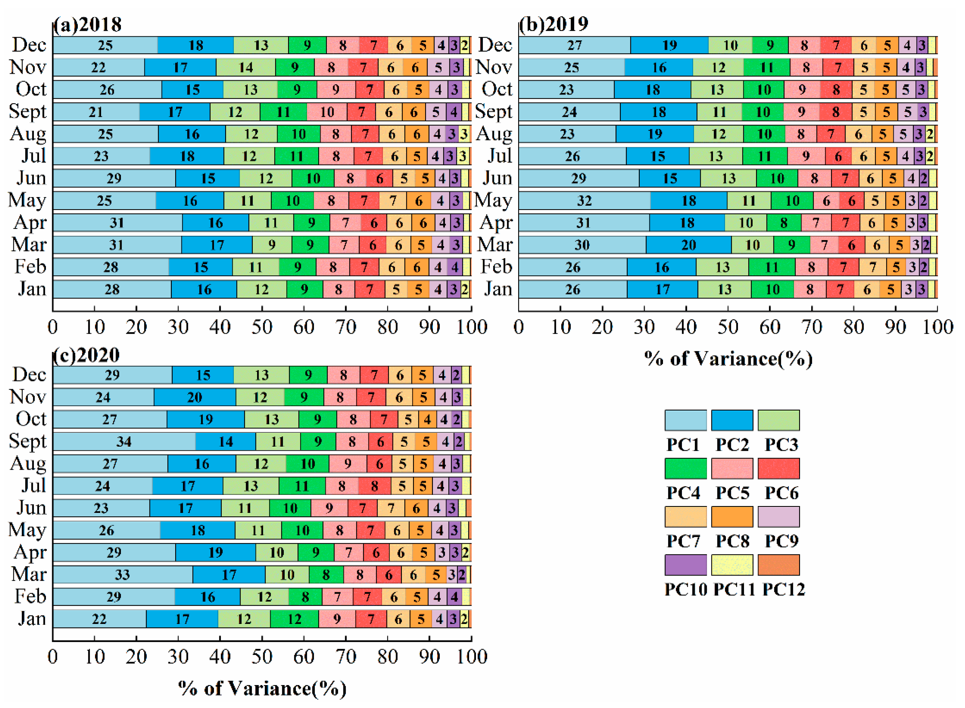
Multicollinearity refers to the distortion of model estimates due to the correlation between explanatory variables in a linear regression model; it is necessary to test for multicollinearity among explanatory variables before constructing a GWR model. Selecting a combination of variables suitable for modeling based on the diagnostic results can ensure the accuracy of model estimation. Therefore, the exploratory regression method in the spatial statistics tool of ArcGIS 4.0 is used to test the multicollinearity among the 12 explanatory variables and judge the severity of multicollinearity by the magnitude of the output variance inflation factor (VIF) value. The closer the VIF value is to 1, the lighter the multicollinearity among the variables, and the greater the VIF value is than 1, the more severe the multicollinearity between variables. If the VIF value is between 1 and 5, then the multicollinearity among the explanatory variables is mild and the impact on the estimation accuracy of the regression model is negligible. If the VIF value is greater than 5, then the multicollinearity among the explanatory variables is more serious, the impact on the estimation accuracy of the model is not negligible, and a reasonable method must be used to address it [57,58]. The results of the diagnosis of multicollinearity among the explanatory variables are shown in Figure 5.
From Figure 5, it can be seen that there are varying degrees of multicollinearity (VIF > 5) between the explanatory variables for PM2.5 in most months of 2018–2020, with TEM (February, May, and August 2018 (Figure 5a); February, July, August, and November 2020 (Figure 5c)), ZWD (February and December 2018 (Figure 5a); February–June 2019 (Figure 5b); February, March, April, November, and December 2020 (Figure 5c)), and RH (May and September 2019 (Figure 5b); July 2020 (Figure 5c)) causing the highest likelihood of multicollinearity (VIF > 10). However, the VIF between the explanatory variables for PM2.5 in June 2020 and November 2019 is less than 5, indicating that the multicollinearity between the explanatory variables for PM2.5 in these two months is small.
Therefore, to minimize the multicollinearity among the explanatory variables of PM2.5 and obtain the best combination of explanatory variables suitable for PM2.5 estimation in all months, we screened and excluded the explanatory variables with large VIFs and performed stepwise multicollinearity diagnosis. The results show that in months with more severe multicollinearity (VIF > 5), the VIFs of the remaining explanatory variables after excluding TEM and ZWD all decrease to varying degrees and are all less than 5. Moreover, there is a corresponding decrease in the VIF of the remaining explanatory variables in November 2019 and June 2020 after the exclusion of these two variables. In summary, we considered the use of the remaining 10 explanatory variables of PM2.5 (CO, NO2, O3, SO2, PRS, WS, RH, NDVI, ELE, and POP) to construct a GWR model for the interpolation estimation of PM2.5 spatial distribution.

3.1.4. PCA

Although the 10 explanatory variables selected by stepwise exploratory regression effectively reduced the multicollinearity among the explanatory variables, two explanatory variables (ZWD and TEM) with a high correlation with PM2.5 were excluded, and the contribution of all potential explanatory variables to the change in PM2.5 was not fully considered; hence, we chose the PCA method to reduce the dimensionality of the 12 explanatory variables to further minimize the influence of multicollinearity among the explanatory variables while maximizing the contribution of the explanatory variables to the variation in PM2.5 spatial distribution.
Before conducting principal component analysis, we conducted the KMO test and Bartlett’s test of sphericity on the explanatory variables for each month of 2018–2020. The experimental results yielded KMO values greater than 0.5 among the explanatory variables for each month of 2018–2020, and Bartlett’s test of sphericity of p-values was 0.000 *** (Note: *** represents a 1% significance level), which basically meets the requirements of principal component analysis and allows for the PCA of explanatory variables; the results of the percentage of variance of the PCA are shown in Figure 6.
As shown in Figure 6, the percentage of variance of the first principal component (PC1) for January–December 2018–2020 is between 20 and 35%, the percentage of variance of the second principal component (PC2) is between 14 and 20%, and the percentage of variance of the third principal component (PC3) and fourth principal component (PC4) is approximately 10%; the rest of the percentage of variance is below 10% and decreases with the increase in the principal component number. The cumulative percentage of variance of PC1–PC8 is approximately 90%, indicating that PC1–PC8 contributed 90% and above to the 12 explanatory variables, so we selected PC1–PC8 as the independent variables of the GWR model and constructed the PCA-GWR model for PM2.5 spatial distribution estimation.

3.2. Model Regression

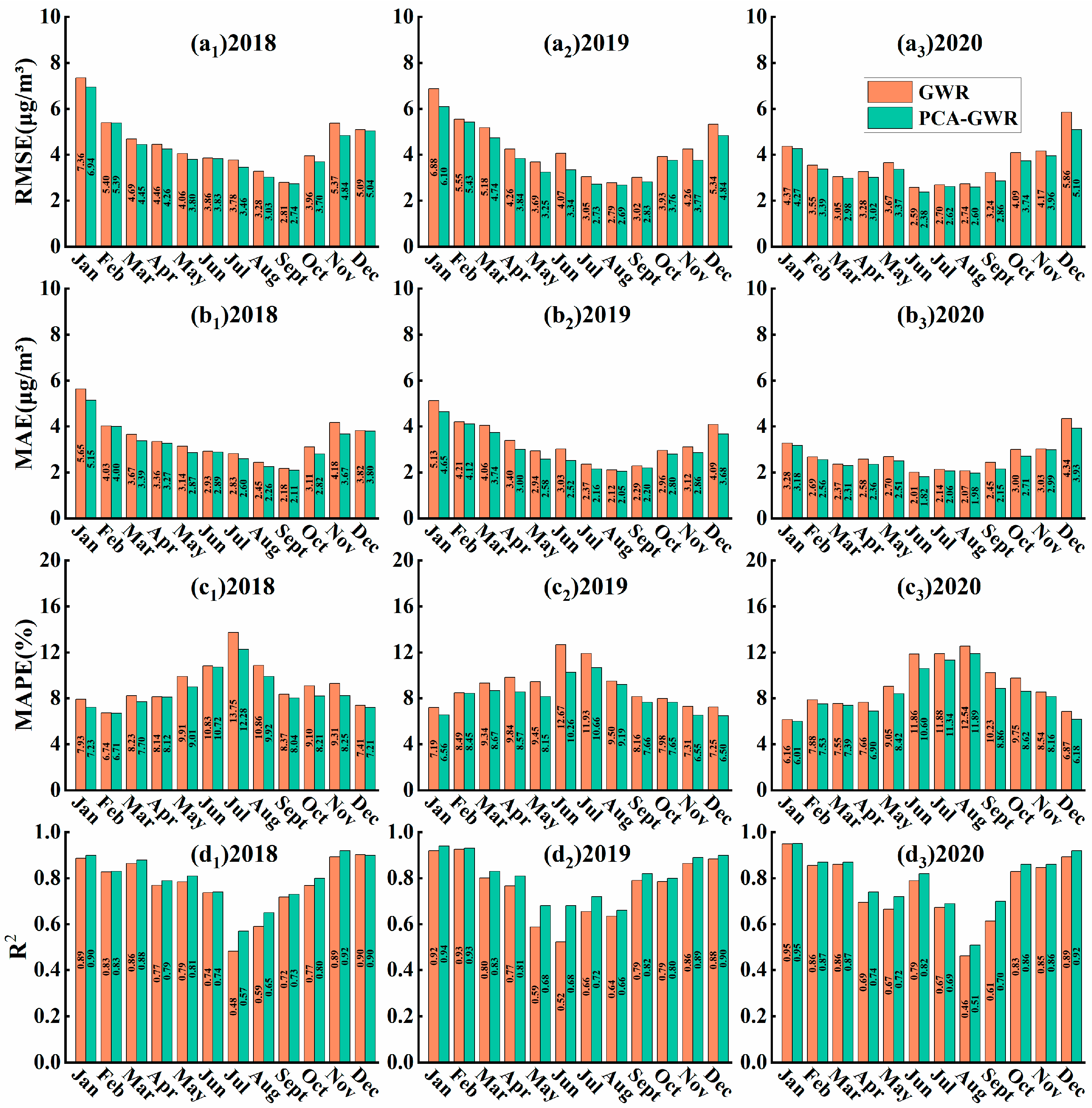
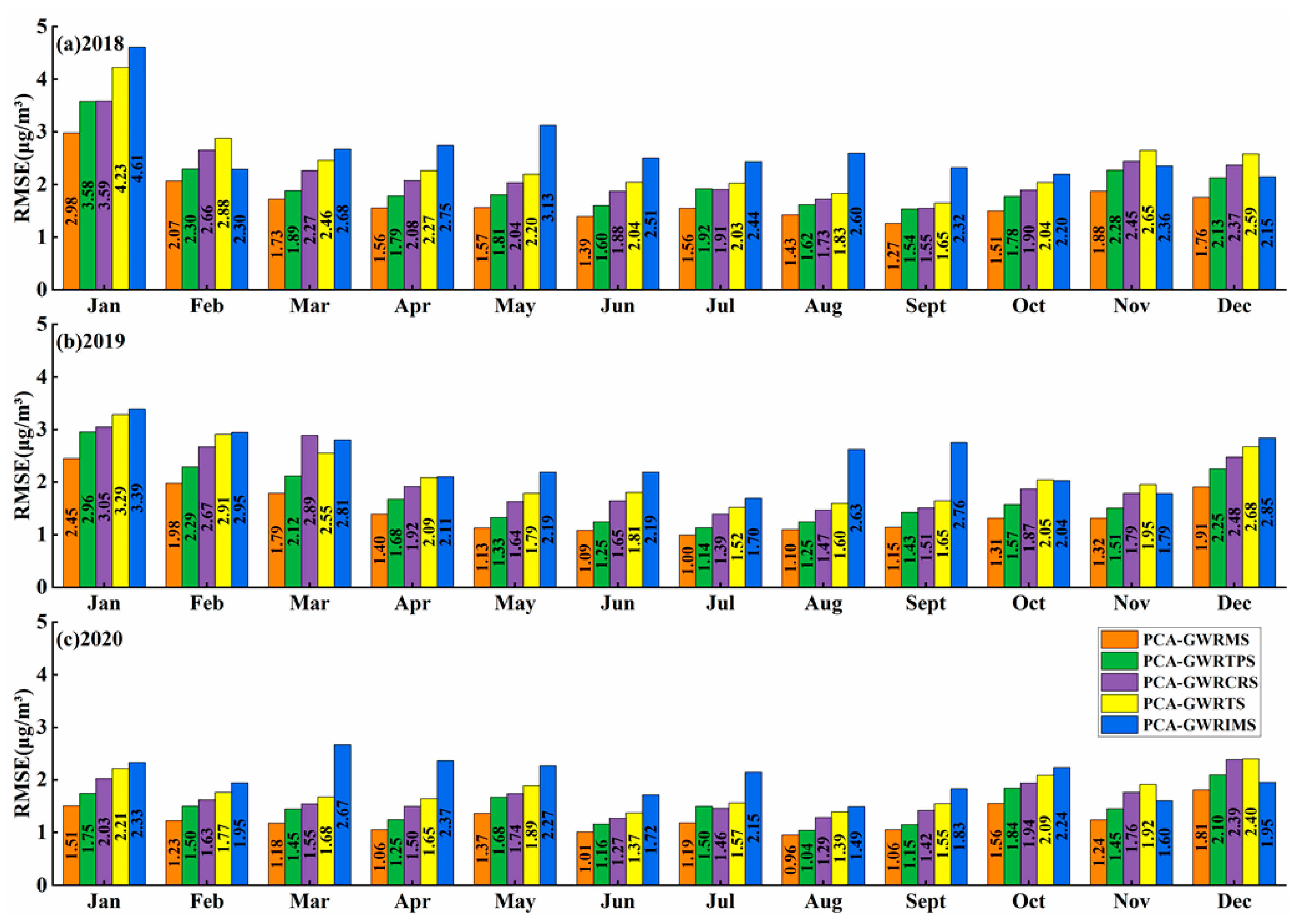
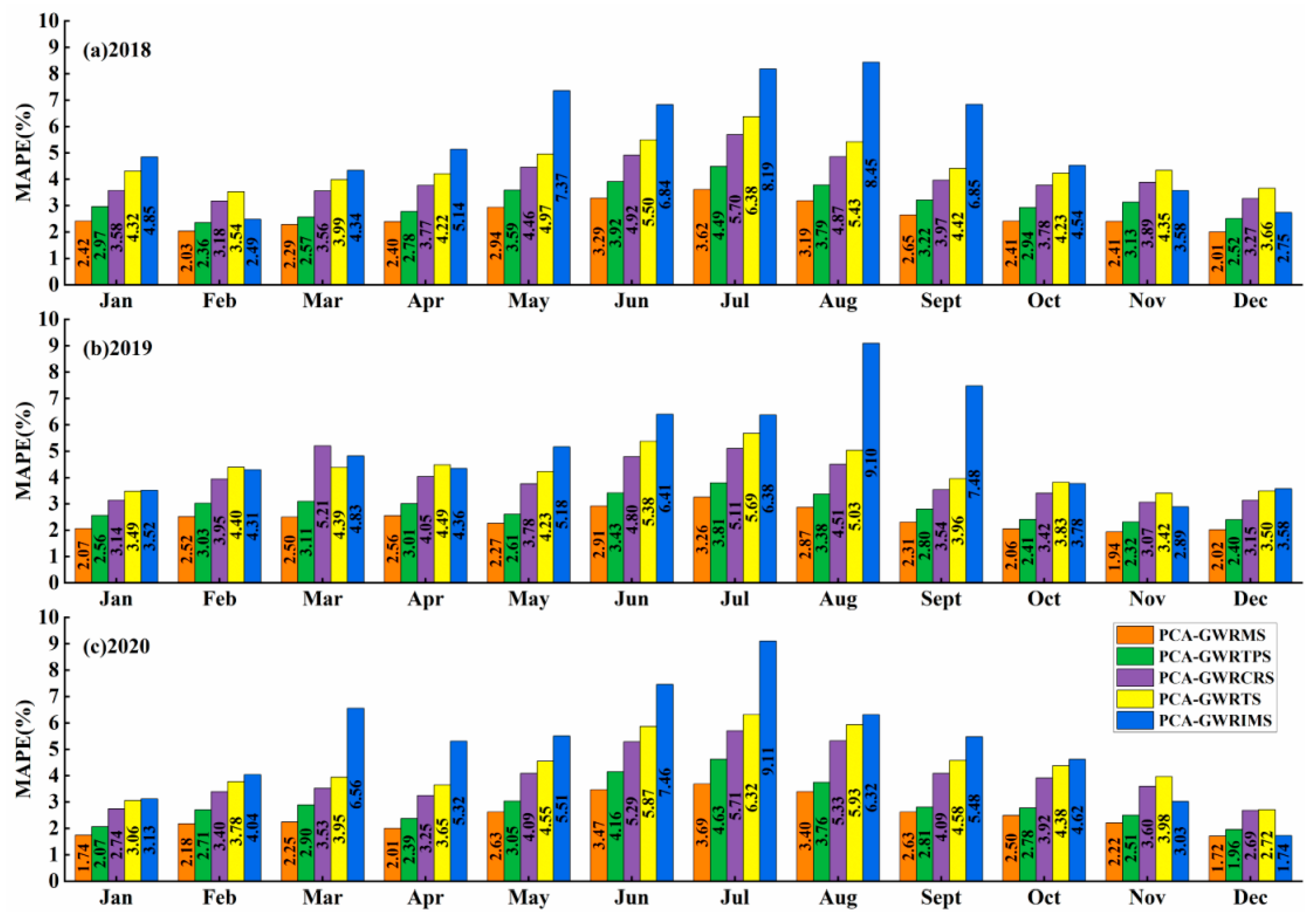
3.2.1. Comparison of Model Accuracy

Through a series of exploratory analyses, we finally selected 10 variables (CO, NO2, O3, SO2, PRS, WS, RH, NDVI, ELE, and POP) to construct the GWR model and selected principal component analysis to extract the eight principal components, whose cumulative contribution to the 12 explanatory variables was nearly 90%, to construct the PCA-GWR model and compared the accuracy and model performance of the two models, the results of which are shown in Figure 7.
Comparing Figure 7a1–a3,b1–b3, it can be seen that the RMSE of both the GWR and PCA-GWR models is less than 8 μg/m3 and the MAE values are less than 6 μg/m3 for the monthly average PM2.5 estimation from 2018 to 2020, which indicates that both models have higher accuracy in estimating PM2.5 concentrations. In addition, the RMSE and MAE of the PCA-GWR model generally improved to different degrees compared with the GWR model, with the RMSE of November 2018, June 2019, September 2020, and December 2020 improving significantly compared with the GWR model by 9.89%, 17.94%, 11.59%, and 12.98%, respectively. The MAEs in November 2018, June 2019, September 2020, and December 2020 were more significantly optimized relative to the GWR model, with improvements of 12.20%, 16.86%, 12.20%, and 9.51%, respectively; therefore, it can be concluded that the spatial estimation accuracy of the PCA-GWR model for PM2.5 is better than that of the GWR model.
From Figure 7c1–c3,d1–d3, it can be seen that the MAPE of the PCA-GWR model is smaller than that of the GWR model in 2018–2020, where the improvement of MAPE relative to the GWR model is more obvious in November 2018, June 2019, September 2020, and December 2020, with 11.39%, 19%, 11.63%, and 10.11%, respectively, in that order. The MAPE of the PCA-GWR model remains between 10 and 13 in June–August and is less than 10 in the rest of the months, with the smallest MAPEs in February 2018, December 2019, and January 2020. Meanwhile, the R2 of the PCA-GWR model is larger than that of the GWR model, among which the R2 values in July 2018, June 2019, and September 2020 are more significantly improved relative to the GWR model by 15.79%, 23.53%, and 12.86%, respectively, in that order. The R2 of the PCA-GWR model is larger in January–March and October–December than in April–September, among which the PCA-GWR model had R2 values greater than 0.9 in January, November, December 2018–2019, and January and December 2020.
In summary, compared with the GWR model, the PCA-GWR model can not only fully consider the contribution of all potential explanatory variables to the PM2.5 changes and minimize the multicollinearity among explanatory variables, but also effectively improve the precision and fitting effect of the spatial estimation of PM2.5; hence, it is feasible to optimize the GWR model using principal component analysis. However, the fitting effect and estimation accuracy for some months are still relatively poor, so we subsequently considered the residual correction process of the PCA-GWR model using the spatial interpolation method to further improve the estimation accuracy and fitting effect of PM2.5.

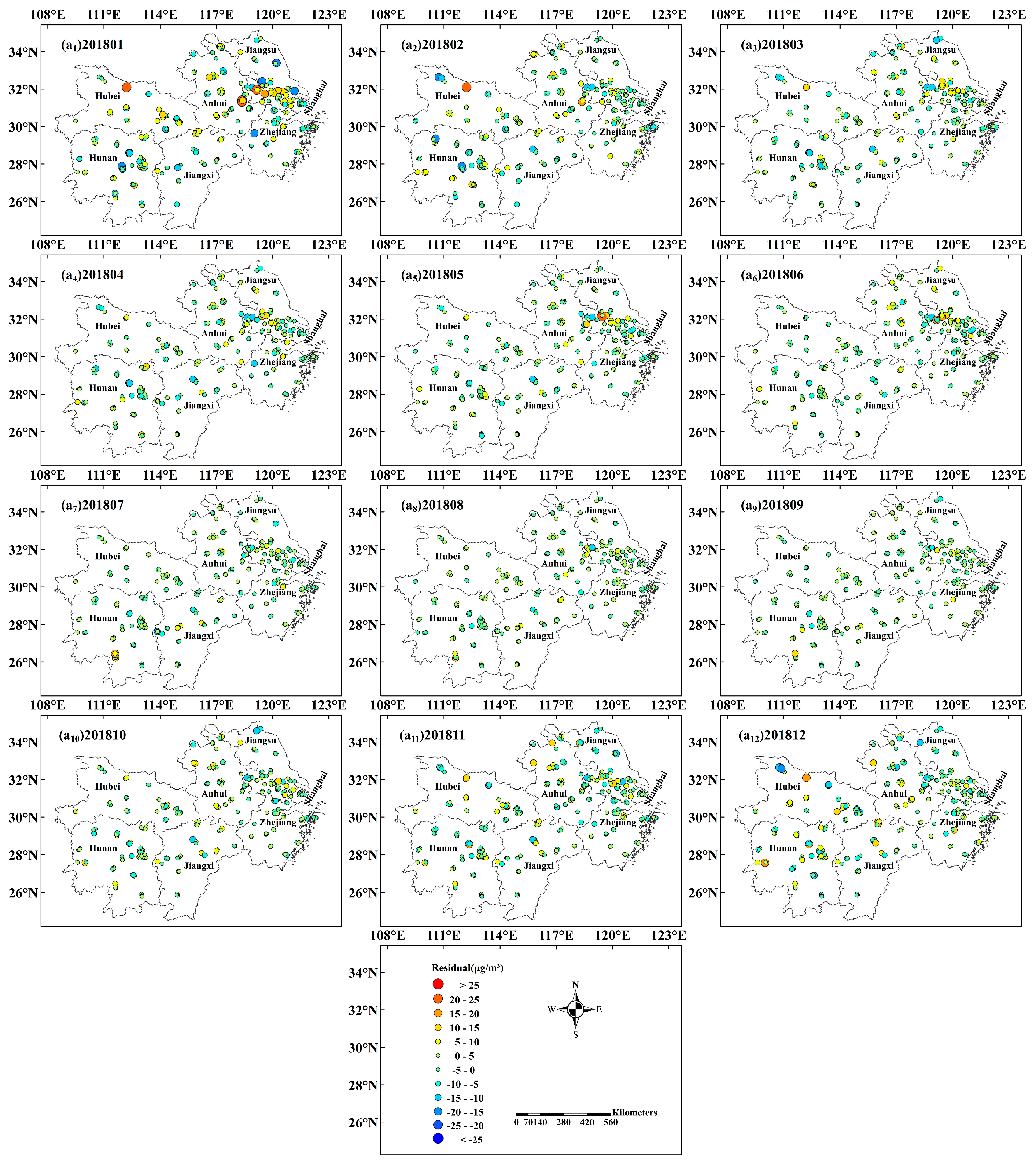
3.2.2. Regional Distribution of Model Residuals

From Figure 7, we know that the model performance and estimation accuracy of PCA-GWR are better than those of the GWR model, but the estimation accuracy and fitting effect of the PCA-GWR model still have room for improvement, so the spatial distribution of the residuals of the PCA-GWR model is visualized to further analyze the spatial distribution pattern of the residuals of the PCA-GWR model.
Since the strengths and weaknesses of the model interpolation effects for 2018–2020 are basically the same, we use the spatial distribution of residuals of the PCA-GWR model for January–December 2018 in the middle and lower reaches of the Yangtze River (Figure 8a1–a12) as an example to save space and use these plots as the basis for our analysis.
From Figure 8, it can be seen that the residual distribution of the PCA-GWR model shows a spatial trend of high in the north and low in the south, and the absolute values of residuals greater than 20 μg/m3 are mainly concentrated in January, February, and December. When we combine these data with Figure 7, we can see that although the residuals in January, February, and December 2018 are larger, their MAPEs are less than 10 and their R2 values are greater than 0.8, indicating that the PCA-GWR model has a better fit for PM2.5, but there is still room for optimizing the estimation accuracy of the model. When we combine PM2.5 values with Figure 3, it can be seen that the PM2.5 concentrations in June–August 2018 are lower than those in other months, but the absolute value of the residuals from June to August is large in relation to the ratio of PM2.5 concentration, thus making the MAPE of the PCA-GWR model in June, July, and August large and the R2 small (Figure 7).
In summary, although the accuracy and fitting effect of the PCA-GWR model are better than those of the conventional GWR model, there is still room for optimizing the residuals of the PCA-GWR model for estimating PM2.5 concentrations in months with high and low PM2.5 concentrations; therefore, residual correction for the PCA-GWR model can be considered.

3.2.3. Residual Correction of PCA-GWR Model

To ensure the smooth process of introducing spatial interpolation methods for the residual correction of PCA-GWR models in subsequent experiments, we performed a spatial autocorrelation analysis on the regression residuals of the PCA-GWR model. The experiments were performed by calculating the global Moran’s I spatial autocorrelation of the residuals of the PCA-GWR model with the spatial analysis tool of GeoDa version 1.18.0 software; the results are shown in Table 2.
As seen from Table 2, the residuals of the PCA-GWR model for most months of 2018–2020 are spatially autocorrelated, their p-values are almost all less than 0.1, and the absolute values of the Z values are almost all greater than 1.65, indicating that the spatial autocorrelation of the residuals of the PCA-GWR model is significant at the 0.1 level with a confidence level greater than 90%, and the spatial autocorrelation of the residual results are generated by random processes with less than 10% chance.
Therefore, we introduce five different radial basis function (CRS, TS, MS, IMS, TPS) interpolation methods to correct the residuals of PCA-GWR models and construct five improved models (PCA-GWRCRS, PCA-GWRTS, PCA-GWRMS, PCA-GWRIMS, PCA-GWRTPS). The evaluation of the interpolation accuracy of the leave-one-out cross-validation method for the five improved models is shown in Figure 9 and Figure 10.
As seen from Figure 9 and Figure 10, the estimation accuracy and fitting effect of the five models for PM2.5 after residual correction have all improved and enhanced to different degrees relative to the PCA-GWR model, among which the RMSE and MAPE of the PCA-GWRMS model have improved most significantly compared to the PCA-GWR model. For the PCA-GWRMS model, RMSE improved by 59.40% on average and MAPE improved by 69.37% on average in January–December 2018; RMSE improved by 62.89% and MAPE improved by 70.37% on average in January–December 2019; and RMSE improved by 61.95% and MAPE improved by 70.32% on average in January–December 2020. In addition, from the changes in RMSE and MAPE in the different months of each year, it can be concluded that the overall correction effects of the five radial basis interpolation methods on the residuals are in the order of MS > TPS > CRS > TS > IMS, where the MS interpolation algorithm effectively improves the estimation accuracy and model performance of the PCA-GWR model and creates relatively more stable interpolation effects for different months compared with other interpolation methods.
Comparing Figure 9a–c, we can see that the RMSE of all five models is less than 5 μg/m3 for each month in 2018 (Figure 9a), the RMSE value is less than 3.5 μg/m3 for each month in 2019 (Figure 9b), and the RMSE value is less than 3 μg/m3 for each month in 2020 (Figure 9c). This indicates that the interpolation accuracy of all five interpolation models for PM2.5 is high, among which the interpolation effect is the best for 2020 PM2.5 and the worst for 2018 PM2.5. Comparing Figure 10a–c, we can see that the MAPE of all five models is less than 10, among which the MAPE of both the PCA-GWRMS and PCA-GWRTPS models is less than 5, indicating that the two models have a better fitting effect and better model performance for PM2.5, while the PCA-GWRMS model is better than the PCA-GWRTPS model among the two models.
In summary, all five interpolation models (PCA-GWRCRS, PCA-GWRTS, PCA-GWRMS, PCA-GWRIMS, and PCA-GWRTPS) can better achieve the interpolation estimation of the spatial distribution of monthly PM2.5 in the middle and lower reaches of the Yangtze River for 2018–2020 with better interpolation accuracy and fitting effect, among which the PCA-GWRMS model outperformed the other four residual correction models and the PCA-GWR model in all aspects.

3.3. Generation of the Spatial Distribution Map of the PM2.5 Concentration

Through the analysis, we concluded that the accuracy and performance of the PCA-GWRMS model are better than those of the other models, and this model takes into account more comprehensive PM2.5 influencing factors and less data loss; hence, we chose to use the PCA-GWRMS model to generate the spatial distribution map of PM2.5 concentrations in the middle and lower reaches of the Yangtze River from 2018 to 2020. Its mapping steps are as follows:
  • Step 1: Based on the PM2.5 concentration of 390 ground monitoring stations, we use ArcGIS 4.0 to encrypt the PM2.5 monitoring stations and obtain 0.5° × 0.5° grid points.
  • Step 2: The inverse distance weighting (IDW) method is used to interpolate the atmospheric pollutants (CO, NO2, O3, SO2), meteorological data (TEM, PRS, WS, RH), and ZWD data to obtain the raster of the corresponding data, and then ArcGIS 4.0 is used to extract the values of the NDVI raster, ELE raster, and POP raster to the 0.5° × 0.5° grid points and 390 PM2.5 ground monitoring stations.
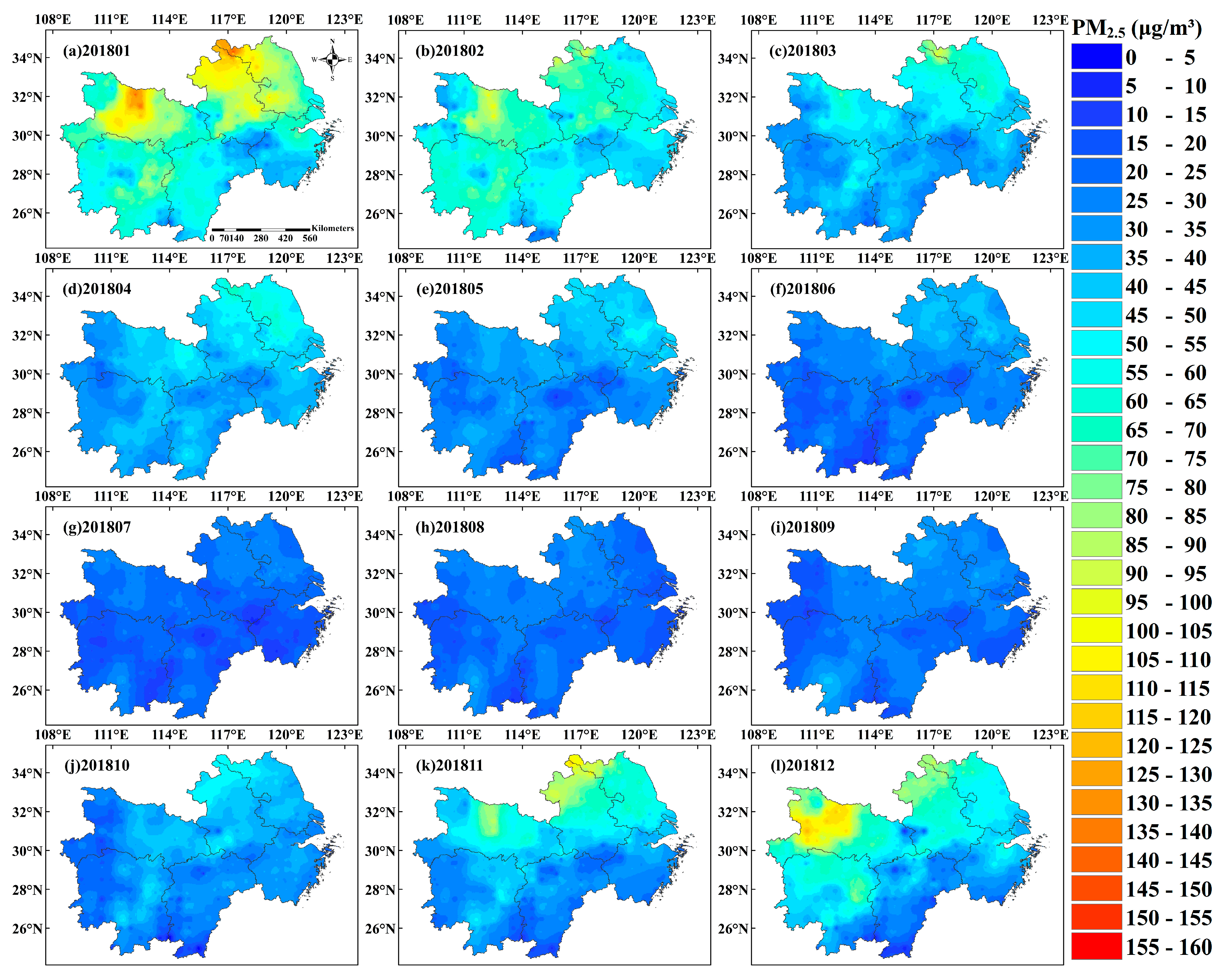
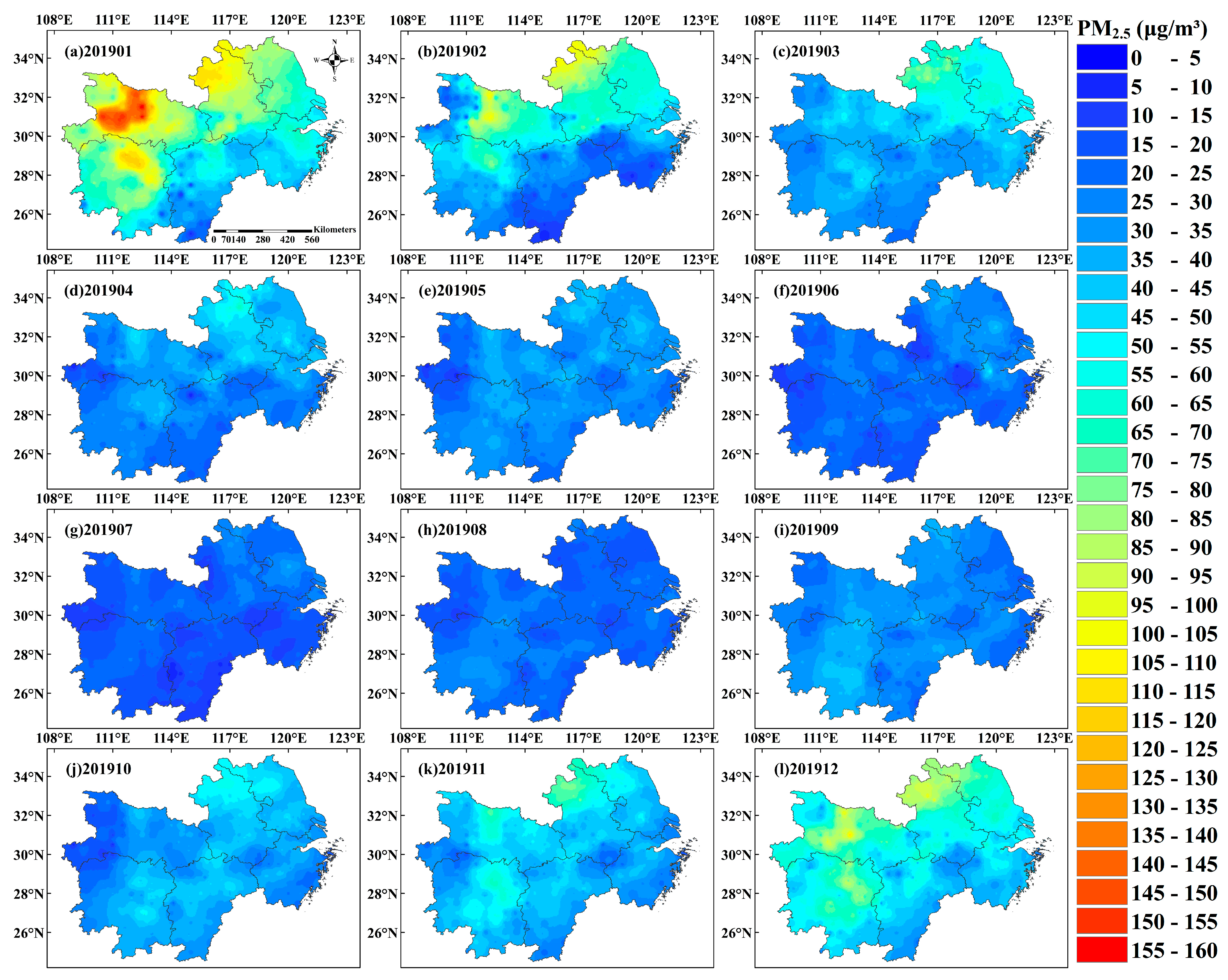
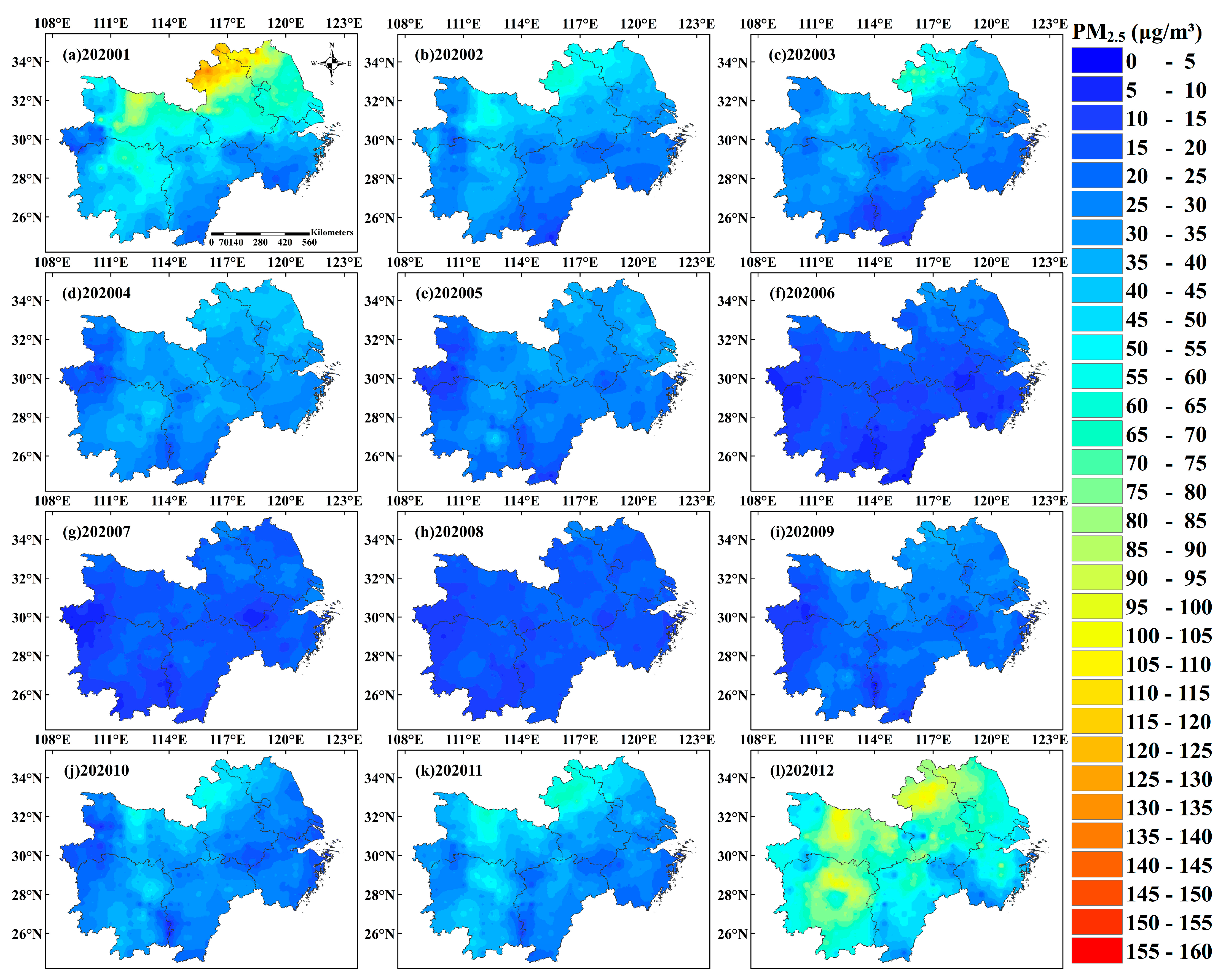
  • Step 3: We construct the PCA-GWRMS model using data from 390 monitoring stations to obtain PM2.5 estimates for 0.5° × 0.5° grid points, then visualize the predicted values for 0.5° × 0.5° grid points and the actual PM2.5 values from 390 ground monitoring stations using the inverse distance weighting (IDW) [31] interpolation method to generate a PM2.5 concentration spatial distribution map from January to December 2018–2020 (Figure 11, Figure 12 and Figure 13).
From the PM2.5 spatial distribution in Figure 11, Figure 12 and Figure 13, it can be seen that the PM2.5 concentration distribution in the middle and lower reaches of the Yangtze River in 2018–2020 has a ‘U’-shaped distribution on a monthly scale, which is consistent with the results described in Figure 3, where the PM2.5 concentrations in January, February, and December are high, and those in June, July, and August are low, especially in the northern part of the study area in January each year, which is generally higher than 75 μg/m3. From the overall PM2.5 spatial distribution, PM2.5 concentrations show a spatial trend of high in the north and low in the south, and this variation is obvious in January–March and November–December each year, indicating that the use of the PCA-GWRMS model can better estimate regional PM2.5 concentrations and generate a spatial distribution map of PM2.5 concentrations with a high degree of refinement.

4. Discussion

In this paper, we found that the distribution of PM2.5 in six provinces and one city in the middle and lower reaches of the Yangtze River in China shows a ‘U’-shaped distribution on different monthly scales, with high PM2.5 concentrations mainly occurring in winter months (January, February, and December), where PM2.5 concentrations are higher in January than in other months, and low concentrations are mainly distributed in the summer months (June, July, and August) (Figure 3). This phenomenon is the same as the regional PM2.5 concentration distribution in some existing studies [59,60], and the main reason for its formation is that the atmospheric temperature near the ground in winter in China is lower than that of the upper atmosphere, forming an inverse temperature phenomenon, resulting in a relatively stable atmospheric structure and no air convection in the vertical direction, which makes it difficult for PM2.5 and other atmospheric pollutants near the ground to diffuse and accumulate to form haze [61]. At the same time, due to the lower temperatures near the ground in winter, the water vapor content in the air is lower, causing the air near the ground to be drier and facilitating haze formation. In the summer, near-surface atmospheric temperature is high, the water vapor content in the air is high, and the vertical movement of the atmosphere is active; therefore, the inverse temperature phenomenon does not easily occur [62]. Moreover, more rainfall in summer is not conducive to the formation and diffusion of haze [63].
Considering the complex and diverse influencing factors of PM2.5 [20,21,48], we demonstrated the high correlation between PM2.5 and 12 explanatory variables such as meteorological factors, ZWD, and NDVI using the GRA method (Figure 4), and interestingly, we found a sudden increase in the gray relational grade of PM2.5 with POP and ELE in June 2020, while the gray relational grade of these two variables remained around 0.92 and lower than other explanatory variables in the same month for the rest of 2018–2020. We consider that this phenomenon may first be due to the fact that ELE involves long-term data (Table 1), which do not change in a short time range, and POP involves annual-scale data (Table 1), which do not change with the month. However, the PM2.5 concentrations and the remaining explanatory variables are monthly data and change with the month and season (Table 1, Figure 3, Figure 11, Figure 12 and Figure 13), making the gray relational grade of PM2.5 with ELE and POP in different months less variable and lower than the other explanatory variables of PM2.5 in the same month.
Secondly, because of the COVID-19 outbreak in early 2020 [64], China has promoted travel reduction and imposed closure on areas with severe COVID-19 outbreaks [65], making the mean PM2.5 concentration in June 2020 slightly lower than that in July, but much lower than that in May (Figure 3c), which is different from the changing patterns of the mean PM2.5 in May–July 2018 and 2019. Meanwhile, June is in the transition period of spring and summer, with low PM2.5 concentrations, making PM2.5 concentration changes vulnerable to various factors such as meteorological factors, POP, and ELE. Finally, we conclude that the higher gray correlation between PM2.5 and POP and ELE in June 2020 may be influenced by our COVID-19 prevention and control and the alternation of spring and summer seasons.
Multicollinearity is an issue that must be considered in linear regression models [40,66], and through our study, we found that the PCA-GWR model was able to minimize the loss of data, and the spatial estimation accuracy and fitting effect of the PCA-GWR model were better than those of the traditional GWR model (Figure 7). The analysis of this phenomenon may be because the traditional stepwise exploratory regression extraction method eliminates explanatory variables with multicollinearity while also eliminating explanatory variables with PM2.5 correlations (Figure 4 and Figure 5). Despite the multicollinearity among explanatory variables, each explanatory variable has a unique influence on the formation and distribution of PM2.5 and cannot be completely replaced, while the principal component analysis extracts principal components that can fully consider the contribution of all potential explanatory variables to PM2.5 variation [48,67,68]. Therefore, we suggest that the PCA method can be considered to improve the efficiency and accuracy of the linear model when the linear model under consideration has more explanatory variables or the multicollinearity among the explanatory variables is more serious.
Our spatial autocorrelation analysis and the spatial visualization analysis of the PCA-GWR model residuals showed that the residuals of the PCA-GWR model have some positive spatial correlation (Table 2) and a clustering effect occurs spatially, with high values clustering around other high values (Figure 8), meaning the model’s station residual values are affected by the surrounding stations. Therefore, we used five different radial basis function interpolation methods (CRS, TS, MS, IMS, TPS) for the residual correction of the PCA-GWR model and demonstrated that the five improved combined models (PCA-GWRCRS, PCA-GWRTS, PCA-GWRMS, PCA-GWRIMS, and PCA-GWRTPS) were the best in PM2.5 concentration spatial estimation and are all better than the PCA-GWR model (Figure 7, Figure 9 and Figure 10). This improvement and optimization are due to the fact that the PCA-GWR model cannot fully explain the spatial characteristics of PM2.5 and its remaining spatial characteristics are expressed in the form of residuals, such as positive spatial correlation (Table 2), thus the residual correction of the model using the spatial interpolation method can better explain such characteristics.
The PCA-GWRMS model has the best applicability among all the combined models, with more than 60% improvement and optimization in both MAPE and RMSE (Figure 7, Figure 9 and Figure 10). The advantage of this model is its smoother and less fluctuating trend of RMSE and MAPE in different months (Figure 9 and Figure 10), which can better deal with the different PM2.5 concentrations due to the high and low PM2.5 concentrations caused by differences in estimation accuracy and fitting effects and combines the advantages of the PCA and RBF interpolation and the GWR model to achieve effective spatial estimation and mapping of PM2.5 concentrations.

5. Conclusions

In summary, the work’s accomplishments can be summarized as follows.
  • PM2.5 concentrations show a ‘U’-shaped distribution and seasonal distribution on the monthly scale, mainly reflecting higher PM2.5 concentrations in January, February, and December (winter) and lower PM2.5 concentrations in June, July, and August (summer). On the spatial scale, PM2.5 concentrations are mainly high in the north and low in the south, and the high concentration areas are mainly located in the northern part of western Jiangsu Province, northern Anhui Province, central Hubei Province, and northeastern Hunan Province, while the PM2.5 concentrations in Jiangxi Province and southern Zhejiang Province are relatively low for the whole study area.
  • To extract the best independent variables of the GWR model, the principal component analysis method has advantages over the traditional exploratory regression rejection method, and the PCA method can better balance the problems of multicollinearity among the explanatory variables of PM2.5 and the adequacy of the contribution of potential explanatory variables to the distribution of PM2.5 as well as the problem of data loss. The RMSE, MAE, MAPE, and R2 of the PCA-GWR model are all improved compared with those of the GWR model, which can better achieve the spatial estimation of PM2.5.
  • All five residual correction combination models (PCA-GWRMS, PCA-GWRTPS, PCA-GWRCRS, PCA-GWRTS, and PCA-GWRIMS) outperform the PCA-GWR model in the spatial estimation of PM2.5 concentrations in the middle and lower reaches of the Yangtze River region of China for 2018–2020, indicating that the residual correction of the PCA-GWR model using radial basis function interpolation can effectively improve the model performance and better achieve the spatial estimation and mapping of PM2.5 concentrations in the study area. In addition, the PCA-GWRMS model shows stronger advantages than other combined models in terms of applicability and model performance for the spatial estimation of PM2.5 in the study area.

Author Contributions

Conceptualization, Y.T. and S.X.; methodology, S.X. and P.W.; software, L.L. and P.W.; validation, L.L. and L.H.; formal analysis, Y.T., S.X. and L.H.; investigation, Y.Z. and C.M.; resources, S.X., P.W. and L.H.; data curation, Y.T. and P.W.; writing—original draft preparation, Y.T.; writing—review and editing, Y.T., S.X. and L.H.; visualization, Y.T.; supervision, P.W. and S.X.; project administration, S.X.; funding acquisition, S.X., L.L. and L.H. All authors have read and agreed to the published version of the manuscript.

Funding

This work was supported by the National Natural Science Foundation of China Regional Science Foundation Project (No. 41864002) ‘Research on Guangxi model of smog-haze forecasting based on geographically weighted regression Kriging’.

Data Availability Statement

Not applicable.

Acknowledgments

The data that support the findings of this study are available, open, and free to the public and can be downloaded at http://envi.ckcest.cn/environment/ (accessed on 14 June 2022) and https://vmf.geo.tuwien.ac.at/ (accessed on 7 May 2022). The tools provided by the ArcGIS software (ArcGIS version 4.0) platform and the Statistical Science Platform Services (SPSSPRO) platform are greatly appreciated for their help.

Conflicts of Interest

The authors declare no conflict of interest. The funders had no role in the design of the study; in the collection, analyses, or interpretation of data; in the writing of the manuscript; or in the decision to publish the results.

References

  1. Miller, L.; Xu, X. Ambient PM2.5 human health effects—Findings in China and research directions. Atmosphere 2018, 9, 424. [Google Scholar] [CrossRef] [Green Version]
  2. Fang, K.; Wang, T.; Xu, A. The distribution and drivers of PM2.5 in a rapidly urbanizing region: The belt and road initiative in focus. Sci. Total Environ. 2020, 716, 137010. [Google Scholar] [CrossRef] [PubMed]
  3. Sun, X.; Zhang, R.; Wang, G. Spatial-temporal evolution of health impact and economic loss upon exposure to PM2.5 in China. Int. J. Environ. Res. Public Health 2022, 19, 1922. [Google Scholar] [CrossRef] [PubMed]
  4. Liu, K.; Shang, Q.; Wan, C.; Song, P.; Ma, C.; Cao, L. Characteristics and sources of heavy metals in PM2.5 during a typical haze episode in rural and urban areas in Taiyuan, China. Atmosphere 2018, 9, 2. [Google Scholar] [CrossRef] [Green Version]
  5. Yu, G.; Wang, F.; Hu, J.; Liao, Y.; Liu, X. Value assessment of health losses caused by PM2.5 in Changsha City, China. Int. J. Environ. Res. Public Health 2019, 16, 2063. [Google Scholar] [CrossRef] [Green Version]
  6. Han, M.; Yang, F.; Sun, H. A bibliometric and visualized analysis of research progress and frontiers on health effects caused by PM2.5. Environ. Sci. Pollut. Res. 2021, 28, 30595–30612. [Google Scholar] [CrossRef]
  7. Ye, Z.; Li, X.; Han, Y.; Wu, Y.; Fang, Y. Association of long-term exposure to PM2.5 with hypertension and diabetes among the middle-aged and elderly people in Chinese mainland: A spatial study. BMC Public Health 2022, 22, 569. [Google Scholar] [CrossRef]
  8. Hao, Y.; Liu, Y.-M. The influential factors of urban PM2.5 concentrations in China: A spatial econometric analysis. J. Clean. Prod. 2016, 112, 1443–1453. [Google Scholar] [CrossRef]
  9. Fang, C.; Wang, Z.; Xu, G. Spatial-temporal characteristics of PM2.5 in China: A city-level perspective analysis. J. Geogr. Sci. 2016, 26, 1519–1532. [Google Scholar] [CrossRef]
  10. Huang, C.; Liu, K.; Zhou, L. Spatio-temporal trends and influencing factors of PM2.5 concentrations in urban agglomerations in China between 2000 and 2016. Environ. Sci. Pollut. Res. 2021, 28, 10988–11000. [Google Scholar] [CrossRef]
  11. Sun, X.; Luo, X.-S.; Xu, J.; Zhao, Z.; Chen, Y.; Wu, L.; Chen, Q.; Zhang, D. Spatio-temporal variations and factors of a provincial PM2.5 pollution in eastern China during 2013–2017 by Geostatistics. Sci. Rep. 2019, 9, 3613. [Google Scholar] [CrossRef] [PubMed] [Green Version]
  12. Shukla, K.; Kumar, P.; Mann, G.S.; Khare, M. Mapping spatial distribution of particulate matter using kriging and inverse distance weighting at supersites of megacity Delhi. Sustain. Cities Soc. 2020, 54, 101997. [Google Scholar] [CrossRef]
  13. Choi, K.; Chong, K. Modified inverse distance weighting interpolation for particulate matter estimation and mapping. Atmosphere 2022, 13, 846. [Google Scholar] [CrossRef]
  14. Li, B.; Liu, Y.; Wang, X.; Fu, Q.; Lv, X. Application of the orthogonal polynomial fitting method in estimating PM2.5 concentrations in central and southern regions of China. Int. J. Environ. Res. Public Health 2019, 16, 1418. [Google Scholar] [CrossRef] [Green Version]
  15. Liu, X.-J.; Xia, S.-Y.; Yang, Y.; Wu, J.; Zhou, Y.-N.; Ren, Y.-W. Spatiotemporal dynamics and impacts of socioeconomic and natural conditions on PM2.5 in the Yangtze River economic belt. Environ. Pollut. 2020, 263, 114569. [Google Scholar] [CrossRef]
  16. Zhang, H.; Wang, Z.; Zhang, W. Exploring spatiotemporal patterns of PM2.5 in China based on ground-level observations for 190 cities. Environ. Pollut. 2016, 216, 559–567. [Google Scholar] [CrossRef]
  17. Wei, P.; Xie, S.; Huang, L.; Liu, L. Ingestion of GNSS-derived ZTD and PWV for spatial interpolation of PM2.5 concentration in central and southern China. Int. J. Environ. Res. Public Health 2021, 18, 7931. [Google Scholar] [CrossRef]
  18. Ahmad, M.; Alam, K.; Tariq, S.; Anwar, S.; Nasir, J.; Mansha, M. Estimating fine particulate concentration using a combined approach of linear regression and artificial neural network. Atmos. Environ. 2019, 219, 117050. [Google Scholar] [CrossRef]
  19. Gogikar, P.; Tripathy, M.R.; Rajagopal, M.; Paul, K.K.; Tyagi, B. PM2.5 estimation using multiple linear regression approach over industrial and non-industrial stations of India. J. Ambient Intell. Hum. Comput. 2021, 12, 2975–2991. [Google Scholar] [CrossRef]
  20. Zou, B.; Luo, Y.; Wan, N.; Zheng, Z.; Sternberg, T.; Liao, Y. Performance comparison of LUR and OK in PM2.5 concentration mapping: A multidimensional perspective. Sci. Rep. 2015, 5, 8698. [Google Scholar] [CrossRef]
  21. Chen, L.; Gao, S.; Zhang, H.; Sun, Y.; Ma, Z.; Vedal, S.; Mao, J.; Bai, Z. Spatiotemporal modeling of PM2.5 concentrations at the national scale combining land use regression and bayesian maximum entropy in China. Environ. Int. 2018, 116, 300–307. [Google Scholar] [CrossRef] [PubMed]
  22. Wen, H.; Dang, Y.; Li, L. Short-term PM2.5 concentration prediction by combining GNSS and meteorological factors. IEEE Access 2020, 8, 115202–115216. [Google Scholar] [CrossRef]
  23. Guo, M.; Zhang, H.; Xia, P. A method for predicting short-time changes in fine particulate matter (PM2.5) mass concentration based on the global navigation satellite system zenith tropospheric delay. Meteorol. Appl. 2020, 27, e1866. [Google Scholar] [CrossRef] [Green Version]
  24. Huang, L.; Wang, X.; Xiong, S.; Li, J.; Liu, L.; Mo, Z.; Fu, B.; He, H. High-precision GNSS PWV retrieval using dense GNSS sites and in-situ meteorological observations for the evaluation of MERRA-2 and ERA5 reanalysis products over China. Atmos. Res. 2022, 276, 106247. [Google Scholar] [CrossRef]
  25. Huang, L.; Mo, Z.; Xie, S.; Liu, L.; Chen, J.; Kang, C.; Wang, S. Spatiotemporal characteristics of GNSS-derived precipitable water vapor during heavy rainfall events in Guilin, China. Satell. Navig. 2021, 2, 13. [Google Scholar] [CrossRef]
  26. Xu, W.; Wang, Y.; Sun, S.; Yao, L.; Li, T.; Fu, X. Spatiotemporal heterogeneity of PM2.5 and its driving difference comparison associated with urbanization in China’s multiple urban agglomerations. Environ. Sci. Pollut. Res. 2022, 29, 29689–29703. [Google Scholar] [CrossRef]
  27. Xia, S.; Liu, X.; Liu, Q.; Zhou, Y.; Yang, Y. Heterogeneity and the determinants of PM2.5 in the Yangtze River economic belt. Sci. Rep. 2022, 12, 4189. [Google Scholar] [CrossRef]
  28. Zou, Q.; Shi, J. The heterogeneous effect of socioeconomic driving factors on PM2.5 in China’s 30 province-level administrative regions: Evidence from Bayesian hierarchical spatial quantile regression. Environ. Pollut. 2020, 264, 114690. [Google Scholar] [CrossRef]
  29. Brunsdon, C.; Fotheringham, A.S.; Charlton, M.E. Geographically weighted regression: A method for exploring spatial nonstationarity. Geogr. Anal. 2010, 28, 281–298. [Google Scholar] [CrossRef]
  30. Zou, B.; Fang, X.; Feng, H.; Zhou, X. Simplicity versus accuracy for estimation of the PM2.5 concentration: A comparison between LUR and GWR methods across time scales. J. Spat. Sci. 2021, 66, 279–297. [Google Scholar] [CrossRef]
  31. Gu, K.; Zhou, Y.; Sun, H.; Dong, F.; Zhao, L. Spatial distribution and determinants of PM2.5 in China’s cities: Fresh evidence from IDW and GWR. Environ. Monit. Assess. 2021, 193, 15. [Google Scholar] [CrossRef] [PubMed]
  32. Zhang, T.; Gong, W.; Wang, W.; Ji, Y.; Zhu, Z.; Huang, Y. Ground level PM2.5 estimates over China using satellite-based geographically weighted regression (GWR) models are improved by including NO2 and enhanced vegetation index (EVI). Int. J. Environ. Res. Public Health 2016, 13, 1215. [Google Scholar] [CrossRef] [PubMed]
  33. Xiao, L.; Lang, Y.; Christakos, G. High-resolution spatiotemporal mapping of PM2.5 concentrations at mainland China using a combined BME-GWR technique. Atmos. Environ. 2018, 173, 295–305. [Google Scholar] [CrossRef]
  34. Wei, P.; Xie, S.; Huang, L.; Liu, L.; Tang, Y.; Zhang, Y.; Wu, H.; Xue, Z.; Ren, D. Spatial interpolation of PM2.5 concentrations during holidays in south-central China considering multiple factors. Atmos. Pollut. Res. 2022, 13, 101480. [Google Scholar] [CrossRef]
  35. Tan, H.; Chen, Y.; Wilson, J.P.; Zhou, A.; Chu, T. Self-adaptive bandwidth eigenvector spatial filtering model for estimating PM2.5 concentrations in the Yangtze River delta region of China. Environ. Sci. Pollut. Res. 2021, 28, 67800–67813. [Google Scholar] [CrossRef]
  36. Wu, Y.; Lin, S.; Shi, K.; Ye, Z.; Fang, Y. Seasonal prediction of daily PM2.5 concentrations with interpretable machine learning: A case study of Beijing, China. Environ. Sci. Pollut. Res. 2022, 29, 45821–45836. [Google Scholar] [CrossRef]
  37. Li, S.; Zhai, L.; Zou, B.; Sang, H.; Fang, X. A generalized additive model combining principal component analysis for PM2.5 concentration estimation. ISPRS Int. J. Geo-Inf. 2017, 6, 248. [Google Scholar] [CrossRef] [Green Version]
  38. Sun, W.; Sun, J. Daily PM2.5 concentration prediction based on principal component analysis and LSSVM optimized by cuckoo search algorithm. J. Environ. Manag. 2017, 188, 144–152. [Google Scholar] [CrossRef]
  39. Olvera, H.A.; Garcia, M.; Li, W.-W.; Yang, H.; Amaya, M.A.; Myers, O.; Burchiel, S.W.; Berwick, M.; Pingitore, N.E. Principal component analysis optimization of a PM2.5 land use regression model with small monitoring network. Sci. Total Environ. 2012, 425, 27–34. [Google Scholar] [CrossRef] [Green Version]
  40. Guo, L.; Luo, M.; Zhangyang, C.; Zeng, C.; Wang, S.; Zhang, H. Spatial modelling of soil organic carbon stocks with combined principal component analysis and geographically weighted regression. J. Agric. Sci. 2018, 156, 774–784. [Google Scholar] [CrossRef]
  41. Zhang, J.; Wu, X.; Chow, T.E. Space-time cluster’s detection and geographical weighted regression analysis of COVID-19 mortality on Texas counties. Int. J. Environ. Res. Public Health 2021, 18, 5541. [Google Scholar] [CrossRef] [PubMed]
  42. Zhai, L.; Li, S.; Zou, B.; Sang, H.; Fang, X.; Xu, S. An improved geographically weighted regression model for PM2.5 concentration estimation in large areas. Atmos. Environ. 2018, 181, 145–154. [Google Scholar] [CrossRef]
  43. Huang, L.; Zhu, G.; Peng, H.; Chen, H.; Liu, L.; Jiang, W. A global grid model for the vertical correction of zenith wet delay based on the sliding window algorithm. Acta Geodaet. Cartogr. Sin. 2021, 50, 685. [Google Scholar] [CrossRef]
  44. Yang, F.; Guo, J.; Meng, X.; Li, J.; Zou, J.; Xu, Y. Establishment and assessment of a zenith wet delay (ZWD) augmentation model. GPS Solut. 2021, 25, 148. [Google Scholar] [CrossRef]
  45. Zhang, B.; Hou, P.; Zha, J.; Liu, T. Integer-estimable FDMA model as an enabler of GLONASS PPP-RTK. J. Geod. 2021, 95, 91. [Google Scholar] [CrossRef]
  46. Huang, L.; Zhu, G.; Liu, L.; Chen, H.; Jiang, W. A global grid model for the correction of the vertical zenith total delay based on a sliding window algorithm. GPS Solut. 2021, 25, 98. [Google Scholar] [CrossRef]
  47. Zhang, B.; Chen, Y.; Yuan, Y. PPP-RTK based on undifferenced and uncombined observations: Theoretical and practical aspects. J. Geod. 2019, 93, 1011–1024. [Google Scholar] [CrossRef]
  48. Jin, H.; Chen, X.; Zhong, R.; Liu, M. Influence and prediction of PM2.5 through multiple environmental variables in China. Sci. Total Environ. 2022, 849, 157910. [Google Scholar] [CrossRef]
  49. Wei, F.; Li, S.; Liang, Z.; Huang, A.; Wang, Z.; Shen, J.; Sun, F.; Wang, Y.; Wang, H.; Li, S. Analysis of spatial heterogeneity and the scale of the impact of changes in PM2.5 concentrations in major Chinese cities between 2005 and 2015. Energies 2021, 14, 3232. [Google Scholar] [CrossRef]
  50. Eze, N.M.; Asogwa, O.C.; Eze, C.M. Principal component factor analysis of some development factors in Southern Nigeria and its extension to regression analysis. J. Adv. Math. Comput. Sci. 2021, 36, 132–160. [Google Scholar] [CrossRef]
  51. Azzeh, M.; Neagu, D.; Cowling, P.I. Fuzzy grey relational analysis for software effort estimation. Empir. Softw. Eng. 2010, 15, 60–90. [Google Scholar] [CrossRef] [Green Version]
  52. Boreggio, M.; Bernard, M.; Gregoretti, C. Evaluating the differences of gridding techniques for digital elevation models generation and their influence on the modeling of stony debris flows routing: A case study from Rovina Di Cancia Basin (North-Eastern Italian Alps). Front. Earth Sci. 2018, 6, 89. [Google Scholar] [CrossRef] [Green Version]
  53. Powell, M.J.D. Radial basis function methods for interpolation to functions of many variables. Int. J. Comput. Maths Appl. 2002, 3, 23. [Google Scholar]
  54. Rocha, H. On the selection of the most adequate radial basis function. Appl. Math. Model. 2009, 33, 1573–1583. [Google Scholar] [CrossRef]
  55. Qiao, P.; Li, P.; Cheng, Y.; Wei, W.; Yang, S.; Lei, M.; Chen, T. Comparison of common spatial interpolation methods for analyzing pollutant spatial distributions at contaminated sites. Environ. Geochem. Health 2019, 41, 2709–2730. [Google Scholar] [CrossRef] [PubMed]
  56. Bai, L.; Jiang, L.; Yang, D.; Liu, Y. Quantifying the spatial heterogeneity influences of natural and socioeconomic factors and their interactions on air pollution using the geographical detector method: A case study of the Yangtze River economic belt, China. J. Clean. Prod. 2019, 232, 692–704. [Google Scholar] [CrossRef]
  57. Youssef, A.M.; Pourghasemi, H.R.; El-Haddad, B.A. Advanced machine learning algorithms for flood susceptibility modeling—Performance comparison: Red Sea, Egypt. Environ. Sci. Pollut. Res. 2022, 29, 66768–66792. [Google Scholar] [CrossRef]
  58. Nazif, A.; Mohammed, N.I.; Malakahmad, A.; Abualqumboz, M.S. Application of step wise regression analysis in predicting future particulate matter concentration episode. Water Air Soil Pollut. 2016, 227, 117. [Google Scholar] [CrossRef]
  59. Wang, S.; Zhou, C.; Wang, Z.; Feng, K.; Hubacek, K. The characteristics and drivers of fine particulate matter (PM2.5) distribution in China. J. Clean. Prod. 2017, 142, 1800–1809. [Google Scholar] [CrossRef]
  60. Zeng, Q.; Tao, J.; Chen, L.; Zhu, H.; Zhu, S.; Wang, Y. Estimating ground-level particulate matter in five regions of China using aerosol optical depth. Remote Sens. 2020, 12, 881. [Google Scholar] [CrossRef] [Green Version]
  61. Ma, S.; Chen, W.; Zhang, S.; Tong, Q.; Bao, Q.; Gao, Z. Characteristics and cause analysis of heavy haze in Changchun City in Northeast China. Chin. Geogr. Sci. 2017, 27, 989–1002. [Google Scholar] [CrossRef]
  62. Tan, Y.; Wang, H.; Zhu, B.; Zhao, T.; Shi, S.; Liu, A.; Liu, D.; Pan, C.; Cao, L. The interaction between black carbon and planetary boundary layer in the Yangtze River Delta from 2015 to 2020: Why O3 didn’t decline so significantly as PM2.5. Environ. Res. 2022, 214, 114095. [Google Scholar] [CrossRef] [PubMed]
  63. Su, Z.; Lin, L.; Chen, Y.; Hu, H. Understanding the distribution and drivers of PM2.5 concentrations in the Yangtze River Delta from 2015 to 2020 using random forest regression. Environ. Monit. Assess. 2022, 194, 284. [Google Scholar] [CrossRef] [PubMed]
  64. Nichol, J.E.; Bilal, M.; Ali, M.A.; Qiu, Z. Air pollution scenario over China during COVID-19. Remote Sens. 2020, 12, 2100. [Google Scholar] [CrossRef]
  65. Pei, Z.; Han, G.; Ma, X.; Su, H.; Gong, W. Response of major air pollutants to COVID-19 lockdowns in China. Sci. Total Environ. 2020, 743, 140879. [Google Scholar] [CrossRef]
  66. Chen, Q.; Mei, K.; Dahlgren, R.A.; Wang, T.; Gong, J.; Zhang, M. Impacts of land use and population density on seasonal surface water quality using a modified geographically weighted regression. Sci. Total Environ. 2016, 572, 450–466. [Google Scholar] [CrossRef] [Green Version]
  67. Fu, L.; Wang, Q.; Li, J.; Jin, H.; Zhen, Z.; Wei, Q. Spatiotemporal heterogeneity and the key influencing factors of PM2.5 and PM10 in Heilongjiang, China from 2014 to 2018. Int. J. Environ. Res. Public Health 2022, 19, 11627. [Google Scholar] [CrossRef]
  68. Gao, S.; Zhao, H.; Bai, Z.; Han, B.; Xu, J.; Zhao, R.; Zhang, N.; Chen, L.; Lei, X.; Shi, W.; et al. Combined use of principal component analysis and artificial neural network approach to improve estimates of PM2.5 personal exposure: A case study on older adults. Sci. Total Environ. 2020, 726, 138533. [Google Scholar] [CrossRef]
Figure 1. Distribution of meteorological and PM2.5 monitoring stations.
Remotesensing 14 05626 g001
Figure 2. RMSE results of (a) TEM, (b) PRS, (c) WS, (d) RH, and (e) ZWD for different years and months in the IDW interpolation study area.
Remotesensing 14 05626 g002
Figure 3. Descriptive statistical results of PM2.5. The graph includes the magnitude of the change in the (a) maximum (Max), (b) minimum (Min), (c) mean, and (d) standard deviation (SD) of PM2.5 concentrations from January to December 2018–2020.
Remotesensing 14 05626 g003
Figure 4. Results of gray relation analysis for each month of (a) 2018, (b) 2019, and (c) 2020, with points of different shapes and colors indicating the gray relational grade between PM2.5 and different explanatory variables.
Remotesensing 14 05626 g004
Figure 5. Results of multicollinearity diagnostics for each month of (a) 2018, (b) 2019, and (c) 2020, with points of different shapes and colors indicating the VIF values between the corresponding explanatory variables and the remaining explanatory variables.
Remotesensing 14 05626 g005
Figure 6. Results of PCA for each month of (a) 2018, (b) 2019, and (c) 2020. The short bars of different colors inside each long bar in the figure indicate the % of variance of different principal components; the number inside each short bar indicates the % of variance of the corresponding principal component (when the percentage of variance is less than 2%, the annotation will be ignored); the long bar formed by superimposing each short bar indicates the cumulative % of variance of the principal component in the corresponding month.
Remotesensing 14 05626 g006
Figure 7. PCA-GWR and GWR model accuracy evaluation results, including RMSE for different months in (a1) 2018, (a2) 2019, (a3) 2020; MAE for different months in (b1) 2018, (b2) 2019, (b3) 2020; MAPE for different months in (c1) 2018, (c2) 2019, (c3) 2020; R2 for different months in (d1) 2018, (d2) 2019, (d3) 2020.
Remotesensing 14 05626 g007
Figure 8. Merged plot of the spatial distribution of residuals of the PCA-GWR model for January–December 2018 (a1a12).
Remotesensing 14 05626 g008
Figure 9. RMSE of cross-validation results after the residual correction of PM2.5 estimates from PCA-GWR models for different months in (a) 2018, (b) 2019 and (c) 2020 using five interpolation methods (MS (orange), TPS (green), CRS (purple), TS (yellow), and IMS (blue)).
Remotesensing 14 05626 g009
Figure 10. MAPE of cross-validation results after the residual correction of PM2.5 estimates from PCA-GWR models for different months in (a) 2018, (b) 2019 and (c) 2020 using five interpolation methods (MS (orange), TPS (green), CRS (purple), TS (yellow), and IMS (blue)).
Remotesensing 14 05626 g010
Figure 11. The spatial distribution of PM2.5 concentrations from January to December 2018 (al) is shown by different color bands indicating the distribution of PM2.5 concentrations.
Remotesensing 14 05626 g011
Figure 12. The spatial distribution of PM2.5 concentrations from January to December 2019 (al) is shown by different color bands indicating the distribution of PM2.5 concentrations.
Remotesensing 14 05626 g012
Figure 13. The spatial distribution of PM2.5 concentrations from January to December 2020 (al) is shown by different color bands indicating the distribution of PM2.5 concentrations.
Remotesensing 14 05626 g013
Table 1. Research database information introduction. In the table, TEM indicates temperature, PRS indicates barometric pressure, WS indicates wind speed, RH indicates relative humidity, POP indicates population size, and ELE indicates elevation. The table shows the spatiotemporal resolution and data types of different experimental data.
DataTime ScaleData TypeResolution
PM2.5, O3, CO, NO2, SO2Jan 2018–Dec 2018
Jan 2019–Dec 2019
Jan 2020–Dec 2020
390 PM2.5 ground monitoring sites/
TEM, PRS, WS, RH98 meteorological monitoring sites/
ZWDGrid1° × 1°
NDVIGrid1 km
POP2018–2020Grid1 km
ELE/Grid90 m
Table 2. The results of the spatial autocorrelation analysis of the residuals from the PCA-GWR model for PM2.5 concentration estimation, including the corresponding date, Moran’s I, Z value, and p-value.
DateMoran’s IZ-Valuep-ValueDateMoran’s IZ-Valuep-ValueDateMoran’s IZ-Valuep-Value
Jan, 20180.0912.8590.004Jan, 20190.1775.3650.001Jan, 20200.1484.4200.001
Feb, 20180.1424.9150.001Feb, 20190.1143.5370.001Feb, 20200.2016.0710.001
Mar, 20180.0591.8580.044Mar, 20190.1414.4580.001Mar, 20200.0210.7040.235
Apr, 20180.1143.3810.002Apr, 20190.1073.1450.002Apr, 20200.0411.2970.114
May, 20180.0140.4460.316May, 20190.0661.9720.049May, 20200.1203.7300.001
Jun, 20180.1253.6450.001Jun, 20190.0772.5020.009Jun, 20200.0662.0150.027
Jul, 20180.1354.6380.001Jul, 20190.0882.7200.007Jul, 20200.0361.3040.098
Aug, 20180.0873.0960.003Aug, 20190.0220.8460.200Aug, 20200.1865.4140.001
Sept, 20180.0371.1650.125Sept, 20190.0441.4180.079Sept, 20200.1624.9760.001
Oct, 20180.0832.4490.014Oct, 20190.0993.0320.003Oct, 20200.1484.3270.002
Nov, 20180.0621.8400.066Nov, 20190.1554.6440.001Nov, 20200.1846.0790.001
Dec, 20180.1856.4420.001Dec, 20190.1073.2220.002Dec, 20200.1474.2850.001
Publisher’s Note: MDPI stays neutral with regard to jurisdictional claims in published maps and institutional affiliations.

