Article

Spatiotemporal Analysis of Regional Ionospheric TEC Prediction Using Multi-Factor NeuralProphet Model under Disturbed Conditions

1
College of Geomatics and Geoinformation, Guilin University of Technology, Guilin 541004, China
2
Guangxi Key Laboratory of Spatial Information and Geomatics, Guilin 541004, China
3
GNSS Research Center, Wuhan University, Wuhan 430079, China
*
Author to whom correspondence should be addressed.
Remote Sens. 2023, 15(1), 195; https://doi.org/10.3390/rs15010195
Submission received: 28 November 2022 / Revised: 23 December 2022 / Accepted: 26 December 2022 / Published: 30 December 2022
(This article belongs to the Special Issue Beidou/GNSS Precise Positioning and Atmospheric Modeling II)

Abstract

:
The ionospheric total electron content (TEC) is susceptible to factors, such as solar and geomagnetic activities, resulting in the enhancement of its non-stationarity and nonlinear characteristics, which aggravate the impact on radio communications. In this study, based on the NeuralProphet hybrid prediction framework, a regional ionospheric TEC prediction model (multi-factor NeuralProphet model, MF-NPM) considering multiple factors was constructed by taking solar activity index, geomagnetic activity index, geographic coordinates, and IGS GIM data as input parameters. Data from 2009 to 2013 were used to train the model to achieve forecasts of regional ionospheric TEC at different latitudes during the solar maximum phase (2014) and geomagnetic storms by sliding 1 day. In order to verify the prediction performance of the MF-NPM, the multi-factor long short-term memory neural network (LSTMNN) model was also constructed for comparative analysis. At the same time, the TEC prediction results of the two models were compared with the IGS GIM and CODE 1-day predicted GIM products (COPG_P1). The results show that the MF-NPM achieves good prediction performance effectively. The RMSE and relative accuracy (RA) of MF-NPM are 2.33 TECU and 93.75%, respectively, which are 0.77 and 1.87 TECU and 1.91% and 6.68% better than LSTMNN and COPG_P1 in the solar maximum phase (2014). During the geomagnetic storm, the RMSE and RA of TEC prediction results based on the MF-NPM are 3.12 TECU and 92.86%, respectively, which are improved by 1.25 and 2.30 TECU and 2.38% and 7.24% compared with LSTMNN and COPG_P1. Furthermore, the MF-NPM also achieves better performance in low–mid latitudes.

Graphical Abstract

1. Introduction

The ionosphere is an important part of the Earth’s atmosphere. Due to the high density of ions and free electrons in the ionosphere, the propagation speed and phase of radio signals are changed. Therefore, ionospheric delay is one of the most serious error sources of GNSS (Global Navigation Satellite System) navigation and positioning services. Moreover, the quantitative influence of the ionosphere manifests in the total electron content (TEC), which is defined as the total number of electrons integrated per m2 along the path from a satellite to a GNSS receiver. Accurate TEC prediction model is required to establish what can effectively attenuate the delay effects caused by ionosphere in the radio waves propagation to improve the precision of satellite navigation and positioning services and also to further provide the scientific basis for exploring the spatiotemporal variation mechanism of the ionosphere.
At present, many scholars have made great achievements in the field of establishing an ionospheric TEC prediction model. The common empirical ionospheric models, such as the International Reference Ionosphere (IRI) model [1], Klobuchar [2], Bent [3], and NeQuick [4], are widely used in GNSS ionospheric delay correction. Nevertheless, empirical models are not updated frequently, and their correction accuracy is not ideal in the case of ionospheric disturbance, especially on a regional scale. GNSS measurements, therefore, are widely used to establish regional ionospheric function models based on mathematical statistics to explore regional ionospheric disturbances and variation in spatiotemporal characteristics [5,6,7,8,9,10]. In addition, time series models have also been applied to simulate the spatiotemporal characteristics of ionospheric TEC in local areas with acceptable accuracy, such as singular spectrum analysis (SSA) [11], autoregressive integrated moving average model (ARIMA) [12] and autoregressive moving average model (ARMA) [13]. These kinds of linear prediction models have the advantages of mature and perfect model theory and analysis for time series data analysis with the characteristics of trend, periodicity, and seasonality. However, the restrictive assumptions and parametric properties limit their performance in practical applications.
With the development of artificial intelligence technology, neural network models have been widely used in the field of ionospheric TEC prediction due to their advantages of combining feature extraction with the learning and processing of nonlinear and high-complexity time series data. Hernández-Pajares et al. have established the Kohonen neural network model of the global ionospheric electron content by using GPS data [14]. Cander used artificial neural networks (ANN) for short-term local prediction of TEC and critical frequency foF2 one hour in advance [15]. Habarulema et al. used GPS data and the ANN model to establish a multi-parameter SATECP model for spatiotemporal prediction of ionospheric TEC in southern Africa, indicating that the ANN model’s prediction results during the geomagnetic quiet period were better than those in the geomagnetic storm period and could correctly identify geomagnetic storm effects [16]. Liu et al. established an empirical prediction model of TEC based on machine learning (ML) for parts of Europe, and the statistical results show that the monthly mean values of TEC predicted by its model are highly consistent with the observed values curve of TEC [17]. In addition, an improved radial basis function (RBF) [18] neural network model based on the Gaussian mixture model, wavelet neural networks (WNNs) [19], and support vector machine (SVM) [20] has also been applied to forecasting ionospheric TEC.
However, the ionosphere is a dynamically changing environment that is characterized by disorder, as well as being randomized and nonlinear, in spatiotemporal dimension. Moreover, the ionosphere is susceptible to varying degrees of perturbation of the interstellar environment, especially during the period of geomagnetic storms and intense solar activity, which leads to abnormal disturbance. In this case, the ionospheric non-stationary and nonlinear characteristics are significantly enhanced compared to the geomagnetic and solar quiet periods. In addition, the ionospheric TEC also shows significant spatiotemporal variations in different geographic locations and times. Therefore, the deep neural network (DNN) is adopted to construct the ionospheric TEC prediction model. Iluore and Lu established three deep neural network models of LSTM, gated recurrent unit (GRU), and multilayer perceptron (MLP) to predict VTEC based on the 6-year data of the 24th solar cycle, proving that the prediction performance of the deep neural networks models is better than that of the GIM and IRI-Plas2017 [21]. Shi et al. constructed the bidirectional long short-term memory neural network (Bi-LSTM) model over China using GNSS observations [22]. In order to further improve the prediction accuracy of TEC based on the DNN model, the multi-factor hybrid DNN model was proposed to predict TEC and also achieved good prediction accuracy. Xiong et al. proposed a novel extended encoder-decoder long short-term memory extended (ED-LSTME) neural network, which can predict ionospheric TEC, proving that the prediction accuracy is better than the single LSTMNN model [23]. Srivani et al. established a single-station local multi-factor long short-term memory network model by considering the geomagnetic activity index and VTEC. The prediction results showed better performance than the ANN model and the IRI-2016 model [24]. Lin et al. established the spatiotemporal network model (ST-LSTM) based on LSTM neural network model for global Ionospheric prediction, taking into account the spatiotemporal dimension and spatial autocorrelation information of TEC. The results have shown that the ST-LSTM model can effectively improve the prediction accuracy of TEC [25]. Bi et al. used the ionospheric foF2 observation data from Advanced Digital Ionosonde located in Brisbane, Australia to propose a hybrid neural network composed of a convolutional neural network (CNN) and BiLSTM to predict foF2 parameter variations; they ultimately found that the hybrid model performs better than IRI-2016, LSTM, and BiLSTM ionospheric prediction models [26]. Benoit and Petry constructed a time series prediction model of ionospheric TEC based on the machine learning algorithm using the DCT frequency between sun activity data and TEC and found that Elastic Net regularization reduced global error values for linear regression [27]. Furthermore, the application of the DNN model in the field of ionospheric TEC prediction also extends to the detection of ionospheric anomalies before and after the earthquake. Saqib et al. employed ARIMA and LSTMNN models to detect ionospheric anomalies using the TEC time series of the 7.0 Mw earthquake center in Haiti and found that the LSTMNN model shows better performance in detecting anomalies than ARIMA [28].
In this paper, a new hybrid framework NeuralProphet model is developed to construct the ionospheric TEC prediction model considering multiple factors, including the geomagnetic activity index, solar activity index, geographic coordinates, and other influencing factors related to the spatiotemporal variation of TEC, which will be called the multi-factor NeuralProphet model (MF-NPM). In order to verify the accuracy and consistency of the regional ionospheric TEC prediction model proposed in this paper, the multi-factor long short-term memory neural network (LSTMNN) model is also achieved. The prediction results are analyzed and evaluated comprehensively by referencing IGS GIM and CODE 1-day predicted GIM products (COPG_P1) during solar peak years and geomagnetic storms.

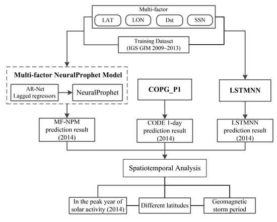
2. Materials and Methods

2.1. Multi-Factor NeuralProphet Model (MF-NPM)

NeuralProphet is a neural network based on PyTorch implementation of a time series forecasting tool and is heavily inspired by Prophet, which is the popular forecasting tool developed by Facebook. In addition, it uses standard deep learning methods for training, and local conditional variables can be introduced through autoregressive and covariable modules. NeuralProphet model retains the same basic model components as Prophet and can be configured as classical linear regression or neural network model, according to requirements. Compared with the Prophet model, NeuralProphet uses PyTorch for optimization, which speeds up the modeling process, and AR-NET is used to build the time series autocorrelation model. In addition, NeuralProphet also has the advantages of the customized loss function and the configurable nonlinear layer of the feedforward neural network [29,30]. The complete composition formula of NeuralProphet can be expressed as:
y ^ t = T ( t ) + S ( t ) + E ( t ) + F ( t ) + A ( t ) + L ( t )
where t is the time, y ^ t is the predicted value, T ( t ) is the trend information, S ( t ) is the seasonal effect, E ( t ) refers to the event and holiday effect, F ( t ) denotes the regression effect for future-known exogenous variables, A ( t ) is the auto-regression effect based on past observations, and L ( t ) is the regression effect for lagged observations of exogenous variables.
As we have previously stated, this paper used the MF-NPM based on the NeuralProphet model with AR-Net and lagged regressors. Lagged regressors were used to correlate the solar activity index, geomagnetic activity index, geographic coordinates, and IGS GIM data variables to our TEC time series database.

2.2. Long Short-Term Memory Neural Network (LSTMNN) Model

In this study, the deep learning methods for LSTMNN were built on top of TensorFlow. The LSTMNN model solves the shortcomings of recurrent neural networks in the process of backpropagation, such as gradient explosion and disappearance, and can better learn the long-term dependence of TEC on time series information. The LSTMNN neurons add the structure of three “gates” (input gate, forgetting gate, and output gate) to replace RNN neurons to improve the long-term sequence prediction [31,32]. The gate unit of the network neuron structure can be described by the following functions:
I t = σ ( w i [ h t 1 , X t ] + b i )
f t = σ ( w f [ h t 1 , X t ] + b f )
O t = σ ( w o [ h t 1 , X t ] + b o )
C t = f t C t 1 + I t t a n h ( w c [ h t 1 , X t ] + b c )
h t = t a n h ( C t ) O t
where X t is the time series of the input; h t 1 is the short-term memory of neurons; I t , f t , and O t , respectively, represent the input gate, forgetting gate, and output gate; C t 1 represents the unit state at the last moment; C t is the updated unit state; b is the bias term, w is the weight matrix; h t is the output value; σ is the sigmoid activation function; the range is (0, 1); and tanh is a hyperbolic tangent activation function that controls the state and output of the unit.

3. Data Processing and Analysis

3.1. Data and Model Parameter Settings

In this study, the input parameters of the MF-NPM and LSTMNN models include four parts: geographic coordinates, the solar activity index, the geomagnetic activity, and historical TEC data. The ionospheric TEC time series database used for modeling is the IGS GIM data from 2009–2014, obtained from CDDIS (https://cddis.nasa.gov/archive/gnss/products/ionex/, accessed on 20 September 2022), with a spatiotemporal resolution of 2.5° × 5° × 2 h. These TEC data are divided into training and test subsets during the operations of the modeling process, among which datasets for 2009–2013 are used to train the MF-NPM and LSTMNN models, and the data from 2014 are selected as the test dataset to validate the two models’ performance by sliding 1 day. The study area ranges from 70~140°E and 5~60°N, covering the whole region of China. In addition, as interplanetary influence factors affect the spatiotemporal characteristics of TEC, the equatorial ring current index Dst provided by ICSU-WDS Data Center (https://wdc.kugi.kyoto-u.ac.jp/wdc/Sec3.html, accessed on 20 September 2022) and the solar activity index SSN provided by German Geoscience Research Center GFZ (ftp://ftp.gfz-potsdam.de/pub/home/obs/, accessed on 20 September 2022) are used as input parameters, together with ionospheric TEC for participating in model construction. The levels of interplanetary influence factors are shown in Table 1, and the geomagnetic and solar activities from 2008 to 2014 are shown in Figure 1. Moreover, the relevant data refer to the Chinese Geomagnetic Violence Grade Standard Document (GB/T 31160-2014) and the NOAA Space Weather Prediction Center.
The period 2009–2014 belongs to the 24th solar cycle, and the solar activity peak was reached in April 2014. Figure 1 indicates that the SSN values showed an overall upward trend from 2009 to 2014 and reached a maximum of 220 on 27 February 2014. Therefore, this paper studies the applicability and superiority of MF-NPM in predicting ionospheric TEC in 2014, the peak year of the 24th solar activity cycle, and produces a comprehensive comparison and analysis with the LSTMNN model.
The specific parameter settings of the MF-NPM and LSTMNN model are illustrated in Table 2. The default settings are used for other relevant parameters in the MF-NPM.

3.2. Results and Discussion

In this paper, the mean bias, root mean square error (RMSE) of model residuals, relative accuracy (RA), and mean TEC (MTEC) are used as metrics to evaluate the prediction accuracy of TEC:
B i a s = 1 n i = 1 n t e c p , i t e c r , i
R M S E = 1 n i = 1 n ( t e c p , i t e c r , i ) 2
R A = 1 n i = 1 n ( 1 t e c p , i t e c r , i t e c r , i ) × 100 %
M T E C = i = 1 n ( t e c i · cos φ ) / i = 1 n cos φ
where tecp and tecr represent the TEC value of the ionospheric grid point (IGP) predicted by the models and provided by IGS, respectively. φ is the geographic latitude of IGP, and n is the length of the predicted TEC data. TEC is measured in the TEC Unit (TECU) where 1 TECU = 1016 el/m2.

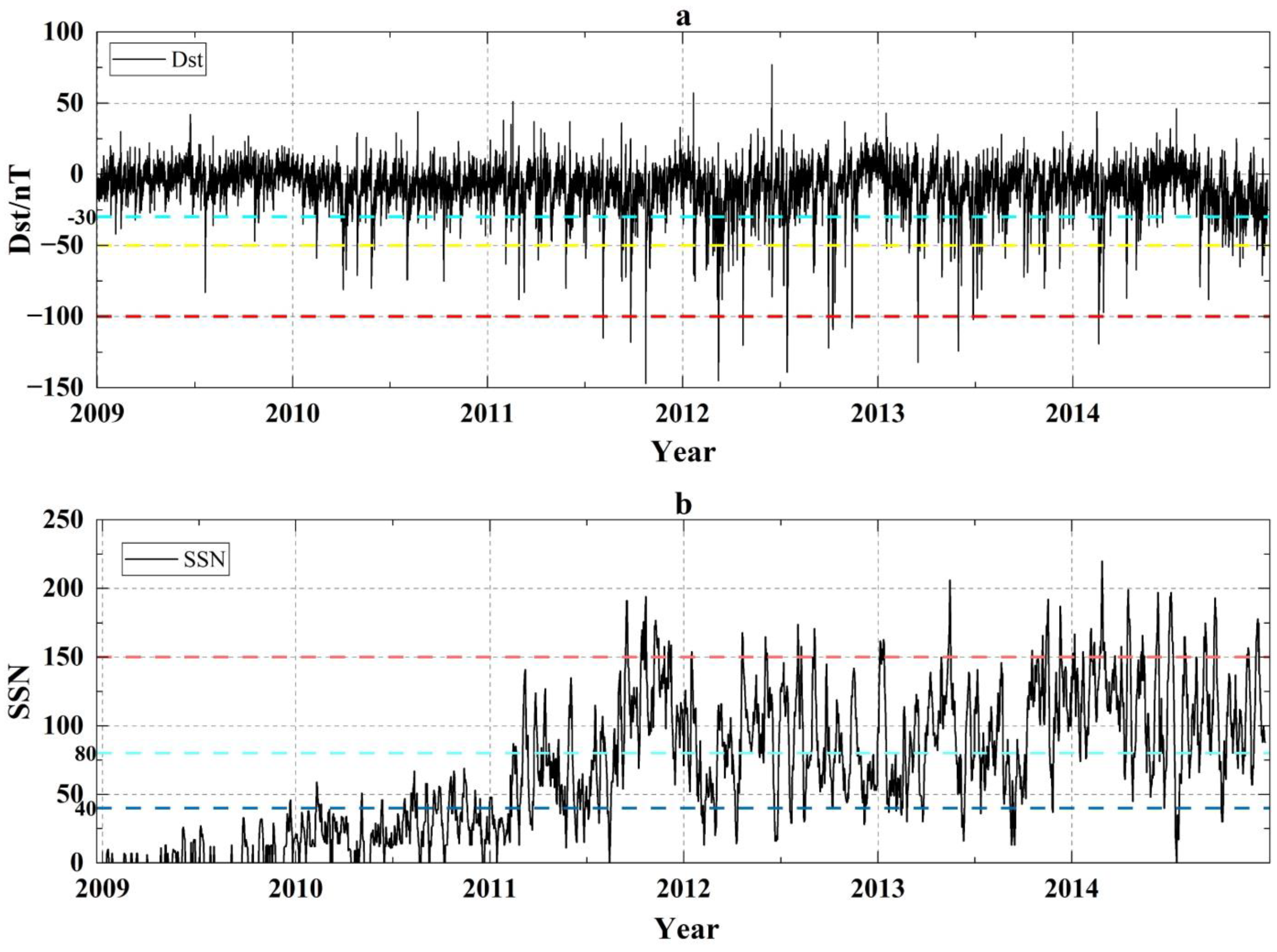
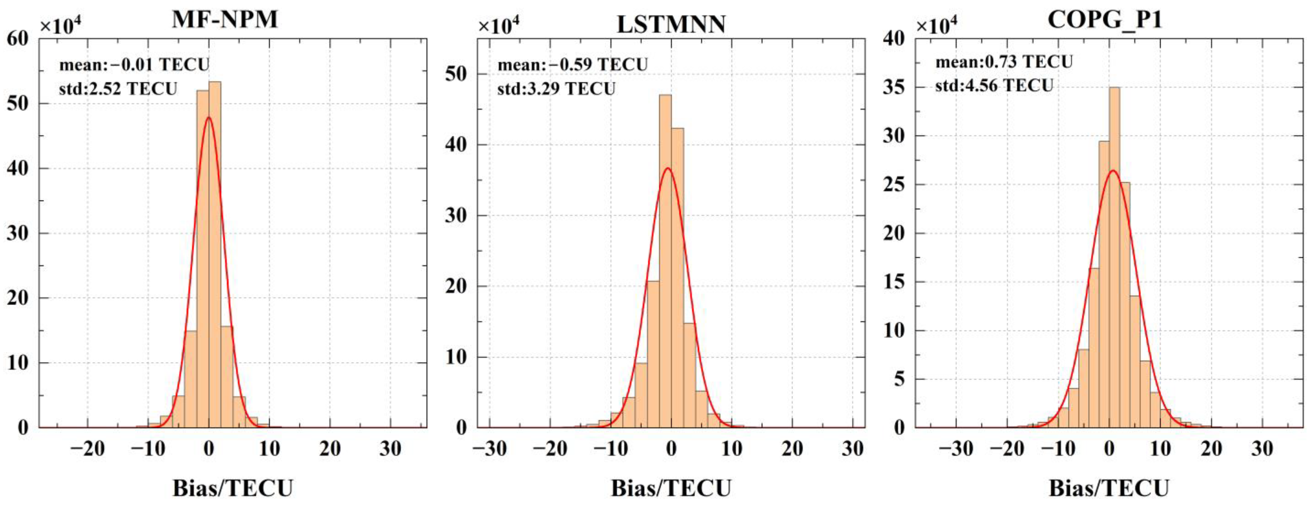
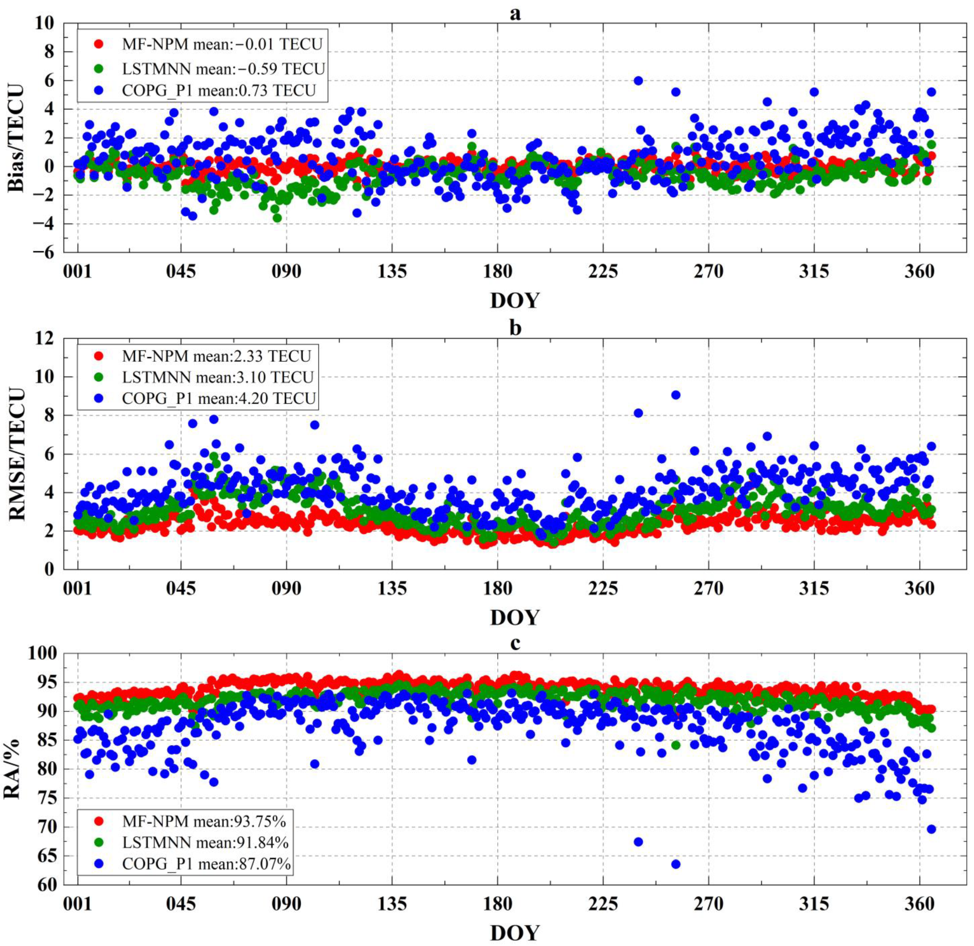
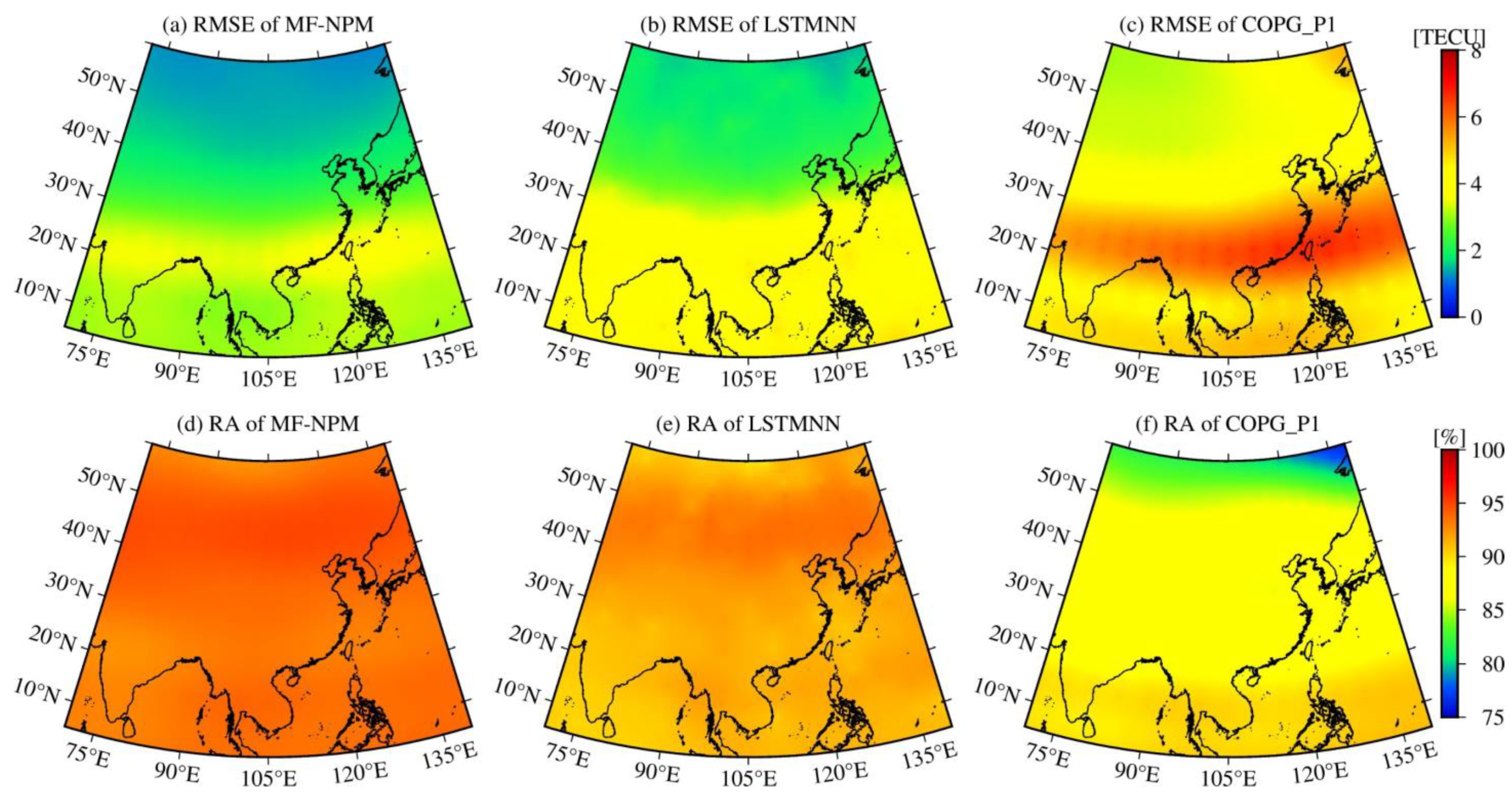
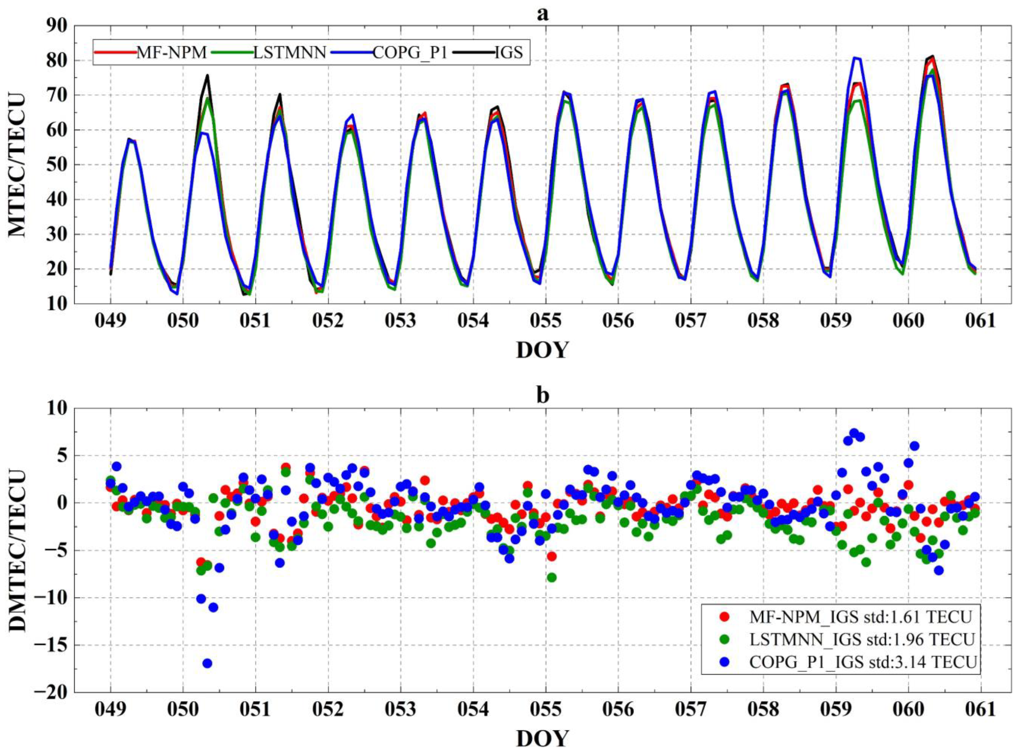
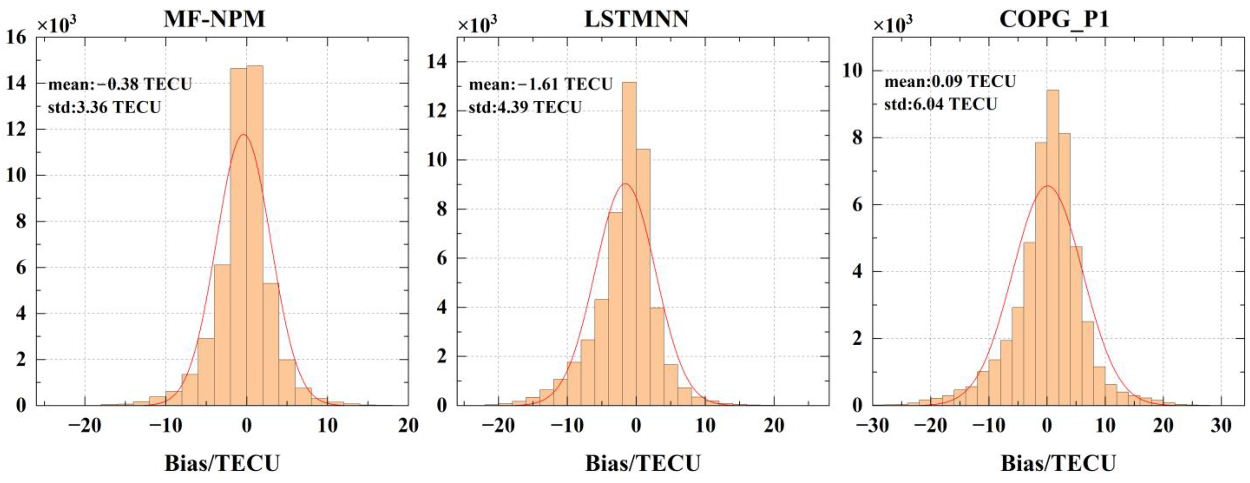
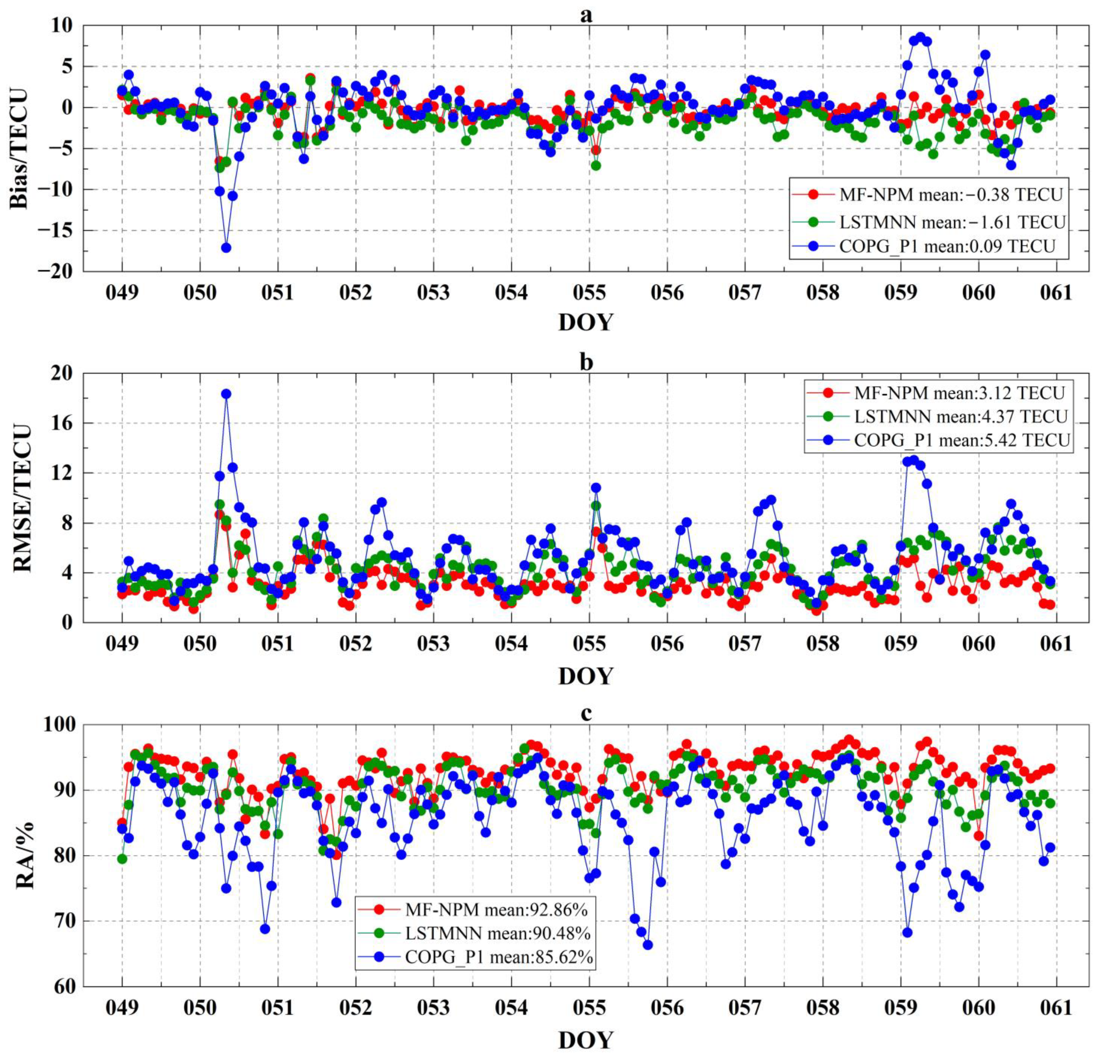
3.2.1. Prediction Accuracy Analysis in the Peak Year of Solar Activity

The overall activity level of regional ionospheric TEC can be reflected by MTEC [10]. Figure 2 shows the comparison results of the daily MTEC and the MTEC difference (DMTEC) of the MF-NPM, LSTMNN, and COPG_P1 with regard to IGS in 2014. Figure 2a illustrates that the MF-NPM, LSTMNN, and COPG_P1 can describe the detailed diurnal variations of TEC. The overall MTEC dynamics of MF-NPM, LSTMNN, and COPG are in good consistency with IGS GIMs, ranging from 19.0 to 53.5 TECU. Moreover, as shown in Figure 2b, the DMTEC distribution of MF-NPM is the most concentrated and is within 2.0 TECU, and the standard deviations of MF-NPM and LSTMNN are within 0.5 and 1.0 TECU, respectively, except that of COPG, which is up to 1.7 TECU. In conclusion, MF-NPM can better reflect the variation of ionospheric TEC in the study region.
Figure 3 shows the histogram of prediction biases of MF-NPM, LSTMNN, and COPG_P1 in the peak year of solar activity (2014), e.g., the test data set. As illustrated in the subfigures, the mean biases of MF-NPM, LSTMNN, and COPG_P1 are all within 1.0 TECU. The mean bias of MF-NPM is −0.01 TECU, which is the closest to 0 represented in the first subfigure, indicating that it is a more unbiased estimation than the latter two models. Furthermore, the standard deviation (std) of MF-NPM prediction biases is 2.52 TECU, which is 0.77 and 2.04 TECU lower than that of LSTMNN and COPG_P1, respectively. As one can see, MF-NPM shows the smallest error. The statistical bias distributions of the foresaid corresponding models are given in Table 3. The percentage of the interval [−2, 2] TECU of the MF-NPM biases accounts for 69.70%, which is 10.53% and 27.03% higher than that of LSTMNN and COPG_P1, respectively. Moreover, the percentage of interval [−5, 5] TECU for the three models biases is 94.00%, 88.46%, and 78.59%; [−10, 10] TECU is 99.50%, 98.32%, and 95.54%, [−15, 15] TECU is 99.95%, 99.77%, and 98.94%; and [−20, 20] TECU is 99.99%, 99.97%, and 99.76%. Hence, we can see that most biases are within ±10 TECU for MF-NPM. The synthesis statistic of biases suggests that MF-NPM yields a smaller error and can provide better performance than LSTMNN and COPG_P1.
Figure 4 shows the 2014 bias, RMSE, and relative accuracy averaged by a 1-day running average. As shown in Figure 4, the MF-NPM features minimal error and the errors distribution of TEC prediction results of MF-NPM are more concentrated compared with LSTMNN and COPG_P1. Furthermore, the upper Figure 4a shows the bias of MF-NPM varying from −1.33 to 1.12 TECU with an average of −0.01 TECU. Nevertheless, the bias is −3.60 to 1.53 TECU and −3.46 to 5.98 TECU for LSTMNN and COPG, respectively, with mean values of −0.59 and 0.73 TECU. Figure 4b presents the RMSE of the MF-NPM model as being 2.33 TECU, and the accuracy is 0.77 TECU and 1.87 TECU higher than that of LSTMNN and COPG_P1. As shown in Figure 4c, the average annual RA of MF-NPM is 93.75%, which is 1.91% and 6.68% higher than LSTMNN and COPG_P1, respectively. Therefore, in terms of accuracy, MF-NPM also has a good performance, and its bias, RMSE, and RA are better than LSTMNN and COPG_P1.
Table 4 lists the errors of ionospheric TEC predicted by MF-NPM, LSTMNN, and COPG_P1 in the low latitude region (5~30°N) and middle latitude region (30~60°N). The 2D spatial distributions for respective RMSE and relative accuracy of forecasted TEC values obtained from the three models with respect to IGS GIMs are illustrated in Figure 5 (top and bottom panels). It can be seen that the TEC prediction errors of MF-NPM, LSTMNN, and COPG_P1 are higher in the low latitude region than in the middle latitude region, and the main trend is that RMSE increases and the RA decreases with the increase in latitudes, combined with Table 4 and Figure 5. On the one hand, the RMSE of the MF-NPM model is 3.24 TECU, the accuracy is 1.08 and 2.05 TECU higher than LSTMNN and COPG_P1, and its RA is 93.33%, which is 2.12% and 4.2% higher than LSTMNN and COPG_P1, in the low-latitude region, respectively. On the other hand, the RMSE of the MF-NPM is 1.70 TECU, the accuracy is 0.52 and 2.20 TECU higher than LSTMNN and COPG_P1, and its RA is 94.06%, which is 1.73% and 8.59% higher than LSTMNN and COPG_P1, in the mid-latitude region, respectively.

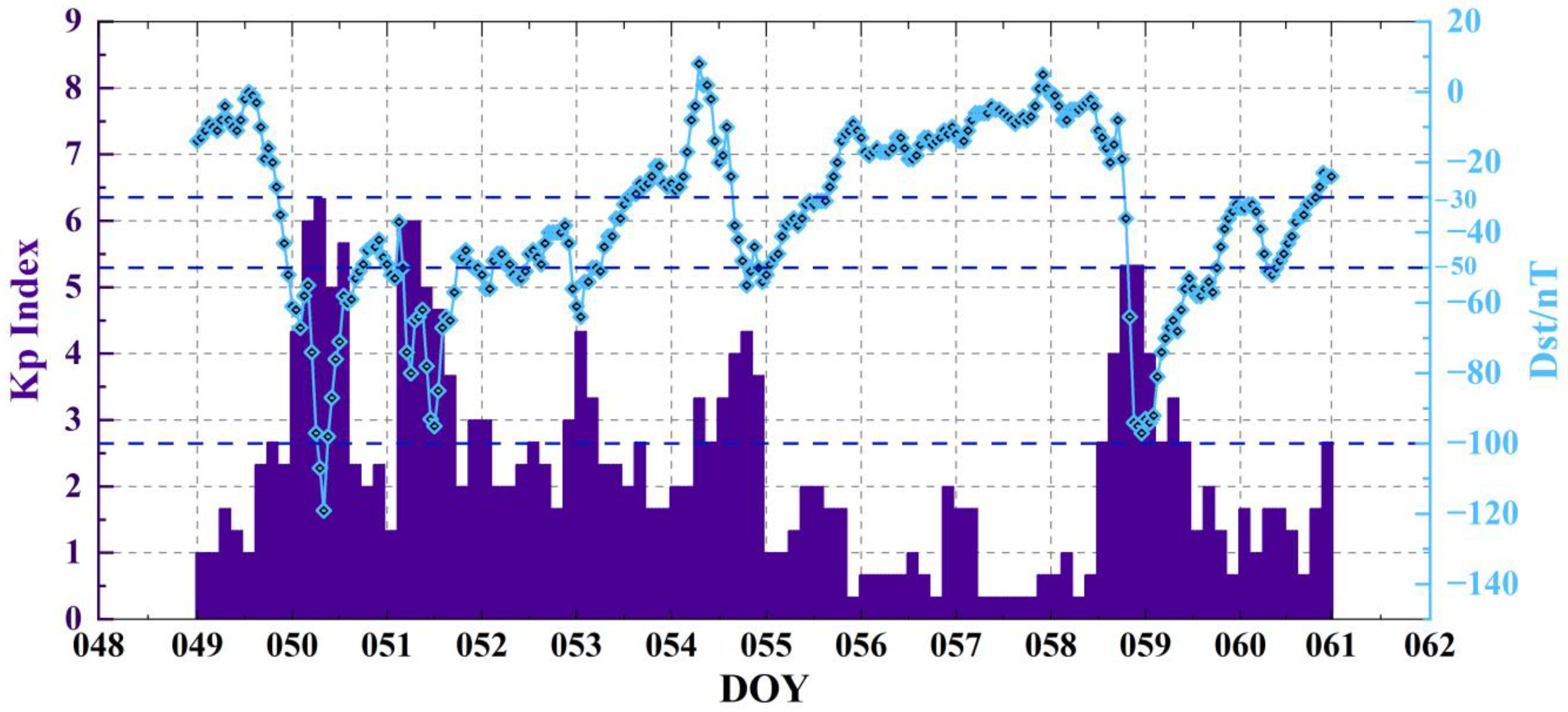
3.2.2. Accuracy Analysis during Geomagnetic Storm Period

The geomagnetic storm events that occurred during the geomagnetic storm period (DOY049~060) in the peak year of solar activity (2014) were selected to further analysis of the accuracy, reliability, and applicability of MF-NPM for predicting ionospheric TEC in the study area. The variations of geomagnetic activity in terms of Dst and Kp indices varied from DOY049 to 060 in 2014 is shown in Figure 6. During this period, the Dst varied from 7 to −112 nT and reached two obvious peak values of −112 nT (DOY050) and −99 nT (DOY059), indicating the major/strong and moderate geomagnetic storm events.
The DMTEC indicates the difference between TEC prediction and reference value (e.g., IGS GIM products). Figure 7 shows diurnal variations of MTEC and DMTEC in China from DOY049-060. It is observed from Figure 7a that the predicted TEC from the three models are following IGS-GIM patterns with overestimations and underestimations of IGS-GIM values in China. However, the overall TEC dynamics of MF-NPM, LSTMNN, and COPG_P1 are in good consistency with IGS GIMs, ranging from 12.7 to 80.7 TECU. As can be seen from the results in Figure 7b, the standard derivations of MF-NPM and LSTMNN is within 2 TECU, except that of COPG_P1, which is up to 3 TECU. In addition, two peaks reached in the variation of geomagnetic activity on DOY050 and 059 lead to an increase in the difference during the corresponding two days. As shown in Figure 7b, it can be seen that the DMTEC on the most disturbed day (DOY050) is pronounced, reaching the maximum −6.65, −7.14, and −16.93 TECU for MF-NPM, LSTMNN, and COPG_P1, respectively. The geomagnetic storms contribute to the above bias characteristics.
Moreover, the corresponding statistics of the biases predicted by MF-NPM, LSTMNN, and COPG_P1 are represented by Figure 8 and Table 5. As shown in the subfigures, the mean biases and standard derivations of TEC predicted by the selected models are −0.38, −1.61, and 0.09 TECU and 3.36, 4.39, and 6.04 TECU, respectively. Generally, an agreement is reached well across the whole area of China. The biases fulfill the Gaussian distribution well, meaning that biases comply with the random error distribution. However, the MF-NPM features minimal standard derivation, which is prominently lower by 1.03 and 2.68 TECU than LSTMNN and COPG, respectively. By contrast, the mean bias (TECCOPG—TECIGS) for COPG_P1 is negative (i.e., −0.09 TECU), which means COPG_P1 TEC was marginally smaller during the geomagnetic storm period. Conversely, the mean bias for NM-NPM and LSTMNN is positive. It is likely attributed to the influence of SSN and Dst as input parameters, which compensate for mismodelling to some extent due to the single layer model. Moreover, all standard deviations remain within 4.5 TECU during the period, except that of COPG_P1, which reaches 6.0 TECU.
Additionally, Table 5 summarizes the prediction biases from DOY049~060 in 2014. the percentage of the interval [−2, 2] for the MF-NPM biases is 59.18%, whereas that for [−5, 5] is 88.11%, [−10, 10] is 98.08%, [−15, 15] is 99.73, and [−20, 20] is 99.99%. As we can see from the statistics above, most of the biases are within ±10 TECU, which is more concentrated than the other two models. Although the above comparison results indicated that MF-NPM shows outperformance relative to LSMNN and COPG_P1, it still does not fully reflect the complex changes brought by the geomagnetic storms, with respect to IGS.
The diurnal variations of RMSE and mean relative accuracy between the TEC prediction results of the three models and IGS from DOY049~060 are shown in Figure 9. The errors of three models exhibit significant deviations with regard to IGS on DOY050 and 059, respectively. The upper Figure 9a shows the bias of MF-NPM varying from −6.65 to 3.57 TECU with an average of −0.38 TECU. Moreover, the bias is −7.37 to 3.27 TECU and −17.09 to 8.59 TECU for LSTMNN and COPG_P1, respectively, with mean values of −1.61 and 0.09 TECU. The results indicate that the mean biases of MF-NPM and COPG_P1 are 1.23 and 1.70 TECU higher than LSTMNN, respectively. According to Equations (8) and (9), the smaller RMSE and relative error would mean better prediction effects. As can be seen from the following two figures, the general trends are as expected within the results. The performance of MF-NPM is usually better than LSTMNN and COPG_P1. Figure 9b presents the RMSE of MF-NPM, varying from 0.96 to 8.67 TECU with an average of 3.12 TECU. Nevertheless, the RMSE is 1.49 to 9.50 TECU and 1.59 to 18.34 TECU for LSTMNN and COPG_P1, respectively, with mean values of 4.37 and 5.42 TECU. The results indicate that the absolute accuracy (RMSE) of MF-NPM is 1.25 and 2.30 TECU higher than LSTMNN and COPG_P1, respectively.
The variations of statistical relative accuracy for the three models with respect to IGS GIMs are displayed in the corresponding Figure 9c. The figure shows that MF-NPM, which is represented by blue points, has better relative accuracy than LSTMNN and COPG_P1. Taking a further examination of this subfigure, it is revealed that the relative accuracy of MF-NPM is 92.86%, which is consistently higher than that of LSTMNN and COPG_P1, indicating that MF-NPM has the smallest relative error. Moreover, two peaks are observed on DOY050 and 059, which corresponded to the geomagnetic activities mentioned above. Based on Figure 6, the geomagnetic activity was significantly enhanced on DOY050 and 059, and the maximum of Kp and Dst reached 6 and 112 nT and 6 and 99 nT, respectively. Therefore, the accuracy of MF-NPM is reduced, but the relative accuracy remains above 90%, and the RMSE also keeps within 10.0 TECU, as can be seen from Figure 8. The experimental results demonstrate that the proposed MF-NPM achieve better performance than the LSTMNN and COPG_P1 during geomagnetic storms period.
Table 6 shows the statistics of errors from various models with respect to IGS GIMs in a low-latitude region (5~30°N) and mid-latitude region (30~60°N) during a period of geomagnetic storms. The results of comparison with MF-NPM, LSTMNN, and COPG_P1 at different latitudes are summarized, which indicate that TEC prediction accuracy are high for low- and mid-latitude even though daily TEC value is high. In general, the prediction results in mid-latitude region are better than those in low-latitude region. As one can see in this table, MF-NPM achieves high accuracy with RMSE and relative accuracy of 4.33 and 2.34 TECU and 92.62 and 93.04% in low- and mid-latitude regions, respectively. In contrast, for LSTMNN, it is about 6.11 and 3.00 TECU and 90.02 and 90.82% and about 6.94 and 5.14 TECU and 89.07 and 82.96% for COPG_P1. Moreover, from these comparisons in low-latitude regions, it is derived that the proposed model is 2.60% and 3.55% more accurate than LSTMNN and COPG_P1 in terms of relative accuracy values, with a reduction of 1.8 and 2.6 TECU for RMSE, respectively. Similarly, in a mid-latitude region, the accuracy of MF-NPM is 2.22% and 10.08% higher than LSTMNN and COPG_P1, and RMSE is reduced by 0.7 and 2.8 TECU, respectively.
The spatial distributions for respective RMSE and relative accuracy of forecasted TEC values obtained from the three models, with respect to IGS GIMs are illustrated in Figure 10 (top and bottom panels). It is observed from the top panel of this figure that the maximal error occurs in the low-latitude region for all the models. This is an expected result because it is in the anomaly region with maximal TEC and prominent TEC daily variability, which will lead to a larger difference in TEC values from different models. Moreover, COPG_P1 shows a high error in the low-latitude region, with the error values ranging between 7~9 TECU. Moreover, we note the obvious increases in local errors neighboring 20~35°N, with the error values ranging between 5~7 TECU and 7~9 TECU for LSTMNN and COPG_P1, but there are no such increments from MF-NPM. As shown in the bottom panel, the relative accuracy of MF-NPM varies between 92~97%, which is significantly higher than the other two models. Hence, the proposed technique of MF-NPM obtain a better accuracy and has better performance in low- and mid-latitudes during geomagnetic storm days.

4. Discussion

In this paper, a novel multi-factor regional ionospheric TEC prediction model, MF-NPM, has been constructed taking into account the solar activity index, geomagnetic activity index, and geographic coordinates. The forecasting performance of MF-NPM, trained using the dataset from 2009 to 2013, was evaluated using the test dataset (2014) by sliding 1 day. Furthermore, MF-NPM was validated with the LSTMNN model and CODE from the spatiotemporal perspective during the peak year of solar activity (2014) and geomagnetic storm. With respect to the IGS GIM, results showed that the accuracy of forecasting TEC can be improved by the MF-NPM based on AR-NET and lagged regressors significantly, in terms of bias, RMSE, and relative accuracy.
In terms of temporal perspective, the MF-NPM outperformed CODE’s and LSTMNN models in 2014 and its geomagnetic storms. In the peak year of solar activity (2014), the variations of TEC predicted by MF-NPM are more consistent with IGS GIM, compared with COPG_P1 and LSTMNN. The biases of the foresaid corresponding models are −0.01, −0.59, and 0.73 TECU, with the distribution within ±10 TECU accounting for 95%. Moreover, MF-NPM achieves the best performance with RMSE and RA of 2.33 TECU and 93.75%, which are much smaller than 3.10 and 4.20 TECU and 91.84 and 87.07% of LSTMNN and COPG_P1, respectively. Additionally, during geomagnetic storms, although the accuracy of MF-NPM, LSTMNN, and COPG_P1 are all reduced to some extent due to the influence of geomagnetic disturbances on the ionosphere, the performance of MF-NPM is still better than that of LSTMNN and COPG_P1 and exhibits significant deviations with regard to IGS on DOY050 and 059. The mean biases are −0.38, −1.61, and 0.09 TECU, respectively, and most biases are within ±10 TECU with the percentage above 90%. Results suggest that RMSE and RA of MF-NPM are 3.12 TECU and 92.86% which are lower than 4.37 and 5.42 TECU and 90.48 and 85.62% of LSTMNN and COPG_P1, respectively.
From the spatial perspective, MF-NPM and LSTMNN models outperform CODE in low–middle latitudes with MF-NPM being the best. The main reason that the maximal error occurs in the low-latitude region for all the models is because the anomaly region with maximal TEC and prominent TEC daily variability will lead to a larger differential in TEC values from different models. In 2014, the RMSE and RA of MF-NPM are 3.24 TECU and 93.33%, which are better than LSTMNN (4.32 TECU, 91.21%) and COPG_P1 (5.29 TECU, 89.13%) in the low latitudes, respectively. In addition, MF-NPM also provide better performance than LSTMNN and COPG_P1 in the mid-latitude region, with respect to the RMSE and RA, which are improved by 0.52 and 2.20 TECU and 1.73 and 8.59%, respectively. Additionally, equatorial ionospheric anomaly (EIA) and electron density anomaly are enhanced by geomagnetic storms. During geomagnetic storms, the RMSE and RA of MF-NPM are 4.33 TECU and 92.62%. In addition, the accuracy of mid latitudes is also higher than that of low latitudes with improved accuracy of the average RMSE and RA of 0.70 and 2.80 TECU and 2.22 and 10.08%, respectively.
In general, the new model, MF-NPM, can capture the variations of ionospheric TEC in the high solar activity year and geomagnetic storms period. Moreover, the prediction effects of MF-NPM are the best whether they are from a time or spatial perspective. It is noted that the ionospheric TEC time series database used for the training model is the GIM data covering China from 2009–2014. Therefore, future work will be focused on constructing a global TEC prediction model using GNSS real-time or measurement data and further optimizing and improving the model.

5. Conclusions

According to the analyzed results, it is recommended that MF-NPM would provide a better accuracy level for the ionospheric correction in the regional area over China and its neighborhood to improve the correction effect of ionospheric delay in the high solar activity year and during the geomagnetic storm period.

Author Contributions

Conceptualization, H.W., L.H. (Ling Huang) and Y.L.; Methodology, H.W., L.H. (Ling Huang), Y.L. and H.Z.; Formal analysis, H.W. and L.H. (Ling Huang); Validation, L.H. (Ling Huang), H.W., L.H. (Liangke Huang) and L.L.; Writing—original draft preparation, H.W. and L.H. (Ling Huang); Writing—review and editing, L.H. (Ling Huang), H.W., Y.L., H.Z., L.L. and L.H. (Liangke Huang). All authors have read and agreed to the published version of the manuscript.

Funding

This research was funded by the Guangxi Science and Technology Base and Talent Project (Grant No. Guike AD19245060), the Guangxi Natural Science Foundation of China (Grant No. 2020GXNSFBA159033), the Guangxi Key Laboratory of Spatial Information and Geomatics (Grant No. 19-050-11-24), and the National Natural Science Foundation of China (Grant No. 42064002).

Institutional Review Board Statement

Not applicable.

Informed Consent Statement

Not applicable.

Data Availability Statement

The International GNSS Service (IGS) GIM data and the one-day forecast data from Center for Orbit Determination in Europe (CODE) used in our study can be accessed from Crustal Dynamics Data Information System (CDDIS) (https://cddis.nasa.gov/gnss/products/ionex/, accessed on 20 September 2022). The geomagnetic activity index Kp data and the solar activity index (F10.7 and SSN) data were downloaded from the GFZ (https://www.gfz-potsdam.de/en/kp-index/, accessed on 20 September 2022). The geomagnetic activity index Dst data were downloaded from the World Data Center for Geomagnetism, Kyoto (https://wdc.kugi.kyoto-u.ac.jp/wdc/Sec3.html, accessed on 20 September 2022).

Acknowledgments

The authors would like to thank the IGS CDDIS, CODE, GFZ, and WDCG for providing the relevant data.

Conflicts of Interest

The authors declare no conflict of interest. The funders had no role in the design of the study; in the collection, analyses, or interpretation of data; in the writing of the manuscript; or in the decision to publish the results.

References

  1. Bilitza, D.; Pezzopane, M.; Truhlik, V.; Altadill, D.; Reinisch, B.W.; Pignalberi, A. The International Reference Ionosphere Model: A Review and Description of an Ionospheric Benchmark. Rev. Geophys. 2022, 60, e2022RG000792. [Google Scholar] [CrossRef]
  2. Klobuchar, J.A. Ionospheric Time-Delay Algorithm for Single-Frequency GPS Users. IEEE Trans. Aerosp. Electron. Syst. 1987, AES-23, 325–331. [Google Scholar] [CrossRef]
  3. Bent, R.B.; Llewellyn, S.K.; Nesterczuk, G.; Schmid, P. The development of a highly-successful worldwide empirical ionospheric model and its use in certain aspects of space communications and worldwide total electron content investigations. In Effect of the Ionosphere on Space Systems and Communications; National Technical Information Service: Springfield, VA, USA, 1975; pp. 13–28. [Google Scholar]
  4. Nava, B.; Coïsson, P.; Radicella, S.M. A new version of the NeQuick ionosphere electron density model. J. Atmos. Sol. Terr. Phys. 2008, 70, 1856–1862. [Google Scholar] [CrossRef]
  5. Abhigna, M.; Sridhar, M.; Harsha, P.; Krishna, K.S.; Ratnam, D.V. Broadcast ionospheric delay correction algorithm using reduced order adjusted spherical harmonics function for single-frequency GNSS receivers. Acta Geophys. 2021, 69, 335–351. [Google Scholar] [CrossRef]
  6. Georgiadiou, Y. Modeling the Ionosphere for an Active Control Network of GPS Stations; LGR Series; Delft Geodetic Computing Centre: Delft, The Netherlands, 1994. [Google Scholar]
  7. Han, D.; Yun, H.; Kee, C. Performance evaluation of ionosphere modeling using spherical harmonics in the Korean Peninsula. J. Position. Navig. Timing 2013, 2, 59–65. [Google Scholar] [CrossRef] [Green Version]
  8. Li, Z.; Wang, N.; Wang, L.; Liu, A.; Yuan, H.; Zhang, K. Regional ionospheric TEC modeling based on a two-layer spherical harmonic approximation for real-time single-frequency PPP. J. Geod. 2019, 93, 1659–1671. [Google Scholar] [CrossRef]
  9. Mehmood, M.; Saleem, S.; Filjar, R.; Naqvi, N.A.; Ahmed, A. Total Electron Content (TEC) estimation over Pakistan from local GPS network using spherical harmonics. Ann. Geophys. 2021, 64, GD102. [Google Scholar] [CrossRef]
  10. Schaer, S. Mapping and predicting the Earth’s ionosphere using the Global Positioning System. Ph.D. Thesis, University of Bern, Bern, Switzerland, 1999. [Google Scholar]
  11. Dabbakuti, J.R.K.K.; Peesapati, R.; Panda, S.K.; Thummala, S. Modeling and analysis of ionospheric TEC variability from GPS–TEC measurements using SSA model during 24th solar cycle. Acta Astronaut. 2021, 178, 24–35. [Google Scholar] [CrossRef]
  12. Sivavaraprasad, G.; Venkata Ratnam, D. Performance evaluation of ionospheric time delay forecasting models using GPS observations at a low-latitude station. Adv. Space Res. 2017, 60, 475–490. [Google Scholar] [CrossRef]
  13. Ratnam, D.V.; Otsuka, Y.; Sivavaraprasad, G.; Dabbakuti, J.R.K.K. Development of multivariate ionospheric TEC forecasting algorithm using linear time series model and ARMA over low-latitude GNSS station. Adv. Space Res. 2019, 63, 2848–2856. [Google Scholar] [CrossRef]
  14. Hernández-Pajares, M.; Juan, J.M.; Sanz, J. Neural network modeling of the ionospheric electron content at global scale using GPS data. Radio Sci. 1997, 32, 1081–1089. [Google Scholar] [CrossRef] [Green Version]
  15. Cander, L.R. Spatial correlation of foF2 and vTEC under quiet and disturbed ionospheric conditions: A case study. Acta Geophys. 2007, 55, 410–423. [Google Scholar] [CrossRef]
  16. Habarulema, J.B.; McKinnell, L.-A.; Opperman, B.D. TEC measurements and modelling over Southern Africa during magnetic storms; a comparative analysis. J. Atmos. Sol. Terr. Phys. 2010, 72, 509–520. [Google Scholar] [CrossRef]
  17. Liu, Y.; Wang, J.; Yang, C.; Zheng, Y.; Fu, H. A Machine Learning-Based Method for Modeling TEC Regional Temporal-Spatial Map. Remote Sens. 2022, 14, 5579. [Google Scholar] [CrossRef]
  18. Huang, Z.; Yuan, H. Ionospheric single-station TEC short-term forecast using RBF neural network. Radio Sci. 2014, 49, 283–292. [Google Scholar] [CrossRef]
  19. Ghaffari Razin, M.R.; Voosoghi, B. Wavelet neural networks using particle swarm optimization training in modeling regional ionospheric total electron content. J. Atmos. Sol. Terr. Phys. 2016, 149, 21–30. [Google Scholar] [CrossRef]
  20. Ghaffari-Razin, S.R.; Moradi, A.R.; Hooshangi, N. Modeling and forecasting of ionosphere TEC using least squares SVM in central Europe. Adv. Space Res. 2022, 70, 2035–2046. [Google Scholar] [CrossRef]
  21. Iluore, K.; Lu, J. Long Short-Term Memory and Gated Recurrent Neural Networks to Predict the Ionospheric Vertical total electron Content. Adv. Space Res. 2022, 70, 652–665. [Google Scholar] [CrossRef]
  22. Shi, S.; Zhang, K.; Wu, S.; Shi, J.; Hu, A.; Wu, H.; Li, Y. An Investigation of Ionospheric TEC Prediction Maps Over China Using Bidirectional Long Short-Term Memory Method. Space Weather 2022, 20, e2022SW003103. [Google Scholar] [CrossRef]
  23. Xiong, P.; Zhai, D.; Long, C.; Zhou, H.; Zhang, X.; Shen, X. Long Short-Term Memory Neural Network for Ionospheric Total Electron Content Forecasting Over China. Space Weather 2021, 19, e2020SW002706. [Google Scholar] [CrossRef]
  24. Srivani, I.; Prasad, G.S.V.; Ratnam, D.V. A Deep Learning-Based Approach to Forecast Ionospheric Delays for GPS Signals. IEEE Geosci. Remote Sens. Lett. 2019, 16, 1180–1184. [Google Scholar] [CrossRef]
  25. Lin, X.; Wang, H.; Zhang, Q.; Yao, C.; Chen, C.; Cheng, L.; Li, Z. A Spatiotemporal Network Model for Global Ionospheric TEC Forecasting. Remote Sens. 2022, 14, 1717. [Google Scholar] [CrossRef]
  26. Bi, C.; Ren, P.; Yin, T.; Xiang, Z.; Zhang, Y. Modeling and Forecasting Ionospheric foF2 Variation in the Low Latitude Region during Low and High Solar Activity Years. Remote Sens. 2022, 14, 5418. [Google Scholar] [CrossRef]
  27. Benoit, A.G.; Petry, A. Evaluation of F10.7, Sunspot Number and Photon Flux Data for Ionosphere TEC Modeling and Prediction Using Machine Learning Techniques. Atmosphere 2021, 12, 1202. [Google Scholar] [CrossRef]
  28. Saqib, M.; Şentürk, E.; Sahu, S.A.; Adil, M.A. Comparisons of autoregressive integrated moving average (ARIMA) and long short term memory (LSTM) network models for ionospheric anomalies detection: A study on Haiti (Mw = 7.0) earthquake. Acta Geod. Et Geophys. 2022, 57, 195–213. [Google Scholar] [CrossRef]
  29. Triebe, O.; Hewamalage, H.; Pilyugina, P.; Laptev, N.; Bergmeir, C.; Rajagopal, R. NeuralProphet: Explainable Forecasting at Scale. arXiv 2021, arXiv:2111.15397. [Google Scholar]
  30. ChikkaKrishna, N.K.; Rachakonda, P.; Tallam, T. Short-Term Traffic Prediction Using Fb-PROPHET and Neural-PROPHET. In Proceedings of the 2022 IEEE Delhi Section Conference (DELCON), New Delhi, India, 11–13 February 2022; pp. 1–4. [Google Scholar]
  31. Zhang, Y.; Hou, J.; Huang, C. Integration of Satellite-Derived and Ground-Based Soil Moisture Observations for a Precipitation Product over the Upper Heihe River Basin, China. Remote Sens. 2022, 14, 5355. [Google Scholar] [CrossRef]
  32. Hochreiter, S.; Schmidhuber, J. Long short-term memory. Neural Comput. 1997, 9, 1735–1780. [Google Scholar] [CrossRef]
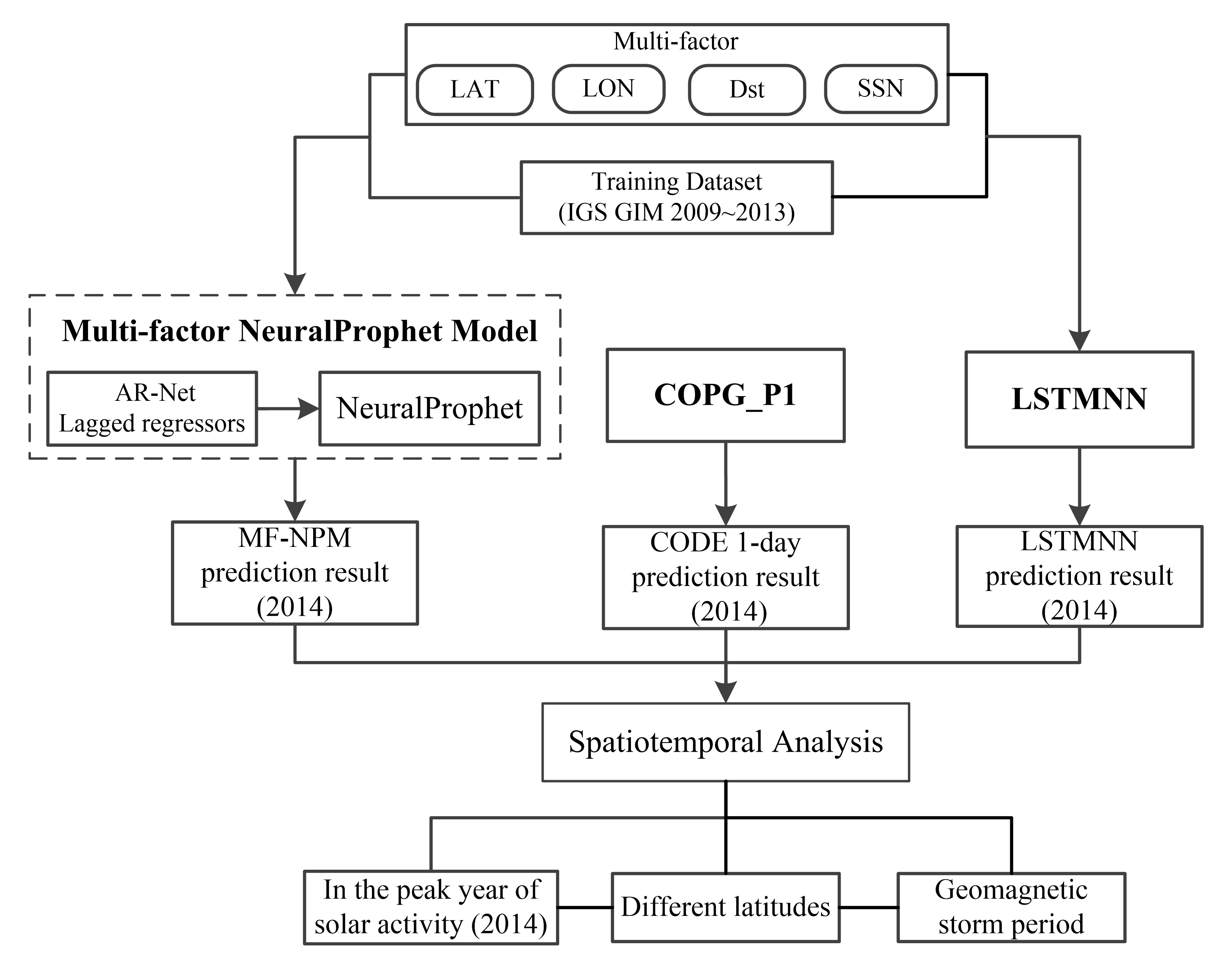
Figure 1. (a) Geomagnetic index and (b) solar activity index from 2009 to 2014. (In Figure 1a, colored dashed lines (−30, −50, and −100 nT) represent the boundary between Weak, Moderate, and Intense magnetic storms, respectively. In Figure 1b, colored dashed lines (40, 80, and 150) represent the boundary between Low, Moderate, and High solar activity, respectively.)
Remotesensing 15 00195 g001
Figure 2. The variations of daily average (a) MTEC and (b) DMTEC predicted by MF-NPM, LSTMNN, and COPG_P1 relative to IGS in the peak year of solar activity (2014).
Remotesensing 15 00195 g002
Figure 3. Histogram for MF-NPM, LSTMNN, and COPG_P1 with reference to IGS GIM in the peak year of solar activity (2014).
Remotesensing 15 00195 g003
Figure 4. The variations of (a) bias, (b) RMSE, and (c) mean relative error of MF-NPM, LSTMNN, and COPG_P1 respected to IGS in the peak year of solar activity (2014).
Remotesensing 15 00195 g004
Figure 5. The 2D spatial distributions of (ac) RMSE and (df) relative accuracy for MF-NPM, LSTMNN, and COPG in the peak year of solar activity (2014).
Remotesensing 15 00195 g005
Figure 6. Geomagnetic activity during the geomagnetic storm period (DOY049~060). (Blue dashed lines (−30, −50, and −100 nT) represent the boundary between weak, moderate, and intense magnetic storms, respectively.)
Remotesensing 15 00195 g006
Figure 7. The variations of (a) MTEC and (b) DMTEC relative to IGS during geomagnetic storms period.
Remotesensing 15 00195 g007
Figure 8. Histograms for MF-NPM, LSTMNN, and COPG_P1 with reference to IGS GIM during geomagnetic storms period.
Remotesensing 15 00195 g008
Figure 9. The variations of (a) bias, (b) RMSE, and (c) relative accuracy of MF-NPM, LSTMNN, and COPG_P1, with respect to IGS during geomagnetic storms (DOY 049~060 in 2014).
Remotesensing 15 00195 g009
Figure 10. The 2D spatial distributions of (ac) RMSE and (df) relative accuracy for MF-NPM, LSTMNN, and COPG_P1 during geomagnetic storms.
Remotesensing 15 00195 g010
Table 1. Classification of geomagnetic activity and solar activity.
Dst/nTGeomagnetic ActivitySSNSolar Activity
−30 < DstQuiet0 ≤ SSN < 40Low
−50 < Dst ≤ −30Minor Storm40 ≤ SSN < 80Moderate
−100 <Dst ≤ −50Moderate storm80 ≤ SSN < 150High
−200 < Dst ≤ −100Major Storm150 ≤ SSN < 250Very High
Dst ≤ −200Severe Storm250 ≤ SSNExtreme
Table 2. Specific parameter settings of MF-NPM and LSTMNN model.
ModelParametersSetting
MF-NPMweekly_seasonalityFALSE
yearly_seasonalityFALSE
daily_seasonalityFALSE
n_lags12
num_hidden_layers48
d_hidden4
batch_size512
epochs120
loss_funcmean_squared_error
normalize“standardize”
seasonality_mode“multiplicative”
LSTMNNLSTM layerUnits = 256, activation = ‘relu’, return_sequences = True
Dropout0.2
LSTM layer 1Units = 256, activation = ‘relu’,
return_sequences = True
Dropout10.2
LSTM layer 2Units = 256
Dense1
CompileOptimizer = ‘adam’,
Loss = ‘mean_squared_error’
batch_size512
seq_len12
epochs120
Table 3. Percentage of bias for MF-NPM, LSTMNN, and COPG_P1 in the peak year of solar activity (2014).
ModelPercentage of Bias Δ/TECU
|Δ| ≤ 2|Δ| ≤ 5|Δ| ≤ 10|Δ| ≤ 1520 < |Δ|
MF-NPM69.70%94.00%99.50%99.95%0.01%
LSTMNN59.17%88.46%98.32%99.77%0.03%
COPG_P142.67%78.59%95.54%98.94%0.24%
Table 4. RMSE and relative accuracy of the model outcomes (MF-NPM, LSTMNN, and COPG_P1) from IGS GIMs in different latitude regions during the peak year of solar activity (2014).
ModelRegionEvaluation Indicators
RMSE/TECURA/%
MF-NPMlow3.2493.33
mid1.7094.06
LSTMNNlow4.3291.21
mid2.2292.33
COPG_P1low5.2989.13
mid3.9085.47
Table 5. Percentage of bias distributions of MF-NPM, LSTMNN, and COPG_P1.
ModelPercentage of Bias Δ/TECU
|Δ| ≤ 2|Δ| ≤ 5|Δ| ≤ 10|Δ| ≤ 1520 < |Δ|
MF-NPM59.18%88.11%98.08%99.73%0.01%
LSTMNN47.53%78.30%94.51%98.98%0.12%
COPG_P134.77%69.61%90.41%96.53%0.98%
Table 6. RMSE and relative accuracy of the model outcomes (MF-NPM, LSTMNN, and COPG_P1) from IGS GIMs in different latitudes during geomagnetic storms.
ModelRegionEvaluation Indicators
RMSE/TECURA/%
MF-NPMlow4.3392.62
mid2.3493.04
LSTMNNlow6.1190.02
mid3.0090.82
COPG_P1low6.9489.07
mid5.1482.96
Disclaimer/Publisher’s Note: The statements, opinions and data contained in all publications are solely those of the individual author(s) and contributor(s) and not of MDPI and/or the editor(s). MDPI and/or the editor(s) disclaim responsibility for any injury to people or property resulting from any ideas, methods, instructions or products referred to in the content.

