
An Improved Parameter Estimation Method for High-Efficiency Multi-GNSS-Integrated Orbit Determination

Abstract
:
1. Introduction
2. GNSS Precise Orbit Determination
2.1. GNSS Observation Model
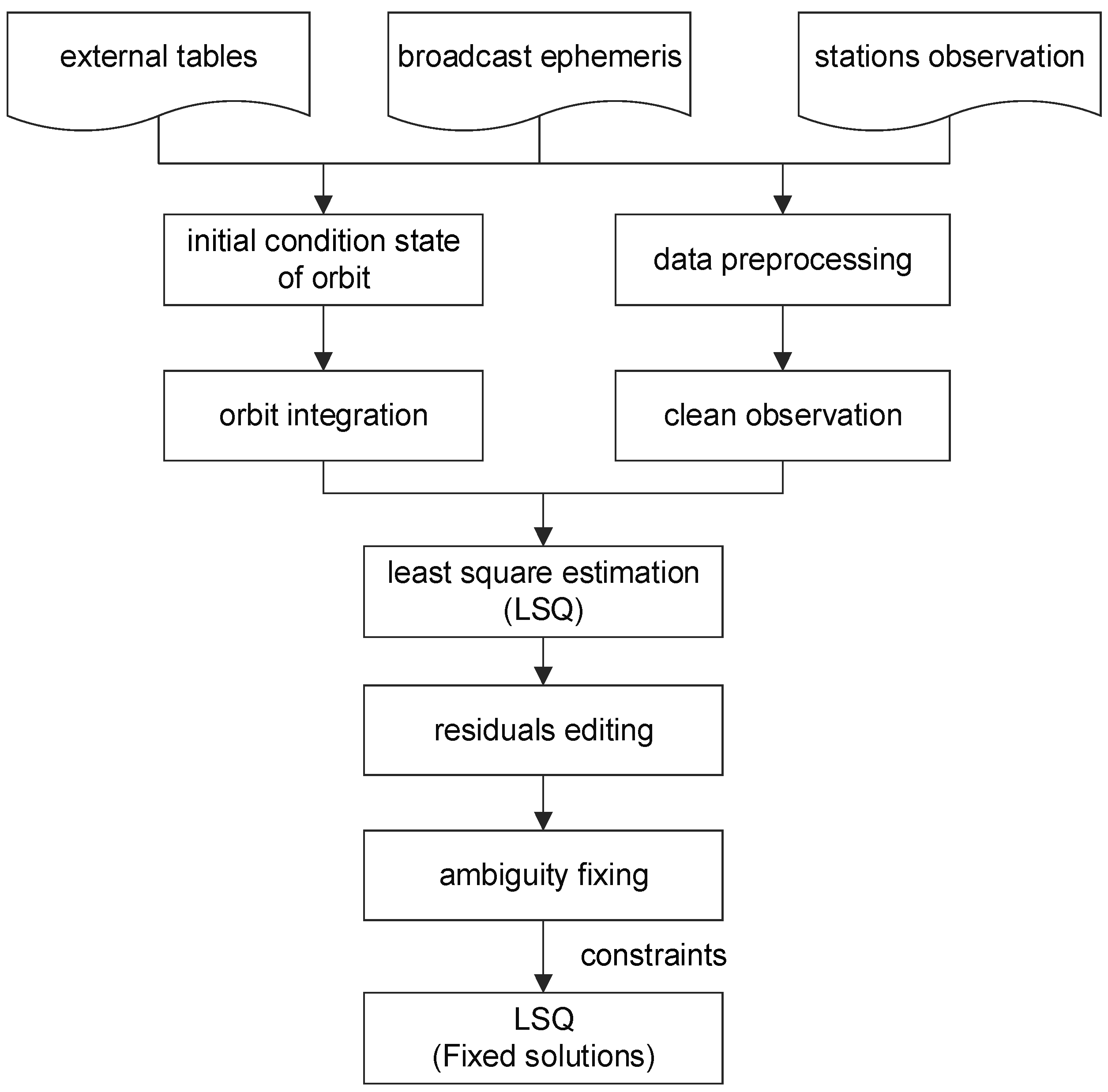
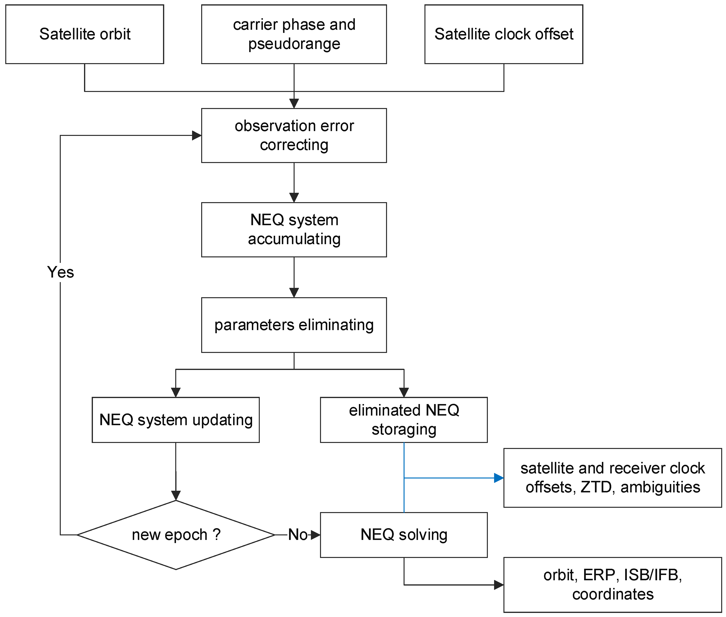
2.2. Main Processes of POD
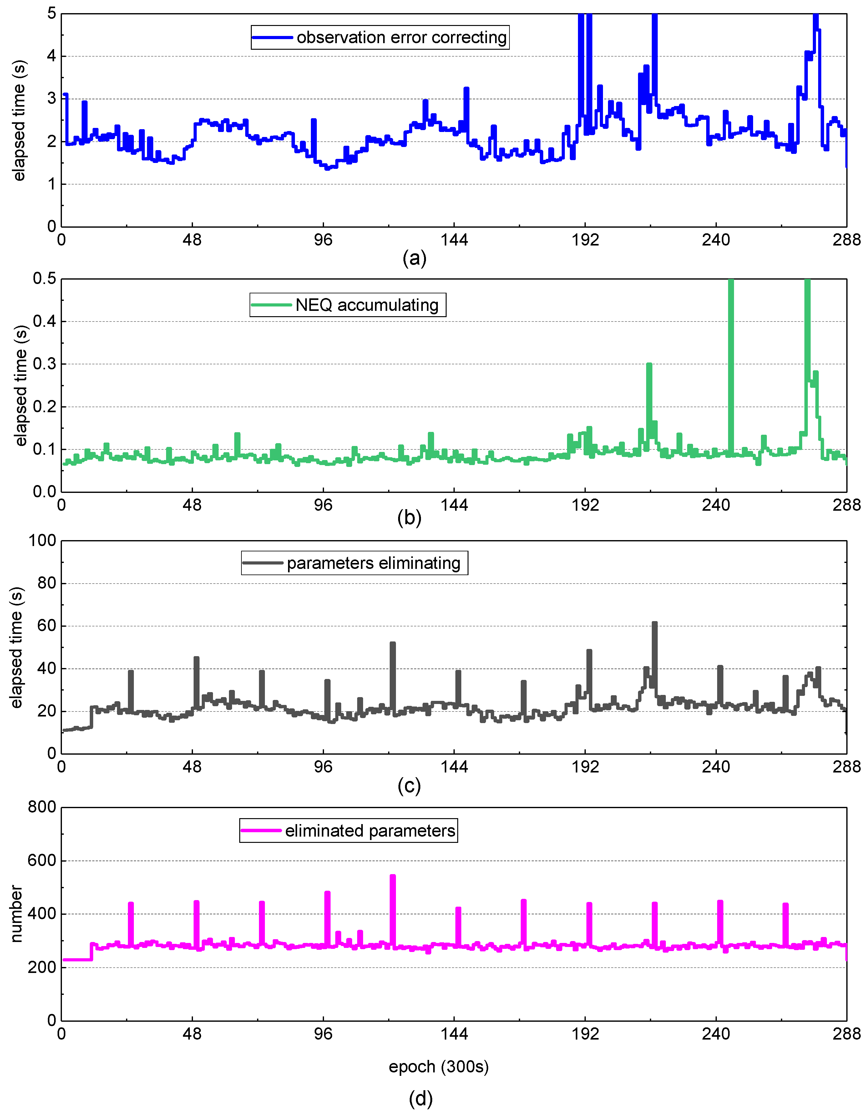
2.3. Elapsed Time Decomposition in LSQ
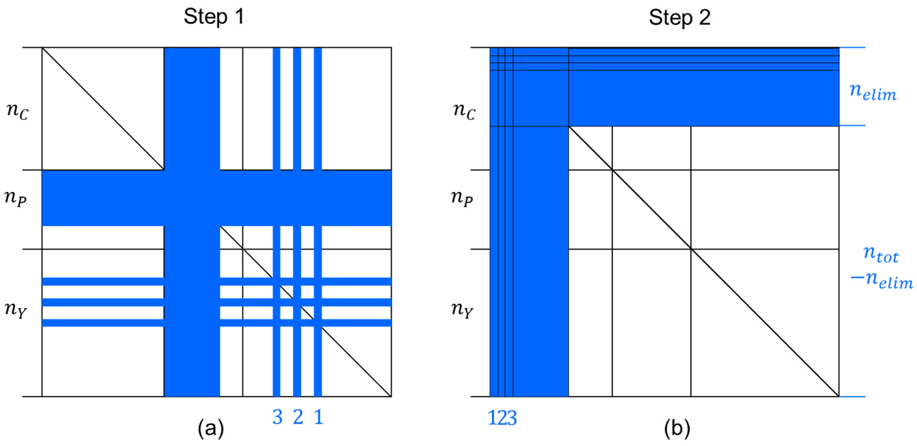
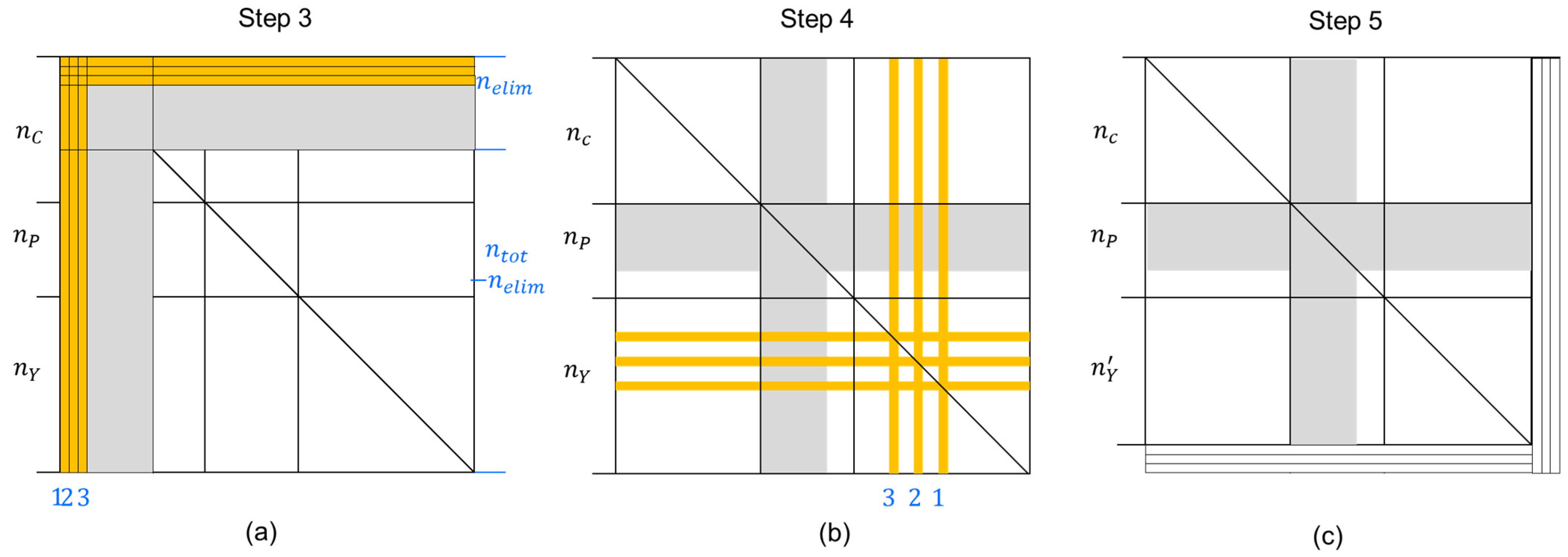
3. Improved Parameter Estimation Method
4. Experiment with the Multi-GNSS-Integrated POD
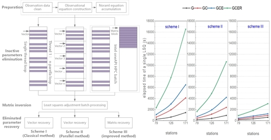
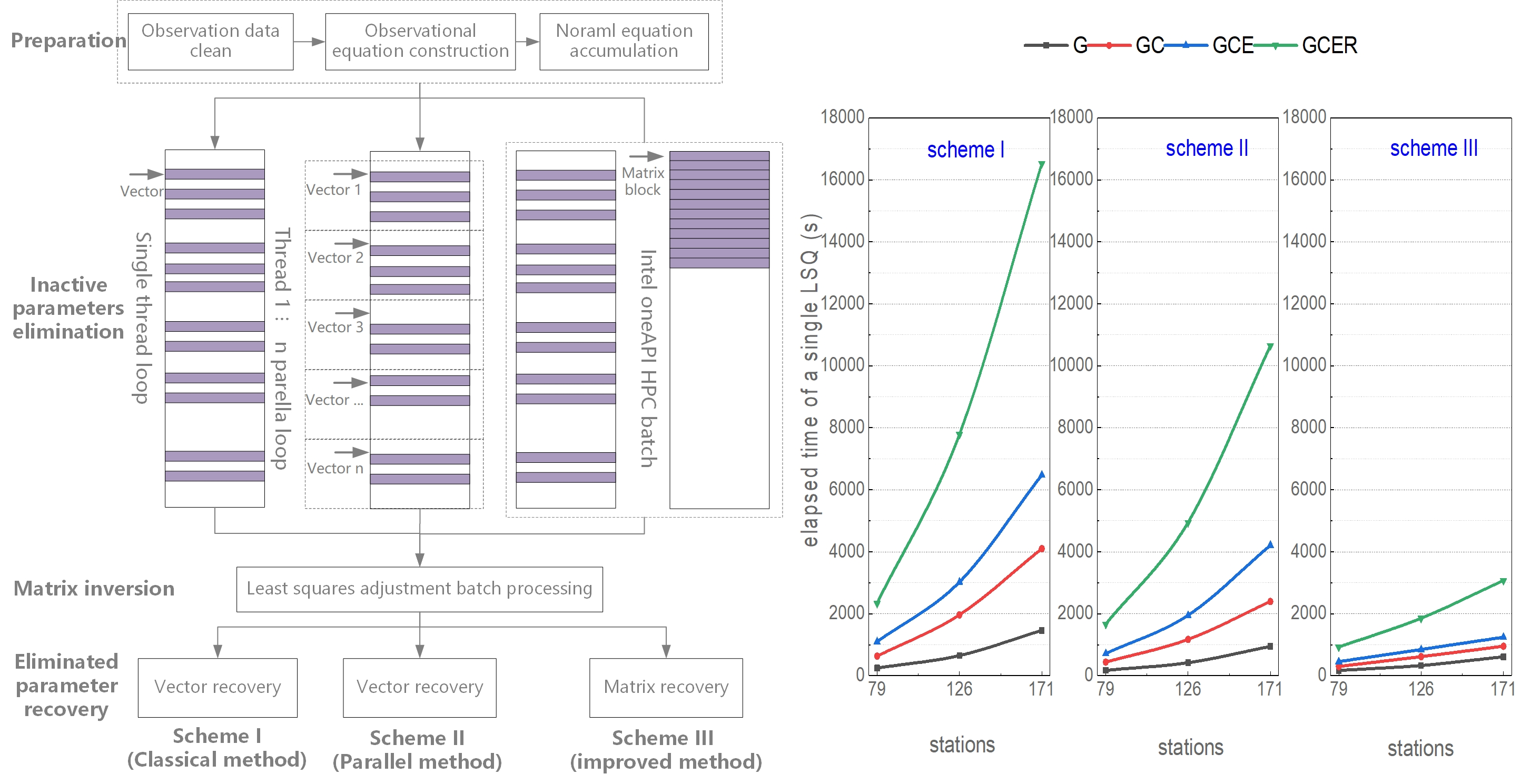
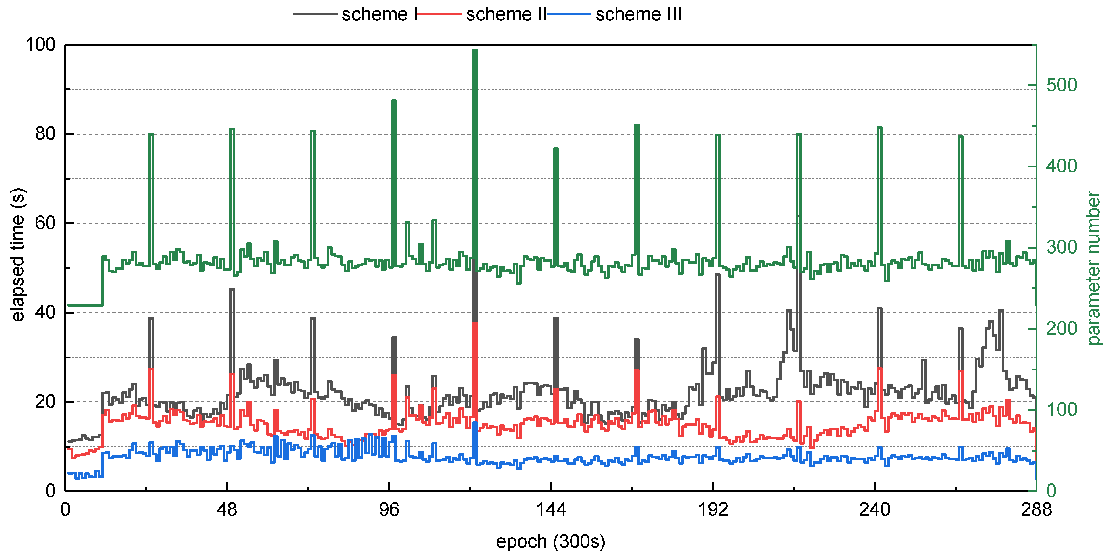
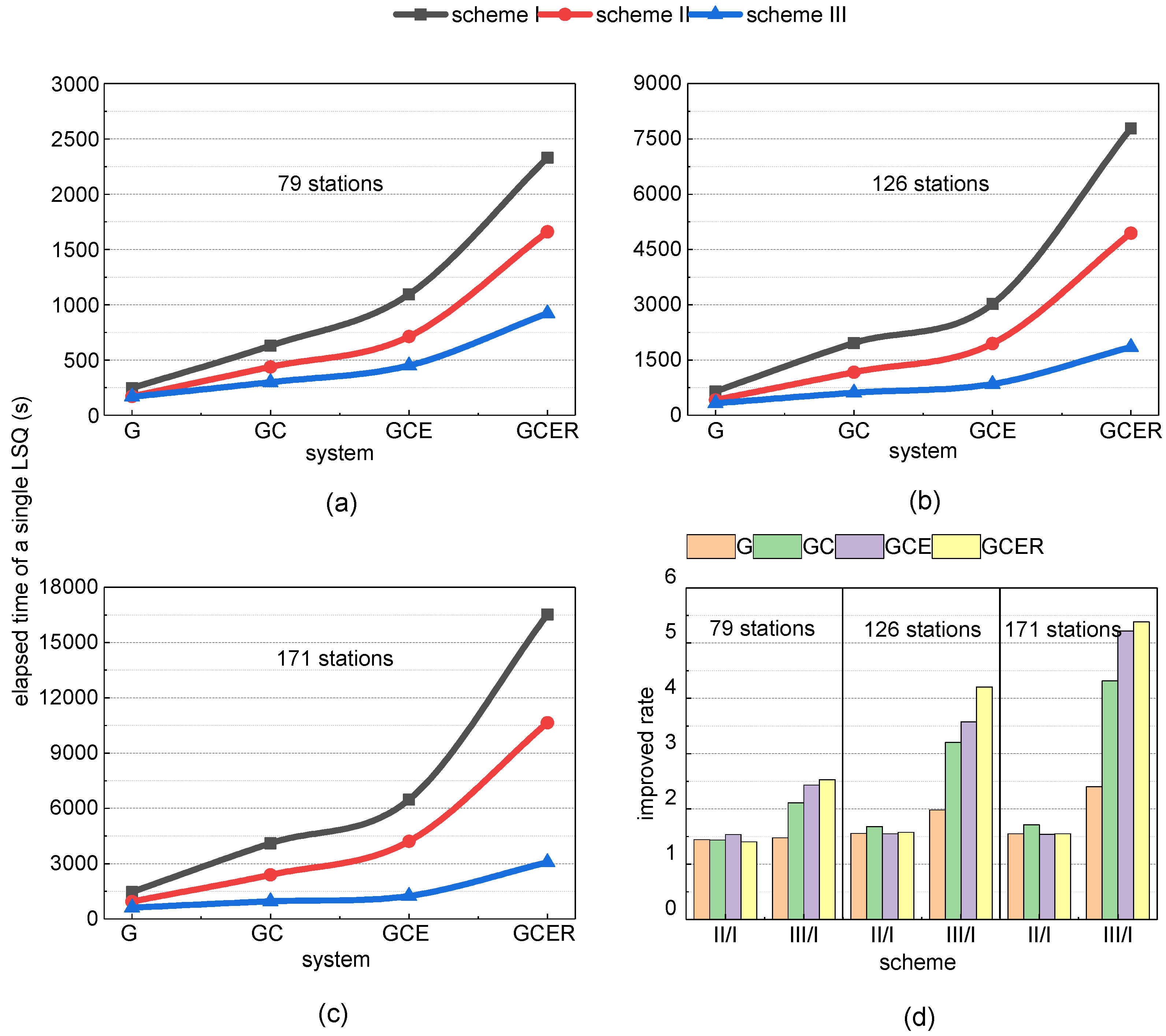
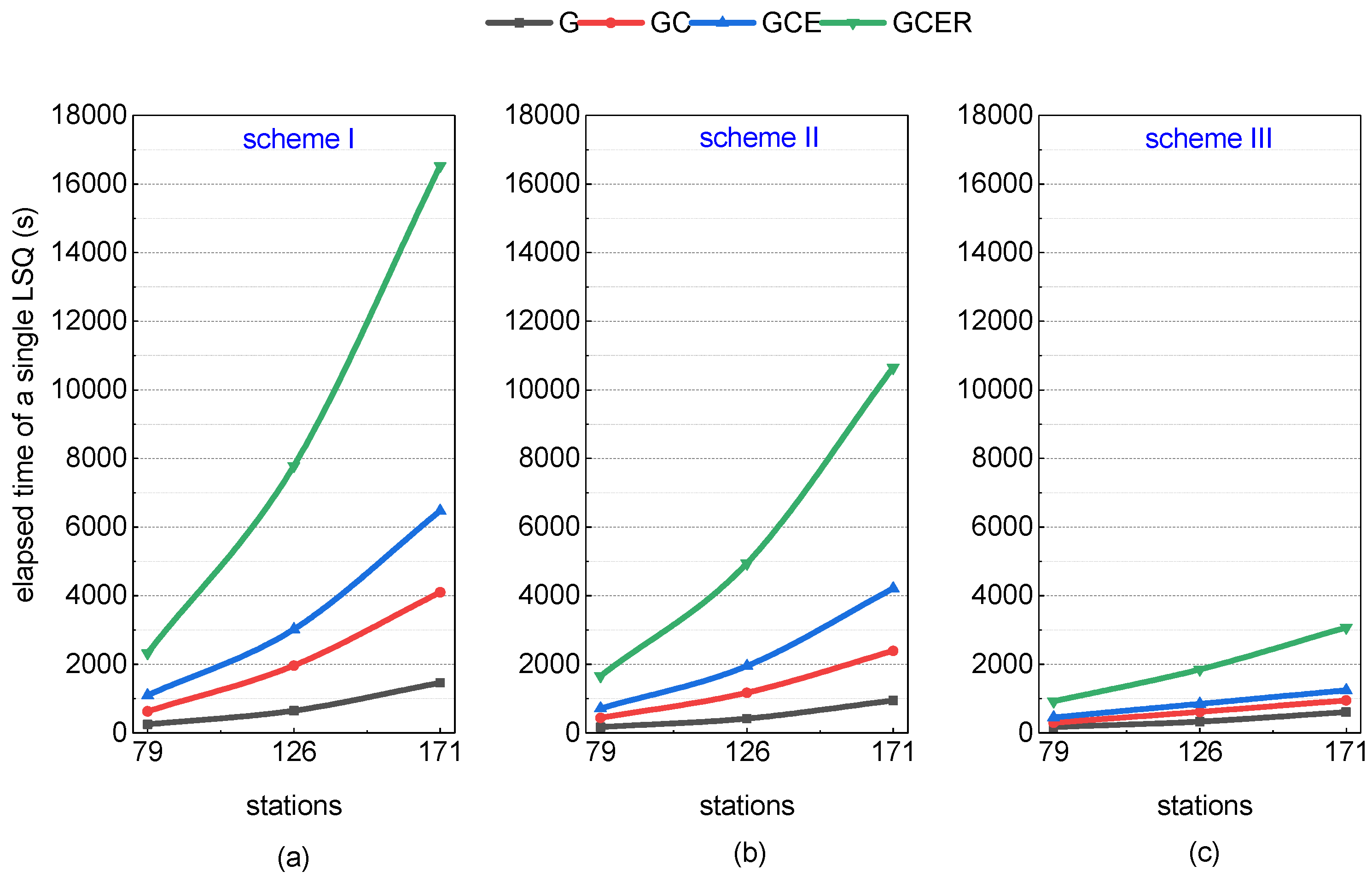
- Considering the classical estimation method based on the “one-by-one” elimination of “inactive” parameters had great success in huge GNSS networks POD, it was chosen as a reference group, named Scheme I;
- The “one-by-one” elimination method could be assisted with OpenMP to realize parallel computing, hence further improving the efficiency of multi-GNSS-integrated POD. Four threads were used to perform parameter elimination in parallel, named Scheme II;
- The improved estimation method based on the oneAPI HPC library was named Scheme III.
5. Validation of the Multi-GNSS POD
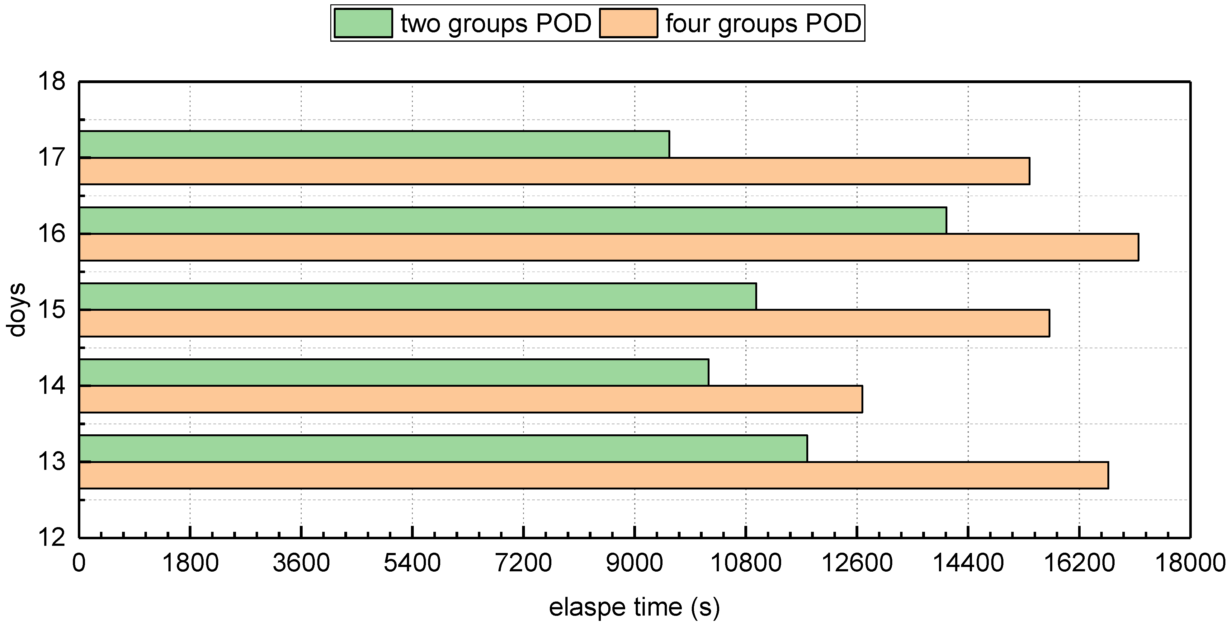
5.1. Time Consumption Analyzed for Multi-GNSS-Integrated POD
5.2. Precision for Multi-GNSS-integrated POD
6. Conclusions
Author Contributions
Funding
Data Availability Statement
Acknowledgments
Conflicts of Interest
References
- Zumberge, J.F.; Heflin, M.B.; Jefferson, D.C.; Watkins, M.M.; Webb, F.H. Precise Point Positioning for the Efficient and Robust Analysis of GPS Data from Large Networks. J. Geophys. Res. Solid Earth 1997, 102, 5005–5017. [Google Scholar] [CrossRef]
- Bahadur, B. A Study on the Real-Time Code-Based GNSS Positioning with Android Smartphones. Measurement 2022, 194, 111078. [Google Scholar] [CrossRef]
- Yan, X.; Liu, C.; Jiang, M.; Yang, M.; Feng, W.; Zhong, M.; Peng, L. Performance Analysis of Oceanographic Research Vessel Precise Point Positioning Based on BDS/GNSS RTK Receivers. Measurement 2023, 211, 112637. [Google Scholar] [CrossRef]
- Li, X.; Ge, M.; Dai, X.; Ren, X.; Fritsche, M.; Wickert, J.; Schuh, H. Accuracy and Reliability of Multi-GNSS Real-Time Precise Positioning: GPS, GLONASS, BeiDou, and Galileo. J. Geod. 2015, 89, 607–635. [Google Scholar] [CrossRef]
- Montenbruck, O.; Steigenberger, P.; Prange, L.; Deng, Z.; Zhao, Q.; Perosanz, F.; Romero, I.; Noll, C.; Stürze, A.; Weber, G.; et al. The Multi-GNSS Experiment (MGEX) of the International GNSS Service (IGS)–Achievements, Prospects and Challenges. Adv. Space Res. 2017, 59, 1671–1697. [Google Scholar] [CrossRef]
- Wu, Z.; Wang, Q.; Yu, Z.; Hu, C.; Liu, H.; Han, S. Modeling and Performance Assessment of Precise Point Positioning with Multi-Frequency GNSS Signals. Measurement 2022, 201, 111687. [Google Scholar] [CrossRef]
- Dow, J.M.; Neilan, R.E.; Rizos, C. The International GNSS Service in a Changing Landscape of Global Navigation Satellite Systems. J. Geod. 2009, 83, 191–198. [Google Scholar] [CrossRef]
- Prange, L.; Villiger, A.; Sidorov, D.; Schaer, S.; Beutler, G.; Dach, R.; Jäggi, A. Overview of CODE’s MGEX Solution with the Focus on Galileo. Adv. Space Res. 2020, 66, 2786–2798. [Google Scholar] [CrossRef]
- Steigenberger, P.; Rothacher, M.; Dietrich, R.; Fritsche, M.; Rülke, A.; Vey, S. Reprocessing of a Global GPS Network. J. Geophys. Res. Solid Earth 2006, 111, 3747. [Google Scholar] [CrossRef]
- Chen, H.; Jiang, W.; Ge, M.; Wickert, J.; Schuh, H. An Enhanced Strategy for GNSS Data Processing of Massive Networks. J. Geod. 2014, 88, 857–867. [Google Scholar] [CrossRef]
- Xie, W.; Huang, G.; Fu, W.; Shu, B.; Cui, B.; Li, M.; Yue, F. A Quality Control Method Based on Improved IQR for Estimating Multi-GNSS Real-Time Satellite Clock Offset. Measurement 2022, 201, 111695. [Google Scholar] [CrossRef]
- Steigenberger, P.; Fritsche, M.; Dach, R.; Schmid, R.; Montenbruck, O.; Uhlemann, M.; Prange, L. Estimation of Satellite Antenna Phase Center Offsets for Galileo. J. Geod. 2016, 90, 773–785. [Google Scholar] [CrossRef]
- Huang, G.; Yan, X.; Zhang, Q.; Liu, C.; Wang, L.; Qin, Z. Estimation of Antenna Phase Center Offset for BDS IGSO and MEO Satellites. GPS Solut. 2018, 22, 49. [Google Scholar] [CrossRef]
- Yan, X.; Huang, G.; Zhang, Q.; Wang, L.; Qin, Z.; Xie, S. Estimation of the Antenna Phase Center Correction Model for the BeiDou-3 MEO Satellites. Remote Sens. 2019, 11, 2850. [Google Scholar] [CrossRef]
- Rodriguez-Solano, C.J.; Hugentobler, U.; Steigenberger, P.; Bloßfeld, M.; Fritsche, M. Reducing the Draconitic Errors in GNSS Geodetic Products. J. Geod. 2014, 88, 559–574. [Google Scholar] [CrossRef]
- Montenbruck, O.; Steigenberger, P.; Hugentobler, U. Enhanced Solar Radiation Pressure Modeling for Galileo Satellites. J. Geod. 2015, 89, 283–297. [Google Scholar] [CrossRef]
- Yan, X.; Liu, C.; Huang, G.; Zhang, Q.; Wang, L.; Qin, Z.; Xie, S. A Priori Solar Radiation Pressure Model for BeiDou-3 MEO Satellites. Remote Sens. 2019, 11, 1605. [Google Scholar] [CrossRef]
- Ge, M.; Gendt, G.; Dick, G.; Zhang, F.P.; Rothacher, M. A New Data Processing Strategy for Huge GNSS Global Networks. J. Geod. 2006, 80, 199–203. [Google Scholar] [CrossRef]
- Prange, L.; Orliac, E.; Dach, R.; Arnold, D.; Beutler, G.; Schaer, S.; Jäggi, A. CODE’s Five-System Orbit and Clock Solution—The Challenges of Multi-GNSS Data Analysis. J. Geod. 2017, 91, 345–360. [Google Scholar] [CrossRef]
- Guo, J.; Xu, X.; Zhao, Q.; Liu, J. Precise Orbit Determination for Quad-Constellation Satellites at Wuhan University: Strategy, Result Validation, and Comparison. J. Geod. 2016, 90, 143–159. [Google Scholar] [CrossRef]
- Zhu, S.; Reigber, C.; König, R. Integrated Adjustment of CHAMP, GRACE, and GPS Data. J. Geod. 2004, 78, 103–108. [Google Scholar] [CrossRef]
- Li, B.; Ge, H.; Ge, M.; Nie, L.; Shen, Y.; Schuh, H. LEO Enhanced Global Navigation Satellite System (LeGNSS) for Real-Time Precise Positioning Services. Adv. Space Res. 2019, 63, 73–93. [Google Scholar] [CrossRef]
- Li, X.; Zhang, K.; Ma, F.; Zhang, W.; Zhang, Q.; Qin, Y.; Zhang, H.; Meng, Y.; Bian, L. Integrated Precise Orbit Determination of Multi- GNSS and Large LEO Constellations. Remote Sens. 2019, 11, 2514. [Google Scholar] [CrossRef]
- Serpelloni, E.; Casula, G.; Galvani, A.; Anzidei, M.; Baldi, P. Data Analysis of Permanent GPS Networks in Italy and Surrounding Region: Application of a Distributed Processing Approach. Ann. Geophys. 2006, 49, 897–928. [Google Scholar] [CrossRef]
- Boomkamp, H.; König, R. Bigger, Better, Faster POD Position Paper for Session on Precise Orbit Determination. In Proceedings of the IGS Workshop and Symposium, Berne, Switzerland, 1–5 March 2004; Volume 10. Available online: ftp://192.134.134.6/pub/igs/igscb/resource/pubs/04_rtberne/cdrom/Session9/9_0_Boomkamp.pdf (accessed on 31 February 2022).
- Li, L.; Lu, Z.; Chen, Z.; Cui, Y.; Kuang, Y.; Wang, F. Parallel Computation of Regional CORS Network Corrections Based on Ionospheric-Free PPP. GPS Solut. 2019, 23, 70. [Google Scholar] [CrossRef]
- Cui, Y.; Chen, Z.; Li, L.; Zhang, Q.; Luo, S.; Lu, Z. An Efficient Parallel Computing Strategy for the Processing of Large GNSS Network Datasets. GPS Solut. 2021, 25, 36. [Google Scholar] [CrossRef]
- Costa, J.J.; Cortes, T.; Martorell, X.; Ayguade, E.; Labarta, J. Running OpenMP Applications Efficiently on an Everything-Shared SDSM. J. Parallel Distrib. Comput. 2006, 66, 647–658. [Google Scholar] [CrossRef]
- Mironov, V.; Alexeev, Y.; Keipert, K.; D’mello, M.; Moskovsky, A.; Gordon, M.S. An Efficient MPI/OpenMP Parallelization of the Hartree-Fock Method for the Second Generation of Intel® Xeon PhiTM Processor. In Proceedings of the International Conference for High Performance Computing, Networking, Storage and Analysis, SC 2017, Denver, CO, USA, 12–17 November 2017; Association for Computing Machinery, Inc.: New York, NY, USA, 2017. [Google Scholar]
- Kuang, K.; Zhang, S.; Li, J. Real-Time GPS Satellite Orbit and Clock Estimation Based on OpenMP. Adv. Space Res. 2019, 63, 2378–2386. [Google Scholar] [CrossRef]
- Chen, X.; Ge, M.; Hugentobler, U.; Schuh, H. A New Parallel Algorithm for Improving the Computational Efficiency of Multi-GNSS Precise Orbit Determination. GPS Solut. 2022, 26, 83. [Google Scholar] [CrossRef]
- Yang, Y.; Mao, Y.; Sun, B. Basic Performance and Future Developments of BeiDou Global Navigation Satellite System. Satell. Navig. 2020, 1, 1. [Google Scholar] [CrossRef]
- Intel oneAPI Intel®-Optimized Math Library for Numerical Computing. Available online: https://www.intel.com/content/www/us/en/developer/articles.html (accessed on 31 February 2022).
- Leick, A.; Rapoport, L.; Tatarnikov, D. GPS Satellite Surveying; Wiley: Hoboken, NJ, USA, 2015. [Google Scholar]
- Li, X.; Ge, M.; Lu, C.; Zhang, Y.; Wang, R.; Wickert, J.; Schuh, H. High-Rate GPS Seismology Using Real-Time Precise Point Positioning with Ambiguity Resolution. IEEE Trans. Geosci. Remote Sens. 2014, 52, 6165–6180. [Google Scholar] [CrossRef]
- Ren, X.; Chen, J.; Li, X.; Zhang, X. Ionospheric Total Electron Content Estimation Using GNSS Carrier Phase Observations Based on Zero-Difference Integer Ambiguity: Methodology and Assessment. IEEE Trans. Geosci. Remote Sens. 2021, 59, 817–830. [Google Scholar] [CrossRef]
- Beutler, G.; Brockmann, E.; Gurtner, W.; Hugentobler, U.; Mervart, L.; Rothacher, M.; Verdun, A. Extended Orbit Modeling Techniques at the CODE Processing Center of the International GPS Service for Geodynamics (IGS): Theory and Initial Results. Manuscr. Geod. 1994, 19, 367–386. [Google Scholar]
- Arnold, D.; Meindl, M.; Beutler, G.; Dach, R.; Schaer, S.; Lutz, S.; Prange, L.; Sośnica, K.; Mervart, L.; Jäggi, A. CODE’s New Solar Radiation Pressure Model for GNSS Orbit Determination. J. Geod. 2015, 89, 775–791. [Google Scholar] [CrossRef]
- Blewitt, G. An Automatic Editing Algorithm for GPS Data. Geophys. Res. Lett. 1990, 17, 199–202. [Google Scholar] [CrossRef]
- Ge, M.; Gendt, G.; Rothacher, M.; Shi, C.; Liu, J. Resolution of GPS Carrier-Phase Ambiguities in Precise Point Positioning (PPP) with Daily Observations. J. Geod. 2008, 82, 389–399. [Google Scholar] [CrossRef]
- Schaer, S.; Villiger, A.; Arnold, D.; Dach, R.; Prange, L.; Jäggi, A. The CODE Ambiguity-Fixed Clock and Phase Bias Analysis Products: Generation, Properties, and Performance. J. Geod. 2021, 95, 81. [Google Scholar] [CrossRef]
- Liu, X.; Jiang, W.; Li, P.; Deng, Z.; Ge, M.; Schuh, H. An Extended Inter-System Biases Model for Multi-GNSS Precise Point Positioning. Measurement 2023, 206, 112306. [Google Scholar] [CrossRef]
- IGS MGEX International GNSS Service, GNSS Constellations. Available online: http://mgex.igs.org/index.php#Constellations (accessed on 31 October 2019).
- Saastamoinen, J. Atmospheric correction for the troposphere and stratosphere in radio ranging satellites. Use Artifical Satell. Geod. 1972, 15, 247–251. [Google Scholar]
- Boehm, J.; Niell, A.; Tregoning, P.; Schuh, H. Global Mapping Function (GMF): A New Empirical Mapping Function Based on Numerical Weather Model Data. Geophys. Res. Lett. 2006, 33, L07304. [Google Scholar] [CrossRef]
- Altamimi, Z.; Rebischung, P.; Métivier, L.; Collilieux, X. ITRF2014: A New Release of the International Terrestrial Reference Frame Modeling Nonlinear Station Motions. J. Geophys. Res. Solid Earth 2016, 121, 6109–6131. [Google Scholar] [CrossRef]
- Villiger, A.; Dach, R.; Schaer, S.; Prange, L.; Zimmermann, F.; Kuhlmann, H.; Wübbena, G.; Schmitz, M.; Beutler, G.; Jäggi, A. GNSS Scale Determination Using Calibrated Receiver and Galileo Satellite Antenna Patterns. J. Geod. 2020, 94, 93. [Google Scholar] [CrossRef]


| Type | Descriptions |
|---|---|
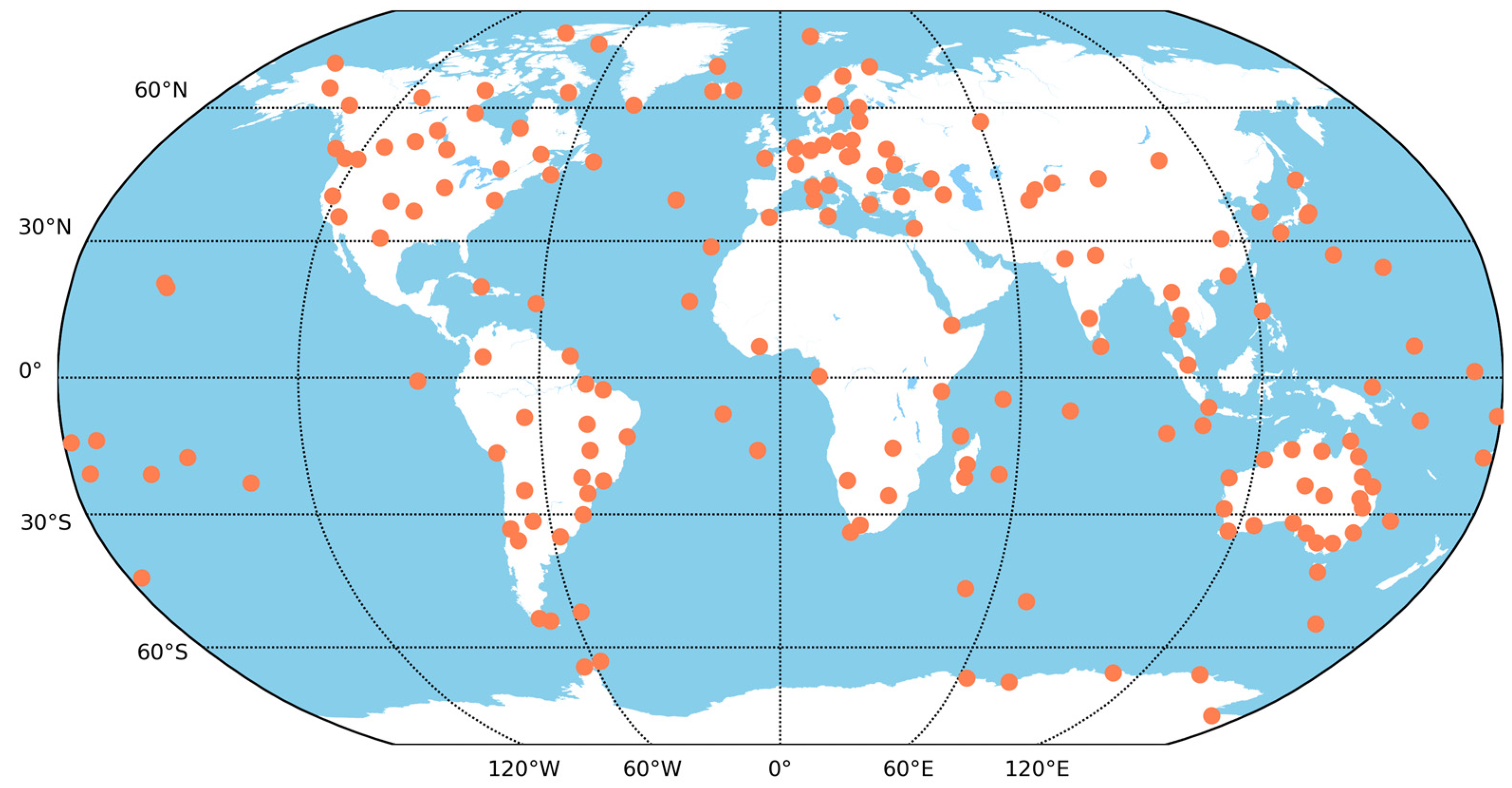
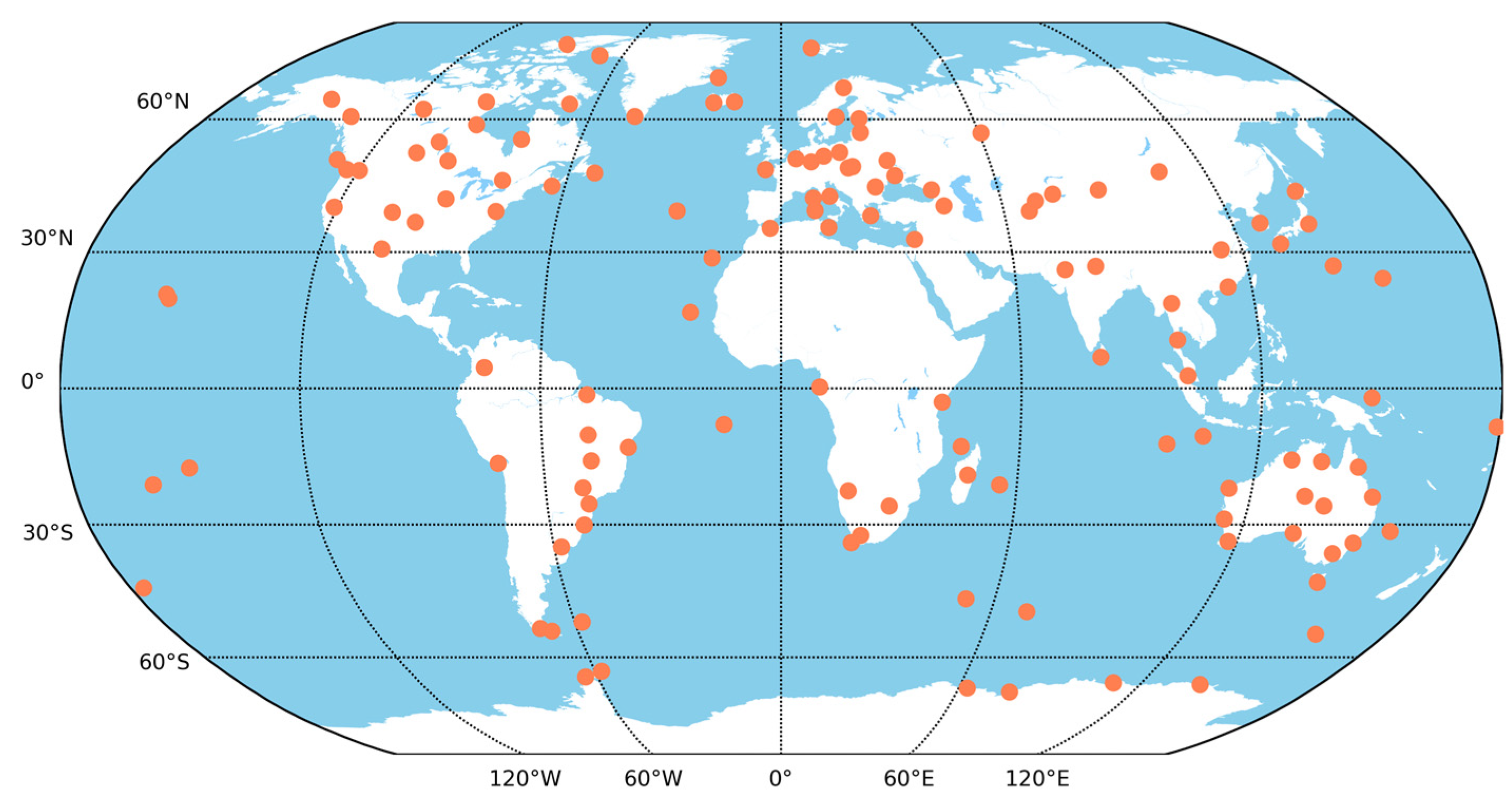
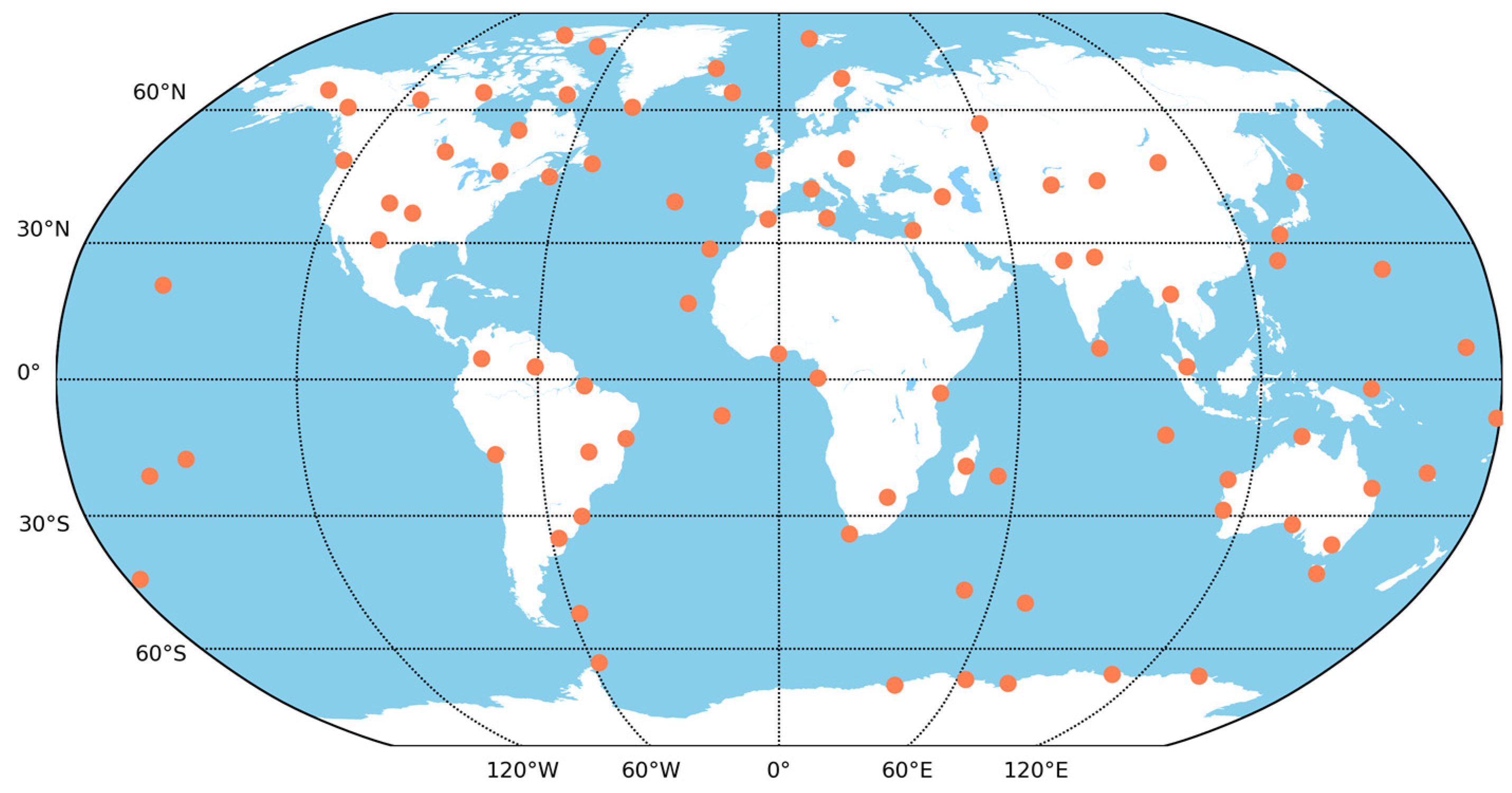
| stations | IGS/MGEX station network [43]; |
| Period | Days of year (DOYs) from 013 to 019, 2022; |
| Observations | zero-difference carrier phase and pseudo-range elevation weight; cut-off is 7°; |
| orbital arc | 24 h; |
| Solar radiation pressure model | GPS/GLONASS: ECOM2 [38]; Galileo: ECOM1+a priori model [16,37]; BDS2: ECOM1; BDS3: ECOM1 + a priori model [17]; |
| Inter-system biases (ISB) and Inter-frequency biases (IFB) | ISB between BDS2/3 and GPS, Galileo, and GPS; constant parameter per station; IFB per satellite and station pair between GLONASS and GPS; Constraint that sum of all ISBs and IFBs are zero was added; |
| Ionospheric delay | Ionosphere-free (IF) combination; GPS: L1/L2; BDS: B1I/B3I; Galileo: E1/E5a; GLONASS: R01/R02; |
| Tropospheric delay | Zenith total delay (ZTD): 2-h interval; Saastamoinen [44] + Global Map Function (GMF) [45]; Horizontal gradient: 24-h interval; |
| Antenna phase center correction (PCC) | For both satellites and receivers, phase center correction model is from igs14_2196.atx [46,47]; BDS and Galileo receivers PCC was using GPS L1 and L2 instead. |
| Systems | PRN List |
|---|---|
| GPS (G) | G01, G02, G03, G04, G05, G06, G07, G08, G09, G10, G11, G12, G13, G14, G15, G16, G17, G18, G19, G20, G21, G22, G24, G25, G26, G27, G28, G29, G30, G31, G32 |
| GLONASS (R) | R01, R02, R03, R04, R05, R06, R07, R08, R09, R10, R11, R12, R13, R14, R15, R17, R18, R19, R20, R21, R22, R23, R24 |
| BDS (C) | C01, C02, C03, C04, C05, C06, C07, C08, C09, C10, C11, C12, C13, C14, C16, C19, C20, C21, C22, C23, C24, C25, C26, C27, C28, C29, C30, C32, C33, C34, C35, C36, C37, C38, C39, C40, C41, C42, C43, C44, C45, C46 |
| Galileo (E) | E01, E02, E03, E04, E05, E07, E08, E09, E11, E12, E13, E15, E18, E19, E21, E24, E25, E26, E27, E30, E31, E33, E36 |
| Systems | 79 Stations | 126 Stations | 171 Stations | ||||||
|---|---|---|---|---|---|---|---|---|---|
| I | II | III | I | II | III | I | II | III | |
| G | 0:04:06 | 0:02:50 | 0:02:47 | 0:10:46 | 0:06:55 | 0:05:26 | 0:24:22 | 0:15:43 | 0:10:08 |
| GC | 0:10:29 | 0:07:18 | 0:04:58 | 0:32:42 | 0:19:30 | 0:10:13 | 1:08:19 | 0:39:53 | 0:15:50 |
| GCE | 0:18:14 | 0:11:52 | 0:07:30 | 0:50:21 | 0:32:27 | 0:14:05 | 1:47:55 | 1:10:10 | 0:20:41 |
| GCER | 0:38:51 | 0:27:40 | 0:15:22 | 2:09:45 | 1:22:23 | 0:30:50 | 4:35:25 | 2:57:30 | 0:51:11 |
| Systems | 79 Stations | 126 Stations | 171 Stations | |||
|---|---|---|---|---|---|---|
| II/I | III/I | II/I | III/I | II/I | III/I | |
| G | 1.45 | 1.48 | 1.56 | 1.98 | 1.55 | 2.40 |
| GC | 1.44 | 2.11 | 1.68 | 3.20 | 1.71 | 4.32 |
| GCE | 1.54 | 2.43 | 1.55 | 3.58 | 1.54 | 5.22 |
| GCER | 1.40 | 2.53 | 1.57 | 4.21 | 1.55 | 5.38 |
| Systems | 79 Stations | 126 Stations | 171 Stations | ||||||
|---|---|---|---|---|---|---|---|---|---|
| I | II | III | I | II | III | I | II | III | |
| G | 0:37:14 | 0:32:10 | 0:31:58 | 1:08:54 | 0:53:30 | 0:47:34 | 2:07:50 | 1:33:14 | 1:10:54 |
| GC | 1:07:14 | 0:54:30 | 0:45:10 | 2:42:09 | 1:49:21 | 1:12:13 | 5:09:54 | 3:16:09 | 1:39:57 |
| GCE | 1:43:15 | 1:17:47 | 1:00:19 | 3:58:16 | 2:46:40 | 1:33:12 | 7:54:11 | 5:23:11 | 2:05:15 |
| GCER | 3:08:22 | 2:23:38 | 1:34:26 | 9:18:58 | 6:09:30 | 2:43:18 | 19:09:28 | 12:37:48 | 4:12:32 |
| Satellites | 79 Stations | 126 Stations | 171 Stations |
|---|---|---|---|
| GPS | 1.4 | 1.3 | 1.3 |
| BDS GEO | 315.0 | 280.7 | 234.4 |
| BDS IGSO | 10.5 | 8.6 | 7.9 |
| BDS MEO | 5.3 | 4.9 | 4.9 |
| Galileo | 1.5 | 1.3 | 1.3 |
| GLONASS | 3.1 | 2.7 | 2.7 |
Disclaimer/Publisher’s Note: The statements, opinions and data contained in all publications are solely those of the individual author(s) and contributor(s) and not of MDPI and/or the editor(s). MDPI and/or the editor(s) disclaim responsibility for any injury to people or property resulting from any ideas, methods, instructions or products referred to in the content. |
© 2023 by the authors. Licensee MDPI, Basel, Switzerland. This article is an open access article distributed under the terms and conditions of the Creative Commons Attribution (CC BY) license (https://creativecommons.org/licenses/by/4.0/).
Share and Cite
Yan, X.; Liu, C.; Yang, M.; Feng, W.; Zhong, M. An Improved Parameter Estimation Method for High-Efficiency Multi-GNSS-Integrated Orbit Determination. Remote Sens. 2023, 15, 2635. https://doi.org/10.3390/rs15102635
Yan X, Liu C, Yang M, Feng W, Zhong M. An Improved Parameter Estimation Method for High-Efficiency Multi-GNSS-Integrated Orbit Determination. Remote Sensing. 2023; 15(10):2635. https://doi.org/10.3390/rs15102635
Chicago/Turabian StyleYan, Xingyuan, Chenchen Liu, Meng Yang, Wei Feng, and Min Zhong. 2023. "An Improved Parameter Estimation Method for High-Efficiency Multi-GNSS-Integrated Orbit Determination" Remote Sensing 15, no. 10: 2635. https://doi.org/10.3390/rs15102635