Article

Impact of Horizontal Resolution on the Robustness of Radiation Emulators in a Numerical Weather Prediction Model

1
National Institute of Meteorological Sciences, Korea Meteorological Administration, Seogwipo-si 63568, Republic of Korea
2
Department of Atmospheric Sciences, Center for Atmospheric Remote Sensing (CARE), Kyungpook National University, Daegu 41566, Republic of Korea
*
Author to whom correspondence should be addressed.
Remote Sens. 2023, 15(10), 2637; https://doi.org/10.3390/rs15102637
Submission received: 4 April 2023 / Revised: 3 May 2023 / Accepted: 15 May 2023 / Published: 18 May 2023

Abstract

:
Developing a machine-learning-based radiative transfer emulator in a weather forecasting model is valuable because it can significantly improve the computational speed of forecasting severe weather events. To replace the radiative transfer parameterization in the weather forecasting model, the universal applicability of the radiation emulator is essential, indicating a transition from the research to the operational level. This study investigates the degradation of the forecast accuracy of the radiation emulator for the Korea peninsula when it is tested at different horizontal resolutions (100–0.25 km) concerning the accuracy attained at the training resolution (5 km) for universal applications. In real-case simulations (100–5 km), the forecast errors of radiative fluxes and precipitation were reduced at coarse resolutions. Ideal-case simulations (5–0.25 km) showed larger errors in heating rates and fluxes at fine resolutions, implying the difficulty in predicting heating rates and fluxes at cloud-resolving scales. However, all simulations maintained an appropriate accuracy range compared with observations in real-case simulations or the infrequent use of radiative transfer parameterization in ideal-case simulations. These findings demonstrate the feasibility of a universal radiation emulator associated with different resolutions/models and emphasize the importance of emulating high-resolution modeling in the future.

1. Introduction

Because the parameterization of the radiative transfer process accounts for the largest computation burden in atmospheric prediction models (over 80% [1,2]), machine-learning emulators imitating radiative transfer processes with a faster computational speed have been actively developed. Initial studies were confined to imitating the radiative transfer model (RTM) under clear sky simulation or ideal conditions that can be difficult to apply universally [3,4,5,6,7,8,9]. For RTM emulation studies, advanced machine-learning techniques, in addition to the common neural network (NN) based on the feed-forward multi-layer perceptron (such as the random forest ([10]), convolutional neural network (CNN [4]), recurrent neural network (RNN [9]), and U-net++ model [6]), have been actively used. Emulation studies have attempted to replace radiative transfer parameterizations in atmospheric weather/climate forecasting models [1,2,10,11,12,13,14,15,16,17,18,19,20,21]. These emulator studies have reported sufficient speed improvements of 10 to 100 times compared with theoretical radiation schemes based on discrete bands [22,23,24,25,26].
Although the speed improvement by the RTM emulator was confined to the radiation process only, the radiation emulator in the numerical weather prediction (NWP) model can further speed up the entire numerical prediction system, benefiting many applications in which urgent weather forecasting (e.g., typhoon, flood, and heavy snowfall forecasting) is essential. In addition, because the radiation emulator is linked to many dynamic and physical variables in the NWP model or general circulation model (GCM), the emulator can produce tremendous outputs (e.g., weather charts at various levels) indirectly linked with radiative transfer processes at a faster speed. Therefore, the radiation emulator in numerical prediction models (online test) is incomparably valuable for broad applications compared to the RTM emulator (offline test) not linked to numerical models. Ref. [11] first developed a NN emulator functioning 50–80 times faster than longwave (LW) parameterization in the Community Atmospheric Model (CAM) with T42 resolution (~300 km). The emulation for shortwave (SW) parameterization, which was 20-fold faster, was further included under the same CAM [12]. Ref. [10] for different machine-learning methods and [13] for compound parameterization were conducted under the same CAM framework. NN emulators for both LW and SW can improve the computational speed of radiative transfer calculations by approximately 30 times and the total computation time by a maximum of 25% under the Climate Forecast System (CFS) model with T126 resolution (~100 km) [14]. Ref. [16] developed an NN emulator with multiple hidden layers that can accelerate the computational speed of the radiation process by a maximum of 10 times under a super-parameterized energy exascale earth system model (SP-E3SM) with a 1° horizontal resolution (~100 km). Ref. [15] further reported a speedup of approximately 40 times for the radiation process and a total reduction in computation time by a maximum of 18% under the Global Forecast System (GFS) model with T574 resolution (~25 km). Recently, Ref. [17] demonstrated the universal performance of a radiation emulator developed for the CFS model at the global scale [14] by applying it to the GFS model. Although the current GFS model has a 13 km resolution compared to the 100 km resolution of CFS, they kept the resolution at 100 km as in the GFS experiment. In contrast to global models, radiation emulators for the Korean local model with a 5 km resolution, called the Korea Local Analysis and Prediction System (KLAPS [27]), were developed, showing a significant speedup in the radiation process by 60-fold and 87% reduction in total computation time [2,18,19,20]. Ref. [1] developed a unique radiation emulator with speed improvements for the radiation process by 20–100 times and 82–86% reduction in total model time for a cloud-resolving model (CRM) with a 0.25 km resolution. However, their result was limited to an ideal case of a 6 h forecast in the daytime. Because previous studies on radiation emulators were conducted in different modeling frameworks based on different horizontal resolutions (from GCM to CRM), the absolute errors found in the literature are difficult to compare. Because atmospheric profiles at a coarse horizontal resolution are less extreme, they can be trained over a smaller range than cloud-resolving, thereby facilitating the development of a radiation simulation. The same effects diminish the detail through the smoothing effect of fine resolution. However, the as-developed model might not ensure better performance in terms of universal applicability. Therefore, the impact of horizontal resolutions on the forecast accuracy of radiation emulators needs to be comprehensively investigated. To evaluate the accuracy of an emulator, various aspects need to be validated, such as comparison with a control simulation that uses the original radiative transfer parameterization [10,11,12,13,14,15,16,17] and evaluations with the infrequent use of radiative transfer parameterization and observations [1,2,18,19,20]. Because observations for an ideal-case simulation are absent, the infrequent use of radiative transfer parameterization can be a benchmark for evaluating the forecast accuracy of a radiation emulator at the same computational speed.
The horizontal resolution effect in the NWP model is a topic that many atmospheric scientists are interested in. For example, precipitation in the NWP model is implicitly determined by cumulus parameterization at coarse horizontal resolutions (e.g., above 100 km), whereas it is explicitly calculated using cloud microphysics parameterization at convection-permitting scales, typically at resolutions of several kilometers. Owing to the spatial smoothing effect, precipitation forecasting at coarse resolution appears to be more accurate compared with that at fine resolution [28,29]; however, precipitation forecasting at fine resolution is still important. In contrast, the forecast accuracy at coarse resolution for surface temperature is lower than that at fine resolution [30,31] because the smoothing effect at coarse resolution hinders the realistic prediction of temperature variability. The contrast associated with horizontal resolutions can lead to a conjecture that the climate models with 100–300 km resolutions [10,11,12,13,14,15,16,17] will exhibit a different behavior compared with those of the convection-permitting NWP model with a 5 km resolution [2,18,19,20] or CRM with a 0.25 km resolution [1]. This may eventually affect the performance of the radiative transfer emulator. Although they are not linked with numerical forecasting models, emulation studies for RTM have used datasets based on horizontal resolutions of 80 km [4,9], 30 km [8], 13 km [6], and various data sources [5,7]. However, these studies used different numerical models and machine-learning methods, and it is difficult to conclude which studies showed improved results. Furthermore, all previous radiation emulators were evaluated at the same resolution as the trained horizontal resolution. Because the horizontal resolution of datasets and targeting models can be changed according to institutional policy or user interest in the trained version, the universal robustness of the developed radiation emulators at different horizontal scales should be satisfied for applying them to modeling systems with various horizontal resolutions.
The universal applicability of radiation emulators, partially demonstrated by [17,20], is associated with the changes in numerical models (CFS to GFS) and microphysics parameterizations along with different models (real-case to ideal-case simulations). However, the effect of horizontal resolution on the robustness of the radiation emulators remains unknown. Therefore, this study aims to investigate the universal performance of a radiation emulator with a 5 km resolution developed by [19] when applied to different horizontal resolutions for climate and cloud-resolving simulations (100 km to 0.25 km). As in [20], the trained results from three-dimensional real-case simulations were applied to two-dimensional idealized squall line simulation. This ideal-case simulation is particularly important in predicting the evolution of clouds and precipitation because many cloud microphysics schemes are developed in the ideal framework [32,33,34,35]. It is a good testbed for evaluating the radiative transfer emulator because radiative transfer processes are closely related to cloud processes. These quantitative analyses can provide insights into the extent to which the emulator can be used across horizontal resolutions for a potential use in the operational NWP model, along with suggesting a future development direction for radiation emulators capable of operating at fine resolutions.

2. Data and Methods

2.1. NN Emulator

This study used the NN radiation scheme developed by [19] for the KLAPS model over the Korean peninsula. For a detailed flowchart of NN development, see Figure S1 of the supporting information in [1]. The emulator imitated the RRTMG-K radiative transfer parameterization [24], which is an updated version of the rapid RTM for GCMs (RRTMG [23]) with LW of 14 bands and 256 g-points and SW of 16 bands and 224 g-points. In [19], 288 million input-output pairs were used as training sets based on random sampling for 2009–2019 with 1 h intervals. Training sets comprised 96 categories for 12 months, land/ocean, clear/cloud, and LW/SW. The input variables used were vertical profiles of pressure, temperature, water vapor, ozone, and cloud fraction, in addition to skin temperature and surface emissivity (LW), as well as insolation and surface albedo (SW). The output variables used were all-sky heating rate profiles, upward fluxes at the top and bottom of the atmosphere, and downward flux at the bottom. Hereafter, the LW/SW fluxes in this study refer to the average of the three fluxes at the top and bottom. The individual fluxes as output variables at the top or bottom were also considered for statistical analyses.
The NN approximated the nonlinear relationship between input and output based on 90 neurons and a single hidden layer. This neuron network size was also previously used in the literature for developing an efficient radiation emulator with appropriate accuracy [2,18,19,20]. The use of more neurons and hidden layers can increase the computational speed of the radiative transfer calculation by the emulator, although it can further improve the accuracy of the emulator. Ref. [19] noted that single and two hidden layers were the most appropriate at the 60-fold speedup condition for the ideal-case and real-case simulations, respectively, in reducing the forecast accuracy of LW/SW fluxes by 19.1% (ideal-case) and 4.8% (real case). This study selected the single hidden layer. Appropriate batch size and learning rate can optimize NN training based on parallel learning. This study used a batch size of 500 and a learning rate of 0.05 from [19]. Ref. [19] showed that the forecast errors of LW/SW fluxes were reduced by 8.2–11.6% through offline sensitivity experiments on batch sizes and learning rates. Although the learning rate at a given batch size can be further optimized by more expensive experiments (such as those performed by [21]), such an approach was not followed in our present study because the forecast accuracy of LW/SW fluxes in online testing appeared to be saturated regardless of the learning rates. Furthermore, although the use of batch size smaller than 500 (i.e., mini-batch size) may improve the NN training, its practicality is limited because training time is increased while less parallel learning is achieved. This study also used the tangent hyperbolic (Tanh) activation function. Because the activation function is applied between input variables and the hidden layer in the emulator code, it is more important than the batch size and the learning rate that only affect the training process. Sensitivity experiments on 15 activation functions by [19] showed that the forecast errors of LW/SW fluxes improved by 12.2–13.4% using the Tanh.
For better generation, NN training was further optimized using stochastic weight averaging (SWA [36]). Because the SWA mimics an ensemble approach by using a stochastic averaging for weight coefficients while keeping the same dimension for final weight coefficients (i.e., same numerical complexity), it effectively reduces the generalization error while maintaining the computational speed of the emulator. As a result of the NN training, weight and bias coefficients (input to the hidden layer and hidden layer to output) were obtained; these were then linked to the KLAPS model. Note that the weight/bias coefficients were somewhat smoothed by applying the SWA. The radiation emulator showed an approximately 60-fold speedup compared to RRTMG-K and an 84–87% reduction in total computation time [2,19].

2.2. Numerical Experiments

The KLAPS model used in this study was based primarily on the Advanced Research of the Weather Research and Forecasting (WRF-ARW) model [37]. The physics suites other than radiative transfer parameterization were the WRF double moment 7-Class (WDM7) microphysics [35], unified Noah land surface model [37], Simplified Arakawa–Schubert cumulus modified by the Korea Institute of Atmospheric Prediction Systems [38], Shin and Hong boundary layer [39], and revised MM5 Monin–Obukhov surface layer [40]. In coarse resolutions, the effect of the cumulus scheme is dominant in determining cloud and precipitation, whereas the microphysics scheme is important in the convection-permitting simulation (e.g., 5 km). The cumulus scheme is not directly connected with the radiative transfer parameterization, whereas the microphysics scheme explicitly interacts with radiative transfer processes. The European Center for Medium-Range Weather Forecasts Reanalysis v5 (ERA5 [41]) data with 0.25° horizontal and 37 pressure-level resolutions were used for initial profiles and boundary conditions in the real-case simulation. The real-case simulation was integrated for 7 days with a 20 s time step over 5 km horizontal grids (234 × 282) based on the Lambert conformal conic projection and 40 vertical levels. The real-case simulations were initialized from the 1st, 8th, 15th, and 22nd days of each month in 2020, comprising 48 weekly cases. For these cases, the LW and SW fluxes at 3 h intervals were used to evaluate the forecast accuracy of the radiation emulator by comparing it with the control simulation (3 h intervals) based on radiative transfer parameterization (i.e., RRTMG-K). The forecast accuracy of the emulator and control results was also evaluated by comparing them with surface observations in South Korea. The 2 m air temperature (T2m) data from 713 stations were measured. Additionally, precipitation data with a 5 km resolution were derived by merging rain gauges and ground-based radar measurements (Figure 1). The precipitation data were generated by further considering radar estimations for areas where rain gauge observation was unavailable at a certain 5 km grid. The datasets were obtained from the Numerical Modeling Center at the Korea Meteorological Administration. Because the uncertainty of precipitation from radar measurements is large for regions without rain gauge observations (e.g., the ocean and North Korea), this study only considered the land region of South Korea. The observed and model precipitation values were spatially interpolated onto a regular 0.05° × 0.05° grid. Furthermore, this study considered a two-dimensional squall line experiment using the WRF model for an extreme weather event simulation [37]. However, this case study corresponds to a highly unstable situation compared to the one-year average of the real-case simulations. For example, the forecast errors of the LW/SW fluxes were 121% and 185% larger in the ideal-case simulation than in the real case [20]. This ideal simulation was forced by the default initial sounding in the WRF model and was based on 201 horizontal grids and 40 vertical levels. Furthermore, it was integrated for 24 h with a 3 s time step. The radiation emulator developed in the real-case training was applied to the ideal-case simulation to test the robustness associated with the representation error, similar to that in [20], for microphysics parameterizations. Here, the radiation emulator developed for July and land was selected among 12 months and land-ocean categories in [19], considering the maximum solar zenith angle and predefined surface condition for the ideal simulation. The radiation emulator system comprised four components for LW (day and night) and SW (day only), as well as clear and cloud areas.
To analyze the effects of resolution on universal performance of the radiation emulator, simulations were performed considering different spatial grids of 234 × 282 (5 km), 118 × 142 (10 km), 48 × 57 (25 km), 25 × 29 (50 km), 16 × 20 (75 km), and 13 × 15 (100 km), while maintaining similar spatial coverage on the Korean peninsula. The trained results with 5 km resolution were applied to 10–100 km resolutions as an independent validation. The 5 km simulation was also evaluated for the independent period (2020) and the training period (2009–2019) used in the previous study [19]. Note that the prognostic uncertainty in the NWP model can be significantly accumulated in the long-term integration. In previous studies [2,18,19,20,21], the surrounding four points around the lateral boundary were excluded from both training and testing because physically unrealistic data can appear around the lateral boundary. However, because the 100 km simulation was performed in a small domain, excluding the data around the lateral boundary between 5 km and 100 km was unfair regarding spatial coverage. This study modified the width of the relaxation zone from four grid points to one grid point, and thus, the data around the lateral boundary were also included in this study. For ideal-case simulation, 5, 3, 2, 1, 0.5, and 0.25 km resolutions were used while maintaining 201 horizontal grids.

2.3. Previous Studies on Different Resolutions

There is a trade-off between accuracy and speedup in the emulator study; thus, the accuracy of the emulator should be compared under the same (or similar) computational speed conditions. Because of this, using many neurons and hidden layers in the NN is a constraint, leading to a slowdown that is against the ultimate goal of the radiation emulator in GCMs and NWPs. Even if a study shows better accuracy using an advanced machine-learning method, an additional slowdown from the method should be contemplated. Differences in horizontal resolution further complicate the problem. Table 1 compares the offline evaluations (i.e., for independent validation sets) for all-sky LW/SW heating rates found in the literature and this study. The offline evaluates a radiative transfer error induced by the NN approximation. Although the radiative transfer process is not affected by the horizontal resolution, the spatial smoothing effect of input/output variables (i.e., infrequent extreme events at coarse resolutions) can affect the accuracy of the radiation emulator.
As shown in Table 1, Ref. [1] showed that a radiation emulator with approximately 60-fold speedup exhibited root mean square errors (RMSEs) of 1.54 K day−1 for LW heating rate and 1.13 K day−1 for LW and SW heating rates under the 0.25 km resolution; however, these errors strongly depend on the NN structure [1]. For 288 million data in real-case simulations (independent of training sets), the NN radiation scheme developed under 5 km resolution with a 60-fold speedup [2] showed the RMSEs of 0.59 K day−1 for LW heating rate, 0.22 K day−1 for SW heating rate, 4.41 W m−2 for LW flux, and 20.72 W m−2 for SW flux. These RMSEs were further reduced to 0.46 K day−1, 0.18 K day−1, 3.59 W m−2, and 19.13 W m−2, respectively, using SWA during NN training ([19]). The error for the SW heating rate in [19] was comparable to that using the RNN (0.16 K day−1) in [9], despite the huge difference in speedups for the radiative transfer process (111-fold vs. 4-fold). Note that the 60-fold speedup for both LW and SW processes can be divided into approximately 30 and 111 times for LW and SW, respectively [2]. Recently, Ref. [42] showed 15.71-fold and 2.16-fold speedups using FC (Fully connected) that is the same model used in this study and Bi-LSTM, with RMSEs of SW heating rates of 1.172 K day−1 and 0.277 K day−1, RMSEs of LW heating rates of 2.035 K day−1 and 0.337 K day−1, respectively. Despite implementation with more complex NN structures such as Bi-LSTM, which is used as the bridge between WRF and ML model for inference, it represented that it needed more optimization for speedup and accuracy. In a similar study, Ref. [4] built the instance model that implements CNN by wrapping the radiation model with python. However, even though the technologies used were outstanding, the primary goal (speedup) of emulator development was lost. That is why many works of literature tried a simple NN model for emulator development. In GCM studies, the RMSEs for the LW and SW heating rates in the offline tests were 0.34 K day−1 and 0.19 K day−1 in 300 km resolution (CAM), 0.49 K day−1 and 0.20 K day−1 in 100 km resolution (CFS), and 0.52 K day−1 and 0.26 K day−1 in 25 km resolution (GFS), respectively [14]. The radiation emulators for CFS and GFS were 30–40 times faster than RRTMG, similar to RRTMG-K targeted in [1,2,18,19,20,21]. Because the GCM studies were performed in the same group using the same NN technique and input–output structure, we suspect that the heating rate errors by the emulator reduced when the horizontal resolution became coarse, even considering the difference in simulation cases. The results obtained by Krasnopolsky and coworkers using 0.4 million data points (both LW and SW) were based on individual NN training for each GCM model. However, Refs. [2,19] used numerous training sets (288 million data) for a small area (i.e., Korea). Because the representation error can be reduced by using more datasets covering natural variability, despite the 5 km resolution, the RMSEs of the LW and SW heating rates in [19] were smaller than those in [14,15].
Numerical errors caused by a radiation emulator can be rapidly amplified during long-term integration into GCMs or NWPs (called online prognostic testing). For an ideal-case simulation under 0.25 km resolution, the RMSEs of LW/SW fluxes were amplified by 135% and 72%, respectively, during 6 h forecasts (7200-time steps) compared with the offline testing results [1]. For a real-case simulation with 5 km resolution, the RMSEs for LW/SW fluxes during 1-day forecasts (4320-time steps) increased by 84% and 136%, respectively [2]. For 7-day forecasts (30,240-time steps), the RMSEs for LW/SW fluxes increased further by 148% and 215%, respectively [19]. From these results, the numerical errors of the radiation emulator can be amplified more in the case of seasonal or inter-annual predictions based on the GCM. However, because the GCM forecasts are evaluated at monthly or yearly scales in contrast to the hourly scale for the NWP forecasts, error amplification by the long-term integration of the emulations was not evident in GCM studies [10,11,12,13,14,15,16,17]. For example, although [17] attempted a universal application of the radiation emulator by applying the training results based on the 100 km CFS into the 100 km GFS, the evaluations were not conducted at the hourly scale (e.g., RMSE), except for global mean bias showing systematic stability. Under 5 km resolution, the RMSEs of LW/SW heating rates and fluxes for the radiation emulator of [19] were magnified by 8.6–41.3% when different microphysics schemes were used with the trained version [20]. In particular, the one-year mean bias for LW and SW fluxes (−0.08 W m−2 and 0.57 W m−2) in [20] was smaller than those (−0.26 W m−2 and 0.59 W m−2) in [17], despite different resolutions (5 km vs. 100 km). From these previous studies, we can conclude that the radiation emulator developed by [19] is the best among the developed radiation emulators in terms of universal robustness. This emulator also showed stable results when evaluated with surface temperature, precipitation observations [19], and changes in 14 microphysics schemes [20].

3. Results and Discussion

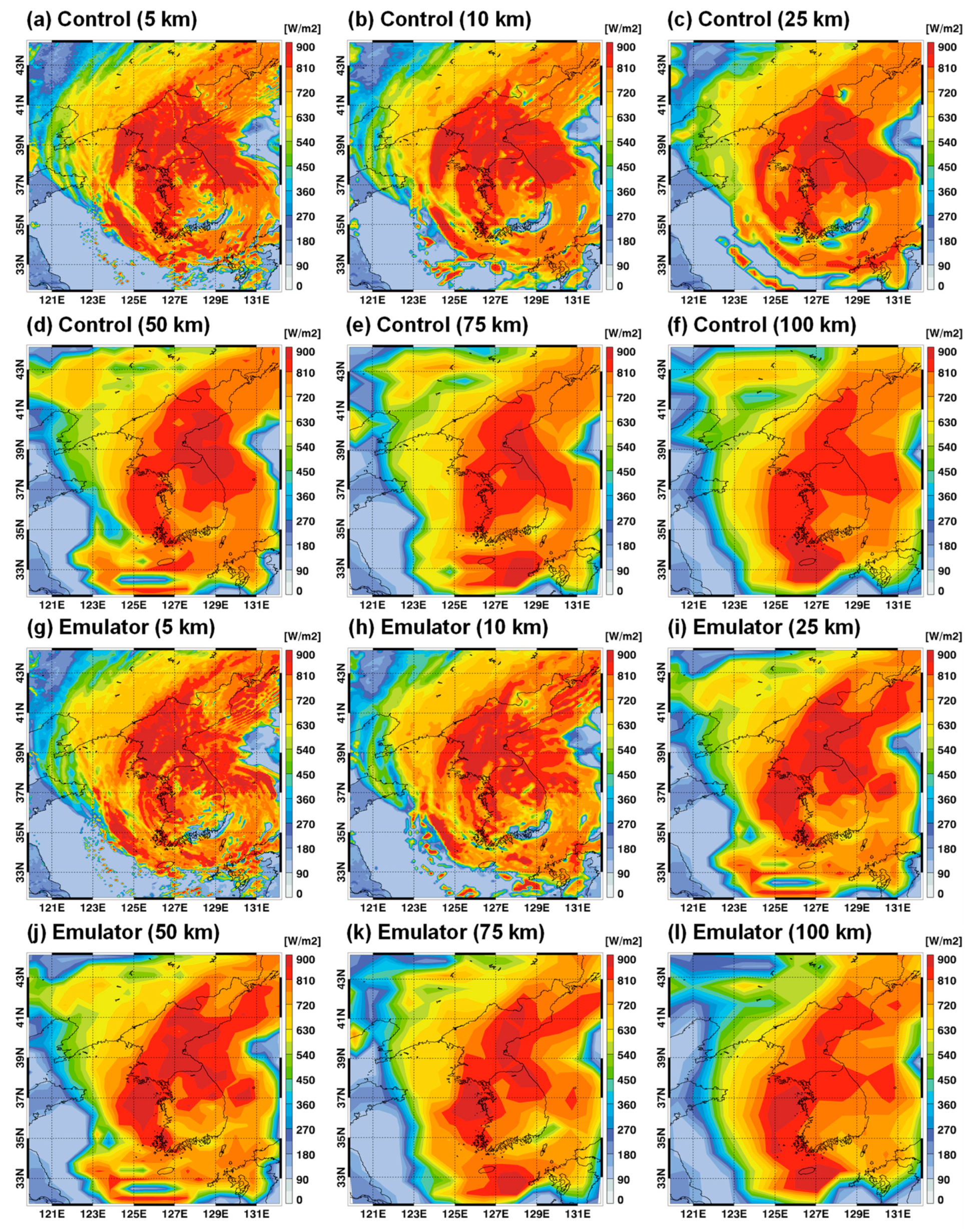
3.1. Real-Case Simulations

The forecast accuracy of the radiation emulator in the NWP model can be evaluated by comparing it with control simulations based on the original radiative transfer parameterization or observation data. To evaluate the accuracy of the LW/SW fluxes using a radiation emulator, we used the framework used by [19,20]. This framework considered 48 weekly cases (approximately one year) with a 3 h interval for 234 × 282 grids (5 km); thus, the statistics were obtained from 177,375,744 data points. Because different domain sizes, such as 118 × 142 (10 km), 48 × 57 (25 km), 25 × 29 (50 km), 16 × 20 (75 km), and 13 × 15 (100 km), were considered for resolution experiments, the number of data points were inversely proportional to horizontal resolution. The emulator results at different resolutions were compared with each control simulation. T2m and 3-hourly accumulated precipitation simulated using the radiation emulator and RRTMG-K were also compared with surface observation data for the 48 weekly cases.
Figure 2 illustrates the spatial distributions of RMSEs for all-sky LW/SW fluxes when the radiation emulator developed at a 5 km resolution was applied to 10–100 km resolutions. The WRF simulation results based on the Lambert conformal conic projection were interpolated to the latitude-longitude projection with a regular grid interval to draw the plots. First, the RMSEs of the LW flux showed a clear contrast between the land and ocean because the skin temperature and surface emissivity, as inputs for the LW radiation process, were separated for land and ocean. Note that the surface emissivity (LW) and albedo (SW) over the ocean are constant. Furthermore, mountainous areas can represent a strong variability in skin temperature toward colder temperatures than the surrounding low-latitude areas. Because the KLAPS model uses a terrain-following vertical coordinate, vertical profiles (e.g., pressure, temperature, and moisture) around the surface are affected by topographic altitudes. Therefore, the LW flux shows the largest error above 11 W m−2 in the Gaema Plateau area in North Korea, having the highest topographic altitude (Figure 2a). For the RMSEs of the SW flux, the land–ocean contrast was unclear; it increases slightly toward the southern region (Figure 2g). The more abundant cloud conditions and slightly larger insolation in the southern region explain the error pattern of SW flux. In contrast, in the Chinese desert areas located in the northwest, the lowest RMSEs for SW flux were found because of the low-cloud condition. As the horizontal resolutions become coarse horizontal resolutions to 10, 25, 50, 75, and 100 km, the RMSEs in both LW and SW decreased sharply. Because the radiation emulator used in this study was trained at 5 km resolution, the results at different resolutions should produce outputs with greater uncertainty regarding representation error. Nonetheless, the smoothing effects on the spatial input and output variables contributed to producing more accurate results in terms of universal application. Additionally, it provided lower representation errors in the observation at different resolutions. The lower representation error could be due to large training sets for the small Korean domain. The number of training sets used by [2,19] was 720 times larger than those used by [14,15,17]. Because the GCM domain covers the entire globe, using more training sets is essential to ensure universality and accuracy, as [19] used. Therefore, we can conclude that the 5 km simulation results of [2,18,19,20,21] were developed under more difficult conditions to secure the universality of radiation emulators compared with those at the 25 km resolution [15] and coarse resolutions larger than 100 km [10,11,12,13,14,15,16,17]. Similarly, we expect that developing a radiation emulator at resolutions less than 5 km, such as at the 0.25 km resolution [1], would be more difficult. Although this study did not consider real-case simulations at resolutions less than 5 km because of the limitation of computational resources, this issue is addressed in the ideal-case simulation framework.
Figure 3 and Figure 4 show a case example (03UTC 7 September 2020) of outgoing longwave radiation (OLR) and outgoing shortwave radiation (OSR) distributions between RRTMG-K control and emulator results. It corresponds to the 156 h forecast initialized from 15UTC 31 August 2020. This case exhibited a widely spread cloud pattern due to the influence of typhoon HAISEN. The lower OLR and higher OSR values indicate deep convective clouds and thick clouds, respectively. In contrast, higher OLR and lower OSR values are found in clear regions. The emulator results represented OLR and OSR distributions similar to those of the control simulations, although slight differences were observed because the accurate forecast of clouds is difficult. When the horizontal resolutions decreased from 5 km to 100 km, the simulated OLR and OSR patterns also varied significantly. However, judging from the similarity between control and emulator results, this change did not appear to have severely impacted the universal applicability of the radiation emulator.
For a more quantitative evaluation, the temporal variations in RMSEs for LW/SW fluxes, T2m, and 3-hourly accumulated precipitation were analyzed (Figure 5). The results obtained were for 48 weekly cases and the entire spatial domain. The RMSEs of the LW flux increased steadily with forecast time while showing diurnal variations (Figure 5a). Because the variability in surface temperature is larger during the daytime, the RMSEs of the LW flux showed an amplified error during the day. The RMSEs of the SW flux were characterized by a strong diurnal variation associated with the evident diurnal cycle of insolation while showing a gradual increase in error with forecast time (Figure 5b). In both LW and SW fluxes, the RMSEs at coarse resolutions were lower than those at fine resolutions. For resolutions larger than 50 km, the RMSE patterns in the LW flux were saturated (Figure 5a); similar trends were observed for the time series of RMSEs (Figure 5d–f). The total RMSEs for the three LW and SW fluxes are listed in Table 2. The RMSEs of the LW and SW fluxes for 5, 10, 25, 50, 75, and 100 km were 9.59, 9.16, 8.16, 7.79, 7.78, and 7.99 W m−2 and 63.17, 60.34, 52.78, 49.03, 46.89, and 47.40 W m−2, respectively. Accordingly, the 5 km results were more uncertain by 20% (LW) and 33% (SW) compared with the 100 km results. If the results would have been re-trained at each resolution, not aiming at the universal application of the 5 km radiation emulator, the difference between the 5 km and 100 km results would have been reduced. These results show that the 5 km simulations in [2,18,19,20,21] were harsher conditions than coarse resolutions larger than 100 km [10,11,12,13,14,15,16,17]. Compared with the observation data, the evaluation results revealed the contrast between T2m and precipitation (Figure 5c,d). The RMSEs of T2m increased with increasing resolution (2.2619 K to 2.9405 K in Table 2), whereas an opposite trend was observed for the 3-hourly precipitation (1.5515 mm to 1.1479 mm in Table 2). The control simulations based on the original radiation parameterization also exhibited similar RMSEs for T2m (2.2643 K to 2.9895 K) and 3-hourly precipitation (1.1433 mm to 1.5641 mm) (Table 2), as well as similar temporal evolutions (Figure 5e,f), compared to the emulator results. No significant performance degradation of the emulator results was observed compared to the control simulation results. When the horizontal resolution is coarse, the spatial variability of the simulated surface temperature can be less than that of the actual observations. Thus, overly coarse resolutions can degrade the forecast accuracy of the surface temperature. [30,31] reported similar results, showing lower accuracy for the surface temperature at coarse resolutions. Because the precipitation forecast is highly uncertain, the smoothing effect at coarse resolutions can be more important in determining the forecast error. Precipitation forecasting skill in numerical models was somewhat improved on coarse horizontal scales [28,29]. However, precipitation forecasts at fine resolutions are still important.
Notably, the mean bias was much smaller than the RMSE (Table 2), especially for the LW/SW fluxes. The systematic biases for LW/SW fluxes and precipitation increased as the horizontal resolution increased, contrary to the RMSEs. Furthermore, because the role of cumulus parameterization in determining precipitation and surface temperature is more important at coarse resolutions than at fine resolutions, we examined the behavior of radiation emulator results with a turned-off cumulus scheme. By disabling the cumulus scheme, the RMSEs for the LW/SW fluxes and T2m (listed in Table 2) were changed by a maximum of 0.9% (at 100 km resolution), while the general trends remained unchanged. The RMSEs of the 3-hourly precipitation forecasts at 100 km resolution were changed the most (by 6.7%), resulting in 0.2472 mm. Nevertheless, these results did not affect the conclusion of this study regarding the universal application of a radiation emulator at different resolutions. Therefore, the radiation emulator developed at 5 km resolution can be universally applied for horizontal resolutions larger than 5 km while maintaining accuracy and stability. However, the opposite situation (coarse to fine resolutions) cannot be guaranteed because the potential error from the radiation emulator can lead to unstable results in numerical models [13,17,18,20]. This drawback led to the next analysis based on ideal-case simulations.

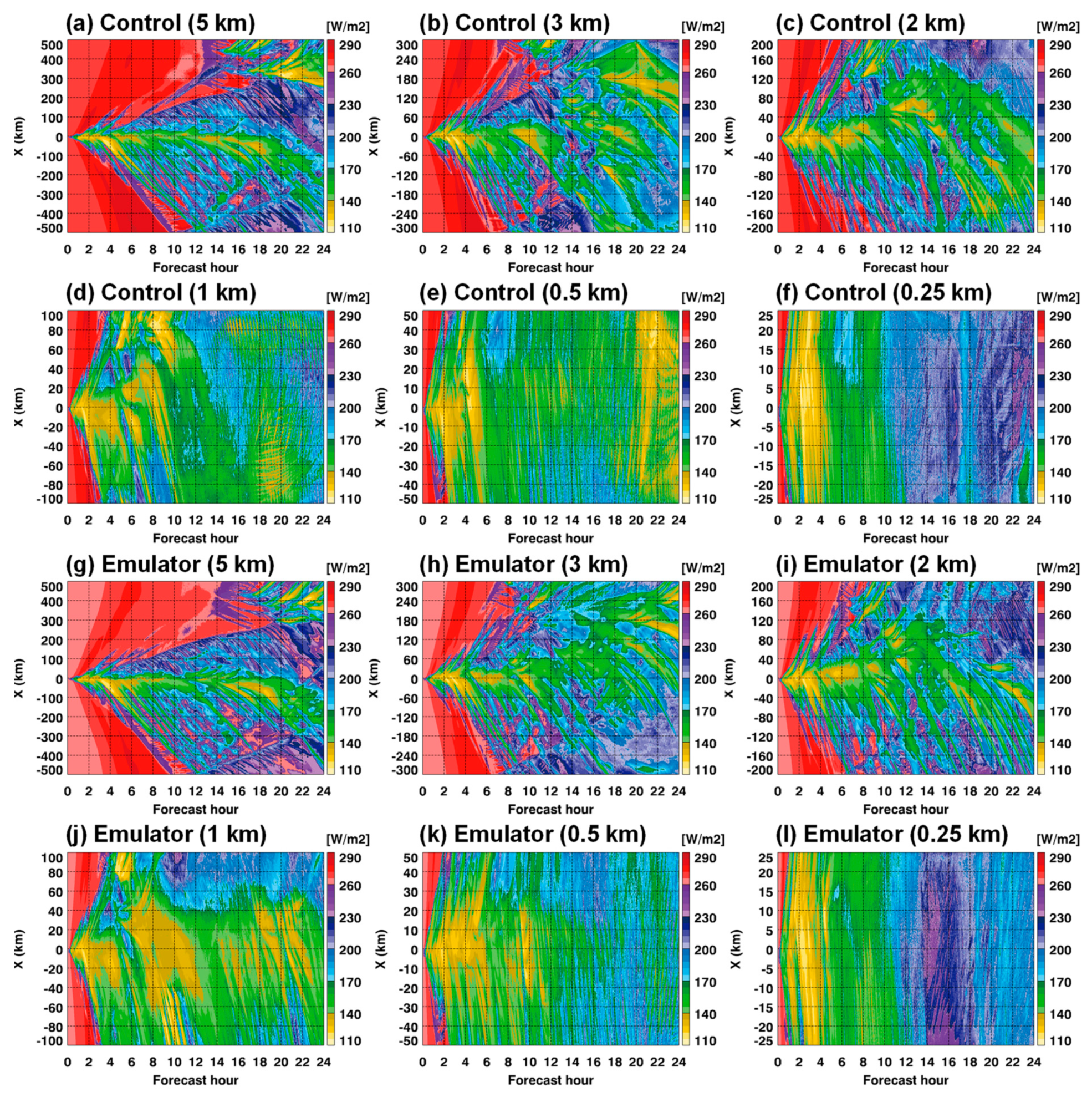
3.2. Ideal-Case Simulations

Considering a tremendous computation resource for long-term simulations at fine resolutions of less than 5 km, the universal application of a radiation emulator at 5–0.25 km resolutions was evaluated in a two-dimensional idealized squall line simulation as an extreme precipitating case. Similar ideal simulations were conducted by [1,19,20]. Ref. [20] examined the universal application of a radiation emulator with changes in 14 additional microphysics schemes at 5 km resolution. As a follow-up, our study examined the effects of horizontal resolution on a universal radiation emulator. The radiation emulator used in this study was considered for real-case simulation (July and land). This study considered a 24 h integral period with a 3 s time step; hence, the emulator was applied four times more than in the study by [1] for a 6 h forecast and 6.66 times more than in the study by [19,20] using a 20 s time step. The 3 s time step was essential for the control simulation at 0.25 km (larger time steps led to a blow-up of the control simulation). Comparing the representation error of the real-case simulation to that of the ideal-case, the RMSEs of the radiation emulator in [20] were greater by 24–48% than the infrequent use of radiative transfer parameterization by 60-fold in [19]. Because an ideal simulation is an extreme case, the error caused by the emulator can be rapidly amplified. Consequently, the RMSEs of the radiation emulator in Table 3 appear moderately large. These RMSEs were calculated for 201 horizontal grids and 1440 temporal data points at 10 min intervals. The heating rate and flux in this study represent the average of 39 vertical layers and 3 flux components (top and bottom), respectively. To minimize the error associated with universal representation, Ref. [20] attempted compound parameterization (CP [12]) returning to the original RRTMG-K parameterization when the predicted heating rate errors exceeded a predefined threshold. For the CP, an additional NN was trained using the same input variables in the emulator and the mean difference of vertical heating rates between the RRTMG-K and the emulator (i.e., one output variable), as well as the same 90 neurons and single hidden layer with the emulator. Although frequent CP can ensure the accuracy and stability of the radiation emulator, it can lead to a substantial slowdown toward the RRTMG-K parameterization, diminishing the fundamental value of the radiation emulator. Thus, considering the trade-off between accuracy and speed, using an appropriate threshold for activating the CP procedure is essential. Ref. [20] used thresholds of 1.0341 and 0.4820 K day−1 for the LW and SW heating rates, respectively, to target an approximately 3-fold slowdown of the emulator with a 60-fold speedup. If the predicted heating rate errors were less than those thresholds, the emulator mode with a 60-fold speedup was maintained. When the same concept was applied in this study, the emulator + CP results were 3.23–4.21 times slower than those obtained using the emulator alone. This result implies that the emulator + CP was 14–19 times faster than the original radiative transfer parameterization. By adding CP, the total RMSEs at 5 km resolution were reduced by 27.3%, 26.7%, 16.8%, and 16.8% for the LW heating rate, SW heating rate, LW flux, and SW flux, respectively. The resulting RMSEs of heating rates (2.61 K day−1 and 1.21 K day−1) were comparable to 2.57 K day−1 and 1.20 K day−1 based on the infrequent use of radiative transfer parameterization by 30 times [19]. In particular, systematic bias was reduced by the use of CP (Table 3). These results indicate that using a radiation emulator with CP can maintain stable accuracy while overcoming the representation error induced by the difference between the real and ideal cases and different horizontal resolutions.
Figure 6 shows the temporal and spatial variations of OLR (upward LW flux at the top of the atmosphere) for 5, 3, 2, 1, 0.5, and 0.25 km resolutions. Each simulation had the same horizontal grids but different coverage areas from 1000 km to 50 km. The difference in area coverage induced different evolutionary patterns among the control simulations. A low OLR indicates vigorous deep convention, whereas a high OLR represents a clear condition. While the 5 km control simulation is characterized by widely spread clear areas (expressed by high OLR values) before hour 12 (Figure 6a), the clear sky portion is rapidly reduced when the horizontal resolution decreases from 5 to 0.25 km. Because the radiative transfer error is larger in cloud profiles, the 0.25 km simulation corresponds to a more highly nonlinear situation than the 5 km simulation. The sharp effect at a fine resolution with more extreme events (in contrast to the smoothing effect at a coarse resolution) provides a more uncertain situation at 0.25 km resolution. Therefore, the occurrence frequencies of lower OLRs, regarded as deep convective clouds, are higher at fine resolutions in both real and ideal cases (Figure 7). In contrast to the long-term (one year) results for the real case showing a stable smoothing effect with resolution (Figure 7a), the ideal simulations based on one case show great variability in probability density functions (Figure 7b). Because of the sharp effect and the high cloud conditions at fine resolutions, the occurrence frequencies of OLRs less than 180 W m−2 were higher at fine resolutions, whereas those around 270 W m−2, regarded as a clear condition, were relatively reduced. Characteristically, the 0.25 km simulation showed a rare occurrence with OLRs of less than 180 W m−2. In contrast, it showed frequent occurrences of OLRs between 180 and 220 W m−2, compared with those at other fine resolutions (2 km, 1 km, and 0.5 km). As shown in blue in Figure 6f, the 0.25 km simulation produced medium OLRs of 180–220 W m−2 after 12-h. This results from nonlinear characteristics in the cloud-resolving simulation.
With these control simulation characteristics, the radiation emulators (with CP) successfully reproduced features similar to those of the control simulations until 24 h (Figure 6g–i). The ideal simulation was sensitive to small initial perturbations and rapidly changed during integration. The clear area in the initial stage at coarse resolutions and the subsequent widely spread clouds were realistically expressed in the emulator results, despite the results being trained from real-case simulations. The difference between control and emulator results was larger at fine resolutions. For example, OLRs higher than 200 W m−2 after 20 h in the control simulation at 0.25 km were not found in the 0.25 km emulator result. Figure 8 illustrates the vertical RMSEs of the heating rates and the temporal RMSEs of the fluxes. The RMSEs were calculated for the temporal–horizontal grids and horizontal grids, respectively. The 1 km and 0.5 km simulations showed a larger error in the middle-level heating rates (Figure 8a,b). A large error also characterized the 0.5 km simulation in the LW heating rate around the surface (Figure 8a). For the LW flux, no characteristic features were observed at a specific resolution (Figure 8c). The RMSE of the SW flux was the largest in the 0.25 km simulation, especially around 15–16 h. In contrast, the RMSEs for 1 km and 0.5 km simulations were characteristically lower than those for coarse resolutions (Figure 8d).
Because the ideal simulation is a highly nonlinear process, a consistent tendency with resolutions, such as in the real case, was not found. Increasing errors at fine resolutions using an emulator were evident. Compared with the 5 km simulation, for the 0.25–3 km resolutions, the errors of the LW heating rate, SW heating rate, LW flux, and SW flux increased by 19–128%, 41–104%, 6–96%, and 17–57%, respectively (Table 3). The increase in these errors as a function of horizontal resolutions was higher than that induced by microphysics parameterization changes, which were at 5 km resolution in [20]. When using CP, the RMSE increases with resolution changes were reduced to 13–72% and 9–45% in LW and SW heating rates, respectively, compared with those at the 5 km resolution. For LW and SW fluxes, the RMSE increases were improved by a maximum of 5% and 8%, respectively, at coarse resolutions. Although the RMSEs were higher at fine resolutions than at coarse resolutions, this study is not the blow-up issue of the entire model, such as the unphysical OLR in [17]. Therefore, we can conclude that the radiation emulator developed at 5 km resolution can be universally applied for cloud-resolving resolutions less than 5 km while maintaining accuracy at the expense of computational speed by using CP (i.e., 60-fold to 14–19-fold speedup). Furthermore, when the overall statistics were reanalyzed with the same spatial domain of ±0.25 km, the conclusion of this study did not change significantly (Table 4). Because cloud areas were dominant over ±0.25 km (Figure 6), the RMSEs at coarse resolutions were mostly increased, while the use of CP was not.

4. Conclusions

In this study, we considered different horizontal resolutions under two simulation frameworks: KLAPS over the Korean peninsula (real case) and two-dimensional squall line simulation (ideal case) to examine the impact of horizontal resolution on the universal applicability of the radiation emulator in NWP models. The real-case simulation was performed for approximately one year with a 7-day forecast time, whereas the ideal-case simulation was an extreme squall line case with a 1-day forecast time. Horizontal resolutions were 5, 10, 25, 50, 75, and 100 km (convection-permitting scale to climate simulation scale) for the real-case simulation and 5, 3, 2, 1, 0.5, and 0.25 km (convection-permitting scale to cloud-resolving scale) for the ideal-case simulations. All emulator simulations were based on the NN radiation scheme developed under the real case at 5 km simulations by [19]. This emulator was 60-fold faster than the RRTMG-K radiative transfer parameterization. In our study, all simulations were tested in an independent period (i.e., 2020), while the emulator was trained for 2009–2019. The real-case simulation focused only on the impact of horizontal resolutions on the universal applicability of the 5 km radiation emulator. In contrast, the ideal-case simulation further considered the universal robustness arising from the difference between the real and ideal cases. Despite the different horizontal resolutions with the trained 5 km resolution, the forecast error of the LW/SW fluxes was significantly reduced from fine to coarse resolutions (9.59 to 7.79 W m−2 and 63.17 to 46.89 W m−2). In addition, the RMSEs of T2m and precipitation, compared with the observations, increased and decreased from fine to coarse resolutions (2.2619 K to 2.9405 K and 1.5515 mm to 1.1479 mm, respectively). Because control simulations also showed the same error characteristic for T2m, these results suggested that the radiation emulator developed at a 5 km resolution universally applies to horizontal resolutions larger than 5 km while maintaining accuracy and stability. For the ideal-case simulation, the temporal and spatial evolutions of the OLRs were examined for different horizontal resolutions (5, 3, 2, 1, 0.5, and 0.25 km). Each control simulation showed a large difference in the temporal and spatial cloud patterns due to the smoothing effect at coarse resolutions and different cloud conditions. Using a radiation emulator successfully reproduces features similar to the control simulations. For 0.25–3 km resolutions, the forecast errors of the LW heating rate, SW heating rate, LW flux, and SW flux increased by 19–128%, 41–104%, 11–123%, and 17–57%, respectively, compared with those for the 5 km simulation. To minimize these errors, the CP that was 3.23–4.21 times slower than the emulator was further used (the emulator + CP was 14–19 times faster than the original radiative transfer parameterization). By adding CP, the total RMSEs at 5 km resolution were reduced by 27.3%, 26.7%, 22.3%, and 16.8% for the LW heating rate, SW heating rate, LW flux, and SW flux, respectively. The resulting RMSEs of LW heating rate, SW heating rate, LW flux, and SW flux at 5–0.25 km resolutions were 2.61 to 4.49 K day−1, 1.21 to 1.75 K day−1, 15.60 to 17.65 W m−2, and 101.52 to 174.04 W m−2, respectively. Here, the resulting RMSEs of heating rates at 5 km resolution (2.61 and 1.21 K day−1) were comparable to 2.57 and 1.20 K day−1 based on the infrequent use of original radiative transfer parameterization by 30 times [19].
This study provides a comprehensive overview of radiation emulator studies using numerical prediction models at different resolutions. This study found that the evaluated error of the emulator with coarse-resolution modeling was reduced compared to the control run. Therefore, previous emulator studies on convection-permitting and cloud-resolving scales were regarded as more valuable than those on low-resolution based on climate models. In addition, these results provide important information on the universal applicability of radiation emulators associated with the use of different horizontal resolutions and modeling platforms. Although the universal robustness of the radiation emulator has been examined for changes in numerical models and microphysics parameterization [17,20], no experiments at a different resolution from the trained resolution have been conducted. The efforts in this study are variable, as this study is the first to show the universal applicability of radiation emulators at different resolutions. Therefore, this study can form the basis for the complete replacement of radiative transfer parameterization by a machine-learning emulator with a significant speedup. This study can also accelerate the computational speed of regional climate simulations or high-resolution modeling regarding a faster radiation scheme. The findings in this study also suggest an evident direction for developing the universal radiation emulator in the future that should be developed at the highest possible resolution. When applied to high-resolution models, the emulator trained at low resolution had great uncertainty because the occurrence frequency of extreme events was underestimated in the low-resolution modeling. For universal application, the training sets can be increased to encompass global regions (as against this study which was confined to the Korean peninsula).

Author Contributions

H.-J.S.: conceptualization, data curation, formal analysis, investigation, methodology, software, validation, visualization, and writing—original draft and writing. S.R.: writing—review and editing. All authors gave final approval for publication and agreed to be held accountable for the work performed therein. All authors have read and agreed to the published version of the manuscript.

Funding

H.-J. Song gratefully acknowledges financial support by the Korea Meteorological Administration (KMA) Research and Development Program “Developing AI technology for weather forecasting” under Grant (KMA2021-00121) and by the National Research Foundation of Korea (NRF) grant funded by the Korea government (MSIT) (RS-2023-00210362). Additionally, S. Roh was supported by the National Research Foundation of Korea (NRF) grant funded by the Korea government (MSIT) (RS-2023-00211994).

Data Availability Statement

The neural network radiation scheme, real and ideal-case modeling system used in this study was obtained from Song et al., (2022) [19]. The data and codes used in this manuscript are available in the following: https://doi.org/10.5281/zenodo.5638436. Although both systems were based on the WRF model (version 3.9.1.1), they were modified to use the radiation emulator.

Conflicts of Interest

The authors declare no known competing financial interests or personal relationships that could have appeared to influence the work reported in this paper.

References

  1. Roh, S.; Song, H.-J. Evaluation of neural network emulations for radiation parameterization in cloud resolving model. Geophys. Res. Lett. 2020, 47, e2020GL089444. [Google Scholar] [CrossRef]
  2. Song, H.-J.; Roh, S. Improved weather forecasting using neural network emulation for radiation parameterization. J. Adv. Model. Earth Syst. 2021, 13, e2021MS002609. [Google Scholar] [CrossRef]
  3. Chevallier, F.; Chéruy, F.; Scott, N.A.; Chédin, A. A neural network approach for a fast and accurate computation of a longwave radiative budget. J. Appl. Meteorol. 1998, 37, 1385–1397. [Google Scholar] [CrossRef]
  4. Liu, Y.; Caballero, R.; Monteiro, J.M. RadNet 1.0: Exploring deep learning architectures for longwave radiative transfer. Geosci. Model Dev. 2020, 13, 4399–4412. [Google Scholar] [CrossRef]
  5. Ukkonen, P.; Pincus, R.; Hogan, R.J.; Nielsen, K.P.; Kaas, E. Accelerating radiation computations for dynamical models with targeted machine learning and code optimization. J. Adv. Model. Earth Syst. 2020, 12, e2020MS002226. [Google Scholar] [CrossRef]
  6. Lagerquist, R.; Turner, D.; Ebert-Uphoff, I.; Stewart, J.; Hagerty, V. Using deep learning to emulate and accelerate a radiative transfer model. J. Atmos. Ocean. Technol. 2021, 38, 1673–1696. [Google Scholar] [CrossRef]
  7. Veerman, M.A.; Pincus, R.; Stoffer, R.; van Leeuwen, C.M.; Podareanu, D.; van Heerwaarden, C.C. Predicting atmospheric optical properties for radiative transfer computations using neural networks. Philos. Trans. R. Soc. A 2021, 379, 20200095. [Google Scholar] [CrossRef]
  8. Meyer, D.; Hogan, R.J.; Dueben, P.D.; Mason, S.L. Machine learning emulation of 3D cloud radiative effects. J. Adv. Model. Earth Syst. 2022, 14, e2021MS002550. [Google Scholar] [CrossRef]
  9. Ukkonen, P. Exploring pathways to more accurate machine learning emulation of atmospheric radiative transfer. J. Adv. Model. Earth Syst. 2022, 14, e2021MS002875. [Google Scholar] [CrossRef]
  10. Belochitski, A.; Binev, P.; DeVore, R.; Fox-Rabinovitz, M.; Krasnopolsky, V.; Lamby, P. Tree approximation of the long wave radiation parameterization in the NCAR CAM global climate model. J. Comput. Appl. Math. 2011, 236, 447–460. [Google Scholar] [CrossRef]
  11. Krasnopolsky, V.M.; Fox-Rabinovitz, M.S.; Chalikov, D.V. New approach to calculation of atmospheric model physics: Accurate and fast neural network emulation of longwave radiation in a climate model. Mon. Weather Rev. 2005, 133, 1370–1383. [Google Scholar] [CrossRef]
  12. Krasnopolsky, V.M.; Fox-Rabinovitz, M.S.; Belochitski, A.A. Decadal climate simulations using accurate and fast neural network emulation of full, longwave and shortwave radiation. Mon. Weather Rev. 2008, 136, 3683–3695. [Google Scholar] [CrossRef]
  13. Krasnopolsky, V.M.; Fox-Rabinovitz, M.S.; Tolman, H.L.; Belochitski, A.A. Neural network approach for robust and fast calculation of physical processes in numerical environmental models: Compound parameterization with a quality control of larger errors. Neural Netw. 2008, 21, 535–543. [Google Scholar] [CrossRef]
  14. Krasnopolsky, V.M.; Fox-Rabinovitz, M.S.; Hou, Y.T.; Lord, S.J.; Belochitski, A.A. Accurate and fast neural network emulations of model radiation for the NCEP coupled Climate Forecast System: Climate simulations and seasonal predictions. Mon. Weather Rev. 2010, 138, 1822–1842. [Google Scholar] [CrossRef]
  15. Krasnopolsky, V.M.; Belochitski, A.A.; Hou, Y.T.; Lord, S.J.; Yang, F. Accurate and Fast Neural Network Emulations of Long and Short Wave Radiation for the NCEP Global Forecast System Model. NCEP/NWS, NOAA, Office Note 471. 2012. Available online: https://www.emc.ncep.noaa.gov/officenotes/newernotes/on471.pdf (accessed on 1 May 2012).
  16. Pal, A.; Mahajan, S.; Norman, M.R. Using deep neural networks as cost-effective surrogate models for Super-Parameterized E3SM radiative transfer. Geophys. Res. Lett. 2019, 46, 6069–6079. [Google Scholar] [CrossRef]
  17. Belochitski, A.; Krasnopolsky, V. Robustness of neural network emulations of radiative transfer parameterizations in a state-of-the-art General Circulation Model. Geosci. Model Dev. 2021, 14, 7425–7437. [Google Scholar] [CrossRef]
  18. Song, H.-J.; Roh, S.; Park, H. Compound parameterization to improve the accuracy of radiation emulator in a numerical weather prediction model. Geophys. Res. Lett. 2021, 48, e2021GL095043. [Google Scholar] [CrossRef]
  19. Song, H.-J.; Roh, S.; Lee, J.; Nam, G.; Yun, E.; Yoon, J.; Kim, P.S. Benefits of stochastic weight averaging in developing neural network radiation scheme for numerical weather prediction. J. Adv. Model. Earth Syst. 2022, 14, e2021MS002921. [Google Scholar] [CrossRef]
  20. Song, H.-J.; Kim, P.S. Effects of cloud microphysics on the universal performance of neural network radiation scheme. Geophys. Res. Lett. 2022, 49, e2022GL098601. [Google Scholar] [CrossRef]
  21. Kim, P.S.; Song, H.-J. Usefulness of automatic hyperparameter optimization in developing radiation emulators in a numerical weather prediction model. Atmosphere 2022, 13, 721. [Google Scholar] [CrossRef]
  22. Morcrette, J.-J. Radiation and cloud radiative properties in the European Centre for Medium Range Weather Forecasts forecasting system. J. Geophys. Res. 1991, 96, 9121. [Google Scholar] [CrossRef]
  23. Iacono, M.J.; Delamere, J.S.; Mlawer, E.J.; Shephard, M.W.; Clough, S.A.; Collins, W.D. Radiative forcing by long-lived greenhouse gases: Calculations with the AER radiative transfer models. J. Geophys. Res. 2008, 113, D13103. [Google Scholar] [CrossRef]
  24. Baek, S. A revised radiation package of G-packed McICA and two-stream approximation: Performance evaluation in a global weather forecasting model. J. Adv. Model. Earth Syst. 2017, 9, 1628–1640. [Google Scholar] [CrossRef]
  25. Hogan, R.J.; Bozzo, A. A flexible and efficient radiation scheme for the ECMWF model. J. Adv. Model. Earth Syst. 2018, 10, 1990–2008. [Google Scholar] [CrossRef]
  26. Pincus, R.; Mlawer, E.J.; Delamere, J.S. Balancing accuracy, efficiency, and flexibility in radiation calculations for dynamical models. J. Adv. Model. Earth Syst. 2019, 11, 3087–3089. [Google Scholar] [CrossRef] [PubMed]
  27. Shin, H.-C.; Ha, J.-H.; Ahn, K.D.; Lee, E.H.; Kim, C.H.; Lee, Y.H.; Clayton, A. An overview of KMA’s operational NWP data assimilation system. In Data Assimilation for Atmospheric, Oceanic and Hydrologic Applications (Vol. IV); Park, S.K., Xu, L., Eds.; Springer: Cham, Switzerland, 2022. [Google Scholar] [CrossRef]
  28. Roberts, N.M.; Lean, H.W. Scale-selective verification of rainfall accumulations from high-resolution forecasts of convective events. Mon. Weather Rev. 2008, 136, 78–97. [Google Scholar] [CrossRef]
  29. Clark, P.; Roberts, N.; Lean, H.; Ballard, S.P.; Charlton-Perez, C. Convection-permitting models: A step-change in rainfall forecasting. Meteorol. Appl. 2016, 23, 165–181. [Google Scholar] [CrossRef]
  30. Pavlik, D.; Söhl, D.; Pluntke, T.; Mykhnovych, A.; Bernhofer, C. Dynamic downscaling of global climate projections for eastern Europe with a horizontal resolution of 7 km. Environ. Earth Sci. 2012, 65, 1475–1482. [Google Scholar] [CrossRef]
  31. Kumar, P.; Ojha, S.P.; Singh, R.; Kishtawal, C.M.; Pal, P.K. Performance of weather research and forecasting model with variable horizontal resolution. Theor. Appl. Climatol. 2016, 126, 705–713. [Google Scholar] [CrossRef]
  32. Morrison, H.; Thompson, G.; Tatarskii, V. Impact of cloud microphysics on the development of trailing stratiform precipitation in a simulated squall line: Comparison of one- and two-moment schemes. Mon. Weather Rev. 2009, 137, 991–1007. [Google Scholar] [CrossRef]
  33. Lim, K.S.; Hong, S.-Y. Development of an effective double-moment cloud microphysics scheme with prognostic cloud condensation nuclei (CCN) for weather and climate models. Mon. Weather Rev. 2010, 138, 1587–1612. [Google Scholar] [CrossRef]
  34. Morrison, H.; Milbrandt, J.A. Parameterization of cloud microphysics based on the prediction of bulk ice particle properties. Part I: Scheme description and idealized tests. J. Atmos. Sci. 2015, 72, 287–311. [Google Scholar] [CrossRef]
  35. Bae, S.Y.; Hong, S.-Y.; Tao, W.-K. Development of a single-moment cloud microphysics scheme with prognostic hail for the Weather Research and Forecasting (WRF) model. Asia-Pac. J. Atmos. Sci. 2019, 55, 233–245. [Google Scholar] [CrossRef]
  36. Izmailov, P.; Podoprikhin, D.; Garipov, T.; Vetrov, D.; Wilson, A.G. Averaging weights leads to wider optima and better generalization. arXiv 2018, arXiv:1803.05407. [Google Scholar] [CrossRef]
  37. Skamarock, W.C.; Klemp, J.B.; Dudhia, J.; Gill, D.O.; Liu, Z.; Berner, J.; Wang, W.; Powers, J.G.; Duda, M.G.; Barker, D.M.; et al. A Description of the Advanced Research WRF Model Version 4; NCAR Technical Notes; NCAR: Boulder, CO, USA, 2019. [Google Scholar] [CrossRef]
  38. Kwon, Y.C.; Hong, S. A mass-flux cumulus parameterization scheme across gray-zone resolutions. Mon. Weather Rev. 2017, 145, 583–598. [Google Scholar] [CrossRef]
  39. Shin, H.H.; Hong, S. Representation of the subgrid-scale turbulent transport in convective boundary layers at gray-zone resolutions. Mon. Weather Rev. 2015, 143, 250–271. [Google Scholar] [CrossRef]
  40. Jiménez, P.A.; Dudhia, J.; González-Rouco, J.F.; Navarro, J.; Montávez, J.P.; García-Bustamante, E. A revised scheme for the WRF surface layer formulation. Mon. Weather Rev. 2012, 140, 898–918. [Google Scholar] [CrossRef]
  41. Hersbach, H.; Bell, B.; Berrisford, P.; Hirahara, S.; Horányi, A.; Muñoz-Sabater, J.; Nicolas, J.; Peubey, C.; Radu, R.; Schepers, D.; et al. The ERA5 global reanalysis. Q. J. R. Meteorol. Soc. 2020, 146, 1999–2049. [Google Scholar] [CrossRef]
  42. Zhong, X.; Ma, Z.; Yao, Y.; Xu, L.; Wu, Y.; Wang, Z. WRF–ML v1.0: A bridge between WRF v4.3 and machine learning parameterizations and its application to atmospheric radiative transfer. Geosci. Model Dev. 2023, 16, 199–209. [Google Scholar] [CrossRef]
Figure 1. Locations of surface 713 stations (red circles) used for 2 m temperature and precipitation observations, along with background topography (gray colors).
Remotesensing 15 02637 g001
Figure 2. Spatial distributions of RMSEs for LW and SW fluxes compared to the control runs with different horizontal resolutions in real-case simulations. The area marked with a black circle in (a) represents the Gaema Plateau.
Remotesensing 15 02637 g002
Figure 3. Spatial distributions of outgoing longwave radiation (OLR) for a typhoon case (03UTC 7 September 2020) between (af) control runs and (gl) emulator simulations with different horizontal resolutions. Because it is 6.5-day forecast result, the radiation emulator was applied 28,080 times with a 20 s time step.
Remotesensing 15 02637 g003
Figure 4. Same as Figure 3, but for outgoing shortwave radiation (OSR).
Remotesensing 15 02637 g004
Figure 5. Time series of RMSEs for (a) LW and (b) SW fluxes compared to the control runs with different horizontal resolutions in real-case simulations. The observational evaluations of 2 m temperature (T2m) and 3-hourly precipitation were given for both (c,d) emulator (e,f) and control simulations.
Remotesensing 15 02637 g005
Figure 6. Spatial-temporal evolutions of outgoing longwave radiation (OLR) with different horizontal resolutions between control runs and emulator results in ideal-case simulations.
Remotesensing 15 02637 g006
Figure 7. Probability density functions (PDF) of outgoing longwave radiation (OLR) between (a) real-case and (b) ideal-case simulations at different horizontal resolutions.
Remotesensing 15 02637 g007
Figure 8. Vertical RMSEs of (a) LW and (b) SW heating rates, as well as temporal RMSEs of (c) LW and (d) SW fluxes, compared to the control runs with different horizontal resolutions in ideal-case simulations. The results were derived from 1 min interval data over the entire domain.
Remotesensing 15 02637 g008
Table 1. Comparison of offline evaluations (i.e., for independent validation sets) for all-sky LW heating rate (LWHR) and SW heating rate (SWHR) profiles in the literature and this study. The root mean square errors (RMSEs) for LWHR and SWHR were given. All results were based on the fully connected feed-forward neural network, except Ukkonen (2022) [9] used the recurrent neural network and Zhong et al. (2023) [42] using bidirectional long short-term memory (Bi-LSTM).
ReferencesResolution
[km]
Speedup
[Fold]
LWHR
[K day−1]
SWHR
[K day−1]
Krasnopolsky et al. (2010) [14]3001000.340.19
Krasnopolsky et al. (2010) [14]100300.490.20
Krasnopolsky et al. (2012) [15]25400.520.26
Roh and Song (2020) [1]0.25301.120.55
Roh and Song (2020) [1]0.25601.541.13
Roh and Song (2020) [1]0.251001.601.15
Song and Roh (2021) [2]5600.590.22
Ukkonen (2022) [9]804-0.16
Song et al. (2022) [19]5600.460.18
Zhong et al. (2023) [42]515.712.0351.172
Zhong et al. (2023), Bi-LSTM [42]52.160.3370.277
Table 2. Total root mean square error (RMSE) statistics and mean bias (in parenthesis) for real-case simulations by using a radiation emulator. The LW and SW fluxes [W m−2], along with three upward (↑) and downward (↓) fluxes at the top and bottom, were compared with the control model simulations, whereas 2-m temperature (T2m) [K] and 3-hourly precipitation [mm] were compared with surface observations. The observational evaluations for control simulations were also given in the bottom panel.
5 km10 km25 km50 km75 km100 km
LW flux9.5888
(−0.0896)
9.1575
(−0.1974)
8.1587
(−0.3312)
7.7853
(−0.4591)
7.7776
(−0.5351)
7.9902
(−0.5777)
-top ↑11.2884
(−0.1130)
10.6651
(−0.4161)
9.2559
(−0.8553)
8.8752
(−1.3604)
9.2227
(−1.7208)
9.8026
(−1.9578)
-bottom ↑3.8179
(−0.0127)
3.7173
(0.0041)
3.4111
(0.0326)
3.3648
(0.1044)
3.2523
(0.1382)
3.3526
(0.1812)
-bottom ↓13.6601
(−0.1430)
13.0901
(−0.1801)
11.8089
(−0.1709)
11.1159
(−0.1214)
10.8579
(−0.0227)
10.8154
(0.0436)
SW flux63.1709
(0.5536)
60.3422
(0.6708)
52.7777
(0.8328)
49.0250
(1.1012)
46.8944
(1.2480)
47.3956
(1.4263)
-top ↑79.3886
(−0.2232)
75.9043
(−0.8143)
62.3987
(−1.6583)
61.6078
(−2.9714)
58.9609
(−3.3387)
59.6203
(−3.9874)
-bottom ↑13.6354
(0.1701)
12.9018
(0.2718)
11.3199
(0.4041)
10.4635
(0.6312)
10.0865
(0.7353)
10.0846
(0.8843)
-bottom ↓96.4886
(1.7138)
92.2204
(2.5550)
80.6146
(3.7526)
75.0035
(5.6438)
71.6357
(6.3475)
72.4819
(7.3819)
T2m2.2619
(−0.7778)
2.4536
(−0.9370)
2.6596
(−0.9582)
2.7026
(−0.7280)
2.8249
(−0.6236)
2.9405
(−0.5037)
Precipitation1.5515
(−0.0703)
1.5170
(−0.0846)
1.3788
(−0.1426)
1.2800
(−0.2136)
1.1747
(−0.2965)
1.1479
(−0.3393)
T2m (Control)2.2643
(−0.7791)
2.4607
(−0.9428)
2.6808
(−0.9733)
2.7401
(−0.7726)
2.8672
(−0.6775)
2.9895
(−0.5656)
Precipitation
(Control)
1.5641
(−0.0629)
1.5123
(−0.0890)
1.3775
(−0.1444)
1.2760
(−0.2187)
1.1776
(−0.2981)
1.1433
(−0.3435)
Table 3. Total root mean square error (RMSE) and mean bias (in parenthesis) statistics for ideal-case simulations. The LW and SW heating rates [K day−1] and the LW and SW fluxes [W m−2] were compared with the control simulations. The numbers before and after arrows ( ) indicate the emulator only and the emulator with compound parameterization.
LW Heating RateSW Heating RateLW FluxSW Flux
5 km3.59 2.61
(−0.05 −0.11)
1.65 1.21
(0.30 0.02)
25.12 20.89
(0.36 0.12)
193.19 160.76
(12.97 1.84)
3 km4.42 2.96
(0.14 −0.07)
2.48 1.64
(0.64 0.02)
36.01 20.35
(10.18 −1.83)
260.52 154.19
(47.00 −1.81)
2 km4.29 2.98
(0.13 −0.17)
2.32 1.33
(0.52 0.01)
26.67 21.92
(0.74 1.10)
225.13 147.67
(15.56 −2.12)
1 km5.19 3.87
(−0.25 −0.41)
3.37 1.75
(1.33 −0.13)
39.41 20.29
(17.71 −0.91)
291.27 104.46
(99.03 11.92)
0.5 km5.90 4.49
(−0.21 −0.40)
3.30 1.75
(1.39 −0.06)
49.14 19.73
(26.86 3.11)
269.50 101.52
(89.70 2.24)
0.25 km5.29 3.44
(−0.35 0.01)
2.99 1.43
(1.10 0.00)
45.06 19.73
(24.96 −3.47)
245.47 174.04
(61.15 5.32)
Table 4. Same as Table 3, but for statistics over the same ±25 km domain.
LW Heating RateSW Heating RateLW FluxSW Flux
5 km4.39 2.44
(0.02 −0.09)
2.19 1.28
(0.66 0.01)
23.62 15.08
(−1.50 −0.27)
244.51 88.27
(30.11 −2.80)
3 km4.77 2.91
(0.12 −0.11)
2.29 1.09
(0.77 0.02)
36.38 15.87
(11.77 −2.35)
262.38 93.95
(55.03 −1.65)
2 km5.15 2.99
(0.22 −0.16)
2.52 1.03
(0.63 0.004)
23.67 18.07
(−0.99 0.59)
225.38 81.35
(18.20 1.35)
1 km5.33 4.00
(−0.22 −0.44)
3.33 1.66
(1.33 −0.21)
34.40 18.30
(11.99 −5.64)
301.92 66.41
(95.43 20.50)
0.5 km6.00 4.52
(−0.20 −0.37)
3.38 2.18
(1.38 −0.04)
49.87 19.64
(26.43 2.40)
292.46 109.32
(86.37 1.39)
0.25 km5.29 3.44
(−0.35 0.006)
2.99 1.43
(1.10 0.002)
45.06 19.73
(24.96 −3.47)
245.47 174.04
(61.15 5.32)
Disclaimer/Publisher’s Note: The statements, opinions and data contained in all publications are solely those of the individual author(s) and contributor(s) and not of MDPI and/or the editor(s). MDPI and/or the editor(s) disclaim responsibility for any injury to people or property resulting from any ideas, methods, instructions or products referred to in the content.

