Article

Tropospheric Second-Order Horizontal Gradient Modeling for GNSS PPP

GNSS Research Center, Wuhan University, 129 Luoyu Road, Wuhan 430079, China
*
Author to whom correspondence should be addressed.
Remote Sens. 2022, 14(19), 4807; https://doi.org/10.3390/rs14194807
Submission received: 8 September 2022 / Revised: 22 September 2022 / Accepted: 23 September 2022 / Published: 26 September 2022
(This article belongs to the Special Issue Beidou/GNSS Precise Positioning and Atmospheric Modeling II)

Abstract

:
The asymmetric delay has a considerable impact on Global Navigation Satellite Systems (GNSS) Positioning, Navigation and Timing (PNT) applications. In GNSS analyses, the impacts of the asymmetric delay are commonly compensated by using the classical methods with considering the north-south and east-west horizontal gradients. In this paper, we have initiatively proposed an extended method where the north-south and east-west horizontal gradients as well as the second-order horizontal gradients are included to better fit the asymmetric delay. The modeling accuracy of the extended method was evaluated at globally distributed 905 GNSS stations during 40 days in 2020. Significant performance of the extended method respect to the classical method was found, where the hydrostatic and wet modeling accuracy at 4° elevation angle was improved from 5.3 and 10.6 mm to 1.6 and 4.9 mm by 70% and 54%, respectively. The GNSS Precise Point Positioning (PPP) performance using the extended method was also validated at 107 Multi-GNSS Experiment (MGEX) stations. The superior performance on the coordinate repeatability and significant effectiveness on the coordinate and Zenith Total Delay (ZTD) estimations were also found, and the maximal vertical (U) coordinate and ZTD difference biases reached 8.6 and −4.5 mm. The extended method is therefore recommended to substitute the classical methods in the GNSS analyses, especially under severe atmospheric conditions.

Graphical Abstract

1. Introduction

The electromagnetic wave signals of Global Navigation Satellite Systems (GNSS) are inevitably delayed and bent during their passage through the neutral atmosphere, generating the tropospheric Slant Total Delay (STD) that can be written as [1,2,3,4,5]:
S T D ( e , α ) = Z H D · M F h ( e ) + Z W D · M F w ( e ) isotropic   part + M F g ( e ) · ( G n · cos ( α ) + G e · sin ( α ) ) anisotropic   part
where e and α denote elevation angle and azimuth. Z H D and Z W D represent for Zenith Hydrostatic and Wet Delay. M F h , M F w and M F g stand for hydrostatic, wet and gradient mapping functions. G n and G e are the two horizontal gradient components in north-south and east-west directions.
The tropospheric delay can be divided into isotropic and anisotropic delays according to the azimuthal variation characteristics. The isotropic part is the product of Zenith Path Delay (ZPD) and mapping function that has been well discussed in the existing literature [6,7,8,9,10]. The anisotropic part is usually expressed as the function of north-south and east-west gradients based on the assumption of the tilting atmosphere, deriving the frequently used classical methods such as TANZ, CHENHER, and TILTING [11,12,13]. The classical methods are suitable for the asymmetry delays from the thermal expansion of the earth’s atmosphere and the distribution of the atmospheric water vapor on macroscale, while they are degraded under severe topographic perturbation or extreme weather situations, mainly due to the constraint of the simple sine and cosine structure [2].
To overcome this issue, the classical methods were extended. Gegout et al. [14] designed the Adaptive Mapping Function (AMF) based on the mapping function continued fraction and the CHENHER method, using tens of parameters to fit thousands of symmetric and asymmetric delays simultaneously, and the fitting accuracy reaches millimeter level. Masoumi et al. [15] proposed a directional model on the basis of the CHENHER method where the omni-direction is divided into several discrete azimuthal wedges and the asymmetry in each wedge is approximated independently, and the superior performance was found both in asymmetry modeling and Global Positioning System (GPS) Precise Point Positioning (PPP) under extreme weather scenarios. Landskron and Böhm [2] developed the Extended CHENHER (ECHENHER) method where the number of parameters is increased from 2 to 4, and significant improvement was also found for the modeling at low elevation angle and the Very Long Baseline Interferometry (VLBI) analyses.
However, up to now, the extended methods are all derived from the CHENHER method and focus on asymmetric modeling, lack of researches based on the more rigorous TILTING method and on the impacts of GNSS parameter estimation. In this paper, we will initiatively introduce an extended method named Extended TILTING (ETILTING) based on the ECHENHER and TILTING methods, and then systematically compare the asymmetry modeling and GNSS PPP performance of the ETILTING method. This paper is organized as follows: Section 2 describes the TANZ, CHENHER, TILTING, ECHENHER and ETILTING methods. Section 3 evaluates the asymmetry modeling performance of different methods. Section 4 compares the GNSS PPP performance by using the five modeling methods. Section 5 summarizes the work and conclusions.

2. Asymmetric Delay Modeling Methods

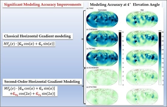
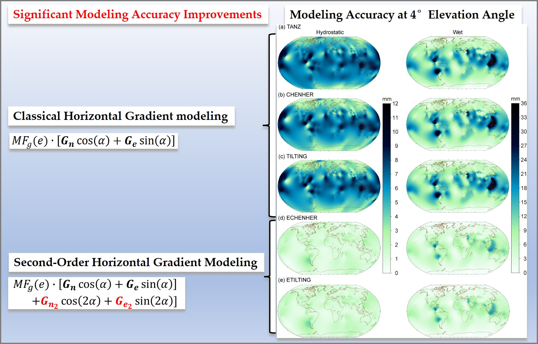
2.1. Classical Methods

The classical methods are all based on the tilting atmosphere assumption, and the different methods are mainly distinguished by their gradient mapping functions. MacMillan [11] proposed the TANZ method to compensate for the asymmetric effects on VLBI observations where the gradient mapping function is expressed by the product of the mapping function and 1 / tan ( e ) as:
A D ( e , α ) = M F ( e ) tan ( e ) · [ G n cos ( α ) + G e sin ( α ) ]
where A D denotes the Asymmetric Delay (AD). M F is the mapping function and takes M F h , M F w and M F w for the hydrostatic, wet and total asymmetry modeling, respectively. Two years later, Chen and Herring [12] proposed the widely-used CHENHER method as:
A D ( e , α ) = 1 sin ( e ) · tan ( e ) + C · [ G n cos ( α ) + G e sin ( α ) ]
where C represents the gradient mapping function constant, and it takes values of 0.0031, 0.0007 and 0.0032 for the hydrostatic, wet and total asymmetry modeling, respectively. In addition, Meindl et al. [13] derived the TILTING method using the assumption of tilting zenith direction where the gradient mapping function is the derivation of M F respect to e as:
A D ( e , α ) = d M F d e · [ G n cos ( α ) + G e sin ( α ) ]
where d M F d e is the gradient mapping function, and it takes the values of d M F h d e , d M F w d e and d M F w d e for the hydrostatic, wet, and total modeling, respectively.

2.2. Extended Methods

The extended methods proposed by Gegout et al. [14] and Masoumi et al. [15] are too complicated to apply in operational modeling and positioning applications, and therefore only the ECHENHER and ETILTING methods will be described in this section. Landskron and Böhm [2] considered the higher-order variation of asymmetric delay and added the second-order horizontal gradients to the standard gradient formula of the CHENHER method (Equation (3)), deriving the ECHENHER method as:
A D ( e , α ) = 1 sin ( e ) · tan ( e ) + C · [ G n cos ( α ) + G e sin ( α ) + G n 2 cos ( 2 α ) + G e 2 sin ( 2 α ) ]
where G n 2 and G e 2 are the second-order horizontal gradient parameters. In this paper, we introduce the ETILTING method on the basis of the TILTING and ECHENHER methods as:
A D ( e , α ) = d M F d e · [ G n cos ( α ) + G e sin ( α ) + G n 2 cos ( 2 α ) + G e 2 sin ( 2 α ) ]
where d M F d e denotes the gradient mapping function that can change with the atmosphere state, and it is the main advantage of the ETILTING method over the ECHENHER method. The characteristics of the extended methods are compared with the classical methods in Table 1.

3. Modeling Evaluations

3.1. Modeling Strategies

We use the ray-tracing technique to retrieve hourly Slant Hydrostatic Delay (SHD) and Slant Wet Delay (SWD) from reanalysis products [16,17]. In this work, the fifth-generation Re-Analysis (ERA5) products from the European Centre for Medium-Range Weather Forecasts (ECMWF) were selected for the ray-tracing calculations [18,19], considering the superior temporal-spatial resolutions (1 h, 0.25° and 37 pressure levels) and performance [20]. The Slant Path Delays (SPDs) included SHD and SWD were retrieved at 14 elevation angles (3°, 4°, 5°, 6°, 7°, 8°, 10°, 12°, 15°, 20°, 30°, 50°, 70°, and 80°) and 16 azimuths (with an interval of 22.5°) [1,2], spanning four seasons (11–20 January, 11–20 April, 11–20 July, and 11–20 October in 2020) and covering 905 globally distributed stations as shown in Figure 1, including 549 International GNSS Service (IGS) stations and 356 stations in China.
We used the classical (TANZ, CHENHER and TILTING) and extended (ECHENHER and ETILTING) methods to model the asymmetry component of SPDs. Firstly, the asymmetric delays at 7 elevation angles (3°, 5°, 7°, 10°, 15°, 30° and 70°) and 16 azimuths (with an interval of 22.5°) were calculated by subtracting the SPD average from the SPDs at 16 azimuths [1]. Then, the modeling was performed by taking the calculated asymmetric delays as inputs and using the least-squares method where the hydrostatic and wet asymmetric delays are modeled separately with equal weighting [1]. Finally, the five corresponding horizontal gradient models spanning 40 days and covering 905 stations were derived.

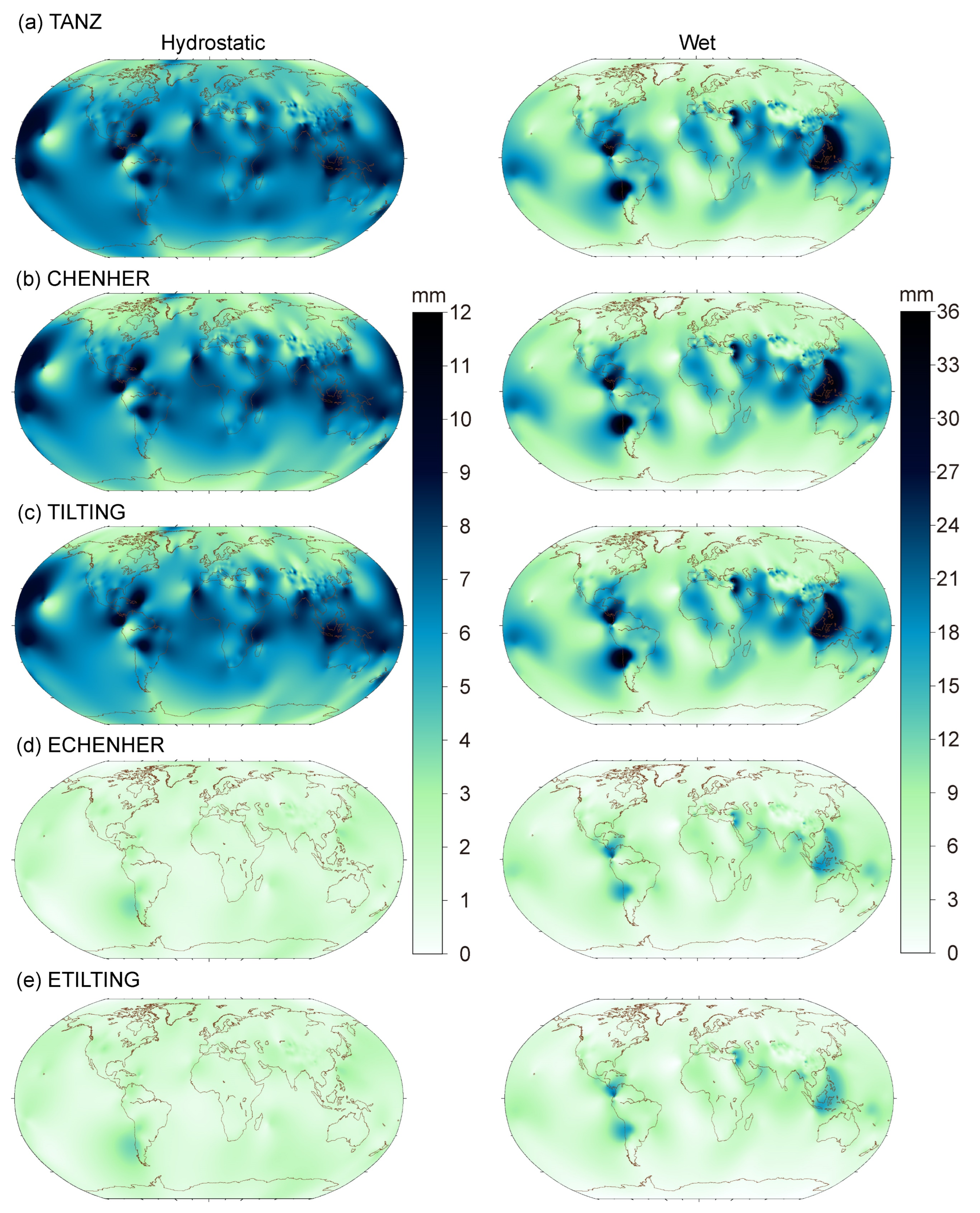
3.2. Modeling Residual Evaluations

In this section, we evaluate the modeling residuals using the five methods. For the evaluations, the precision index, Mean Absolute Error (MAE), was adopted [1,2,21]. The MAE at a specific elevation angle and azimuth can be calculated as:
M A E ( e , α ) = | A D o ( e , α ) A D c ( e , α ) |
where A D o denotes the ray-traced asymmetric delay, and A D c represents the asymmetric delay calculated from the horizontal gradient models. In this evaluation, the residual MAEs at the input modeling elevation angles and azimuths were first computed over 40 days and 905 stations. Then, the statistically residual MAEs at different modeling elevation angles were retrieved by taking the average of the MAEs at all the input azimuths and stations in 964 epochs (hours during a 40-day period) and shown in Table 2. We can find that, in the three classical methods, the TANZ method, generally with the largest residual MAEs, is obviously worst both for the hydrostatic and wet component modeling, while the CHENHER and TILTING methods show the best performance for hydrostatic and wet modeling, respectively. Compared with the classical methods, the extended methods show significant improvements at the low elevation angles (≤10°) and slight degradation at the high elevation angles. The reason is that the asymmetric delays at different elevation angles are equally weighted in the modeling, and the second-order horizontal gradient estimations slightly contaminate the modeling at high elevation angles.
As shown in Table 2, the residual MAEs at 3° elevation angle are generally the largest, and, therefore, we further present the residual MAE distribution for the 905 stations at 3° elevation angle in Figure 2, where the hydrostatic and wet MAE distributions have different color bars. We can find that the MAE distribution for the three classical methods is similar (Figure 2a–c). The hydrostatic MAE distribution has latitude and topography dependence where the middle and low latitude stations around the ocean and mountains show larger MAEs, mainly due to the effects of more active atmospheric states and more severe atmospheric perturbations [22]. Compared with the hydrostatic MAE distribution, the wet MAE distribution also shows latitude and topography dependence. Several middle and low-latitude coastal areas, such as the north coast of South America, the west coast of South America, the east coast of the Mediterranean Sea, and the east of Southeast Asia, present large MAEs, indicating the deficiencies of the classical methods. Compared with the classical methods, the extended methods show significant improvements both in MAE distribution and magnitude (Figure 2d,e). For the hydrostatic component, the latitude and topography dependence almost disappear, and the MAE magnitudes also clearly decrease. As for the wet component, although the latitude and topography dependence still exist in several regions, such as the east coast of the Mediterranean Sea and the east of Southeast Asia, the MAE is obviously smaller compared to the classical methods.

3.3. Modeling Accuracy Evaluations

In this section, we evaluate the modeling accuracy of different horizontal gradient models at independent elevation angles that are not involved in the modeling (4°, 6°, 8°, 12°, 20°, 50° and 80°). We first calculated the MAEs at the 905 stations and 16 azimuths in 964 epochs, and then took the average MAEs at different elevation angles and showed the statistical results in Table 3. We can also find that the CHENHER and TILTING methods perform best for hydrostatic and wet modeling, respectively. The extended methods obviously have better performance both for the hydrostatic and wet components at low elevation angles, and the maximal improvement exceeds 6 mm. As for the two extended methods, the ECHENHER method is slightly better for hydrostatic modeling, and the ETILTING method has better wet modeling performance with a maximal improvement of about 0.62 mm.
The modeling MAEs using different methods are generally largest at 4° elevation angle, and the MAE distribution for the 905 stations is therefore presented at 4° elevation angle in Figure 3. We can find that the classical methods have similar MAE distributions (Figure 3a–c). The hydrostatic MAE distribution is correlated with the station latitudes, and the middle and low latitude areas with more active hydrostatic atmosphere states show larger MAEs [22]. In addition, the MAE distribution also depends on the topography to some degree, and some sea and land boundary areas show much larger MAEs. The wet MAE distribution also shows obvious latitude and topography dependence, and several coastal areas, such as the north and west coasts of South America and eastern areas of Southeast Asia, have much larger MAEs. In contrast, the MAE distribution of the extended methods is much better (Figure 3d,e), where latitude and topography dependence are not obvious anymore.

4. GNSS PPP Validations

4.1. Data Processing Strategies

In operational GNSS analyses, the effects of asymmetric delay are generally modeled by the north-south and east-west gradient estimations using the classical method. In this section, we initiatively use the extended method instead of the classical method for horizontal gradient estimations considering the better modeling accuracy and compare the multi-GNSS PPP performances of different methods. There are three classical methods (TANZ, CHENHER, and TILTING) and two extended methods (ECHENHER and ETILTING) involved in the GNSS analyses, where the classical methods estimate the G n and G e parameters, and the extended methods additionally include the two second-order horizontal gradient parameters ( G n 2 and G e 2 ). In addition, the multi-GNSS PPP with no horizontal estimations (NONE) is also performed. Therefore, a total of six PPP schemes will be included in this section.
We use the Positioning and Navigation Data Analyst (PANDA) software [23] to analyze the multi-GNSS (GPS+GLONASS+GALILEO+BDS3) data from 107 globally distributed IGS Multi-GNSS Experiment (MGEX) stations as shown in Figure 1 [24], and the time period is from 11–20 October in 2020. The satellite orbits are fixed by the German Research Center for Geosciences (GFZ) GBM products, and the satellite clock corrections are estimated every 5 min using the corresponding schemes to the PPP processing to avoid the influence of inconsistency. The detailed processing strategies for the six PPP schemes are listed in Table 4.

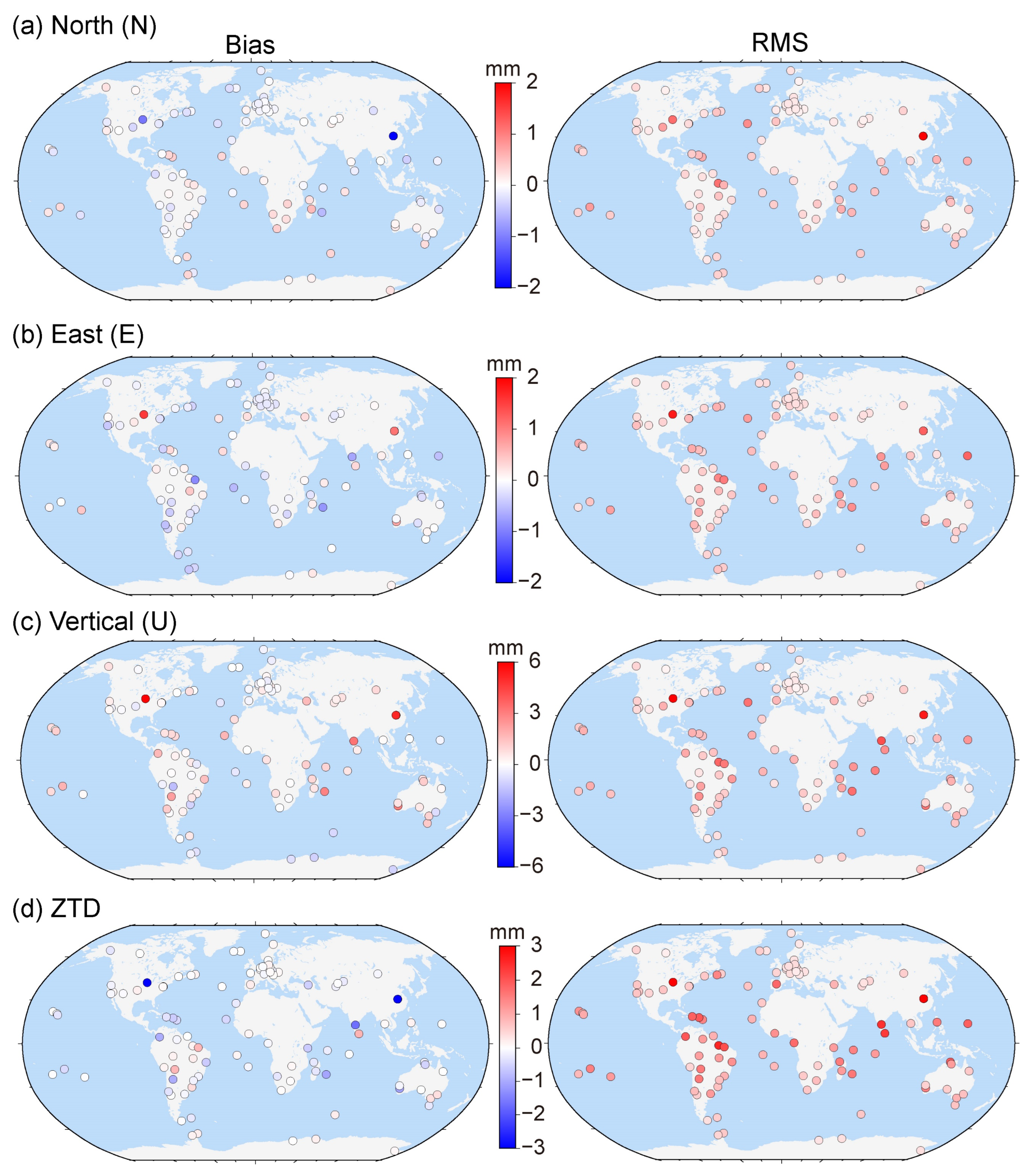
4.2. Coordinate Repeatability

In this section, we compare the coordinate repeatability of the six PPP schemes. We first extracted the 10-day coordinate time series from the PPP daily solutions and then removed the effect of Atmospheric Pressure Loading (APL) on the time series by using the APL products from Technische Universitat Wien [26,27]. After that, we calculated the coordinate repeatability without and with APL correction as shown in Table 5.
We can find that the APL correction improves the vertical (U) coordinate repeatability by about 0.3 mm with slightly contaminating the North (N) and East (E) components. The six PPP schemes have different performances in which the PPP scheme without gradient estimation (NONE) shows the worst repeatability, with a standard deviation of 1.84, 1.52 and 3.83 mm in the N, E and U directions, respectively. Compared with the NONE scheme, the schemes using the three classical methods show improvements reaching about 0.9, 0.6 and 0.7 mm on average. As for the extended methods, the coordinate repeatability is further improved by about 0.02, 0.05 and 0.05 mm, showing the advantages of estimating the second-order horizontal gradients. While for the schemes using different classical methods or extended methods, the coordinate repeatability is very close in which the TILTING and ETILTING schemes are slightly better than the CHENHER and ECHENER schemes. However, the coordinate repeatability differences between different schemes are not as significant as the modeling accuracy differences, and the main reason is that the modeling accuracy differences are concentrated on the low elevation angles, which are greatly suppressed by the elevation-dependent weighting strategy.
In addition to the statistical coordinate repeatability, the coordinate repeatability difference distribution between the TILTING and ECHENHER schemes and the ETILTING scheme is also shown in Figure 4, where the red color represents that the TILTING and ECHENHER schemes are worse than the ETILTING scheme. We can find that the coordinate repeatability differences between the TILTING and ETILTING schemes are obviously larger than those between the ECHENER and ETILTING schemes, demonstrating that the impact of the number of horizontal gradient parameters to be estimated is larger than the gradient mapping functions. In all 107 stations, there are 59, 69 and 60 stations with better N, E and U coordinate repeatability for the ETILTING scheme than for the TILTING scheme, again indicating the superior performance of the ETILTING method (left column of Figure 4). The U coordinate repeatability differences are most remarkable in the three coordinate components, and some middle and low latitude stations around the ocean show more significant differences with the maximal value of 2.32 mm (left column of Figure 4c) that is consistent with the modeling accuracy distribution.

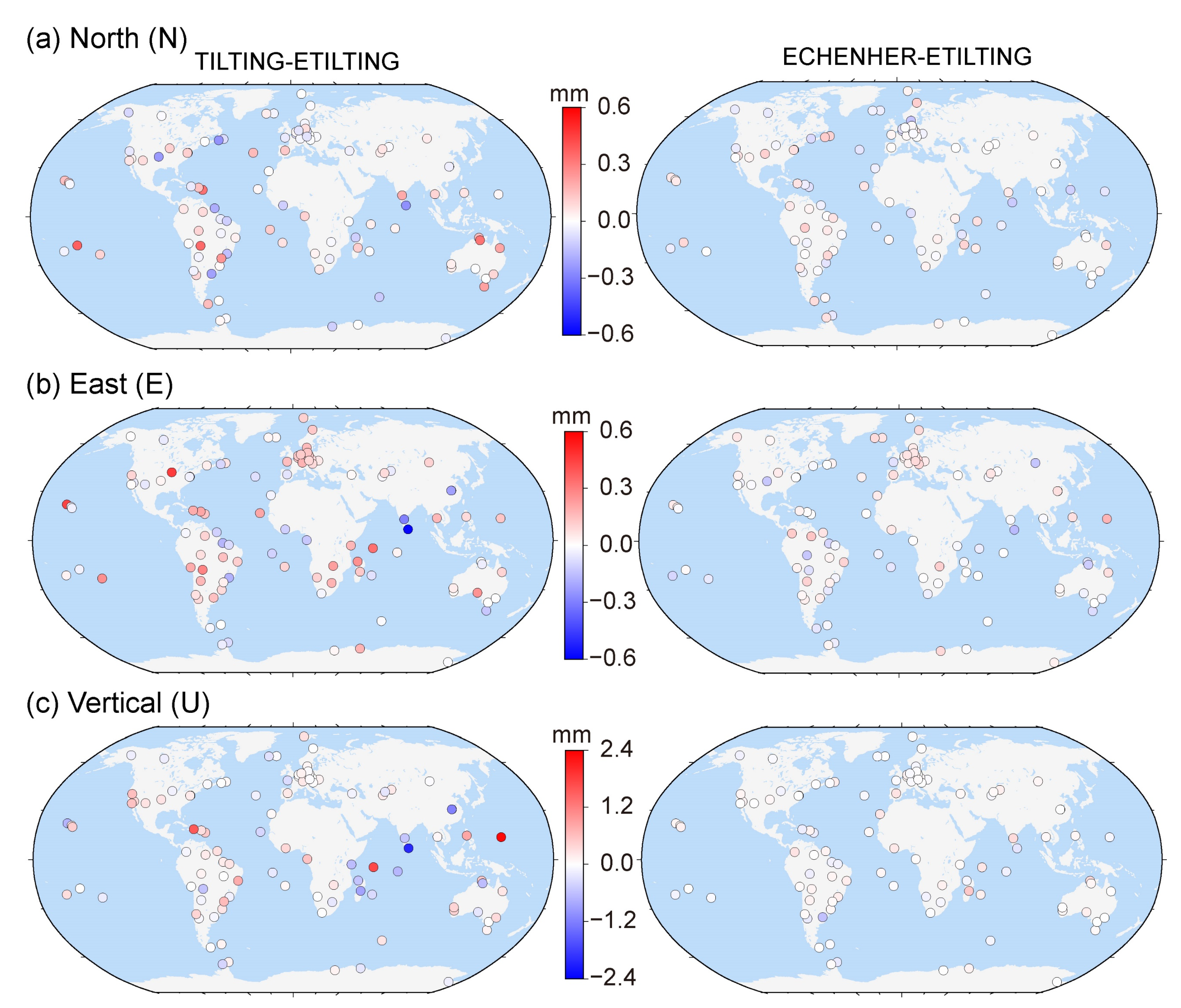
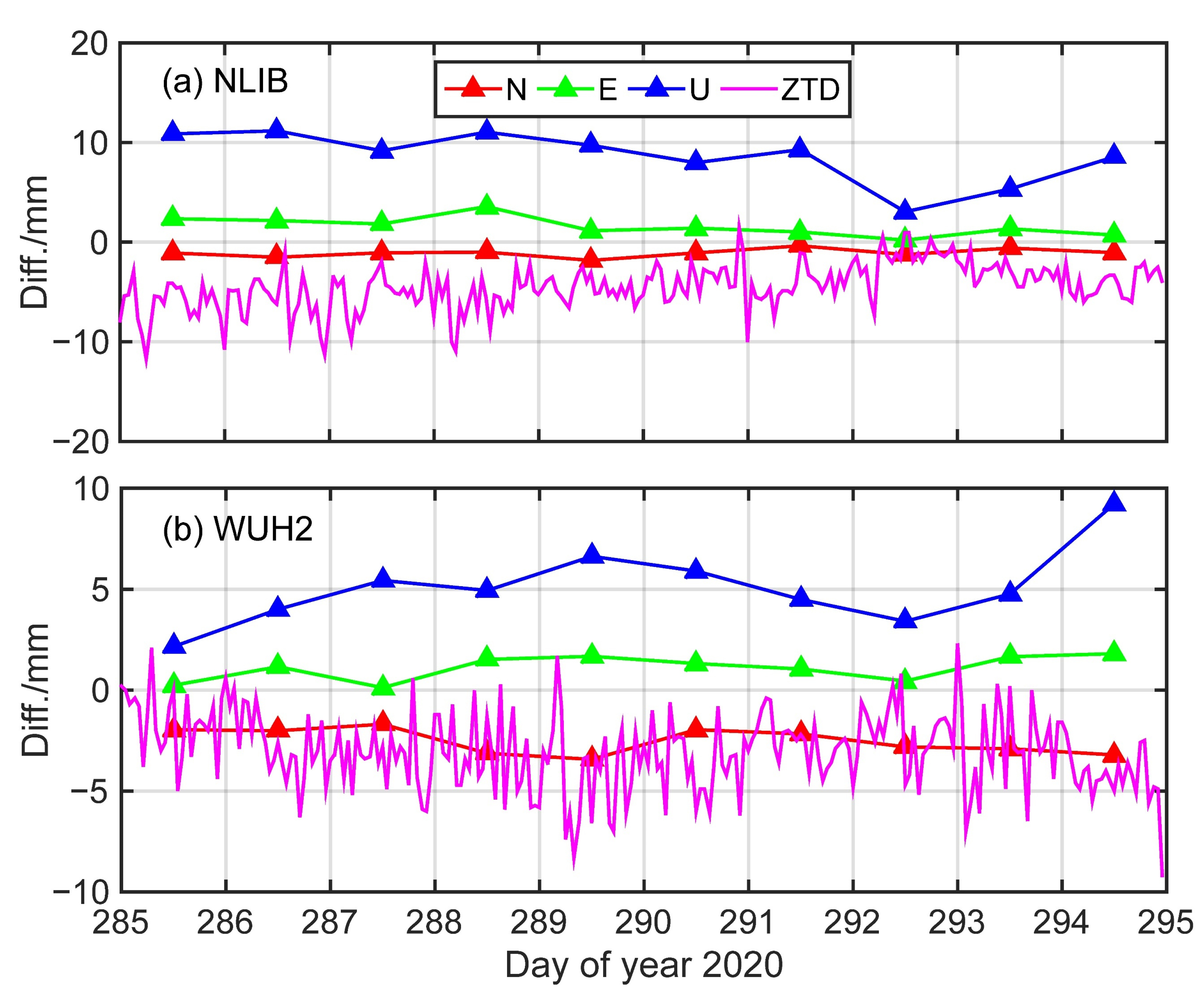
4.3. Coordinate and ZTD Differences

The coordinate repeatability cannot reflect the potential systematic bias in the position time series. Therefore, we further analyzed the coordinate and Zenith Total Delay (ZTD) differences between the TILTING, ECHENHER and TILTING schemes, where the statistical difference bias and Root Mean Square (RMS) are summarized in Table 6. We can find that the coordinate and ZTD differences between the TILTING and ETILTING schemes are also more significant than the differences between the ECHENHER and ETILTING schemes, illustrating the effectiveness of the second-order horizontal gradient estimation. Among all the statistical components, the U coordinate and ZTD differences are larger than the horizontal component differences, and the biases are 0.49 and −0.19 mm, respectively, indicating the potential systemic biases between the TILTING and ETILTING schemes.
In order to further illustrate the potential systematic bias, we plotted the bias and RMS distribution of the coordinate and ZTD differences between the TILTING and ETILTING schemes in Figure 5. We can find that the horizontal coordinate difference bias and RMS are smaller than the U coordinate and ZTD. The U coordinate difference biases have the opposite sign to ZTD, and the magnitudes are generally double those of the ZTD biases, indicating the strong correlation between U coordinate and ZTD [28]. The U coordinate and ZTD difference biases also depend on the station latitude, and the stations located in the middle and low latitudes generally show larger values, such as WUH2 (China) and NLIB (North America). At the two stations, the U coordinate and ZTD difference biases are nearly equal to the corresponding RMSs, indicating the significant systematic biases between the TILTING and ETILTING schemes. Considering the prominent biases, we further presented the coordinate and ZTD difference time series in Figure 6. We can find that the coordinate and ZTD difference time series between the two schemes are consistently positive or negative, with the statistical N, E, U, and ZTD difference biases of −1.08, 1.56, 8.61 and −4.47 mm for NLIB station, and of −2.53, 1.10, 5.10 and −3.02 mm for WUH2 station, demonstrating the significant effectiveness of the proposed ETILTING method relative to the TILTING method.

5. Conclusions

The asymmetric delays have non-negligible impacts on GNSS analyses. In the past decades, several classical methods, such as TANZ, CHENHER and TILTING, were proposed for better eliminating the impacts. However, limited by the simple sine and cosine structures, the classical methods perform poorly under the atmospheric state with severe variation. To deal with the issue, more sophisticated extended methods were introduced. In this paper, we reviewed the existing classical and extended methods and initiatively proposed a new extended method named ETILTING. The modeling residual and accuracy of the existing methods and the ETILTING method at 905 GNSS stations during 40 days in 2020 were evaluated. We found that the extended methods show very significant improvements to the classical methods both for the modeling residual and accuracy, where the hydrostatic and wet modeling accuracy of the ETILTING method at 4° elevation angle is improved from 5.3 and 10.6 mm of the TILTING method to 1.6 and 4.9 mm by 70% and 54%, respectively. As for the extended methods, the ETILTING method shows better performance than the ECHENHER method, and the maximal improvement in the modeling accuracy reaches 0.62 mm.
In addition, the multi-GNSS PPP performance of different methods was also validated at 107 MGEX stations. The coordinate repeatability as well as the coordinate and ZTD differences were systematically compared. The results show that the PPP scheme using the ETILTING method can improve the N, E, and U coordinates repeatability from 0.94, 0.94 and 3.11 mm to 0.92, 0.89 and 3.06 mm, indicating the superior performance of the ETILTING method to the TILTING method. In addition, the significant U coordinate and ZTD biases between the schemes using the TILTING and ETILTING methods were also found, and the maximum U coordinate and ZTD difference biases reached 8.6 and −4.5 mm, illustrating the effectiveness of the ETILTING method. In brief, the extended methods have better accuracy and PPP performance. We recommend the extended methods to substitute the frequently-used classical methods in the GNSS analyses, especially under severe atmospheric conditions.

Author Contributions

Conceptualization, Y.Z., Y.L. and W.Z.; methodology, Y.Z., W.Z. and Y.L.; software, Y.Z. and W.Z.; validation, Y.Z., W.Z. and Y.L.; formal analysis, Y.Z. and W.Z.; investigation, Y.Z. and W.Z.; resources, Y.Z., P.W., J.B. and Z.Z.; data curation, Y.Z., J.B. and Z.Z; writing—original draft preparation, Y.Z.; writing—review and editing, Y.L., W.Z. and Y.Z.; visualization, Y.Z.; supervision, Y.L. and W.Z.; project administration, Y.L. and W.Z.; funding acquisition, Y.L. and W.Z. All authors have read and agreed to the published version of the manuscript.

Funding

This work was supported by the National Natural Science Foundation of China (42174027); Key Research and Development Program of Guangxi Zhuang Autonomous Region, China (2020AB44004); the Fundamental Research Funds for the Central Universities (2042022kf1198).

Data Availability Statement

ERA5 was downloaded from Copernicus Climate Data Store (https://cds.climate.copernicus.eu/) (accessed on 7 September 2022). IGS MGEX RINEX data and GFZ GBM satellite orbit product are available through IGS CDDIS FTP (ftps://gdc.cddis.eosdis.nasa.gov/) (accessed on 7 September 2022) and GFZ FTP (ftp://ftp.gfz-potsdam.de/) (accessed on 7 September 2022). APL products was downloaded from Technische Universität Wien (http://vmf.geo.tuwien.ac.at/) (accessed on 7 September 2022).

Acknowledgments

Authors would like to thank Copernicus Climate Data Store, IGS CDDIS and GFZ for providing the research datasets and products, and acknowledge Technische Universität Wien for releasing APL products. The numerical calculations in this paper have been done on the supercomputing system in the Supercomputing Center of Wuhan University.

Conflicts of Interest

The authors declare no conflict of interest.

References

  1. Landskron, D. Modeling Tropospheric Delays for Space Geodetic Techniques. Doctoral Dissertation, Department of Geodesy and Geoinformation, TU Wien, Vienna, Austria, 2017. Supervisor: Böhm J. Available online: http://repositum.tuwien.ac.at/obvutwhs/content/titleinfo/2099559 (accessed on 7 September 2022).
  2. Landskron, D.; Böhm, J. Refined discrete and empirical horizontal gradients in VLBI analysis. J. Geod. 2018, 92, 1387–1399. [Google Scholar] [CrossRef]
  3. Liu, J.; Gao, K.; Guo, W.; Cui, J.; Guo, C. Role, path, and vision of “5G + BDS/GNSS”. Satell. Navig. 2020, 1, 23. [Google Scholar] [CrossRef]
  4. Huang, L.; Zhu, G.; Liu, L.; Chen, H.; Jiang, W. A global grid model for the correction of the vertical zenith total delay based on a sliding window algorithm. GPS Solut. 2021, 25, 98. [Google Scholar] [CrossRef]
  5. Huang, L.; Chen, H.; Liu, L.; Jiang, W. A new high-precision global model for calculating zenith tropospheric delay. Chin. J. Geophys.-CH 2021, 64, 782–795. [Google Scholar] [CrossRef]
  6. Zhu, G.; Huang, L.; Liu, L.; Li, C.; Li, J.; Huang, L.; Zhou, L.; He, H. A new approach for the development of grid models calculating tropospheric key parameters over China. Remote Sens. 2021, 13, 3546. [Google Scholar] [CrossRef]
  7. Huang, L.; Zhu, G.; Peng, H.; Chen, H.; Liu, L.; Jiang, W. A global grid model for the vertical correction of zenith wet delay based on the sliding window algorithm. Acta Geod. Cartogr. Sin. 2021, 50, 685–694. [Google Scholar] [CrossRef]
  8. Böhm, J.; Werl, B.; Schuh, H. Troposphere mapping functions for GPS and very long baseline interferometry from European Centre for Medium-Range Weather Forecasts operational analysis data. J. Geophys. Res. Solid Earth 2006, 111, 1–9. [Google Scholar] [CrossRef]
  9. Landskron, D.; Böhm, J. VMF3/GPT3: Refined discrete and empirical troposphere mapping functions. J. Geod. 2018, 92, 349–360. [Google Scholar] [CrossRef]
  10. Zhou, Y.; Lou, Y.; Zhang, W.; Bai, J.; Zhang, Z. An improved tropospheric mapping function modeling method for space geodetic techniques. J. Geod. 2021, 95, 98. [Google Scholar] [CrossRef]
  11. MacMillan, D. Atmospheric gradients from very long baseline interferometry observations. Geophys. Res. Lett. 1995, 22, 1041–1044. [Google Scholar] [CrossRef]
  12. Chen, G.; Herring, T. Effects of atmospheric azimuthal asymmetry on the analysis of space geodetic data. J. Geophys. Res. Solid Earth 1997, 102, 20489–20502. [Google Scholar] [CrossRef]
  13. Meindl, M.; Schaer, S.; Hugentobler, U.; Beutler, G. Tropospheric gradient estimation at CODE: Results from global solutions. J. Meteorol. Soc. JPN 2004, 82, 331–338. [Google Scholar] [CrossRef]
  14. Gegout, P.; Biancale, R.; Soudarin, L. Adaptive mapping functions to the azimuthal anisotropy of the neutral atmosphere. J. Geod. 2011, 85, 661–677. [Google Scholar] [CrossRef]
  15. Masoumi, S.; McClusky, S.; Koulali, A.; Tregoning, P. A directional model of tropospheric horizontal gradients in Global Positioning System and its application for particular weather scenarios. J. Geophys. Res. Atmos. 2017, 122, 4401–4425. [Google Scholar] [CrossRef]
  16. Hofmeister, A. Determination of Path Delays in the Atmosphere for Geodetic VLBI by Means of Ray-Tracing. Doctoral Dissertation, Department of Geodesy and Geoinformation, TU Wien, Vienna, Austria, 2016. Supervisor: Böhm J. Available online: http://resolver.obvsg.at/urn:nbn:at:at-ubtuw:1-3444 (accessed on 7 September 2022).
  17. Hofmeister, A.; Böhm, J. Application of ray-traced tropospheric slant delays to geodetic VLBI analysis. J. Geod. 2017, 91, 945–964. [Google Scholar] [CrossRef] [PubMed]
  18. Hersbach, H.; Bell, B.; Berrisford, P. The ERA5 global reanalysis. Q. J. Roy. Meteor. Soc. 2020, 146, 1999–2049. [Google Scholar] [CrossRef]
  19. Huang, L.; Wang, X.; Xiong, S.; Li, J.; Liu, L.; Mo, Z.; Fu, B.; He, H. High-precision GNSS PWV retrieval using dense GNSS sites and in-situ meteorological observations for the evaluation of MERRA-2 and ERA5 reanalysis products over China. Atmos. Res. 2022, 106247. [Google Scholar] [CrossRef]
  20. Zhou, Y.; Lou, Y.; Zhang, W.; Kuang, C.; Liu, W.; Bai, J. Improved performance of ERA5 in global tropospheric delay retrieval. J. Geod. 2020, 94, 103. [Google Scholar] [CrossRef]
  21. Urquhart, L.; Nievinski, F.G.; Santos, M.C. Assessment of troposphere mapping functions using three-dimensional ray-tracing. GPS Solut. 2014, 18, 345–354. [Google Scholar] [CrossRef]
  22. Nikolaidou, T.; Balidakis, K.; Nievinski, F.G.; Santos, M.C.; Schuh, H. Impact of different NWM-derived mapping functions on VLBI and GPS analysis. Earth Planets Space 2018, 70, 95. [Google Scholar] [CrossRef] [Green Version]
  23. Shi, C.; Zhao, Q.; Geng, J.; Lou, Y.; Ge, M.; Liu, J. Recent development of PANDA software in GNSS data processing. In International Conference on Earth Observation Data Processing and Analysis (ICEODPA); International Society for Optics and Photonics: Bellingham, WA, USA, 2008; Volume 7285, p. 72851S. [Google Scholar] [CrossRef]
  24. Montenbruck, O.; Steigenberger, P.; Prange, L.; Deng, Z.; Zhao, Q.; Perosanz, F.; Romero, I.; Noll, C.; Stürze, A.; Weber, G. The Multi-GNSS Experiment (MGEX) of the International GNSS Service (IGS)–achievements, prospects and challenges. Adv. Space Res. 2017, 59, 1671–1697. [Google Scholar] [CrossRef]
  25. Fritsche, M.; Dietrich, R.; Knöfel, C.; Rülke, A.; Vey, S.; Rothacher, M.; Steigenberger, P. Impact of higher-order ionospheric terms on GPS estimates. Geophys. Res. Lett. 2005, 32, 1–5. [Google Scholar] [CrossRef]
  26. Tregoning, P.; Dam, T.V. Atmospheric pressure loading corrections applied to GPS data at the observation level. Geophys. Res. Lett. 2005, 32, 1–4. [Google Scholar] [CrossRef]
  27. Wijaya, D.D.; Böhm, J.; Karbon, M.; Kràsnà, H.; Schuh, H. Atmospheric pressure loading. In Atmospheric Effects in Space Geodesy; Springer: Berlin/Heidelberg, Germany, 2013; pp. 137–157. Available online: https://link.springer.com/book/10.1007/978-3-642-36932-2 (accessed on 7 September 2022).
  28. Tregoning, P.; Herring, T.A. Impact of a priori zenith hydrostatic delay errors on GPS estimates of station heights and zenith total delays. Geophys. Res. Lett. 2006, 33, 1–5. [Google Scholar] [CrossRef] [Green Version]
Figure 1. Distribution of the selected modeling (dark-green circles) and positioning (red squares) stations.
Remotesensing 14 04807 g001
Figure 2. Residual MAE distribution at 3° elevation angle for the hydrostatic (left) and wet (right) modeling by using the TANZ (a), CHENHER (b), TILTING (c), ECHENHER (d) and ETILTING (e) methods.
Remotesensing 14 04807 g002
Figure 3. MAE distribution at 4° elevation angle for the hydrostatic (left) and wet (right) modeling by using the TANZ (a), CHENHER (b), TILTING (c), ECHENHER (d) and ETILTING (e) methods.
Remotesensing 14 04807 g003
Figure 4. Distribution of north (a), east (b) and vertical (c) coordinate repeatability differences between the TILTING (left) and ECHENHER (right) schemes and the ETILTING scheme.
Remotesensing 14 04807 g004
Figure 5. Bias (left) and RMS (right) distribution of north (a), east (b) and vertical (c) coordinates and ZTD (d) differences between the TILTING and ETILTING schemes.
Remotesensing 14 04807 g005
Figure 6. Coordinate and ZTD difference time series between the TILTING and ETILTING schemes at NLIB (a) and WUH2 (b) stations.
Remotesensing 14 04807 g006
Table 1. Characteristics of the classical and extended methods.
TypesMethodsGradient
Mapping
Function
Higher-Order VariationParametersNumber of Parameters
ClassicalTANZ M F ( e ) tan ( e ) × G n ,   G e 2
CHENHER 1 sin ( e ) · tan ( e )   +   C × G n ,   G e 2
TILTING d M F d e × G n ,   G e 2
ExtendedECHENHER 1 sin ( e ) · tan ( e )   +   C G n ,   G e , G n 2 , G n 2 4
ETILTING d M F d e G n ,   G e , G n 2 , G n 2 4
Table 2. Residual MAEs (mm) for the modeling using different methods.
MethodsComponentse = 3°e = 5°e = 7°e = 10°e = 15°e = 30°e = 70°
TANZHydrostatic8.785.013.642.231.140.310.04
CHENHER8.493.632.111.210.630.180.02
TILTING8.533.752.251.300.670.190.02
ECHENHER2.391.721.661.220.710.220.03
ETILTING2.451.921.801.290.740.220.03
TANZWet17.798.575.623.291.640.440.05
CHENHER17.738.045.183.041.530.410.05
TILTING17.677.554.662.701.360.370.04
ECHENHER8.045.504.542.961.570.440.05
ETILTING7.984.834.032.681.450.410.05
Table 3. MAEs (mm) for the modeling using different methods.
MethodsComponentse = 4°e = 6°e = 8°e = 12°e = 20°e = 50°e = 80°
TANZHydrostatic5.814.303.081.670.680.110.03
CHENHER5.272.691.710.910.390.070.02
TILTING5.312.841.840.970.410.070.02
ECHENHER1.511.761.520.980.450.080.02
ETILTING1.631.931.621.020.470.080.03
TANZWet11.146.894.642.430.970.150.03
CHENHER10.846.374.282.250.900.140.03
TILTING10.645.813.822.000.810.130.03
ECHENHER5.315.133.952.260.950.150.03
ETILTING4.914.513.532.070.880.140.03
Table 4. Data processing strategies for multi-GNSS PPP.
ObservationSampling interval300 s
Frequency combinationIonosphere-free combination
Elevation cutoff angle
Satellite system weighting factorsGPS: 1; GALILEO: 1; GLONASS: 1.5; BDS MEO and IGSO: 1.5; BDS GEO: 2.5
Elevation weighting strategy { p = 2 s i n e ,   ( e 30 ° ) p = 1 ,   ( e > 30 ° )
Error correctionPhase center variationsigs14.atx
Higher-order ionospheric delayGIM and IGRF13 [25]
Ocean tide loadingFES2014b
A priori tropospheric delayMFlsmcom+ZPD [10]
Parameter estimationSatellite orbitsFixed from GBM 5 min products
Satellite clock correctionsFixed from estimated 5 min products
Mapping functionWet MFlsmcom [10]
ZWD stochastic modelPiece-wise constant (1 h), random walk between segments ( 15 m m / h )
Gradient mapping functionScheme 1 NONE: NONE
Scheme 2 TANZ: m f w · cot ( e )
Scheme 3   CHENHER :   1 sin ( e ) · tan ( e ) + 0.0032
Scheme 4   TILTING :   d M F w d e
Scheme 5   ECHENHER :   1 sin ( e ) · tan ( e ) + 0.0032
Scheme 6   ETILTING :   d M F w d e
Gradient stochastic modelPiece-wise constant (2 h), random walk between segments ( 10 m m / h )
Horizontal gradientScheme 1 NONE: NONE
Scheme 2   TAN Z :   G n 1 , G e 1
Scheme 3   CHENHER :   G n 1 , G e 1
Scheme 4   TILTING :   G n 1 , G e 1
Scheme 5   ECHENHER :   G n 1 , G e 1 , G n 2 , G e 2
Scheme 6   ETILTING :   G n 1 , G e 1 , G n 2 , G e 2
Station coordinatesDaily constant
Receiver clock correctionsWhite noise
AmbiguitiesFixed
Table 5. Coordinate repeatability (mm) for the six PPP schemes.
SchemesWithout APL CorrectionWith APL Correction
NEUNEU
NONE1.821.484.101.841.523.83
TANZ0.920.883.390.950.943.10
CHENHER0.910.883.410.940.943.13
TILTING0.910.873.400.940.943.11
ECHENHER0.890.853.370.930.903.09
ETILTING0.880.843.350.920.893.06
Table 6. Coordinate and ZTD differences (mm) between the TILTING and ECHENHER schemes and the ETILTING scheme.
ComponentsTILTING-ETILTINGECHENHER-ETILTING
BiasRMSBiasRMS
N−0.040.360.010.16
E−0.070.440.020.18
U0.491.45−0.010.39
ZTD−0.190.99−0.010.30
Publisher’s Note: MDPI stays neutral with regard to jurisdictional claims in published maps and institutional affiliations.

