Early-Season Crop Identification in the Shiyang River Basin Using a Deep Learning Algorithm and Time-Series Sentinel-2 Data

Abstract

Timely and accurate crop identification and mapping are of great significance for crop yield estimation, disaster warning, and food security. Early-season crop identification places higher demands on the quality and mining of time-series information than post-season mapping. In recent years, great strides have been made in the development of deep-learning algorithms, and the emergence of Sentinel-2 data with a higher temporal resolution has provided new opportunities for early-season crop identification. In this study, we aimed to fully exploit the potential of deep-learning algorithms and time-series Sentinel-2 data for early-season crop identification and early-season crop mapping. In this study, four classifiers, i.e., two deep-learning algorithms (one-dimensional convolutional networks and long and short-term memory networks) and two shallow machine-learning algorithms (a random forest algorithm and a support vector machine), were trained using early-season Sentinel-2 images and field samples collected in 2019. Then, these algorithms were applied to images and field samples for 2020 in the Shiyang River Basin. Twelve scenarios with different classifiers and time intervals were compared to determine the optimal combination for the earliest crop identification. The results show that: (1) the two deep-learning algorithms outperformed the two shallow machine-learning algorithms in early-season crop identification; (2) the combination of a one-dimensional convolutional network and 5-day interval time-series Sentinel-2 data outperformed the other schemes in obtaining the early-season crop identification time and achieving early mapping; and (3) the early-season crop identification mapping time in the Shiyang River Basin was identified as the end of July, and the overall classification accuracy reached 0.83. In addition, the early identification time for each crop was as follows: the wheat was in the flowering stage (mid-late June); the alfalfa was in the first harvest (mid-late June); the corn was in the early tassel stage (mid-July); the fennel and sunflower were in the flowering stage (late July); and the melons were in the fruiting stage (around late July). This study demonstrates the potential of using Sentinel-2 time-series data and deep-learning algorithms to achieve early-season crop identification, and this method is expected to provide new solutions and ideas for addressing early-season crop identification monitoring.

1. Introduction

Accurate, timely, and repeatable crop mapping is essential for food security [1]. Earlier or near real-time information of crop distribution can support food security analysis and early warning of famine [2]. Early crop distribution information can also be used by agricultural insurers to assess disaster losses and compensate farmers [3]. In addition, the early identification of crops can help guide agricultural water and fertilizer management and crop transport coordination [4].

Satellite remote sensing is a highly effective technique for extracting spatial distribution information and monitoring crop conditions due to its relatively low labor costs compared with the traditional method of ground investigation, and ability to provide simultaneous observations over large areas [5]. Sentinel-2 with a 5-day revisit cycle and a spatial resolution of up to 10 m can provide a relatively new method for large-scale plot-level classification of crops [6].

Currently, the production of crop spatial distribution products usually relies on multi-temporal data for the entire growing season [7,8]. For example, the cropland data layer (CDL) has been produced for the continental United States since 2008, and Agriculture and Agri-Food Canada (AAFC) has published the annual crop map in Canada since 2011. These data layers are produced relying on satellite data for the entire growing season, and the cropland layer products are usually released 4–8 months after the end of the growing season [9,10,11]. These crop mapping products are released too late for applications of current season agricultural management [8].

To enhance the timeliness of crop mapping, increasing efforts have been made to identify crop types in earlier season. For example, Huang et al. [12] obtained a winter wheat map using Sentinel-2 time series data and a random forest classifier five months before the harvest in Henan Province, China. Hao et al. [13] studied the possibility of early-season crop mapping using a combination of Landsat and Sentinel-2 data for multiple crops, i.e., cotton, spring corn, summer corn, and winter wheat, in Hengshui of China, and found that the NDVI outperformed the EVI due to its better separability in the green-up phases. Time series information is significant for early-season crop mapping [12,14,15,16].

Accurate early-season crop identification using remote sensing data presents greater challenges than post-season classification. First, the image texture and spectral characteristics of different vegetation types are usually not obvious in the early growing season, which limits the application of efficient sampling based on high-resolution satellite data and causes greater reliance on ground investigation. An effective solution for this is to train the classifier using crop samples and images from historical years and to apply the trained classifier to images from the mapping year for crop mapping [17,18]. Crop phenology and spectral characteristics remain relatively stable over the years, which is the basis for crop classification based on historical crop samples [19]. A common approach of crop classification using historical samples is leveraging time-series remote sensing images into machine-learning algorithms for classification, such as the random forest (RF), support vector machine (SVM), and decision tree algorithms [16,20,21,22]. Zhong et al. [23,24] showed that the accuracy and stability of crop classification can be improved by using the crop phenological features obtained from time-series remote sensing data besidesthe mapping year. However, the acquisition of the phenological features from remote sensing images usually relies on curve fitting techniques. The classification process is complex and is dependent on expert knowledge, and the feature construction process itself is a time-consuming and challenging task [7,25]. As a result, there is still a gap between the time-transfer strategies of classifiers and the practicality of early crop mapping.

Second, there are fewer remote sensing observations available in the early growing season compared with traditional post-growing season mapping. Post-season mapping uses remote sensing data obtained throughout the growing season to obtain information about the crop phenology, such as the seeding, emergence, maturity, and harvest stages [26,27,28]. Recent studies have shown that crops exhibit more distinguishable characteristics when they mature, providing important information for the classifiers [29,30]. This means that we need to fully exploit the spectral and phenological information obtained during the early to middle crop growing season. Previous studies have been conducted on early-season crop identification using RF algorithms and multilayer perceptron networks [7,29,31,32,33]. These models cannot fully explore the hidden relationships in the time-series data. The ignoring of temporal characteristics of the remote sensing images may result in degradation of the early crop identification performance.

The time interval of the time series data can also have an impact on the performance of the classification. This is because shorter time intervals capture more subtle crop variations, whereas longer time intervals may result in the time-series data presenting fewer spectral variations between crops, thereby reducing the classification accuracy and leading to a time lag in the earliest identification of crops [8,34,35]. In addition, previous studies have shown that there is a Hughes effect in the classification process, whereby an increase in the number of classification features does not necessarily lead to the improvement of classification accuracy. On the contrary, when the number of features reaches a certain level, it will weaken the classification performance [36,37]. Too small a time interval will increase the dimension of the classification features and affect the classification accuracy. Therefore, there is a strong need to determine the appropriate time interval to balance the richness of information with the features’ dimension contained in the time series data.

Recent advances in deep-learning algorithms have shown that end-to-end neural network approaches can discover complex relationships in high-dimensional data [38]. It has been shown that the one-dimensional convolutional neural (Conv1D) network and recurrent neural networks (RNNs) can effectively process time-series data [39]. The long short-term memory (LSTM) model is a variant of RNNs, which can solve the gradient dispersion problem in ordinary RNNs [40]. Currently, deep-learning algorithms such as the Conv1D network and LSTM network have been applied to crop classification with accurate results [24,25,28,41]. More importantly, deep-learning algorithms are good at mining the complex features in time-series data, bringing new developments to solve the challenges in the task of early crop identification. Thus, deep-learning algorithms have also been used for the early identification of crops, such as rice identification in the early-season using time-series Sentinel-1 data [16]. However, this method is still in the developmental stage and there are very few applications of deep-learning algorithms in early-season crop identification; it is, therefore, necessary to evaluate the potential of deep-learning algorithms for use in early-season crop identification.

Considering the need for timely determination of the crop spatial distribution, the main research objectives of this study were to evaluate the potential of the Conv1D network and LSTM algorithms, which are suitable for time-series data processing for early-season crop identification using the time series of Sentinel-2 images in 2019 and 2020. In addition, we aimed to obtain the earliest identification time of the major crops in the Shiyang River Basin, which is one of the main irrigated agricultural regions in the arid area of northwestern China. In this study, image sequences from the early growing season in 2019 and ground samples were used to train the different classifiers, which were then applied to the 2020 early growing season images to obtain a map of the crop distribution in 2020. For comparison, classifications based on the classical (shallow) RF and SVM algorithms were also conducted. Specifically, we attempted to address the following three questions:

(1)

Are the classification performances of deep-learning algorithms in early-season crop identification better than those of shallow machine-learning algorithms?

(2)

What is the smallest temporal interval of the image series required for accurate early-season crop identification (i.e., 5, 10, or 15 days)?

(3)

What is the earliest identification time of the major crops in the Shiyang River Basin?

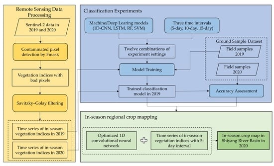
2. Materials and Methods

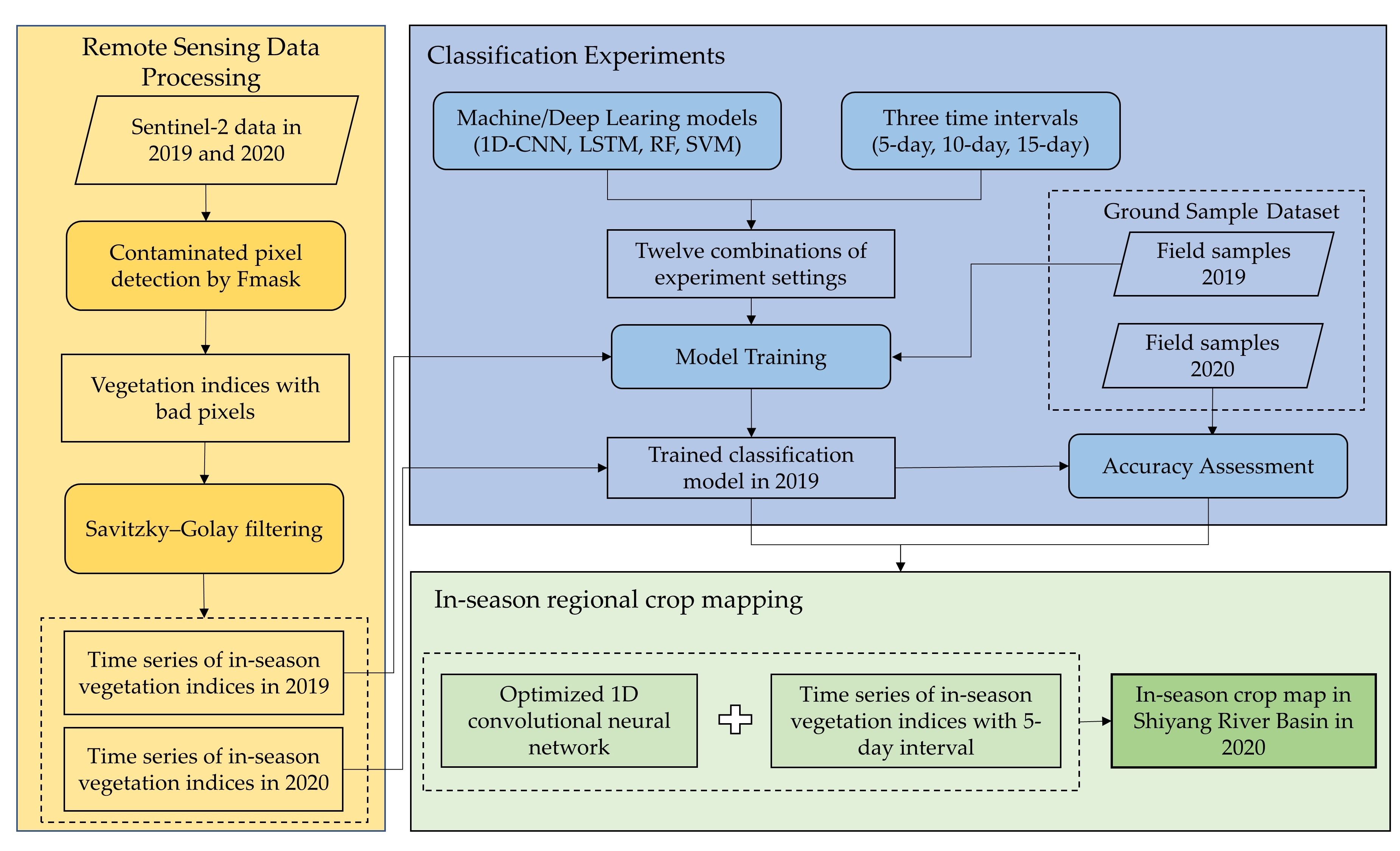
2.1. Overview of the Study Area

The Shiyang River Basin is located in central Gansu Province, north of the Qilian Mountains (37.2–39.5°N, 101.1–103.2°E), in the eastern part of the arid and semi-arid region of northwestern China, and it has a total area of about 40,300 km² (Figure 1). The Shiyang River Basin has a typical continental temperate arid climate. The evapotranspiration in the study area exhibits large spatial and temporal heterogeneity. In the southern mountainous areas, the annual precipitation is 300–600 mm and the annual potential evapotranspiration is 700–1200 mm; while in the downstream areas, the annual precipitation is less than 150 mm and the annual potential evapotranspiration is greater than 2000 mm.

The farmland in the Shiyang River Basin covers about 10% of the total area, and it is mainly located in the middle and lower reaches of the Shiyang River. The local cropland heavily relies on irrigation. The main types of crops in the Shiyang River Basin are wheat, corn, sunflower, alfalfa, fennel, and melons. All six crops, except for alfalfa, are grown in a single season system from April to October due to drought and the cumulative temperatures. Wheat is the earliest sown and earliest harvested crop in the study area, and alfalfa is harvested three times between April and October. Corn, fennel, and sunflower have essentially the same growing period. They are sown in late April and harvested in early September, with a longer growing period than wheat. The melons grown in the study area can be divided into early (sown in late April and harvested in late August) and late (sown in mid-May and harvested in late September) melons according to their different growing seasons.

2.2. Data and Processing

2.2.1. Sentinel-2 Data Products

In this study, the Sentinel-2 L2A product (the bottom atmosphere reflectance product) was used as the primary data source for the crop classification, and the L1C product (the top atmosphere reflectance product) was selected as a secondary data source for cloud detection. Eleven tiles of Sentinel-2 images were acquired to achieve full coverage of the entire Shiyang River Basin. The Sentinel-2 L2A and L1C products for the 2019 and 2020 time series were downloaded from the official European Space Agency (ESA) data distribution website (https://scihub.copernicus.eu (accessed on 1 January 2021)). In total, 1606 images from the L2A product and 1606 images from the L1C product acquired from March to October in 2019–2020 were compiled and used for early-season crop identification.

2.2.2. Ground Reference Data

In May and August of 2019, a handheld global positioning system (GPS) instrument was used to record the center coordinates of the cropland plots of the sample crops, the crop types of the typical crops from the plots were recorded, and the ground sample sets of crops were generated by extracting the corresponding pixels from Sentinel-2 images. We collected data from 268 crop plots. The boundaries of the 268 plots were identified using high-spatial-resolution Google Earth images. A total of 16,880 pixels of Sentinel-2 images within the 268 plots were extracted as the ground sample dataset for 2019. In June 2020, the unmanned aerial vehicle (UAV) observations were combined with Google Earth images to obtain the ground truth samples. The 654 crop plots and 27,843 pixels of Sentinel-2 images were extracted as the crop ground samples for 2020. The crop ground sample sets for 2019 and 2020 were used as the training and testing sets for the classification models, respectively. The number of specific crop samples is shown in

Table 1. Summary of training and verification ground samples for six crop types in the Shiyang River Basin in 2019–2020.

Crop Type	Field-Plot Number		Pixel Number
	2019	2020	2019	2020
Wheat	29	58	2636	4030
Corn	62	166	3702	5358
Melon	78	162	3562	6580
Fennel	30	77	1549	1626
Sunflower	39	159	2522	5352
Alfalfa	30	32	2909	4897
Total	268	654	16,880	27,843

, and the locations of the crop samples are shown in Figure 1.

2.2.3. Image Quality Control

Time-series optical images are susceptible to cloud contamination. To remove the contaminated pixels, we applied the Fmask algorithm to detect clouds, cloud shadows, and snow/ice in each Sentinel-2 image [42]. Figure 2 shows the numbers of the high-quality observations of the individual pixels from March to October in the cropland region of the Shiyang River Basin in 2019 and 2020. The overall numbers of observations were 49 from March to October in both 2019 and 2020, and more than 90% of the pixels had more than 20 observations without cloud interference. Compared with the Landsat data, the high temporal resolution of Sentinel-2 resulted in a significant increase in the observation quality and frequency.

2.2.4. Feature Construction

Yi et al. [43] showed that the four differential vegetation indices, built upon the reflectance from the green band (G), the first red-edge band (RE1), the red band (R), the near-infrared band (NIR), and the first short-wave infrared band (SWIR1) of the Sentinel-2 satellite, are the most effective features for crop classification in the Shiyang River Basin. The four vegetation indices used in this study are expressed in Equations (1)–(4):

$$NDVI=\frac{NIR-R}{NIR+R}$$

(1)

$$NDVI45=\frac{RE1-R}{RE1+R}$$

(2)

$$GNDVI=\frac{NIR-G}{NIR+G}$$

(3)

$$NDWI=\frac{NIR-SWIR1}{NIR+SWIR1}$$

(4)

The normalized difference vegetation index (NDVI) was constructed based on the principle that the reflectance of healthy plants is usually higher in the NIR band than in the visible band and it is the most commonly used vegetation index indicator. Given the saturation of the NDVI in areas with high vegetation cover, the green normalized difference vegetative index (GNDVI) was chosen to compensate for the drawbacks of the NDVI [44]. In addition, the RE1 band of the Sentinel-2 data, which is more sensitive to changes in vegetation chlorophyll, was also chosen to construct the vegetation index [45]. The shortwave infrared band is sensitive to leaf moisture and soil moisture and is often used to estimate the vegetation canopy moisture thickness; therefore, we chose the normalized difference water index (NDWI) to reflect the changes in the moisture content [46].

2.2.5. Data Interpolation and Smoothing

To obtain continuous time-series data with regular time intervals, in this study, we used the Savitzky–Golay filter algorithm to smooth and reconstruct the pixel values with cloud interference [47]. The Savitzky–Golay filter method is based on local polynomial least square fitting in the time domain, which is more suitable for filtering data with a limited data length. Two basic conditions need to be met for reconstruction based on Savitzky–Golay filter. First, the satellite vegetation index is a valid proxy for vegetation growth conditions, and second, clouds and harsh atmospheric conditions usually reduce the vegetation index values. Therefore, sudden drops in the vegetation index that are not consistent with the gradual process of vegetation growth changes are treated as noise and are removed. Based on this, the iteration approaching the upper envelope of the vegetation index series using the Savitzky–Golay filter can be used to reconstruct the continuous time-series vegetation index well. The hyperparameters of the Savitzky–Golay filter mainly include the length of the window involved in the fitting and the power of the polynomial fit. In this study, the window length and the power of the polynomial were set to 5 and 3, respectively. In addition, as the normalized difference water index (NDWI) varies under different dry and wet conditions, it does not satisfy the requirements of the Savitzky–Golay filter. Thus, we simply used the linear interpolation method to fill the gaps in the NDWI time series.

3. Methodology

3.1. Classifier

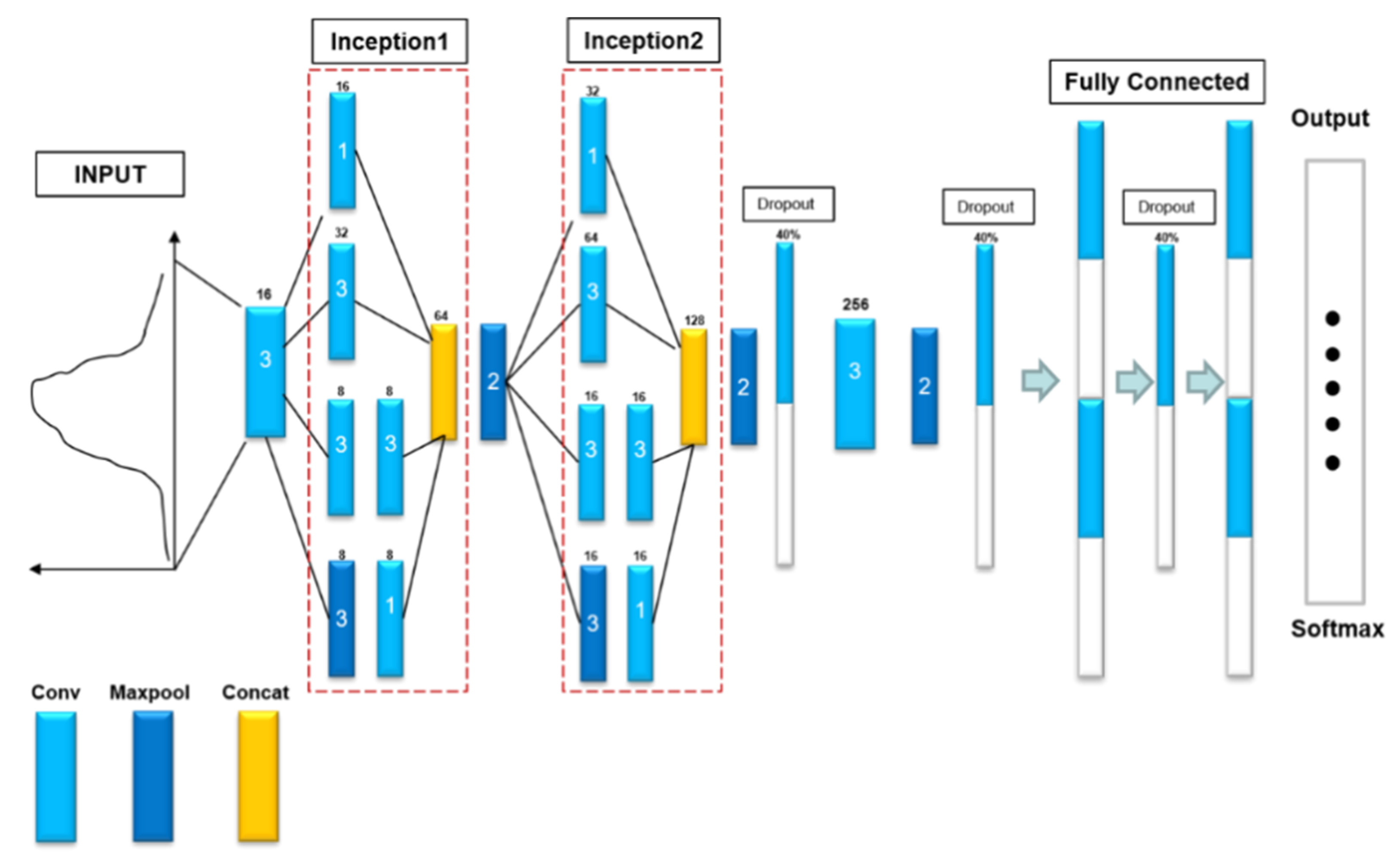
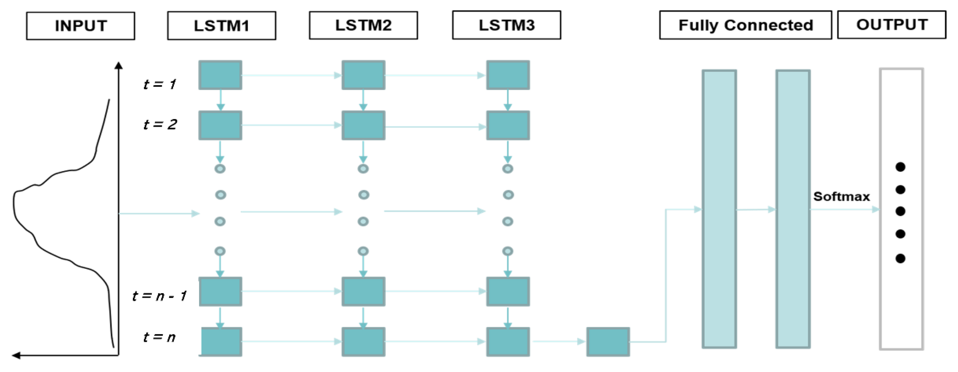
3.1.1. Deep Learning Models

In this study, we selected two deep-learning models to classify the crops based on the four time-series vegetation indexes: the Conv1D network, which is a special type of convolutional network, and the LSTM, which is an RNN. The Conv1D network and LSTM represent two different but effective strategies for representing sequential data. The Conv1D network uses a one-dimensional convolution operator to capture the temporal patterns of the input sequence. The Conv1D network layers can be stacked so that the lower layers focus on the local features and the higher layers summarize the more general patterns to a greater extent. The LSTM units are designed to memorize the values at arbitrary time intervals (long or short). The LSTM improves the efficiency of describing the temporal patterns at different frequencies, which is an ideal feature for analyzing crop growth cycles of different lengths.

Figure 3 shows the architecture of the convolutional network used in this study. The entire convolutional network consisted of two normal convolutional layers with a convolutional kernel size of three and two inception structures used to extract the high-level temporal features. Then, two fully connected layers and a softmax layer are used to output the classification probabilities to obtain the final crop type. The number of channels in the first convolutional module layer was 16, and thereafter, the number of channels in each layer was gradually increased. The final layer of the fully linked layer contained six neurons and was used to output the probabilities of the six crops. The penultimate layer collected information from the previous layer in the form of a planar array, the size of which was determined by the size of the initial input layer. Each of the convolutional modules (light blue squares in Figure 3) contained the convolutional computation, the Batchnorm computation for the batch data normalization, and the rectified linear unit (RELU) activation function for the neuron activation in turn. The inception structure shown in Figure 3 is a classical structure proposed by a Google research team in 2014, which is a parallel structure. The inception structure parallelized the input through a convolutional kernel size of 1, a convolutional kernel size of 3, a convolutional kernel size of 5, and a maximum pooling layer, after which the four parts of the output were concatenated on a channel to obtain the final output. The dropout was a random discarding of a certain percentage of neurons via regularization to prevent overfitting of the model, and we set the activation probability of the neurons to 0.4.

The architecture of the LSTM network used in this study is shown in Figure 4. It contained three layers of LSTM cells for extracting the complex features from the time-series data and two fully connected layers with softmax layers to output the probabilities of the various crops. To prevent overfitting, a dropout layer was added with the same parameter settings used for the dropout in the Conv1D network.

Both the Conv1D and LSTM were constructed based on the Pytorch framework [48]. Both the Conv1D and LSTM used the cross-entropy loss function with L2 regularization as the optimization criterion, and the Adam optimizer was used for the parameter estimation. The learning rate was set to 0.0001, and the batch size was set to 64. The cross-entropy loss function was calculated as follows:

$$loss={\displaystyle \sum }_{i=1}^N{\displaystyle \sum }_{k=1}^K{p}_{i,j}^{true}\log \left(p_{i,j}^{pred}\right)+\lambda {\left|\left|w\right|\right|}^2$$

(5)

In Equation (5), N is the number of training samples, i is the index of the samples, K is the number of target categories (K = 6 in this study), j is the index of the categories, $p_{i,j}^{true}$ and $p_{i,j}^{pred}$ represent the true and predicted probabilities that the ith sample belongs to category j, λ represents the coefficient of the L2 regularization term, and w represents all the parameters in the model that need to be learned.

3.1.2. Shallow Machine Learning Models

In this study, an RF model and an SVM model were used as the baseline models for comparing the classification performances of the different models in different contexts. The scikit-learn package in Python was used to implement the RF and SVM models [49]. The RF algorithm was an integrated classification algorithm based on a bagging strategy with decision tree-based classifiers [50]. The SVM algorithms performed the classification by separating the hyper-planes and performed the non-linear classification using widely used kernel functions [21,51]. RF algorithms and SVM algorithms have been widely used in remote sensing applications and have achieved great success in complex classification tasks [52,53,54]. In this study, a grid-based search strategy was used to select the appropriate model hyper-parameters for constructing the RF and SVM models. The details of the model hyper-parameter selection are presented in

Table 2. Specifications about the hyper-parameters of the two machine-learning models (RF and SVM) used in this study.

Classifiers	Hyper-Parameters	Optional Values	Selected Values
RF	n_estimators	100, 200, 300, 400, 500	500
	max_depth	5, 7, 9, 11, 13, None	13
	min_samples_split	2, 5, 10, 15, 20	2
	min_samples_leaf	1, 2, 5, 10	1
	max_features	log2, sqrt, none	sqrt
SVM	C	0.001, 0.01, 0.1, 1, 10, 100	1
	gamma	0.01, 0.1, 1, 2, 10	2

.

3.2. Experimental Design

Early-season crop identification requires that the model extracts the useful information from remote sensing time-series data with a limited length as early as possible. The process of early crop mapping or early-season crop identification time extraction used in this study is illustrated in Figure 5. Since the crop growing season in the Shiyang River Basin is from April to October, in this study, DOY103 (i.e., the 103rd day of the year) was set as the starting date of the growing season, and the vegetation index data for the subsequent dates were sequentially added to the classifier for the crop classification. The end date of the growing season was set to DOY303. DOY103 was in early April when the crops in the Shiyang River Basin had not yet been sown, and DOY303 was in late October, when the major crops in the basin had already been harvested. In this way, the classification accuracy increased with the length of the time series data over time, and at a particular point in time, the classification accuracy usually reached saturation and stopped increasing. Based on the change in the model’s accuracy as the crop growing season progressed, we chose the time when the accuracy reached stability (classification accuracy greater than 90% of the post-season mapping accuracy level) as the time for the early crop mapping and early identification of each crop in the Shiyang River Basin. To distinguish the effects of the different temporal intervals on the early-season crop identification, three temporal intervals, i.e., 5, 10, and 15 days, were applied. In total, we applied 12 combinations of experimental settings for the three temporal intervals (5, 10, and 15 days) and four classifiers. The ground sample set for 2019 was used for the model training and the ground sample set for 2020 was used to validate the crop classification in 2020. In this study, the confusion matrix and F1 score were used to evaluate the accuracy of the classification results.

It should be noted that for the Conv1D model, the length of the input temporal data affects the number of neurons in the fully connected layer. In the early-season crop identification experiments, the length of the temporal data changed constantly, thus changing the dimensionality of the input data, which increased the workload and complexity of the model tuning. Therefore, when using Conv1D networks for classification, we masked the data with zeros at the time nodes that were not used to fix the input length of the time-series data at 49. This allowed the information contained in the input data to be consistent with that contained in the short time-series data while simultaneously unifying the model’s architecture. For the other three classifiers, masking operations were not applied.

3.3. Accuracy Assessment

In this study, 16,880 crop samples obtained in 2019 were selected as the training sample set and 27,843 crop samples obtained in 2020 were selected as the test sample. For each classification, we measured the performance of the classification by calculating the confusion matrix and the F1 score for the test sample set. The overall accuracy (OA), user accuracy (UA), and producer accuracy (PA) are the three basic evaluation metrics in remote sensing classification. They depict the reliability of the classification results from different perspectives and are the most commonly used evaluation metrics for land cover classification at present. The OA is the probability that the classification labels of all of the classified samples are the same as the actual category labels. The UA is a conditional probability metric that describes the probability that a randomly selected sample from the classification results will have a category label that agrees with the actual category label on the ground. The PA is also a conditional probability metric that describes the probability that any sample taken from the test data will have the same category label as its test category label in the classification results. For each category, the F1 score describes the summed average of the PA and UA for a single category which balances the PA and UA. The F1 score is calculated as follows:

$$F{1}_{class}=2\times \frac{p{a}_{class}\times u{a}_{class}}{p{a}_{class}+u{a}_{class}}$$

(6)

where $\mathrm{F}{1}_{\mathrm{class}}$ is the F1 score for a single class, ${\mathrm{pa}}_{\mathrm{class}}$ is the PA for a single class, and ${\mathrm{ua}}_{\mathrm{class}}$ is the UA for a single class.

In this study, Card’s correction was used to calibrate the PA considering the proportion bias of the ground sample sets and also to compute the 95% confidence interval in the accuracy evaluation of the thematic map [55].

McNemar’s test was used to evaluate the statistical significance of the different scenarios of classification described in Section 5.2 [56].

4. Results

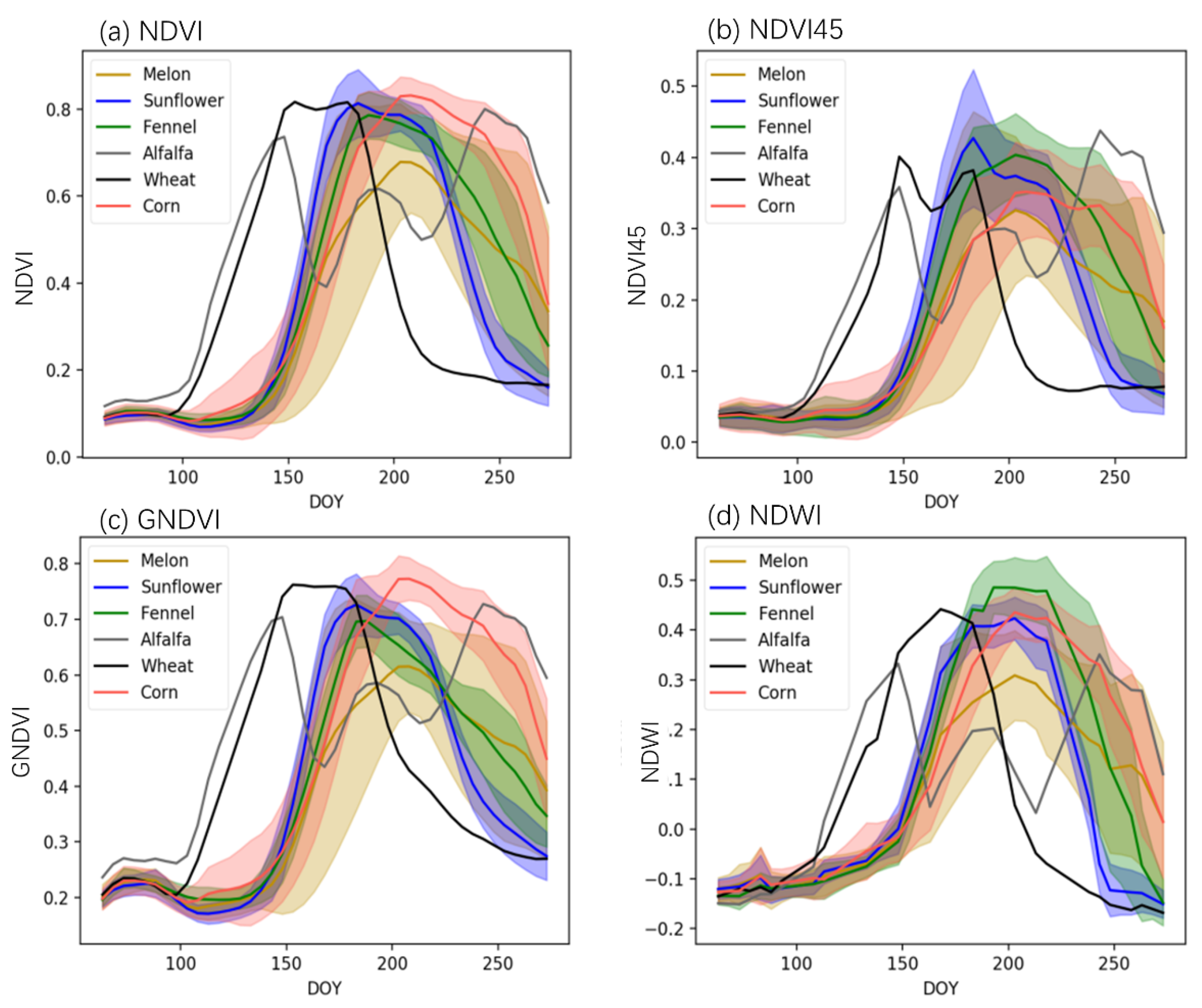
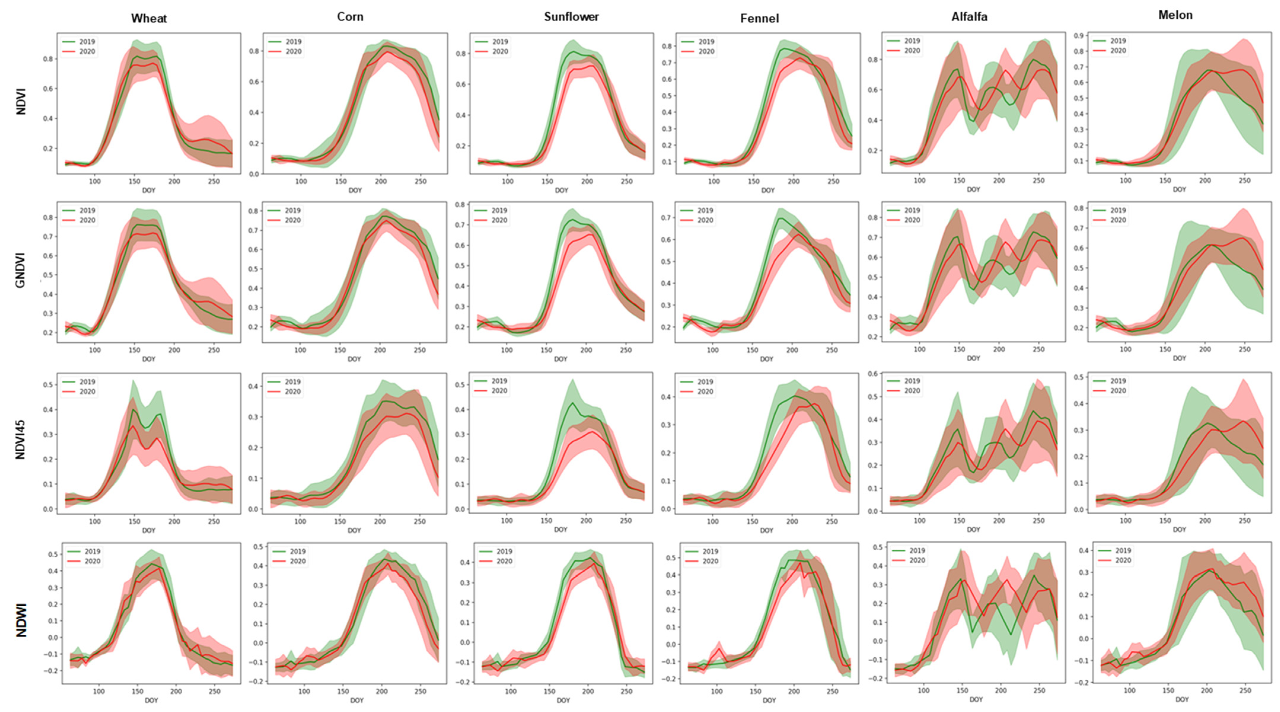
4.1. Crop Growth Characteristics

Figure 6 shows the four time-series vegetation index curves for the six crops in the Shiyang River Basin. The time-series vegetation index curves for wheat and alfalfa were significantly different from those of the other four crops. The vegetation index of wheat started to increase on around DOY100, reached saturation on around DOY150, started to decrease on around DOY175, and reached a relatively small and stable value on DOY200. The vegetation index of the alfalfa exhibited fluctuating characteristics, reaching local maxima on around DOY150, DOY200, and DOY250, and reaching local minima on around DOY165, DOY220, and DOY275 due to multi-harvesting. The other four crops (i.e., sunflower, corn, fennel, and melons) exhibited time-series vegetation index curves with similar characteristics due to their similar growth cycles. There was also a large overlap in the buffer section of these four vegetation indices, making crop classification more difficult. However, differences still existed. First, the peak stage in the sunflower vegetation index was narrower, followed by fennel, while corn had the widest peak. This was mainly due to the differences in the harvest dates of these three crops. In addition, corn had a higher NDVI and GNDVI than the other four crops in the mid to late growing season, but this was not reflected in the NDVI45 and NDWI. The fennel had the highest NDWI in the middle of the crop growing season. These differences suggest that extracting the deeper differences hidden in the time-series vegetation indices was the key to identifying the different crops.

4.2. Classification Performances of the Different Combinations of Classification Strategies

In this study, four classifiers (Conv1D network, LSTM network, RF algorithm, and SVM algorithm) and three different time-series data intervals (5, 10, and 15 days) were tested for classification using the 2019 samples for training and the 2020 samples for testing. We repeated the procedure for each scenario five times and then averaged the overall accuracy to reduce the uncertainty of the stochasticity. The mean value and standard error of the overall accuracy of each scenario are shown in Figure 7. The results show that the maximum overall classification accuracy achieved in this study was 0.87 when using a Conv1D network. Therefore, the time when the overall accuracy first exceeded 0.8 (greater than 90% of the maximum accuracy) was used as the time for the early crop mapping in the Shiyang River Basin.

The different classifiers had different classification performances. The best classification accuracy was 0.87 for the Conv1D when using the full time-series data (i.e., end-of-season mapping), followed by 0.85 for the LSTM network and the SVM network, while the accuracy was only 0.82 for the RF algorithm. The classification accuracies of the four algorithms exhibited a similar pattern over time when mapping within the growing season. The classification accuracy improved rapidly in the early and middle parts of the growing season, plateaued in the middle of the growing season, and increased slowly in the late part of the growing season. However, the rate of increase of the classification accuracy and the time it took to reach stability were not the same for all four classification algorithms. The overall accuracies of the Conv1D network and the LSTM network increased rapidly between DOY160 and DOY200. The classification accuracy of the Conv1D network exceeded 0.8 for the first time on DOY198, with the actual classification accuracy being 0.82 (Figure 7a). The classification accuracy of the LSTM network reached 0.8 for the first time on DOY208 (Figure 7a). The overall accuracies of the RF and SVM algorithms increased between DOY140 and DOY240 and reached 0.8 for the first time on DOY258 and DOY238, respectively (Figure 7c,d), with significantly lower rates of increase of the classification accuracy than those of the two deep-learning algorithms. Considering that the data for the previous and next two phases need to be used when filtering and smoothing the time-series vegetation index data, the actual early mapping times for the Conv1D, LSTM, RF, and SVM algorithms were DOY208 (late July), DOY218 (early August), DOY268 (late September), and DOY248 (early September), respectively. The earliest mapping times for the SVM algorithm and the RF algorithm were later than DOY238 (end of August), which was already in the harvesting period for the summer crops in the Shiyang River Basin. Thus, it was concluded that the RF and SVM were not effective in early crop identification.

Figure 7 also shows that the time-series data for the different temporal intervals had different classification performances. When using the Conv1D network for the classification, the overall accuracy of the crop classification using the 5-, 10-, and 15-day interval data exceeded 0.8 for the first time on DOY198, DOY203, and DOY218, respectively; while for the LSTM network, the classification accuracy when using the 5-, 10-, and 15-day interval data exceeded 0.8 on DOY208, DOY228, and DOY253, respectively. The SVM algorithm and RF algorithm performed the worst in this study, with classification accuracies exceeding 0.8 for all three intervals later than DOY238 and DOY258, respectively, and thus, they could not be used for the early crop identification. In addition, the two shallow machine-learning algorithms (the RF and SVM) had significantly lower classification accuracies for post-seasonal mapping when using 10- and 15-day interval data than when using 5-day interval data, whereas this did not occur when using the Conv1D and the LSTM networks. This may be due to the information redundancy of the multi-temporal features in the 5-day interval data, which reduced the classification accuracy of shallow machine-learning algorithms that use these features directly as the basis for the classification. In contrast, both the Conv1D and the LSTM networks automatically extracted the hidden features from the temporal data using their respective non-linear arithmetic units, reducing the effect of the information redundancy.

In conclusion, the early crop identification times in the Shiyang River Basin obtained using different classifiers with different intervals of time-series data varied. The Conv1D and the LSTM networks completed the classification task earlier and with higher accuracies than the SVM algorithm and the RF algorithm. In addition, a 5-day interval of data allowed the earliest actual early-season crop identification times to be obtained. In this study, the combination of the Conv1D network and a 5-day interval of time-series data was used to obtain the earliest (DOY198) crop identification with a high accuracy (OA = 0.82).

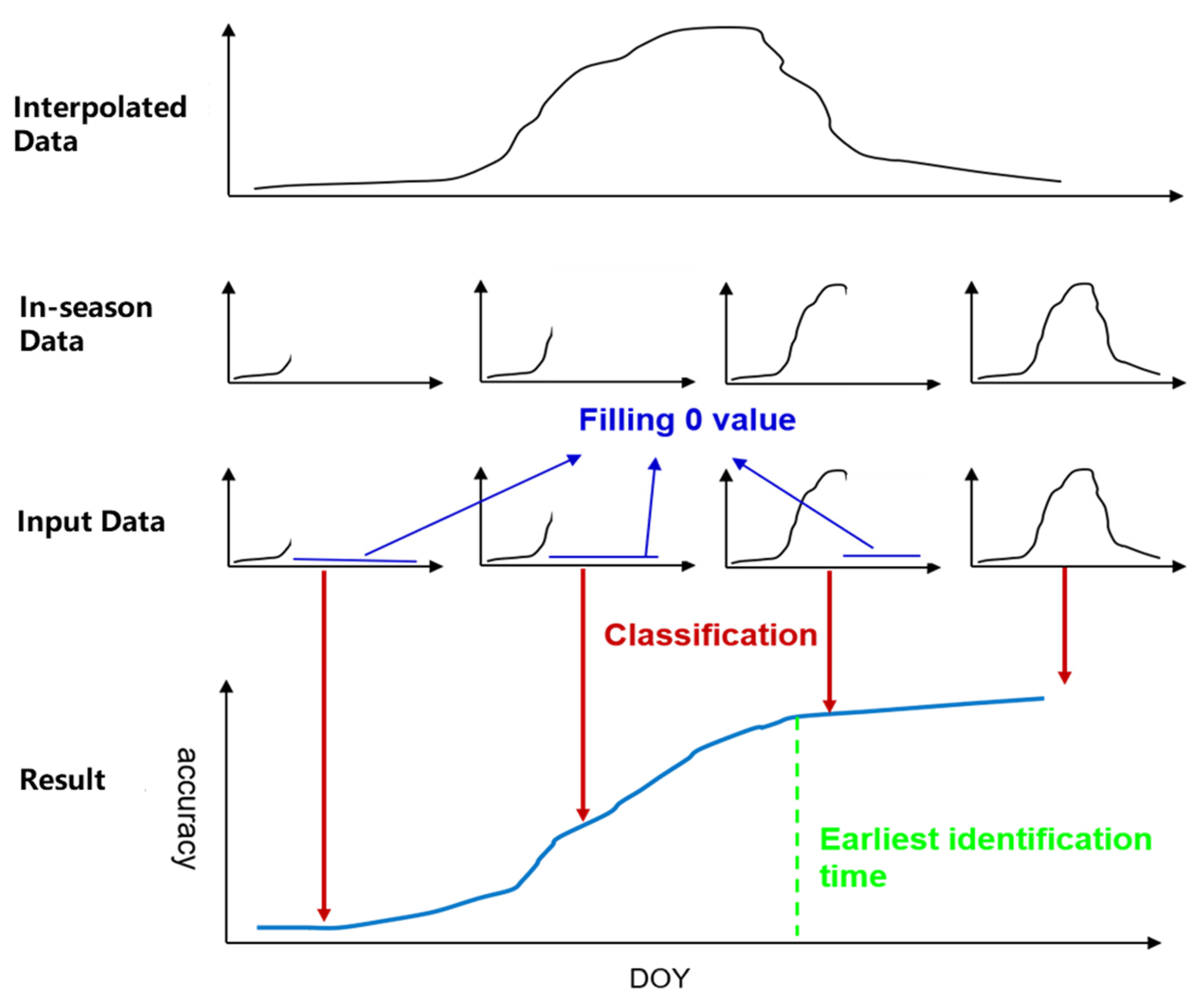
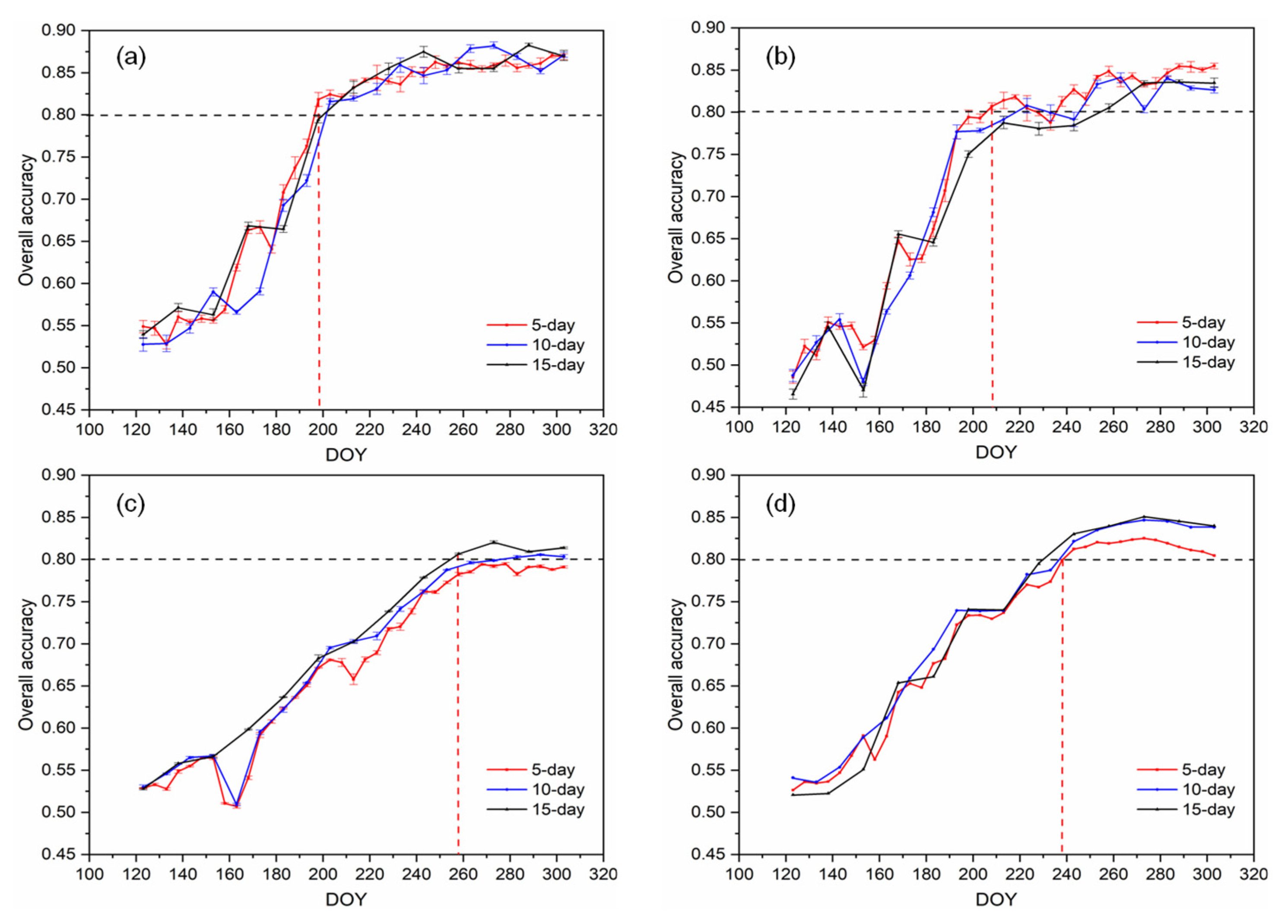
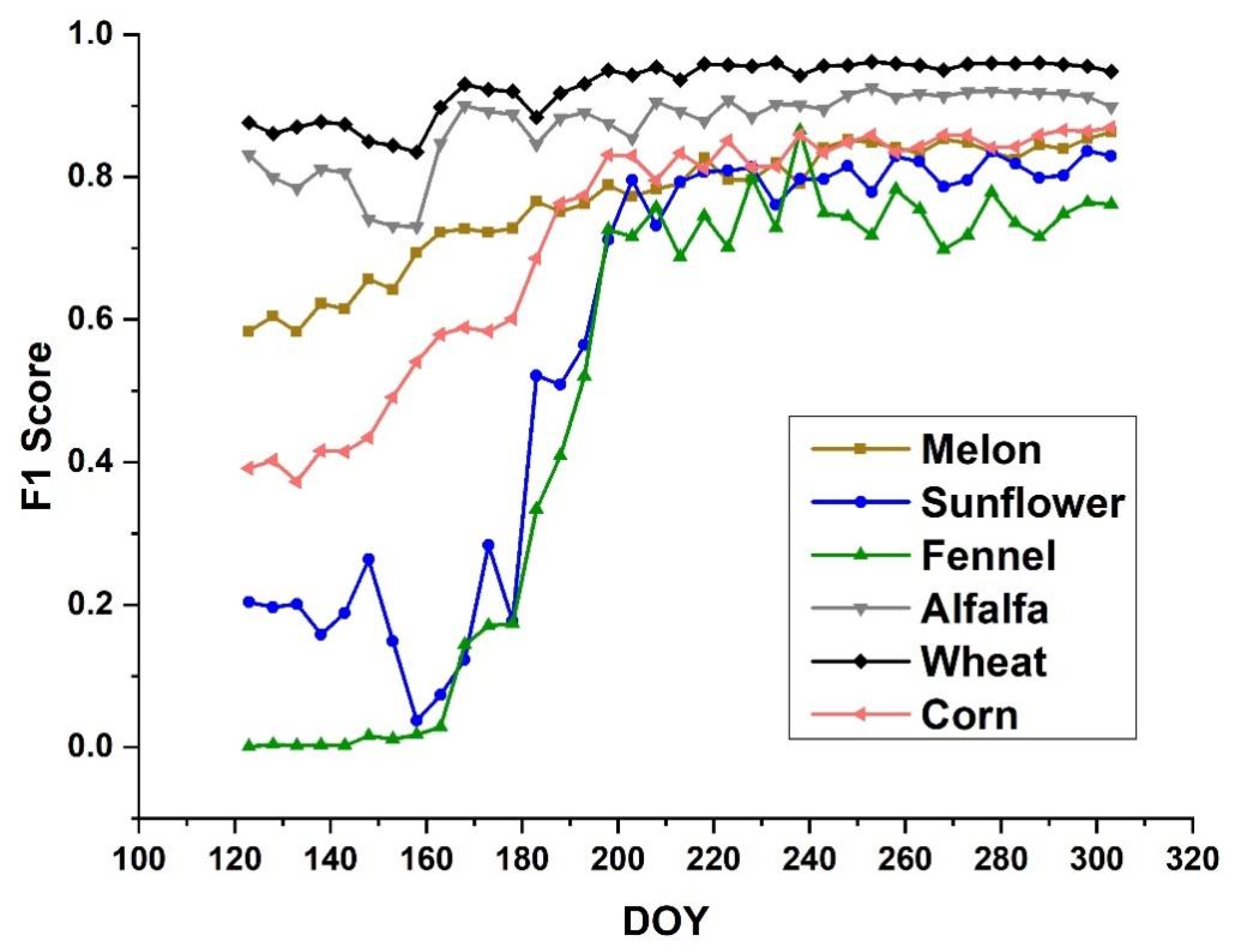
4.3. Early Identification Time for Each Crop

By comparing the experimental results for the 12 classification scenarios, we found that the Conv1D network and 5-day interval of Sentinel-2 time-series vegetation index data could identify the crops more efficiently within the season. The results shown in Figure 7 indicate that the earliest time when the crops could actually be effectively identified in the Shiyang River Basin was on around DOY210, which was in the middle of the crop growing season in the Shiyang River Basin. Furthermore, we analyzed the earliest identifiable time for each crop, and the F1 score for each crop was found to vary (Figure 8). The F1 score for wheat was almost stable on around DOY168, with an F1 score of 0.95. The alfalfa also achieved a stable F1 score on around DOY168, with an F1 score of 0.9. The earliest identifiable time for corn was on around DOY198, with an F1 score of 0.82. The fennel and sunflower had similar F1 scores, with low F1 scores before DOY180 and increasing rapidly after DOY180. The F1 score for melons did not exhibit a clear turning point, reaching 95% of the F1 score on around DOY200. Because the vegetation index at every time point was calculated using two data points before and two data points after the current phase in the interpolation of the temporal data, the actual earliest identifiable times for the wheat and alfalfa were on around DOY180, and those for the remaining four crops were on around DOY210. Figure 9 shows the corresponding phenological stages at the earliest identification times for five of these crops. The earliest identifiable time for wheat in the Shiyang River Basin was in its flowering stage, that of alfalfa was in the first harvest stage, that of corn was in the early heading stage, and those of fennel and sunflower were both in the transition period between the flowering and grouting stages. The earliest identification time for the melons was early August, but the varieties of the melons and the complexity of their phenological stages made it impossible to determine which phenological stage corresponded to their early identification time.

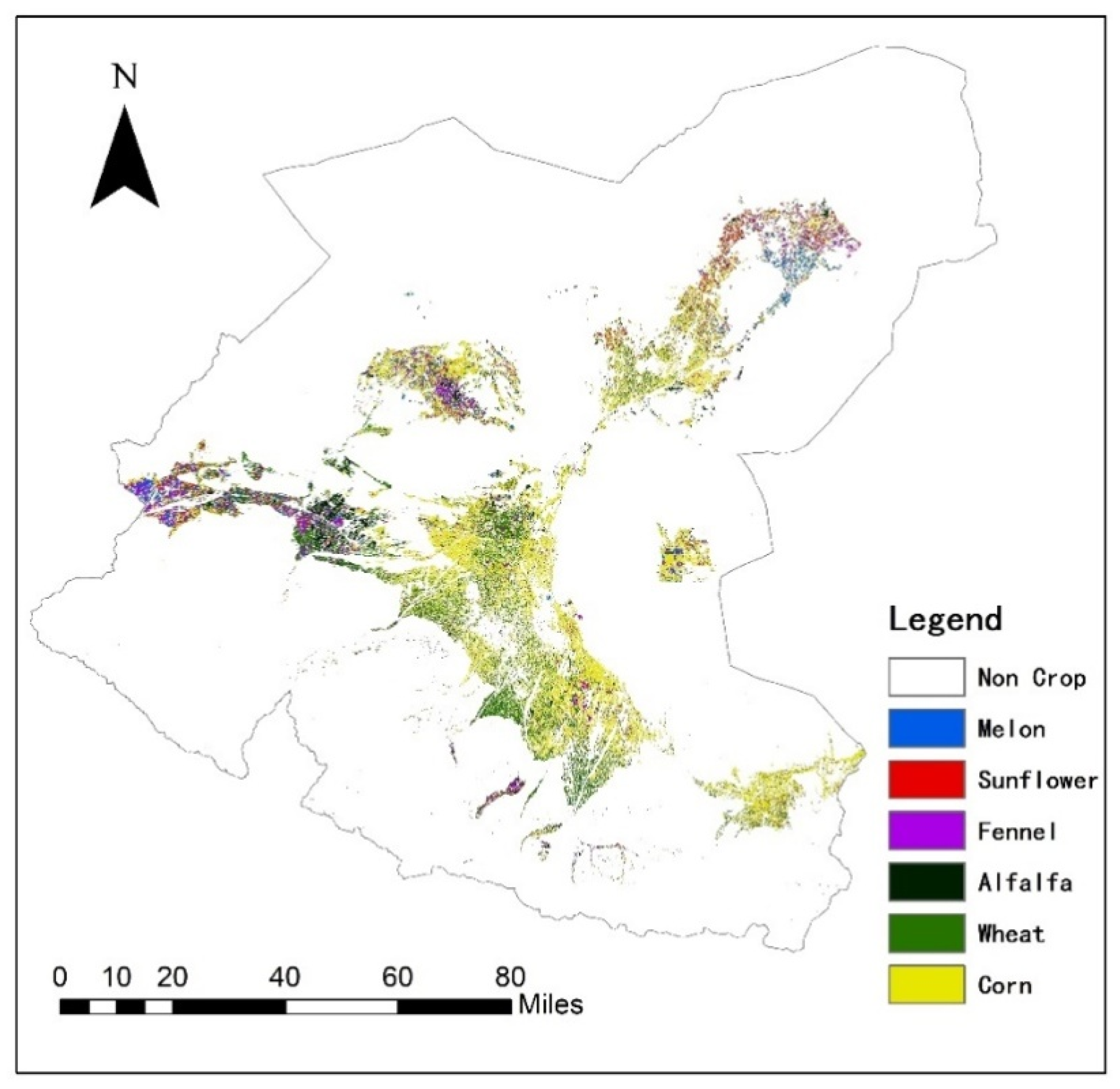
4.4. Early Crop Mapping in the Shiyang River Basin

We used short time-series data from DOY63 to DOY198 (actual cut-off date DOY208) and the Conv1D network algorithm to conduct early crop mapping in the Shiyang River Basin (Figure 10). These maps were created using only early-season images from 2020, and the Conv1D classifier was trained using 2019 data without relying on the field samples collected in 2020. As can be seen from the maps, the Shiyang River Basin was dominated by food crops, with corn being the most widely grown and distributed throughout the basin, followed by wheat, which was mainly grown in the middle reaches of the Shiyang River Basin and close to the urban areas of Wuwei City. The cash crops such as sunflower, melons, and fennel were mainly located in the lower reaches of the Shiyang River Basin, in the northern part of Minqin County, which was extremely arid and economically backward. The fragmentation and small sizes of the local crop plots inevitably led to misclassification of small patches and pixels on the plot boundaries. The confusion matrix after proportion calibration for this early mapping is presented in

Table 3. Confusion matrix of the early-season crop map for 2020 in the Shiyang River Basin obtained using the Conv1D network. The proportion calibration and 95% confidence interval calculation were based on the method of Olofsson et al. [55] for the PA, UA, and OA using the map accuracy library in the R language. The proportion was calculated by using the pixel number of each crop in the predicted map. To calculate the 95% confidence intervals, the sample size was set to 654, which is the total number of independent samples from the different crop plots, to avoid excessively narrow confidence intervals.

Actual Types	Predicted Types						Total	PA
	Melons	Sunflower	Fennel	Alfalfa	Wheat	Corn
Melons	4843	328	353	150	159	747	6580	0.58 ± 0.09
Sunflower	484	3998	197	265	5	403	5352	0.51 ± 0.10
Fennel	159	70	1280	32	3	82	1626	0.76 ± 0.16
Alfalfa	223	150	60	4047	108	309	4897	0.78 ± 0.09
Wheat	50	6	5	68	3876	25	4030	0.98 ± 0.03
Corn	198	143	52	17	41	4907	5358	0.97 ± 0.02
Total	5957	4695	1947	4579	4192	6473	27,843
Proportion	0.1267	0.0590	0.0428	0.1266	0.2108	0.4341	1
UA	0.81 ± 0.06	0.85 ± 0.06	0.66 ± 0.11	0.88 ± 0.11	0.93 ± 0.07	0.76 ± 0.07
	OA	0.81 ± 0.04			Kappa	0.79

. The overall accuracy of the crop classification in the Shiyang River Basin using the short time-series data for DOY103 and DOY198 was 0.81, with a kappa coefficient of 0.79. The wheat had the highest PA and UA and was identified the most accurately, while the fennel had a low UA of 0.64, and the melons were susceptible to misclassification as fennel. The melons and corn were also misclassified, which was mainly due to the similarity of the agricultural calendars of these crops. Since the proportions of the melon and sunflower in the sample set were not consistent with the crop distribution in the basin, the proportion-corrected PA values for the melon and sunflower were low (0.58 and 0.51).

5. Discussion

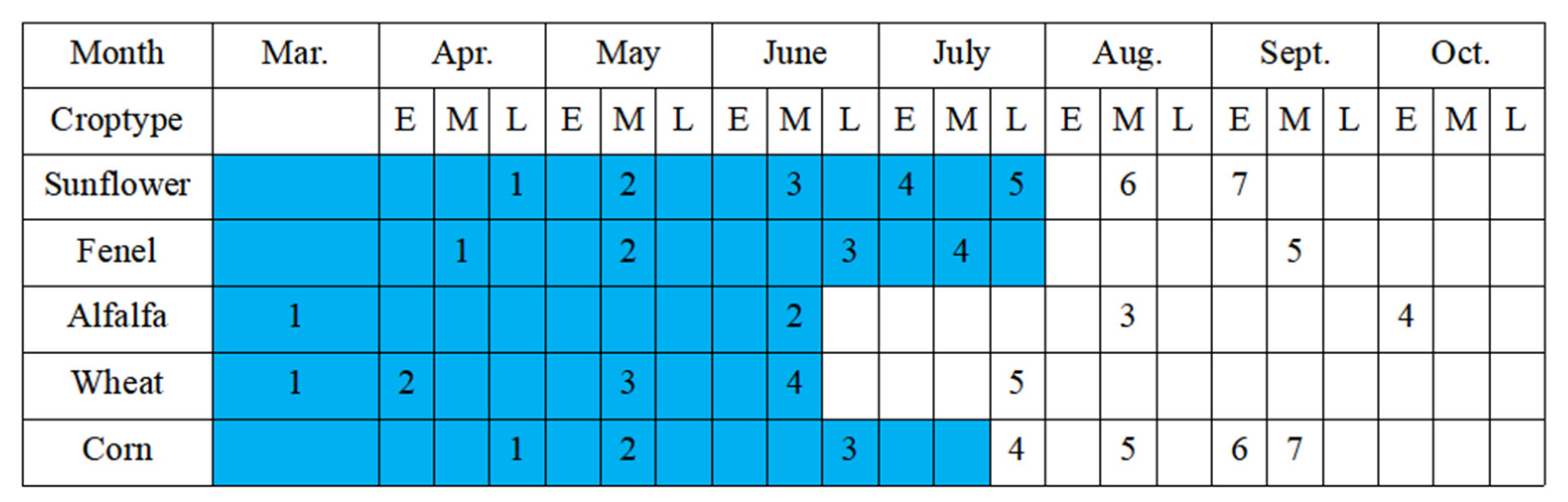
5.1. Influence of Crop Spectral and Phenological Characteristics on Early Identification Times

We obtained early crop mapping times and early identification times for each of the six crops in the Shiyang River Basin based on 5-day interval time-series Sentinel-2 vegetation index data and a Conv1D network classifier with interannual migration (Figure 7, Figure 8 and Figure 9). The early mapping times for the crops in the Shiyang River Basin were DOY200–DOY210 (end of July), which was in the middle of the growing season of the crops in the Shiyang River Basin. This is similar to previous findings in that the use of more images improves the accuracy of crop mapping and that a higher accuracy can be obtained in the middle of the growing season [30,57]. In addition, we further analyzed the phenological stage in which the early identification times of the six crops were located and their spectral performances.

The earliest identification time for wheat was during its flowering period (DOY 170) when the wheat had completed its nutritional reproductive phase and the vegetation cover was at its peak. In this stage, wheat had a significantly higher vegetation index, effectively increasing the identifiability of wheat compared with the other crops. The earliest identification time for alfalfa was during its first harvest stage (DOY170), and the variations in the four vegetation indices from low to high to low (Figure 6) also effectively reflected the fact that the first harvest of alfalfa was the key period for differentiating the alfalfa from the other crops. The early identification times for corn, sunflower, and fennel were during the early tassel, early grouting, and flowering stages, respectively. It should be noted that the F1 scores for corn, sunflower, and fennel increased rapidly after the beginning of July (DOY180) and reached a steady state on around DOY200 (Figure 8). This was because all three crops were in the nutrient stage of growth with rapid rootstock and vegetation cover development before July (DOY180), but the simple increase in greenness did not result in large differences between the four vegetation indices (Figure 6). However, the plants entered the reproductive growing stage after July and differentiated into distinctive reproductive organs, providing the classifiers with more information to improve the performance. For example, the fennel exhibited an umbel shape and was bright yellow in color. The sunflower exhibited a head-shaped inflorescence and was orange in color. The corn exhibited a panicle or fleshy spike and was light yellow in color. The different shapes, pigment levels, and moisture contents of the crops cause the spectral properties of the crops to differ. This was also reflected by the performances of the four vegetation indices. The NDVI and GNDVI of corn were higher than those of fennel and sunflower after July, and the NDWI of fennel was relatively high (Figure 6). These differences were crucial in distinguishing between corn, sunflower, and fennel. In addition, previous studies were able to validate the reliability of our results, i.e., the use of high-temporal-resolution Sentinel-2 type data allowed for the effective identification of summer crops (e.g., similar to corn) in the heading/flowering stage of the crops [57]. The earliest identification time for the melons was around DOY200, although it was not possible to determine the phenological stage of the melons corresponding to this period. However, as can be seen in Figure 6, the four vegetation indices of melons peaked on around DOY200, indicating that the melons had completed their nutritional growth phase and have entered their reproductive growth phase. In addition, the four vegetation indices for the melons on around DOY200 were lower than those for the sunflower, fennel, and corn, all of which had similar growing seasons. These differences suggest that late July to early August is a critical time for identifying melons.

5.2. Factors Decreasing the Accuracy of the Early Crop Mapping

Compared with the crop classification using samples and full-season data acquired in the mapping year, we made some trade-offs between the timeliness and accuracy for early-season crop identification. First, we applied our model trained using the 2019 samples to map the crops in 2020, and then, we used short time-series data (28 images) before DOY198 to advance the timing of the within-year mapping. These two strategies inevitably had an impact on the accuracy of the remote sensing classification of the crops. To understand the impacts of these two strategies on the classification accuracy of the early crop mapping, we constructed three classification scenarios, including crop classification using historical samples and early-season images (HSES), using historical samples and full-season images (HSFS), and using samples and full-season images for the mapping year (SFSMY). The HSFS scenario refers to transferring the classifier trained using the crop samples and full time-series data (49 images) for 2019 to the 2020 time-series data. The SFSMY scenario refers to training the classifier using the crop samples and full time-series data (49 images) for 2020 to predict the 2020 time-series data. Compared with the HSES scenario, which uses historical samples and short time-series data, the HSFS scenario uses historical samples and full time-series data and the SFSMY scenario uses samples from the mapping year and the full time-series. Hence, the differences in the accuracies of the three scenarios can help us understand the impact of the two strategies on the classification. We quantitatively compared the results of the three scenarios (

Table 4. Accuracy of crop classification in the Shiyang River Basin using different mapping methods.

	HSES			HSFS			SFSMY
	PA	UA	F1 Score	PA	UA	F1 Score	PA	UA	F1 Score
Melons	0.74	0.81	0.77	0.85	0.87	0.86	0.95	0.95	0.95
Sunflower	0.75	0.85	0.80	0.78	0.89	0.83	0.96	0.96	0.95
Fennel	0.78	0.64	0.70	0.95	0.66	0.78	0.94	0.94	0.94
Alfalfa	0.83	0.88	0.85	0.84	0.96	0.90	0.98	0.98	0.98
Wheat	0.96	0.93	0.94	0.95	0.95	0.95	0.97	0.99	0.97
Corn	0.92	0.76	0.83	0.93	0.82	0.87	0.96	0.96	0.96
OA	0.83			0.87			0.96
Kappa	0.79			0.84			0.95

) and conducted a mutual confidence test (

Table 5. Results of McNemar’s test on the crop classification scenarios using different mapping methods. The McNemar’s test for a single crop was conducted in a binary classification system. All of the tests shown were two-sided, and a 10% level significance was selected.

	HSES vs. HSFS		HSFS vs. SFSMY
	Z Value	Significant?	Z Value	Significant?
Melons	4.98	YES, 5%	1.76	YES, 10%
Sunflower	4.09	YES, 5%	1.99	YES, 5%
Fennel	2.92	YES, 5%	1.86	YES, 10%
Alfalfa	0.34	NO	1.33	NO
Wheat	0.13	NO	0.50	NO
Corn	1.98	YES, 5%	1.79	YES, 10%
Total	5.49	YES, 5%	2.54	YES, 5%

) using McNemar’s test (Foody, 2004). It should be noted that only the original 654 samples from the different plots were used to conduct McNemar’s test in order to reduce the uncertainty caused by dependent samples. As is shown in Table 4 and Table 5, the HSFS and SFSMY scenarios significantly outperformed the HSES scenario, and the OA values were 0.04 and 0.13 higher, with a 5% significance level. This indicates that the spectral variations and the lack of information from the middle and late stages of the growing season both decreased the accuracy of the early crop mapping. It should be noted that the significantly higher accuracy indicates that the spectral variations in the crop itself between 2019 and 2020 in the Shiyang River Basin were the more important factor limiting the accuracy of the early crop mapping.

In addition, we analyzed the classification accuracy performances for the crops obtained using the three different mapping strategies (i.e., HSES, HSFS, and SFSMY). The F1 score of the HSES for the melons decreased significantly by 0.09 compared with that of the HSFS, and by 0.18 compared with that of the SFSMY. The F1 scores of the HSES for the fennel decreased significantly by 0.08 and 0.16, respectively, compared with the HSFS and the SFSMY, respectively. This suggests that the interannual spectral variation and information deficits caused by the use of short time-series data had a serious impact on the accuracy of the melon and fennel identifications, and these impacts were at a similar level. This can be explained in Figure 6 and Figure 11. The vegetation index values for the fennel and melons after DOY198 exhibited larger differences compared with those of the other crops (Figure 6), and the vegetation index values of the fennel and melons also exhibited obvious changes between 2019 and 2020 (Figure 11). Compared with the HSFS and SFSMY, the F1 scores of the HSES decreased by 0.03 and 0.12 for sunflower, and by 0.04 and 0.13 for corn. This suggests that the spectral variations in the sunflower and corn between the two years were a major factor reducing their early mapping accuracies. Compared with the HSFS and SFSMY, the F1 scores slightly decreased for wheat by 0.1 and 0.3; however, these differences were not statistically significant. This indicates that spectral features before DOY198 were sufficient to identify wheat, and the interannual spectral variations influenced the wheat identification to a limited level. The F1 score of the HSES for alfalfa decreased by 0.05 and 0.13 compared with the HSFS and SGSMY, but the differences were not statistically significant, and the influence of the interannual spectral variations and short time-series data were not significant based on the results of the McNemar test. In conclusion, the early crop mapping accuracies of the six crops in the Shiyang River Basin decreased by different degrees compared with the mapping of the crops using samples and full-season data acquired in the mapping year, and the reasons for the decrease in the accuracies of the mapping of the six crops were also different. Moreover, identifying fennel and melon in the early growing season was challenging due to the large interannual spectral variations and smaller spectral differences in the early growing season.

5.3. Limitations and Future Work

The field samples in this study were not randomly distributed in the Shiyang River Basin due to the difficulty of conducting fieldwork in this area. The central and southern parts of the Shiyang River Basin are dominated by corn and spring wheat. The northern part of the Shiyang River Basin had a more complex planting structure and was dominated by corn, melon, fennel, sunflower, and alfalfa. In recent years, the wheat planting area has decreased significantly in the northern part of the basin because of the lower water use efficiency. The spring wheat samples were mainly collected in the central and southern parts of the Shiyang River Basin. Among the crops in the Shiyang River Basin, spring wheat has a unique growing season that starts much earlier (March to earlier April) and is therefore easier to identify. For corn, no significant difference in variety and growing season existed in the Shiyang River Basin. Non-randomly distributed wheat and corn samples can also capture their spectral attributes (Figure 6). For field sampling in the northern part of the basin, we visited the main production zones of each crop and collected samples from each zone. The sampling strategy based on local knowledge partially compensates the uncertainties caused by the non-random sample distribution. Future studies can be improved by using random samples.

The minimum mapping unit used for the crop classification and crop type thematic map developed in this study are pixels. Future research should consider testing our methodology using objects (fields) as minimum mapping units as this will reduce within-field variations, which may improve classification accuracies.

6. Conclusions

In this study, we investigated the potential of using deep-learning algorithms and time-series Sentinel-2 data for early crop identification in the Shiyang River Basin. We conducted early-season crop identification experiments on four classifiers (Conv1D, LSTM, RF, and SVM) and time-series Sentinel-2 data with three different interval lengths (5, 10, and 15 days) for six crops in the Shiyang River Basin. By comparing the results of the different scenarios, we found that the two deep-learning algorithms performed better than the two shallow machine-learning algorithms in identifying the early-season crop types. The use of time-series Sentinel-2 data with a 5-day interval as the input of the Conv1D network yielded a higher accuracy in terms of earlier early crop mapping in the Shiyang River Basin. Both the influences of crop physical properties and the mapping strategy have been discussed in detail. We found that the interannual variations in the crops’ spectral properties were the main factor that reduced the accuracy of the early crop mapping in the Shiyang River Basin compared with the mapping of the crops using samples and full-season data acquired in the mapping year. By employing frequently available remote sensing data and deep-learning methods, in this study, we systematically analyzed the possibility of conducting early-season crop identification in highly heterogeneous regions, which may have applications such as more effective crop yield prediction, improved agricultural disaster prevention, and better planting structure optimization.

References

1. Ozdogan, M. The spatial distribution of crop types from modis data: Temporal unmixing using independent component analysis. Remote Sens. Environ. 2010, 114, 1190–1204. [Google Scholar] [CrossRef]
2. See, L.; Fritz, S.; You, L.; Ramankutty, N.; Herrero, M.; Justice, C.; Becker-Reshef, I.; Thornton, P.; Erb, K.; Gong, P.; et al. Improved global cropland data as an essential ingredient for food security. Glob. Food Secur. 2015, 4, 37–45. [Google Scholar] [CrossRef]
3. Franch, B.; Vermote, E.F.; Becker-Reshef, I.; Claverie, M.; Huang, J.; Zhang, J.; Justice, C.; Sobrino, J.A. Improving the timeliness of winter wheat production forecast in the united states of America, Ukraine and china using modis data and ncar growing degree day information. Remote Sens. Environ. 2015, 161, 131–148. [Google Scholar] [CrossRef]
4. Wardlow, B.D.; Callahan, K. A multi-scale accuracy assessment of the modis irrigated agriculture data-set (mirad) for the state of nebraska, USA. GIScience Remote Sens. 2014, 51, 575–592. [Google Scholar] [CrossRef]
5. Jia, K.; Wu, B.; Li, Q. Crop classification using hj satellite multispectral data in the north china plain. J. Appl. Remote Sens. 2013, 7, 073576. [Google Scholar] [CrossRef]
6. Immitzer, M.; Vuolo, F.; Atzberger, C. First experience with sentinel-2 data for crop and tree species classifications in central europe. Remote Sens. 2016, 8, 166. [Google Scholar] [CrossRef]
7. You, N.; Dong, J. Examining earliest identifiable timing of crops using all available sentinel 1/2 imagery and google earth engine. ISPRS J. Photogramm. Remote Sens. 2020, 161, 109–123. [Google Scholar]
8. Hao, P.; Zhan, Y.; Wang, L.; Niu, Z.; Shakir, M. Feature selection of time series modis data for early crop classification using random forest: A case study in kansas, USA. Remote Sens. 2015, 7, 5347–5369. [Google Scholar] [CrossRef] [Green Version]
9. Boryan, C.; Yang, Z.; Di, L. Deriving 2011 cultivated land cover data sets using usda national agricultural statistics service historic cropland data layers. In Proceedings of the 2012 IEEE International Geoscience and Remote Sensing Symposium, Munich, Germany, 22–27 July 2012; pp. 6297–6300. [Google Scholar]
10. Boryan, C.; Yang, Z.; Mueller, R.; Craig, M. Monitoring us agriculture: The us department of agriculture, national agricultural statistics service, cropland data layer program. Geocato Int. 2011, 26, 341–358. [Google Scholar] [CrossRef]
11. Fisette, T.; Davidson, A.; Daneshfar, B.; Rollin, P.; Aly, Z.; Campbell, L. Annual space-based crop inventory for Canada: 2009–2014. In Proceedings of the 2014 IEEE Geoscience and Remote Sensing Symposium, Quebec City, QC, Canada, 13–18 July 2014; pp. 5095–5098. [Google Scholar]
12. Huang, X.; Huang, J.; Li, X.; Shen, Q.; Chen, Z. Early mapping of winter wheat in henan province of china using time series of sentinel-2 data. GIScience Remote Sens. 2022, 59, 1534–1549. [Google Scholar] [CrossRef]
13. Hao, P.; Tang, H.; Chen, Z.; Meng, Q.; Kang, Y. Early-season crop type mapping using 30-m reference time series. J. Integr. Agric. 2020, 19, 1897–1911. [Google Scholar] [CrossRef]
14. Al-Shammari, D.; Fuentes, I.; Whelan, B.M.; Filippi, P.; Bishop, T.F.A. Mapping of cotton fields within-season using phenology-based metrics derived from a time series of landsat imagery. Remote Sens. 2020, 12, 3038. [Google Scholar] [CrossRef]
15. Johnson, D.M.; Mueller, R. Pre- and within-season crop type classification trained with archival land cover information. Remote Sens. Environ. 2021, 264, 112576. [Google Scholar] [CrossRef]
16. Lin, Z.; Zhong, R.; Xiong, X.; Guo, C.; Xu, J.; Zhu, Y.; Xu, J.; Ying, Y.; Ting, K.C.; Huang, J.; et al. Large-scale rice mapping using multi-task spatiotemporal deep learning and sentinel-1 sar time series. Remote Sens. 2022, 14, 669. [Google Scholar] [CrossRef]
17. Cai, Y.; Guan, K.; Peng, J.; Wang, S.; Seifert, C.; Wardlow, B.; Li, Z. A high-performance and in-season classification system of field-level crop types using time-series landsat data and a machine learning approach. Remote Sens. Environ. 2018, 210, 35–47. [Google Scholar] [CrossRef]
18. Konduri, V.S.; Kumar, J.; Hargrove, W.W.; Hoffman, F.M.; Ganguly, A.R. Mapping crops within the growing season across the united states. Remote Sens. Environ. 2020, 251, 112048. [Google Scholar] [CrossRef]
19. Yang, Y.; Ren, W.; Tao, B.; Ji, L.; Liang, L.; Ruane, A.C.; Fisher, J.B.; Liu, J.; Sama, M.; Li, Z.; et al. Characterizing spatiotemporal patterns of crop phenology across north america during 2000–2016 using satellite imagery and agricultural survey data. ISPRS J. Photogramm. Remote Sens. 2020, 170, 156–173. [Google Scholar] [CrossRef]
20. Feng, S.; Zhao, J.; Liu, T.; Zhang, H.; Zhang, Z.; Guo, X. Crop type identification and mapping using machine learning algorithms and sentinel-2 time series data. IEEE J. Sel. Top. Appl. Earth Obs. Remote Sens. 2019, 12, 3295–3306. [Google Scholar] [CrossRef]
21. Löw, F.; Michel, U.; Dech, S.; Conrad, C. Impact of feature selection on the accuracy and spatial uncertainty of per-field crop classification using support vector machines. ISPRS J. Photogramm. Remote Sens. 2013, 85, 102–119. [Google Scholar] [CrossRef]
22. Massey, R.; Sankey, T.T.; Congalton, R.G.; Yadav, K.; Thenkabail, P.S.; Ozdogan, M.; Sánchez Meador, A.J. Modis phenology-derived, multi-year distribution of conterminous U.S. Crop types. Remote Sens. Environ. 2017, 198, 490–503. [Google Scholar] [CrossRef]
23. Zhong, L.; Gong, P.; Biging, G.S. Phenology-based crop classification algorithm and its implications on agricultural water use assessments in california’s central valley. Photogramm. Eng. Rem. Sens. 2012, 78, 799–813. [Google Scholar] [CrossRef]
24. Zhong, L.; Gong, P.; Biging, G.S. Efficient corn and soybean mapping with temporal extendability: A multi-year experiment using landsat imagery. Remote Sens. Environ. 2014, 140, 1–13. [Google Scholar] [CrossRef]
25. Xu, J.; Zhu, Y.; Zhong, R.; Lin, Z.; Xu, J.; Jiang, H.; Huang, J.; Li, H.; Lin, T. Deepcropmapping: A multi-temporal deep learning approach with improved spatial generalizability for dynamic corn and soybean mapping. Remote Sens. Environ. 2020, 247, 111946. [Google Scholar] [CrossRef]
26. Song, X.P.; Potapov, P.V.; Krylov, A.; King, L.; Di Bella, C.M.; Hudson, A.; Khan, A.; Adusei, B.; Stehman, S.V.; Hansen, M.C. National-scale soybean mapping and area estimation in the united states using medium resolution satellite imagery and field survey. Remote Sens. Environ. 2017, 190, 383–395. [Google Scholar] [CrossRef]
27. Zhang, H.X.; Li, Q.Z.; Liu, J.G.; Shang, J.L.; Du, X.; Zhao, L.C.; Wang, N.; Dong, T.F. Crop classification and acreage estimation in north korea using phenology features. Giscience Remote Sens. 2017, 54, 381–406. [Google Scholar] [CrossRef]
28. Zhao, S.; Liu, X.; Ding, C.; Liu, S.; Wu, C.; Wu, L. Mapping rice paddies in complex landscapes with convolutional neural networks and phenological metrics. Giscience Remote Sens. 2020, 57, 37–48. [Google Scholar] [CrossRef]
29. Maponya, M.G.; Van Niekerk, A.; Mashimbye, Z.E. Pre-harvest classification of crop types using a sentinel-2 time-series and machine learning. Comput. Electron. Agr. 2020, 169, 105164. [Google Scholar] [CrossRef]
30. Veloso, A.; Mermoz, S.; Bouvet, A.; Le Toan, T.; Planells, M.; Dejoux, J.-F.; Ceschia, E. Understanding the temporal behavior of crops using sentinel-1 and sentinel-2-like data for agricultural applications. Remote Sens. Environ. 2017, 199, 415–426. [Google Scholar] [CrossRef]
31. Lin, C.; Zhong, L.; Song, X.-P.; Dong, J.; Lobell, D.B.; Jin, Z. Early- and in-season crop type mapping without current-year ground truth: Generating labels from historical information via a topology-based approach. Remote Sens. Environ. 2022, 274, 112994. [Google Scholar] [CrossRef]
32. Marais Sicre, C.; Inglada, J.; Fieuzal, R.; Baup, F.; Valero, S.; Cros, J.; Huc, M.; Demarez, V. Early detection of summer crops using high spatial resolution optical image time series. Remote Sens. 2016, 8, 591. [Google Scholar] [CrossRef] [Green Version]
33. Skakun, S.; Franch, B.; Vermote, E.; Roger, J.-C.; Becker-Reshef, I.; Justice, C.; Kussul, N. Early season large-area winter crop mapping using modis ndvi data, growing degree days information and a gaussian mixture model. Remote Sens. Environ. 2017, 195, 244–258. [Google Scholar] [CrossRef]
34. D’andrimont, R.; Taymans, M.; Lemoine, G.; Ceglar, A.; Yordanov, M.; Van Der Velde, M. Detecting flowering phenology in oil seed rape parcels with sentinel-1 and-2 time series. Remote Sens. Environ. 2020, 239, 111660. [Google Scholar] [CrossRef] [PubMed]
35. Hao, P.; Wu, M.; Niu, Z.; Wang, L.; Zhan, Y. Estimation of different data compositions for early-season crop type classification. PeerJ 2018, 6, e4834. [Google Scholar] [CrossRef] [PubMed]
36. Pal, M.; Mather, P.M. An assessment of the effectiveness of decision tree methods for land cover classification. Remote Sens. Environ. 2003, 86, 554–565. [Google Scholar] [CrossRef]
37. Pal, M.; Mather, P.M. Assessment of the effectiveness of support vector machines for hyperspectral data. Future Gener. Comp. Sy. 2004, 20, 1215–1225. [Google Scholar] [CrossRef]
38. Lecun, Y.; Bengio, Y.; Hinton, G. Deep learning. Nature 2015, 521, 436–444. [Google Scholar] [CrossRef]
39. Zhong, L.; Hu, L.; Zhou, H. Deep learning based multi-temporal crop classification. Remote Sens. Environ. 2019, 221, 430–443. [Google Scholar] [CrossRef]
40. Hochreiter, S. The vanishing gradient problem during learning recurrent neural nets and problem solutions. Int. J. Uncertain. Fuzz 1998, 6, 107–116. [Google Scholar] [CrossRef] [Green Version]
41. Mazzia, V.; Khaliq, A.; Chiaberge, M. Improvement in land cover and crop classification based on temporal features learning from sentinel-2 data using recurrent-convolutional neural network (r-cnn). Appl. Sci. 2020, 10, 238. [Google Scholar] [CrossRef] [Green Version]
42. Qiu, S.; Zhu, Z.; He, B. Fmask 4.0: Improved cloud and cloud shadow detection in landsats 4–8 and sentinel-2 imagery. Remote Sens. Environ. 2019, 231, 111205. [Google Scholar] [CrossRef]
43. Yi, Z.; Jia, L.; Chen, Q. Crop classification using multi-temporal Sentinel-2 data in the shiyang river basin of China. Remote Sens. 2020, 12, 4052. [Google Scholar] [CrossRef]
44. Gitelson, A.A.; Kaufman, Y.J.; Merzlyak, M.N. Use of a green channel in remote sensing of global vegetation from eos-modis. Remote Sens. Environ. 1996, 58, 298. [Google Scholar] [CrossRef]
45. Sun, Y.H.; Qin, Q.M.; Ren, H.Z.; Zhang, T.Y.; Chen, S.S. Red-edge band vegetation indices for leaf area index estimation from sentinel-2/msi imagery. IEEE Trans. Geosci. Remote Sens. 2020, 58, 826–840. [Google Scholar] [CrossRef]
46. Hu, Q.; Wu, W.-B.; Song, Q.; Lu, M.; Chen, D.; Yu, Q.-Y.; Tang, H.-J. How do temporal and spectral features matter in crop classification in heilongjiang province, china? J. Integr. Agric. 2017, 16, 324–336. [Google Scholar] [CrossRef]
47. Chen, J.; Jönsson, P.; Tamura, M.; Gu, Z.; Matsushita, B.; Eklundh, L. A simple method for reconstructing a high-quality ndvi time-series data set based on the savitzky–golay filter. Remote Sens. Environ. 2004, 91, 332–344. [Google Scholar] [CrossRef]
48. Paszke, A.; Gross, S.; Massa, F.; Lerer, A.; Bradbury, J.; Chanan, G.; Killeen, T.; Lin, Z.; Gimelshein, N.; Antiga, L.; et al. PyTorch: An Imperative Style, High-Performance Deep Learning Library. arXiv 2019, arXiv:1912.01703. [Google Scholar]
49. Pedregosa, F.; Varoquaux, G.; Gramfort, A.; Michel, V.; Thirion, B.; Grisel, O.; Blondel, M.; Prettenhofer, P.; Weiss, R.; Dubourg, V.; et al. Scikit-learn: Machine learning in python. J. Mach. Learn. Res. 2011, 12, 2825–2830. [Google Scholar]
50. Breiman, L. Random forests. Mach. Learn. 2001, 45, 5–32. [Google Scholar] [CrossRef] [Green Version]
51. Cortes, C.; Vapnik, V. Support-vector networks. Mach. Learn. 1995, 20, 273–297. [Google Scholar] [CrossRef]
52. Carrão, H.; Gonçalves, P.; Caetano, M. Contribution of multispectral and multitemporal information from modis images to land cover classification. Remote Sens. Environ. 2008, 112, 986–997. [Google Scholar] [CrossRef]
53. Shi, D.; Yang, X. An assessment of algorithmic parameters affecting image classification accuracy by random forests. Photogramm. Eng. Remote Sens. 2016, 82, 407–417. [Google Scholar] [CrossRef]
54. Zhang, J.; Feng, L.; Yao, F. Improved maize cultivated area estimation over a large scale combining modis–evi time series data and crop phenological information. ISPRS J. Photogramm. Remote Sens. 2014, 94, 102–113. [Google Scholar] [CrossRef]
55. Olofsson, P.; Foody, G.M.; Stehman, S.V.; Woodcock, C.E. Making better use of accuracy data in land change studies: Estimating accuracy and area and quantifying uncertainty using stratified estimation. Remote Sens. Environ. 2013, 129, 122–131. [Google Scholar] [CrossRef]
56. Foody, G.M. Thematic map comparison: Evaluating the statistical significance of differences in classification accuracy. Photogramm. Eng. Remote Sens. 2004, 70, 627–633. [Google Scholar] [CrossRef]
57. Vuolo, F.; Neuwirth, M.; Immitzer, M.; Atzberger, C.; Ng, W.-T. How much does multi-temporal sentinel-2 data improve crop type classification? Int. J. Appl. Earth Obs. Geoinf. 2018, 72, 122–130. [Google Scholar] [CrossRef]
Figure 1. Study area and locations of ground truth samples.
Remotesensing 14 05625 g001
Figure 2. Spatial distribution of high-quality observations of Sentinel-2 image time series during the growing season for (a) 2019 and (b) 2020, and (c,d) the corresponding histograms.
Remotesensing 14 05625 g002
Figure 3. Schematic diagram of the one-dimensional convolutional neural network (Conv1D) used in this study. The black dots in the output layer indicate classification probabilities of each crop.
Remotesensing 14 05625 g003
Figure 4. Schematic diagram of the long short-term memory (LSTM) used in this study. The black dots in the output layer indicate classification probabilities of each crop.
Remotesensing 14 05625 g004
Figure 5. Illustration of the crops’ earliest identification time based on the Sentinel-2 time series data: (1) construct the Sentinel-2 time series vegetation index (VI) data, (2) acquire the in-season data, (3) fill in the missing value with 0 to maintain the length of the data, and (4) assess the accuracy and determine the earliest identification time.
Remotesensing 14 05625 g005
Figure 6. Five-day time series of the (a) NDVI, (b) NDVI45, (c) GNDVI, and (d) NDWI for the six main crops in the Shiyang River Basin in 2019. The shading around each line indicates the standard deviation of the vegetation indicator in space. The shadings of the wheat and alfalfa are not shown to better show the index distribution of the other four crops.
Remotesensing 14 05625 g006
Figure 7. Changes in the overall accuracy based on the four classifiers and the time-series of Sentinel-2 data with different time intervals (5-day, 10-day, and 15-day) in the in-season crop classification using the (a) Conv1D network, (b) LSTM, (c) RF, and (d) SVM.
Remotesensing 14 05625 g007
Figure 8. Changes in the F1 scores of the six crops based on the Conv1D network and time-series Sentinel-2 data with a 5-day interval.
Remotesensing 14 05625 g008
Figure 9. Earliest identification times on the crop calendar for the Shiyang River Basin. The blue cells indicate that Sentinel-2 time-series data were needed to identify each crop in the early growing season. E, M, and L indicate the early, middle, and late parts of the month. Sunflower: 1-Sowing, 2-Seeding, 3-Stem elongation, 4-Blooming, 5-Grouting, 6-Mature, and 7-Harvest; Fennel: 1-Sowing, 2-Seeding, 3-Branching, 4-Blooming, and 5-Harvest; Alfalfa: 1-Sowing, 2-First harvest, 3-Second harvest, and 4-Third harvest; Wheat: 1-Sowing, 2-Seeding, 3-Heading, 4-Blooming, and 5-Harvest; Corn: 1-Sowing, 2-Seeding, 3-Stem elongation, 4-Heading, 5-Grouting, 6-Milk, and 7-Harvest.
Remotesensing 14 05625 g009
Figure 10. Early-season crop map for 2020 in the Shiyang River Basin obtained using the Conv1D network and the images acquired before DOY198 in 2020. The Conv1D network was trained using the images acquired before DOY198 in 2019 and the samples from 2019.
Remotesensing 14 05625 g010
Figure 11. 5-day time series of the NDVI, GNDVI, NDVI45, and NDWI for the six main crops in 2019 and 2020. The mean value and error bars with one positive/negative standard deviation are shown. The green line is the time series data for 2019 and the red line is the data for 2020.
Remotesensing 14 05625 g011