Article

ZoomInNet: A Novel Small Object Detector in Drone Images with Cross-Scale Knowledge Distillation

1
School of Resources and Environment, University of Electronic Science and Technology of China, Chengdu 611731, China
2
Special Mission Aircraft System Engineering Co. Ltd., Chengdu 611730, China
*
Author to whom correspondence should be addressed.
Remote Sens. 2021, 13(6), 1198; https://doi.org/10.3390/rs13061198
Submission received: 7 February 2021 / Revised: 14 March 2021 / Accepted: 15 March 2021 / Published: 21 March 2021

Abstract

:
Drone-based object detection has been widely applied in ground object surveillance, urban patrol, and some other fields. However, the dramatic scale changes and complex backgrounds of drone images usually result in weak feature representation of small objects, which makes it challenging to achieve high-precision object detection. Aiming to improve small objects detection, this paper proposes a novel cross-scale knowledge distillation (CSKD) method, which enhances the features of small objects in a manner similar to image enlargement, so it is termed as ZoomInNet. First, based on an efficient feature pyramid network structure, the teacher and student network are trained with images in different scales to introduce the cross-scale feature. Then, the proposed layer adaption (LA) and feature level alignment (FA) mechanisms are applied to align the feature size of the two models. After that, the adaptive key distillation point (AKDP) algorithm is used to get the crucial positions in feature maps that need knowledge distillation. Finally, the position-aware L2 loss is used to measure the difference between feature maps from cross-scale models, realizing the cross-scale information compression in a single model. Experiments on the challenging Visdrone2018 dataset show that the proposed method draws on the advantages of the image pyramid methods, while avoids the large calculation of them and significantly improves the detection accuracy of small objects. Simultaneously, the comparison with mainstream methods proves that our method has the best performance in small object detection.

Graphical Abstract

1. Introduction

1.1. Problem Description

Drones, or unmanned aerial vehicles (UAVs), represent one of the most important remote sensing platforms [1,2,3]. In recent years, object detection based on drones has been widely applied in ground object surveillance [4,5], urban patrol [6,7], and other fields for its many advantages such as high real-time performance, comprehensive coverage, strong mobility, low cost, and so on. At present, the state-of-the-art (SOTA) object detection networks have achieved high accuracy on the benchmark datasets of general objects such as MS COCO [8] and ImageNet [9]. In contrast, there is a big gap in drone datasets [6,7,10]. Figure 1 gives the accuracy gap between COCO and Visdrone2018 datasets of some SOTA detectors.
The reason is that natural image objects in COCO and ImageNet are generally shot in better conditions like simpler background, fewer scale changes, and larger size compared to objects in drone datasets, making the objects easier to be distinguished. In contrast, the drone images usually have dramatic changes in the conditions of illumination, scale, and angle, with smaller objects and more complex background, making it difficult to obtain strong feature representation of small objects and achieve accurate object detection.
In order to improve the performance of drone-based object detection, multi-scale methods are often used to enhance the feature representation of objects, mainly including image pyramid and feature pyramid.
The image pyramid method uses images in multi-scales or their slices in various sizes as input. As the position and category information of any object is represented by several feature points on the output feature map, the enlarged small-sized objects can be represented by more feature points and significantly improve small object detection performance. Methods such as SNIP [11], SNIPER [12], and Auto-Focus [13] usually slice local areas in the first step, and then scale them to appropriate scales for training, thus enhancing the feature representation of small objects. However, such methods are all computationally expensive whether in training or inference. When the image is enlarged by k times, the amount of calculation will increase by k × k times. Besides, image slicing results must be merged after the inference stage. These problems make the image pyramid method difficult to apply in the actual environment, so it rarely appears in the research in recent years. Furthermore, our experiments in Section 3.5.1 show that local slices destroy the spatial context, which is harmful to object detection.
Figure 1. Difference comparison. (a) The accuracy gap between some state-of-the-art (SOTA) detectors on MSCOCO and Visdrone2018 datasets, including SSD [14], YOLOv3 [15], RefineDet [15], Faster-RCNN [16], and RetinaNet [17], the accuracy data on Visdrone2018 is obtained from [10]. (b) The accuracy changes with image size changes of some feature pramid based object detection networks [14,17,18,19,20] and our network.
Remotesensing 13 01198 g001
The feature pyramid methods utilize multiple feature levels in the convolution process to predict objects of different scales. The shallower levels are often used to predict small objects as they retain more details, while the deeper levels with more semantic information are used to predict large objects, such as SSD [14], ION [21], and so on. However, the shallow feature levels contain more noise, while the deep feature level has less detail information, so directly using each level to make predictions in isolation will damage the classification accuracy. To solve this contradiction, Feature Pyramid Network (FPN) [22], PANET [18], NAS-FPN [19], Libra-RCNN [20], etc. adopt top-down, bottom-up, and cross fusion for each feature level. Feature pyramid has become the mainstream multi-scale network method because of its high efficiency, but its feature representation ability is still weak for small objects in complex background.
In this paper, we aim to improve the detection performance of small objects by drawing the outstanding advantages of image pyramid in enhancing feature representation of such objects, but avoiding the local area slicing and massive computational consumption.

1.2. Motivation and Contributions

The task of object detection is to accurately locate and classify objects in images, zooming in the image size in a specific range can enhance the feature representation of small objects, thus significantly improving the performance of such objects, which is also the principle of the image pyramid method. This phenomenon is common in mainstream obejct detectors, the accuracy variation of some object detection networks and our method is given in Figure 1b, so studies about object detection must be compared in the same input size.
In studying the influence of different image sizes on the network, we find that compared to smaller image inputs, the feature maps obtained by large size image inputs have higher activation value around the objects, and the activation regions cover the objects more sharply, as shown in Figure 9. This shows that under the same feature extraction backbone, large-size inputs can provide better feature representation for objects and improve location and recognition accuracy. If we can make the feature map of the small-size image closer to that of the large-size image, the performance can be improved.
Based on the above observations, we proposed a cross-scale knowledge distillation method, which considers the accuracy gap between image pyramid models as the difference between their feature maps. Use two models with the same architecture but different image input sizes, the technique of knowledge distillation [23,24,25] is used for cross-scale information migration, which has the effects of reproducing a large inputs model’s performance on a small inputs model without causing too much computational growth.
Specifically, with the same structure of RetinaNet with ResNet-50 [26], we first use the original images to train a student network, while images of two times the size train the teacher network. To solve feature size misalignment between student and teacher models, we proposed layer adaption (LA) mechanism and feature level alignment (FA) mechanism to help cross-scale knowledge distillation. Then, the adaptive key distillation positions (AKDP) algorithm based on intersection over union (IOU) between anchors [16,27] is used to get the crucial positions in feature maps. Finally, the position-aware L2 loss is applied as distillation loss. For the student network trained by original images, it benefits a lot from the teacher network trained by two times the image sizes, which is similar to zoom in images for feature extraction and prediction, so we termed the proposed network as ZoomInNet. The contributions of this paper are summarized as follows:
  • We proposed a cross-scale knowledge distillation (CSKD) method, by taking the network of large-scale image input as a teacher model, and distilling its ability of feature representation to the network of small-scale input, which significantly improves the feature representation of small objects under feature pyramid architecture, without causing too much computational increase.
  • Different from ordinary knowledge distillation, input at the same scale but inconsistent architecture, we are the first time to apply knowledge distillation in the conditions of image input of different scales under the same network architecture. Therefore, we propose layer adaption (LA) and feature layers alignment (FA) mechanisms to solve the problem of inconsistent scale, which significantly improve the effects of CSKD.
  • We use the adaptive key distillation positions (AKDP) algorithm to calculate the key positions in the feature maps of both teacher and student models, and then based on the results of AKDP, we use the position-aware L 2 loss as the distillation loss. Fine-grained distillation is directly performed on the feature map, and the student model has obtained the strong representation ability of the teacher model for small objects, avoiding complicated alignment process between the two models.
  • We make a detailed comparison with the mainstream feature pyramid methods such as FPN, PAFPN, NAS-FPN, and so on under the unified backbone network and experimental conditions. The experimental results verify the effectiveness and advanced nature of the proposed method.The code will be available at https://github.com/qaz670756/ZoomInNet-cross-scale-distillation (accessed on 6 February 2021).

2. Relation Works

2.1. Image Pyramid

The image pyramid methods scale the image or their slices into different sizes to balance the feature representation of each scale (as shown in Figure 2a), thus improving the performance of multi-scale object detection, but it will bring a steep increase in computation. The scale normalization for image pyramid (SNIP) [11] adopts the strategy of multi-scale training to deal with objects in different resolution, which is not efficient. By introducing context-regions, the SNIPER algorithm [12] only selects the most helpful regions for training, which greatly reduces the time cost during training. In SSD-MSN [28], area proposal network (APN) is used to extract areas with objects, and then upsample them to the size of the original image for detection. In AutoFocus [13], the object areas are extracted by predicting a partition graph, and the areas of small and large objects are handled with high and low resolution, respectively. Such methods mainly utilize image areas sampling for augmenting feature representation, but result in sharp increase of computation, and the separated sub-regions of image destroy the context information around the object, which is bad for accurately locating the objects.

2.2. Feature Pyramid

The feature pyramid methods make use of feature levels in the convolution process to deal with objects from different scales (as shown in Figure 2b). The features from low-level are considered to retain more details for they go through less fewer convolutional layers, while the features from high-level are considered to have more semantic information. In SSD [14] and ION [21], the features from low and high levels are applied to detect small and large objects, respectively. However, due to the lack of semantic information and more noise in the low-level feature maps, the recognition accuracy of small objects is not good.
Feature Pyramid Network (FPN) [22] uses a top-down pathway to introduce semantic information to low-level features at bottom layers, thus suppressing the noise in low-levels. PANet [18] improves FPN by introducing a bottom-up path to augment the detail representation for high-level feature maps. NAS-FPN [19] proposes a learnable feature pyramid fusion method, which allows the network to learn the optimal feature fusion strategy adaptively, but is hard to converge during training. Libra-RCNN [20] believes that FPN and other feature hierarchy methods do not make full use of all levels for feature enhancement, so it proposed the mechanism termed as balanced feature pyramid (BFP) to aggregate and refine the features of all levels. The feature pyramid methods make full use of feature levels to enhance the accuracy of recognition and location. However, compared with the image pyramid methods, it is difficult to get a more robust feature representation of small objects for feature pyramid methods.

2.3. Knowledge Distillation

Knowledge distillation is a model compression technique where a smaller student model is trained to reproduce the capability of a larger teacher model [29]. In 2015, Hinton et al. [23] first proposed applying knowledge distillation in classification tasks. After that, this technique is widely used in visual tasks such as image classification [30,31,32], semantic segmentation [33,34,35], and saliency detection [36,37,38]. Although knowledge distillation has achieved good results in other visual tasks, its application in object detection is challenging, because the detection task includes the steps of object bounding-boxes generation, regression, and classification, which should be aligned between teacher and student models during knowledge distillation. In 2017, Chen et al. [29] proposed to use knowledge distillation and hint learning to learn a more compact and faster object detection network, but the alignment process in the border regression and classification steps are complicated, which hinders the wide application of the method. Wang et al. [39] designed a novel mechanism to estimate the key feature points that need to be aligned on the feature maps and realized the fine-grained knowledge distillation on the feature map without complex alignment steps.

3. Proposed Method

3.1. Overview

The cross-scale knowledge distillation (CSKD) architecture of the proposed ZoomInNet is shown in Figure 3. Based on the same feature pyramid structure, the input image size of the student network is the original, while that of the teacher network is the double. To perform knowledge migration from teacher network to student network, layer adaptation (LA) and feature layer alignment (FA) are used to align the size of feature maps, and then the adaptive key distillation positions algorithm (AKDP) is applied to realize CSKD between the two models. In addition to classification and location losses, position-aware L2 loss is used to measure the difference between feature maps from the two models.
The rest of this section is organized as follows. In Section 3.2, we first describe the optimization objectives and difficulties of cross-scale knowledge distillation, and propose two mechanisms to solve them: LA and FA. In Section 3.3, we propose an AKDP algorithm for knowledge distillation between student network and teacher network, which calculates key feature positions that cause differences in student and teacher models’ performance, and position-aware L2 loss is used as the loss function.

3.2. Knowledge Distillation under Cross-Scale Conditions

In this section, we first formulated the convolution process of teacher and student network in the proposed CSKD architecture. A set containing adjacent convolution, Batch Normalization (BN) Layer [40] and Relu [41] operators is called a CBR module. The purpose of knowledge distillation is to make a series of CBR (as shown in Figure 4) modules in student network learn the information in corresponding components of teacher. Then, the proposed layer adaption (LA) mechanism is used to align the feature maps from teacher and student models. Furthermore, we point out that knowledge distillation becomes an ill-conditioned problem when the input size of image is different and proposes using feature level alignment (FA) to make the problem follow the general knowledge distillation paradigm.
If the input vector X M × N is convoluted with the convolution kernel C o n v P × Q and the input X M × N is filled, it can be expressed as
Y ˜ M × N ( i , j ) = p = 1 P q = 1 Q c p q X ( i p , j q ) ,
the above equation can be expressed by matrix multiplication as follows:
Y ˜ M N × 1 = A M N × M N X M N × 1 ,
where A M N × M N is a sparse matrix; there are P Q unknown parameters, which are distributed in P Q × M N positions in the matrix; and the rest positions are zero. The BN layer is to normalize the convolution output, and the Relu function activation is to perform a nonlinear mapping on the BN layer output. Both processes do not change the shape of the convolution output. For convenience, let
Y M N × 1 = R e l u ( B N ( A M N × M N X M N × 1 ) ) = C B R M N × M N X M N × 1 ,
then for the student network, the convolution process can be expressed as
S ˜ L K S × 1 = C B R L K S × L K S 1 · C B R L K S 1 × L K S 2 C B R L 1 × L M N · X M N × 1 = i = 2 K S C B R L i × L i 1 C B R L 1 × L M N · X M N × 1 .
The convolution stride of the first CBR module of the student network is M N / L 1 . For the teacher network, the image input is twice the length of X M N × 1 , that is, X 4 M N × 1 . Because the two networks have the same structure, their convolution stride of each CBR module is also the same. For teacher network, the first CBR module is C B R 4 L 1 × 4 M N , so the convolution process of the teacher network is formulated as follows:
T 4 L K T × 1 = i = 2 K T C B R 4 L i × 4 L i 1 · C B R 4 L 1 × 4 M N · X 4 M N × 1 .
The goal of knowledge distillation (KD) is to minimize the gap between the outputs from the student and teacher network, that is,
T 4 L K T × 1 K D S L K S × 1 ,
However, the size of X and Y is not the same. Therefore, LA is used to upsamples the feature maps from student networks. Here, we use the nearest neighbor interpolation to perform upsampling, which is also used in PAFPN [18]. It can be expressed as
T 4 L K T × 1 K D U P 2 × S L K S × 1 i = 2 K T C B R 4 L i × 4 L i 1 · C B R 4 L 1 × 4 M N K D U P 2 × i = 2 K S C B R L i × L i 1 · C B R L 1 × M N .
However, the above is an ill-conditioned problem, even if the adaptive upsampling layer is used to align the feature map size, it still cannot be solved because the two networks are inconsistent on the input. The output feature T 4 L K T × 1 comes from X 4 M N × 1 , while S L K S × 1 comes from X M N × 1 . In order to solve this ill-conditioned problem, it is necessary to unify the input of both.
Therefore, we propose to use feature level alignment (FA) to align the inputs of the both networks, which is equivalent to using the shallow feature levels of the student network for prediction. As shown in Figure 3, the teacher network gets four feature layers after FPN. There are totally K T CBR modules among these four feature layers, and
K T = K T 1 + K T 2 + K T 3 + K T 4 ,
where K T 1 , K T 2 , K T 3 , and K T 4 are the number of CBR modules of the four layers, respectively. In student network, the number of CBR modules with FA is
K S = K S 2 + K S 3 + K S 4 .
Moreover, the last CBR module is C B R L K S × L K S 1 , where L K S = L 4 L K T . After feature level alignment, the optimization equation of the top feature level is expressed as
min F = min | i = 2 K S C B R L i × L i 1 · C B R L 1 × M N · X M N × 1 T 4 L K T × 1 | ,
where X M N is the input image of the student network.

3.3. Fine-Grained Feature Distillation

3.3.1. Adaptive Key Distillation Position Algorithm (AKDP)

Directly performing knowledge distillation on all positions on the feature maps would only get a minor improvement, based on the principle in [39], we proposed an adaptive key distillation position (AKDP) algorithm, as shown in Figure 5. An anchor is a rectangular bounding box represented by two vertex coordinates. At each position on the output feature maps, anchor-based detector such as Fast-RCNN [27] and Faster-RCNN [16] take K anchors as the prior range of the ground truth at the location, which converting to predict the ground truth coordinate of real object into the postional gap between the ground truth and the anchor. In our experiments, K is set to 9.
Given the output feature map f e a t R C × M × N , C is the number of channels and M × N is the size of the feature maps. For each feature point f e a t ( i , j ) R C × 1 × 1 , if we set K anchor, the total number of anchors is n u m A = K M N , which can be expressed by the tensor a n c h o r s R M × N × K × 4 . Denote G ground truth as g t s R G × 4 , and calculate the IOU between n u m A anchors and g t s , the result is
I O U _ m a p R n u m A × G ,
where the calculation equation for the IOU is
I O U b o x _ A , b o x B = b o x _ A b o x _ B b o x _ A b o x _ B .
For g t s R G × 4 , calculate the maximum IOU between itself and a n c h o r s R M × N × K × 4 , and get the following:
m a x _ I O U R G × 1 .
Further, multiplying by the λ t h r e s h gets
t h r e s h _ I O U = λ t h r e s h m a x _ I O U R G × 1 ,
where λ t h r e s h is an adaptive parameter determined by
λ t h r e s h = mean ( I O U _ m a p ) + std ( I O U _ m a p ) .
For I O U _ m a p R K M N × G = R M × N × K × G , calculate whether each IOU value is greater than the threshold, denoted by = m a s k R M × N × K × G , and calculated as
m a s k ( i , j , k , g ) = 1 i f I O U _ m a p ( m , n , k , g ) > t h r e s h _ I O U ( g ) 0 o t h e r w i s e .
Overlay the m a s k according to the latter two dimensions, which is expressed as
m a s k _ f i n a l ( i , j ) = k K g G m a s k ( i , j , k , g ) .
Finally, we get:
m a s k _ f i n a l R M × N .
There are only 0 and 1 in m a s k _ f i n a l , and 1 represents the key positions that need to perform distillation in feature maps from the two models.

3.3.2. Position-Aware L2 Distillation Loss

First, calculate the L2 norm distance between the teacher output T _ f e a t R C × M × N and the student output S _ f e a t R C × M × N :
L 2 _ d i s t a n c e = ( T _ f e a t S _ f e a t ) 2 .
The position-aware L2 distance is
P A _ L 2 _ d i s t a n c e ( i , j ) = L 2 _ d i s t a n c e ( i , j ) m a s k ( i , j ) .
The final distillation loss is
los s distill = λ d i s t i l l · i M j N PA _ L 2 _ distance ( i , j ) i M j N mask ( i , j ) .
The overall loss of the model is
l o s s = λ d i s t i l l · l o s s d i s t i l l + λ l o c · l o s s l o c + λ c l s · l o s s c l s ,
where l o s s l o c and l o s s c l s are the location and classification loss of the model, respectively. λ d i s t i l l , λ c l s , and λ l o c represent the weight of various losses. More details about the l o s s l o c and l o s s c l s can be found in [17]. The parameters λ d i s t i l l , λ c l s , and λ l o c are set to 0.01, 1.0, and 1.0, respectively, in our experiments.

3.4. Experiment

3.4.1. Dataset

The experiments are performed on the Visdrone2018 [10] dataset, which has 8599 images (6471 for training, 548 for validation, and 1580 for testing), containing more than 340,000 labeled objects, with a total of 10 classes, including pedestrian, person, car, van, bus, truck, motor, bicycle, awning-tricycle, and tricycle. Some of the images and their annotations are shown in Figure 6. The angle, scale and illumination changes, and dense small objects in this dataset make high-precision object detection very challenging.
Figure 7 shows the number and proportion of objects in each category. We can see that the Visdrone2018 dataset is a category unbalanced dataset, with a minimum of 3246 awning-tricycle and a maximum of 144,865 cars. What needs further explanation are the categories of pedestrian and people; the former is the standing persons, and the latter is the non-standing persons.

3.4.2. Evaluation Metrics

Following the evaluation protocol in MS COCO [8], we use the mean average precision (mAP); average precision of small, medium, and large objects (AP_small, AP_medium, AP_large); and average recall of small, medium, and large objects (AR_small, AR_medium, AR_large) metrics to evaluate the results. Specifically, mAP is computed by averaging over all 10 intersection-over-union (IoU) thresholds (i.e., in the range [0.50:0.95] with the uniform step size 0.05) of all classes. In MS COCO, the small, medium, and large objects refer to these area < 32 2 , 32 2 < area < 96 2 and area > 96 2 , respectively. Please refer to the work in [8] for more details. In Section 3.5.2, Giga Floating-point Operations Per Second (GFlops) is used to measure the calculating consumption.

3.4.3. Implementation Details

All experiments were completed on a piece of RTX TITAN 24G with the MMDetection [42] framework. The backbone network used in the experiments is ResNet-50 [26]. The SGD optimizers with an initial learning rate of 0.01, momentum of 0.9, and weight-decay of 0.01 are used. In the first 500 iteration, we use warmup method to adjust the learning rate, from 0.001 to 0.01. In epochs 7 and 15, the learning rate is set to 0.2 times the previous. The input image size is 512 × 512 . Other parameter settings used by RetinaNet are the same as in [17]. The other networks in the comparison experiment keep the backbone network, optimizer, and image input size consistent with the above conditions. All the networks in this paper are trained for 20 epochs, because all of their mAPs almost stop rising after 15 epochs of training.

3.5. Experimental Results

3.5.1. Image Cropping and Sampling for Object Detection

The image slices are used in image pyramid methods such as SNIP [11], SNIPER [12], and AutoFocus [
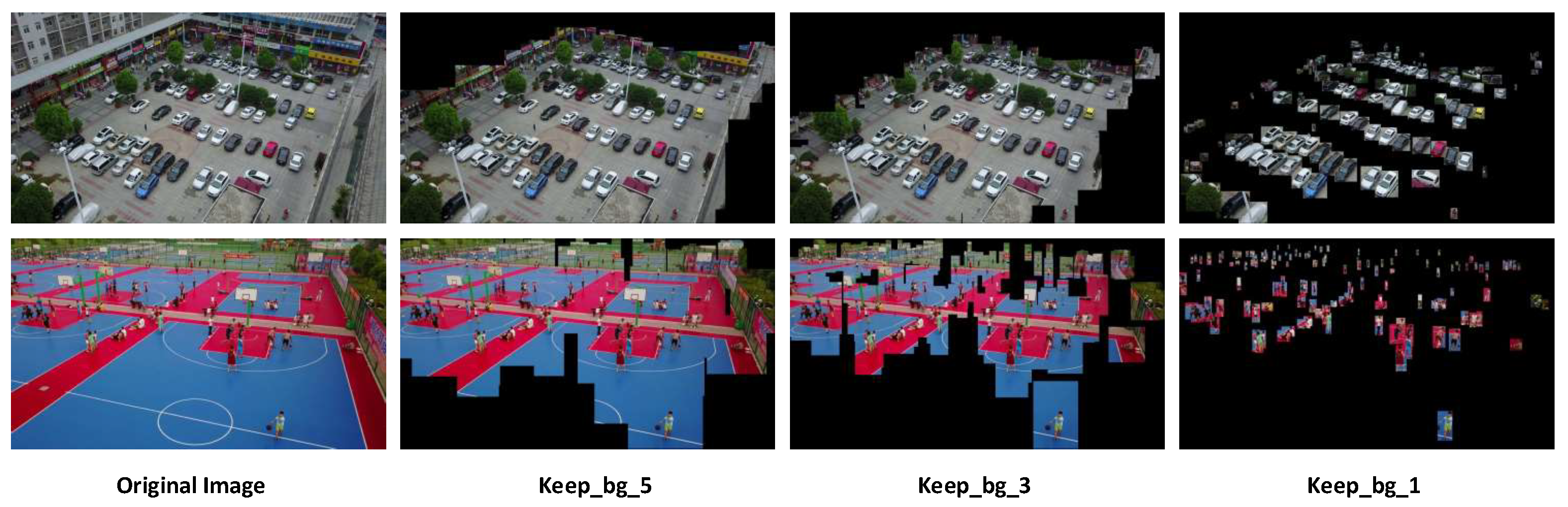
13], which cause the destruction of object detection context. However, feature pyramid networks in this paper use the whole image to train, thus avoiding the same problem. In this section, to study the influences of background context on object detection, we conducted a simple comparative experiment. Based on a RetinaNet trained on the original image, part of the background in the test images was then removed to study the object detection model’s performance changes. Some experimental pictures are shown in Figure 8.
From the results of Table 1, it can be seen that after cropping the background area around the target in the original image, it has a significant impact on various metric indicators. As the cropping area decreases, the performance gradually recovers. However, even if it retains five times the background area around the objects (as shown in the second column of Figure 8) still weakens the detection performance. Therefore, a series of image pyramids based on image region slices nearly destroy the object detection context and cannot achieve optimal performance.
In Table 2, we conducted an experiment to pointed out the impact of image size changes on detection performance. All images are scaled to a size of 512 × 512 during training the network. Next, in the inference stage, the input images are enlarged or reduced to be tested by the trained model. It can be seen that the mean average accuracy (mAP) of the network trained in the size of 512 × 512 is 0.111, which indicates the overall performance of the detector. As the input images shrink, the mAP gradually decreases, and when the images are enlarged, the mAP increases by 0.032 in absolute value (over 28.8%) at most.
The overall improvement mainly comes from the improvement of medium and small objects. When the image is enlarged, the detection performance of large objects decreases. When the network was retrained at the image size of 1024 × 1024 , mAP increased by 0.106 (more than 95.4%), and various indicators such as AP_small, AP_medium, and AP_large were significantly improved. Therefore, it can be concluded that compared with the training image size of 512 × 512 , proper image magnification can greatly improve the performance of various indicators of object detection. From the visualized feature map in Figure 9, it can also be seen that the feature maps of enlarged image have a sharper activation area for small and medium objects, which are easier to achieve higher accuracy in subsequent positioning and recognition steps.

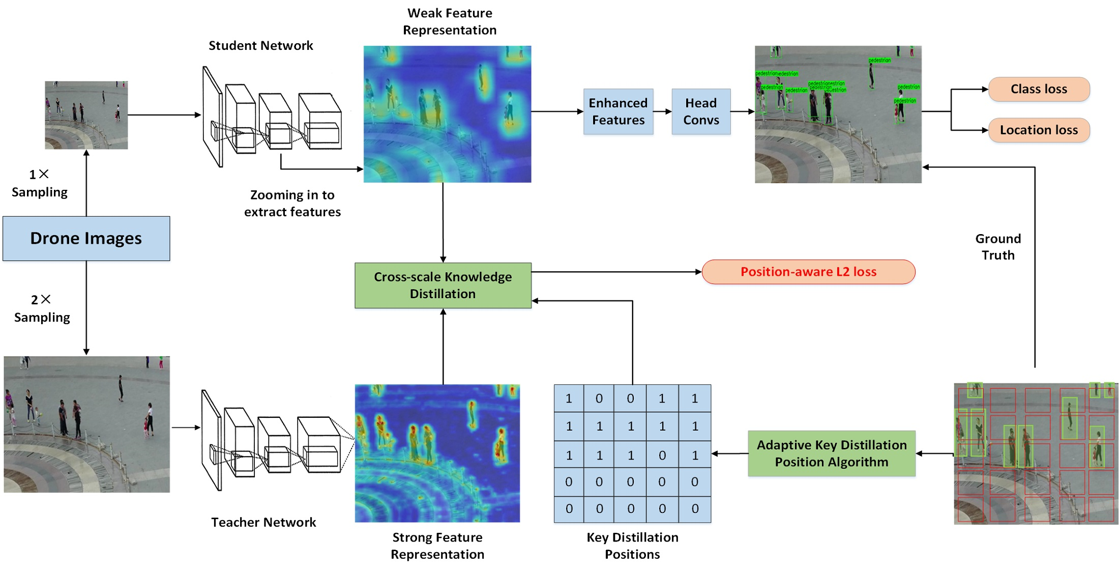
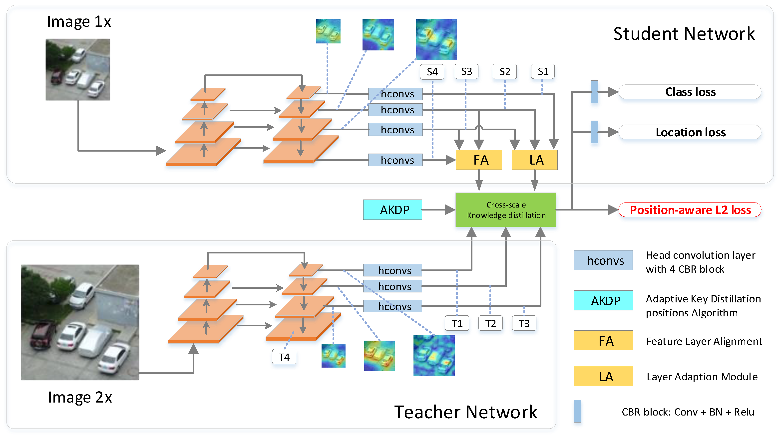
3.5.2. Results of Cross-Scale Knowledge Distillation

We trained the student network (SNet) with the original input images, and trained the teacher network (TNet) with the input of two times the size. In Table 3, we carried out detailed ablation experiments by gradually adding structures such as layer adaption (LA) and feature layer alignment (FA), and then carried out cross-scale knowledge distillation (CSKD) via adaptive key distillation positions (AKDP) algorithm. For each network with added structure, we compared the changes of calculation and accuracy, in which the amount of calculation was measured by Giga Floating-point Operations Per Second (GFLOPs).
It can be seen in Table 3 that TNet has the highest performance, but its calculation amount is four times that of SNet, which is difficult to apply in the actual environment. Directly performing knowledge distillation on SNet (subsampling the feature map of the teacher model) can only get a 0.005 (4.5%) mAP improvement, and it can be seen from the A P _ S (0.028) that direct distillation without any additional component has no effect on the detection performance of small objects.
After introducing LA, mAP has increased by 0.014 (12.61%) compared with SNet, and A P _ S has almost doubled (92.85%), indicating that the LA structure we introduced is effective especially for small objects. After the CSKD of the SNet with the layer adaptive structure, the mAP continues to increase to 21.62%, indicating that the introduction structure is conducive to better knowledge distillation. At the same time, by comparing the amount of calculation, it is found that compared with the SNet with 53.3 GFLOPs of calculation consumption, the introduction of LA only brings the calculation of SNet to 58.05 GFLOPs, which only increases by 8.9%.
Because the LA structure only aligns the output size of the two models through upsampling forcibly, the inputs of SNet and TNet are still different, which influences the effectiveness of CSKD. Furthermore, we introduce the FA mechanism to align the feature level, and the mAP is raised from 0.111 to 0.15 (35.13%), and to 0.162 (45.94%) after CSKD, but it also brings a huge increase in computational complexity. This is because the output feature map of the network continues to be convoluted by four layers in RetinaNet, and then the categories and locations of the objects are predicted. The convolution of these four layers leads to a sharp increase in the amount of computation after the introduction of FA. We conducted a comparative experiment using only two-layer convolution (SNet+FA_ThinHead). It is found that after reducing the two-layer convolution, the amount of computation is reduced from 146.09 GFLOPs to 94.56 GFLOPs (35.27%). However, the simplified FA method still increases the mAP from 0.111 to 0.140 (26.13%) and to 0.142 (27.93%) after CSKD, which shows the effectiveness of the FA structure. The amount of computation brought by the FA structure can be optimized by simplifying the subsequent convolution layer of the output feature map. In fact, it can be optimized by the BottleNeck structure used in ResNet [26] or the depthwise separable convolution used in MobileNet [43], but it is not the focus of this paper. Here, we only discuss the effectiveness and good optimizability of CSKD based on FA structure.

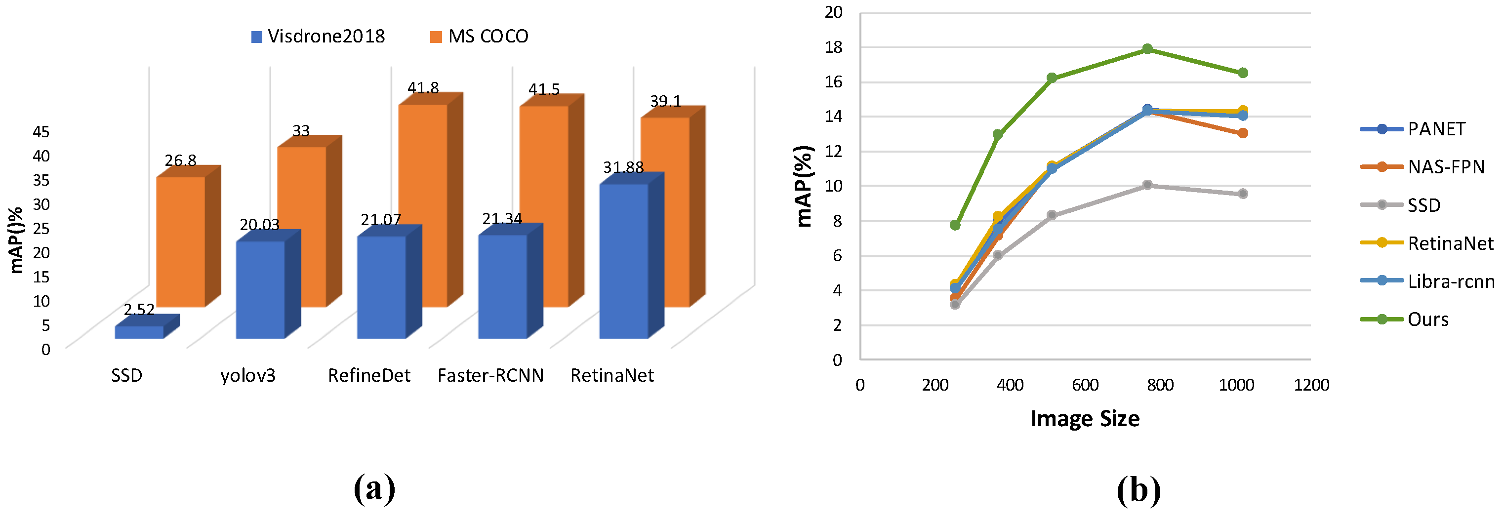
3.5.3. Comparison to the SOTA FPNs

In Table 4, we compare the large, medium, and small object detection accuracy (AP_S/AP_M/AP_L); recall rate (AR_S/AR_M/AR_L); and mAP with five SOTA feature pyramid methods under unified conditions. Note that Ours-FA_CSKD_th is the same as SNet with FA_ThinHead and CSKD.
Due to the direct use of each feature level for prediction without fusion of shallow and deep features, all metrics of SSD are the worst. Compared with SSD, FPN, PAFPN, NAS-FPN, and Libra-RCNN use different methods for feature fusion, and all indicators have been improved. However, it can be seen that the performance of these methods is very close, which shows that it is difficult to get a more robust feature representation of small objects by relying solely on the feature pyramid fusion.
Based on the most basic feature pyramid structure, we introduced LA, FA, and CSKD strategy, the average detection accuracy has been significantly improved. Because the teacher network in our CSKD architecture is trained by enlarged images, the improvement mainly comes from small and medium-sized objects. It can see that our method exceeds five networks in AP_S, AP_M, AR_S, and AR_M. Among them, LA_CSKD is the lightest version, whose results of mAP, AP_S, AP_M, AR_S, and AR_M are increased by 21.62%, 106.89%, 10.82%, 64.17%, and 12.54%, respectively, compared to SNet.
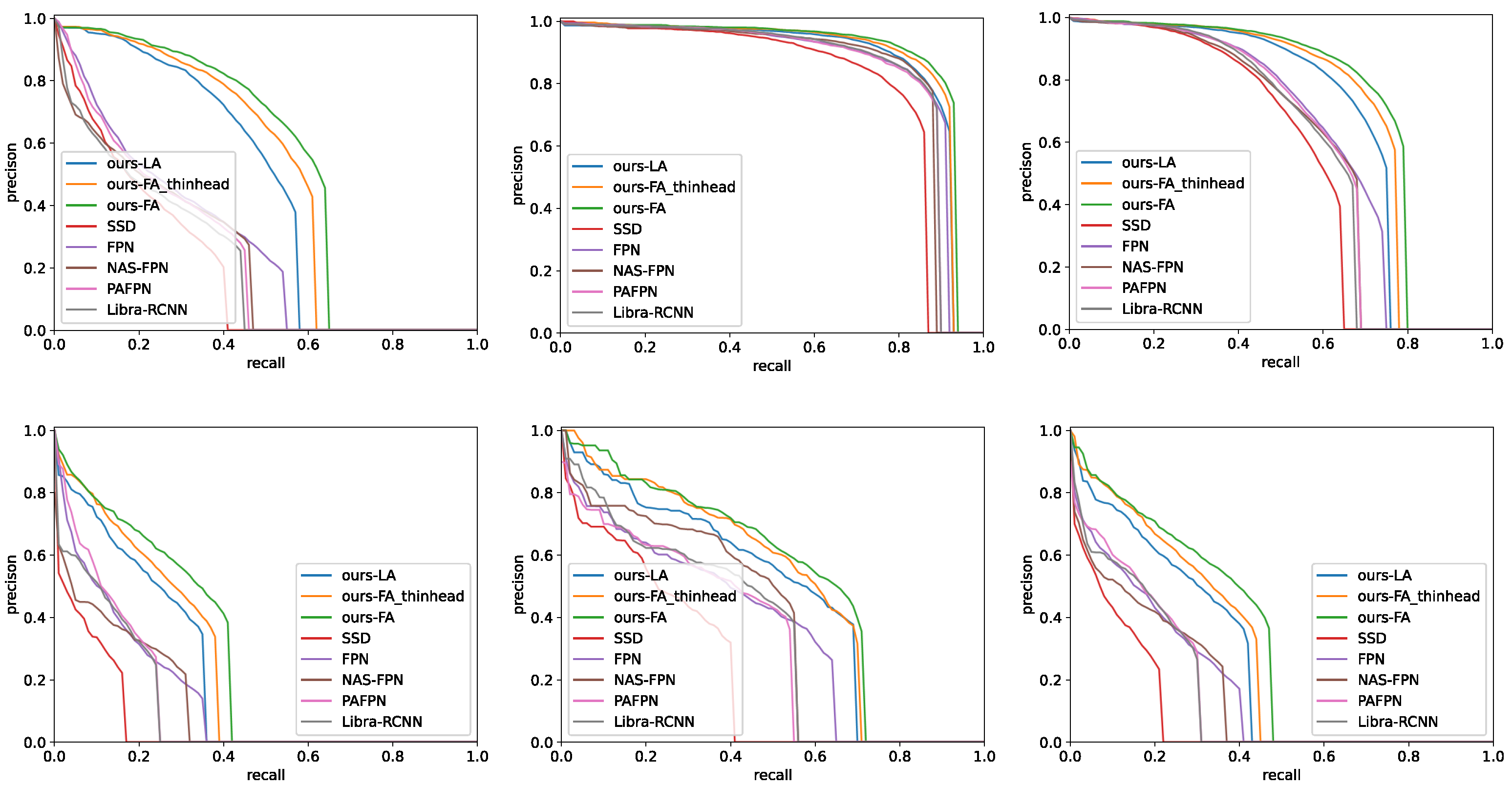
Figure 10 shows the precision–recall (PR) curves of medium, small, and all objects. At the same recall point, the higher the accuracy, the better the model performance. It can be seen that all versions of our method are better than the other five methods in the performance of small and medium objects (Figure 10a,b), especially the small objects, making the overall performance (Figure 10c) better than other methods.
In comparing the average accuracy of each category in Table 5, we can see that the sample imbalance and size imbalance lead to differences in accuracy. Categories of car, van, and bus with larger sizes have the better average accuracy, while small object categories such as people and pedestrian have worse accuracy. Our proposed approach is superior to the other five mainstream methods in most categories (except truck and awning-tricycle).
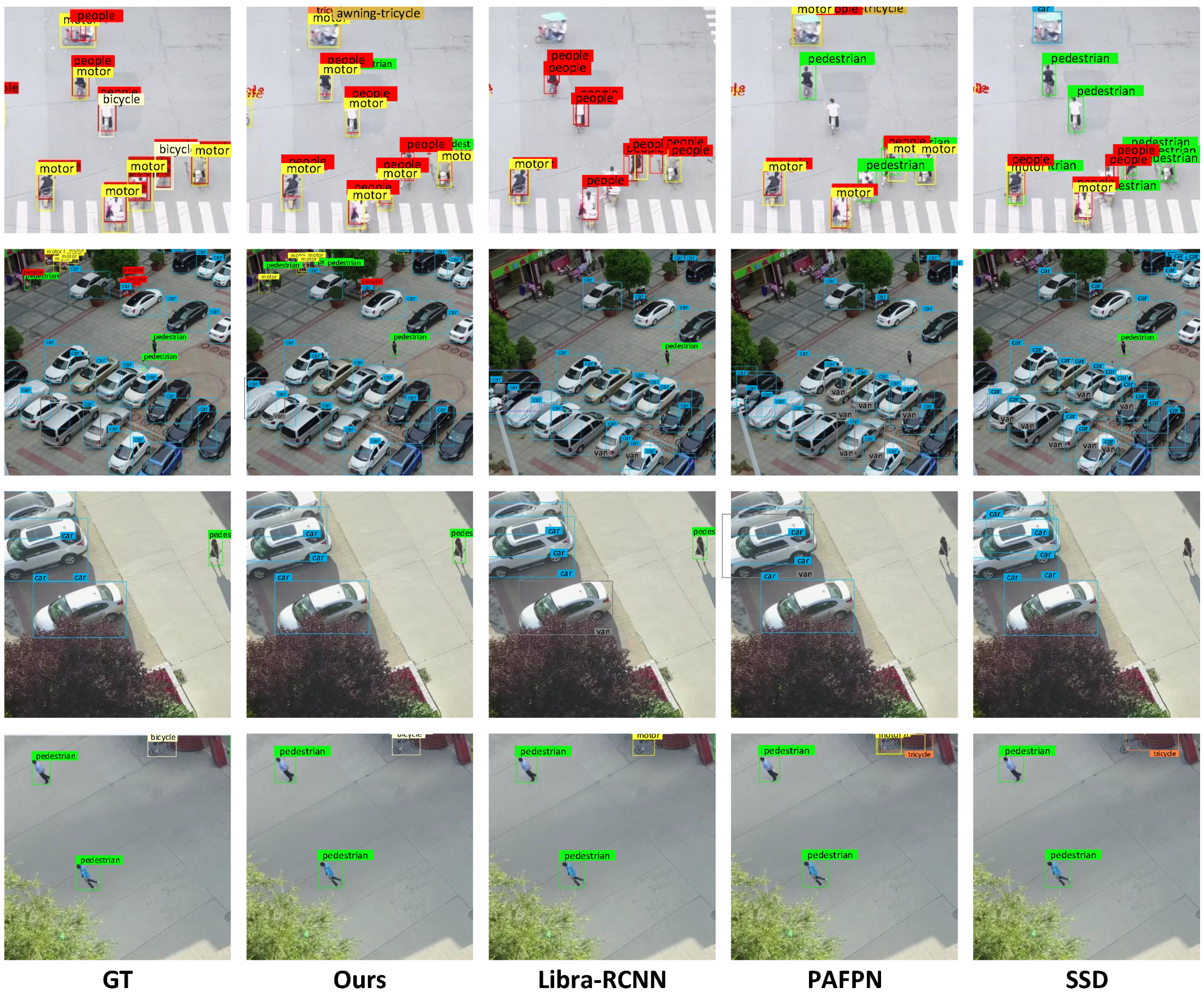
The first row in Figure 11 shows a difficult situation in the visdrone2018 dataset. People sitting in motors are highly overlapping, but they need to be accurately divided into two categories: people (red) and motor (yellow). It can be seen that Libra-RCNN, PAFPN and SSD almost all missed or misclassified these two categories of objects, while our results have only a few errors. Among them, the green border is a pedestrian. The difference between a pedestrian and a person is that the former is standing and the latter is sitting.
In the second row, several motors and pedestrians in the image have only weak feature representation. Our ZoomInNet successfully detected some of them, while other methods missed all of them. The third and fourth rows are similar, our method always outperforms other methods in detecting small objects.

3.5.4. Comparison to the SOTAs in VisDrone-DET2019

Note that the small detection accuracy is still low in this paper and mAPs of our method are lower than ones of these SOTA reported in VisDrone-DET2019 [44]. In this section, we conducted experiments to explain the “low accuracy” in this paper. The main reason is that the experiments above are conducted under uniform conditions without additional accessories.
In fact, both VisDrone-DET2018 [10] and VisDrone-DET2019 are data challenges, which means that any technique or trick can be used for improving the results. Such tricks include data augmentation, deeper backbone network, larger image size and technique in training or inference stages. For example, among the 33 methods represented by A.1–A.33 in VisDrone-DET2019, backbones of ResNet-101 [26], ResNeXt-101 [45], and ResNet-50 [26] are used in methods A.1–A.3, respectively; a guide anchor [46] is used in A.2 for training; Test time augmentation (TTA) and Soft-NMS [47] are used for inference in A.13.
In Table 6, we show that with several tricks, even the baseline of our method can achieve results similar to those reported in VisDrone-DET2019.
It can be seen that with some tricks, the mAP results of our baseline have greatly improved from 11.1% to 28.0%, while the AP_S also rise from 2.8% to 19.2%. Among the six compared methods, DPNet-ensemble (A.15) has the best mAP in [44]. Without any efficiency optimization, our method roughly uses some tricks, but still achieves a moderate speed with a TITAN RTX 24G. However, the speed of our baseline decreased from 27.8 to 3.9 FPS. Therefore, methods with many tricks in [44] are hard to apply in real environment. Furthermore, while comparing CSKD with FPNs, the tricks such as multi-scale training or inference become interfering factors. Base on the above analysis, we eliminated all the tricks used in [44].
To compare the methods in VisDrone-DET2019, we must implement them under unified framework and experimental conditions. Therefore, the detection models mainly involved in 33 algorithms in VisDrone-DET2019 are counted as shown in Table 7.
According to the statistical results in Table 7, the number of occurrences of top 6 detectors accounted for 83.3% among the 12 detectors, where RetinaNet and Libra-RCNN have already compared in Section 3.5.3. For CenterNet, it has no pre-implemented model in the MMDetection [42] framework. Therefore, we conducted further comparison with Cascade-RCNN, Faster RCNN (FR) with HRNet and Faster RCNN with ResNet-50. The results are shown in Table 8.
It can be seen that under uniform conditions, our method is better than the three most commonly used methods in [44] in AP and AR of small objects. Our results on medium and large objects are slightly worse than other methods. This is because we use the small-scale images to train the student network and the large-scale images to train the teacher network. Therefore, what we improve is the detection performance of small objects, but maybe the detection performance of medium and large objects can also be improved with CSKD, which is also the direction of our future work.

3.5.5. Comparison to Fine-Tuning Method

In this paper, we proposed to use CSKD for utilizing the advantages of network trained by large-scale images, while fine-tuning is the other method can achieve the similar purpose. Therefore, in this section, we conducted comparison to the fine-tuning method for further demonstration of the effectiveness of CSKD. To explore it, we pre-trained the baseline using double size images (1024 × 1024) for 20 epochs, which is the same as TNet in Table 3, and then fine-tuned the network using the original size images (512 × 512) for 10 epochs. There are two ways to set the fine-tune learning rate (LR) in our experiments:
  • keep the same as the 20th epoch and set to 0.1 times the previous after 3 epochs
  • set to 0.1 times the previous at the beginning of fine-tuning
The first setting way considers keeping the LR consistent with the pre-training to keep the initial fine-tuning smooth, and after a few epochs, it becomes smaller to help the model converge to a higher accuracy. The second setting method considers the large difference in image input between pre-training and fine-tuning. In the initial stage of fine-tuning, a smaller learning rate is required to avoid shocks. The results are shown in Table 9.
With the network pretrained with image size of 1024 × 1024, the mAP obtained by inference under image size of 512 × 512 is 11.7%, which drops a lot compared to inference result under image size of 1024 × 1024 (21.7%), but is still better than the network with image size of 512 × 512 for both training and inference (11.1%). This shows that pre-training at a large size is helpful to improve mAP.
The fine-tuning methods with two LR setting ways can slightly improve the results of mAP, while have almost no influences on the average accuracy and recall rate of small objects. This is consistent with the ablation study in Table 3. The experiment “SNet + CSKD” shows that without changing the model structure, CSKD also obtained weak effect on mAP and AP_S. After the introduction of LA, the mAP and AP_S have been significantly improved.
In this paper, we aim to use cross-scale models for improving the performance of small objects, and the two most critical points are that
  • the training of small-scale model (SSM) should be guided by the knowledge of large-scale model (LSM) and
  • there should be corresponding structures in SSM to maintain knowledge of LSM.
For the fine-tuning method, the huge change in the image size leads to the huge change in the features, which in turn leads to a sharp drop in the model performance during the fine-tuning process. This is because the cross-scale fine-tuning lacks supervised guidance, and the SSM cannot retain the knowledge learned in the LSM. In contrast, our method uses knowledge distillation to play the guiding role of LSM to SSM, and at the same time maintains cross-scale knowledge through two improved structures of LA and FA, which achieve better results.

4. Conclusions

In this paper, we have drawn on the advantages of image pyramid methods for enhancing the feature representation of small objects, and proposed a cross-scale knowledge distillation (CSKD) architecture to compress cross-scale information into a single model. The experiments conducted on VisDrone-DET2018 challenging dataset demonstrate that the proposed LA and FA mechanism can help better CSKD, which improve the performance of small objects detection significantly. Based on the basic feature pyramid structure, our ZoomInNet achieves higher accuracy in small objects detection compared to five SOTA feature pyramid methods.
By comparative experiments with methods in VisDrone-DET2019, we show that with some tricks, even our baseline can achieve a high accuracy as reported in VisDrone-DET2019. Without these tricks, the comparison with SOTA in VisDrone-DET2019 shows that our method can give better results for small object detection.
The comparison with the fine-tuning method further proves that CSKD proposed in this paper can effectively utilize the cross-scale model to improve the performance of small object detection.

Author Contributions

B.-Y.L. proposed the frameworks and conducted the experiments. H.-X.C. and Y.-Z.Y. provided suggestions and reviewed the manuscript. Z.H. wrote the manuscript together with B.-Y.L. and reviewed the manuscript; X.L. curated the data. All authors have read and agreed to the published version of the manuscript.

Funding

This research was funded by Sichuan Major Science and Technology Special Project grant number 2018GZDZX0017.

Data Availability Statement

All the drone data used in this paper is from Visdrone Challenge, which can be found in http://aiskyeye.com/ (accessed on 6 February 2021).

Conflicts of Interest

The authors declare no conflict of interest.

References

  1. Tang, L.; Shao, G. Drone remote sensing for forestry research and practices. J. For. Res. 2015, 26, 791–797. [Google Scholar] [CrossRef]
  2. Bansod, B.; Singh, R.; Thakur, R.; Singhal, G. A comparision between satellite based and drone based remote sensing technology to achieve sustainable development: A review. J. Agric. Environ. Int. Dev. JAEID 2017, 111, 383–407. [Google Scholar]
  3. Gray, P.C.; Ridge, J.T.; Poulin, S.K.; Seymour, A.C.; Schwantes, A.M.; Swenson, J.J.; Johnston, D.W. Integrating drone imagery into high resolution satellite remote sensing assessments of estuarine environments. Remote Sens. 2018, 10, 1257. [Google Scholar] [CrossRef] [Green Version]
  4. Pinggera, P.; Ramos, S.; Gehrig, S.; Franke, U.; Rother, C.; Mester, R. Lost and found: Detecting small road hazards for self-driving vehicles. In Proceedings of the 2016 IEEE/RSJ International Conference on Intelligent Robots and Systems, Daejeon, Korea, 9–14 October 2016; IEEE: Piscataway, NJ, USA, 2016; pp. 1099–1106. [Google Scholar]
  5. Houben, S.; Stallkamp, J.; Salmen, J.; Schlipsing, M.; Igel, C. Detection of traffic signs in real-world images: The German Traffic Sign Detection Benchmark. In Proceedings of the 2013 International Joint Conference on Neural Networks, Dallas, TX, USA, 4–6 August 2013; IEEE: Piscataway, NJ, USA, 2013; pp. 1–8. [Google Scholar]
  6. Mueller, M.; Smith, N.; Ghanem, B. A benchmark and simulator for uav tracking. In Proceedings of the European Conference on Computer Vision, Amsterdam, The Netherlands, 11–14 October 2016; Springer: Berlin/Heidelberg, Germany, 2016; pp. 445–461. [Google Scholar]
  7. Du, D.; Qi, Y.; Yu, H.; Yang, Y.; Duan, K.; Li, G.; Zhang, W.; Huang, Q.; Tian, Q. The unmanned aerial vehicle benchmark: Object detection and tracking. In Proceedings of the European Conference on Computer Vision, Munich, Germany, 8–14 September 2018; Springer: Berlin/Heidelberg, Germany, 2018; pp. 370–386. [Google Scholar]
  8. Lin, T.Y.; Maire, M.; Belongie, S.; Hays, J.; Perona, P.; Ramanan, D.; Dollár, P.; Zitnick, C.L. Microsoft coco: Common objects in context. In Proceedings of the European Conference on Computer Vision, Zurich, Switzerland, 6–12 September 2014; Springer: Berlin/Heidelberg, Germany, 2014; pp. 740–755. [Google Scholar]
  9. Russakovsky, O.; Deng, J.; Su, H.; Krause, J.; Satheesh, S.; Ma, S.; Huang, Z.; Karpathy, A.; Khosla, A.; Bernstein, M.; et al. Imagenet large scale visual recognition challenge. Int. J. Comput. Vis. 2015, 115, 211–252. [Google Scholar] [CrossRef] [Green Version]
  10. Zhu, P.; Wen, L.; Du, D.; Bian, X.; Ling, H.; Hu, Q.; Nie, Q.; Cheng, H.; Liu, C.; Liu, X.; et al. Visdrone-det2018: The vision meets drone object detection in image challenge results. In Proceedings of the European Conference on Computer Vision Workshops, Munich, Germany, 8–14 September 2018. [Google Scholar]
  11. Singh, B.; Davis, L.S. An analysis of scale invariance in object detection snip. In Proceedings of the IEEE Conference on Computer Vision and Pattern Recognition, Salt Lake City, UT, USA, 18–22 June 2018; IEEE: Piscataway, NJ, USA, 2018; pp. 3578–3587. [Google Scholar]
  12. Singh, B.; Najibi, M.; Davis, L.S. Sniper: Efficient multi-scale training. arXiv 2018, arXiv:1805.09300. [Google Scholar]
  13. Najibi, M.; Singh, B.; Davis, L.S. Autofocus: Efficient multi-scale inference. In Proceedings of the IEEE/CVF International Conference on Computer Vision, Seoul, Korea, 27–28 October 2019; IEEE: Piscataway, NJ, USA, 2019; pp. 9745–9755. [Google Scholar]
  14. Liu, W.; Anguelov, D.; Erhan, D.; Szegedy, C.; Reed, S.; Fu, C.Y.; Berg, A.C. Ssd: Single shot multibox detector. In Proceedings of the European Conference on Computer Vision, Amsterdam, The Netherlands, 11–14 October 2016; Springer: Berlin/Heidelberg, Germany, 2016; pp. 21–37. [Google Scholar]
  15. Farhadi, A.; Redmon, J. Yolov3: An incremental improvement. arXiv 2018, arXiv:1804.02767. [Google Scholar]
  16. Ren, S.; He, K.; Girshick, R.; Sun, J. Faster r-cnn: Towards real-time object detection with region proposal networks. arXiv 2015, arXiv:1506.01497. [Google Scholar] [CrossRef] [PubMed] [Green Version]
  17. Lin, T.Y.; Goyal, P.; Girshick, R.; He, K.; Dollár, P. Focal loss for dense object detection. In Proceedings of the IEEE International Conference on Computer Vision, Venice, Italy, 22–29 October 2017; IEEE: Piscataway, NJ, USA, 2017; pp. 2980–2988. [Google Scholar]
  18. Liu, S.; Qi, L.; Qin, H.; Shi, J.; Jia, J. Path aggregation network for instance segmentation. In Proceedings of the IEEE Conference on Computer Vision and Pattern Recognition, Salt Lake City, UT, USA, 18–22 June 2018; IEEE: Piscataway, NJ, USA, 2018; pp. 8759–8768. [Google Scholar]
  19. Ghiasi, G.; Lin, T.Y.; Le, Q.V. Nas-fpn: Learning scalable feature pyramid architecture for object detection. In Proceedings of the IEEE/CVF Conference on Computer Vision and Pattern Recognition, Long Beach, CA, USA, 15–20 June 2019; IEEE: Piscataway, NJ, USA, 2019; pp. 7036–7045. [Google Scholar]
  20. Pang, J.; Chen, K.; Shi, J.; Feng, H.; Ouyang, W.; Lin, D. Libra r-cnn: Towards balanced learning for object detection. In Proceedings of the IEEE/CVF Conference on Computer Vision and Pattern Recognition, Long Beach, CA, USA, 15–20 June 2019; IEEE: Piscataway, NJ, USA, 2019; pp. 821–830. [Google Scholar]
  21. Bell, S.; Zitnick, C.L.; Bala, K.; Girshick, R. Inside-outside net: Detecting objects in context with skip pooling and recurrent neural networks. In Proceedings of the IEEE Conference on Computer Vision and Pattern Recognition, Las Vegas, NV, USA, 27–30 June 2016; IEEE: Piscataway, NJ, USA, 2016; pp. 2874–2883. [Google Scholar]
  22. Lin, T.Y.; Dollár, P.; Girshick, R.; He, K.; Hariharan, B.; Belongie, S. Feature pyramid networks for object detection. In Proceedings of the IEEE Conference on Computer Vision and Pattern Recognition, Honolulu, HI, USA, 21–26 July 2017; IEEE: Piscataway, NJ, USA, 2017; pp. 2117–2125. [Google Scholar]
  23. Hinton, G.; Vinyals, O.; Dean, J. Distilling the knowledge in a neural network. arXiv 2015, arXiv:1503.02531. [Google Scholar]
  24. Phuong, M.; Lampert, C. Towards understanding knowledge distillation. In Proceedings of the International Conference on Machine Learning, Long Beach, CA, USA, 9–15 June 2019; International Machine Learning Society (IMLS): Stroudsburg, PA, USA, 2019; pp. 5142–5151. [Google Scholar]
  25. Mirzadeh, S.I.; Farajtabar, M.; Li, A.; Levine, N.; Matsukawa, A.; Ghasemzadeh, H. Improved knowledge distillation via teacher assistant. In Proceedings of the AAAI Conference on Artificial Intelligence, New York, NY, USA, 7–12 February 2020; Volume 34, pp. 5191–5198. [Google Scholar]
  26. He, K.; Zhang, X.; Ren, S.; Sun, J. Deep residual learning for image recognition. In Proceedings of the IEEE Conference on Computer Vision and Pattern Recognition, Las Vegas, NV, USA, 27–30 June 2016; IEEE: Piscataway, NJ, USA, 2016; pp. 770–778. [Google Scholar]
  27. Girshick, R. Fast r-cnn. In Proceedings of the IEEE International Conference on Computer Vision, Santiago, Chile, 7–13 December 2015; IEEE: Piscataway, NJ, USA, 2015; pp. 1440–1448. [Google Scholar]
  28. Chen, Z.; Wu, K.; Li, Y.; Wang, M.; Li, W. SSD-MSN: An Improved Multi-Scale Object Detection Network Based on SSD. IEEE Access 2019, 7, 80622–80632. [Google Scholar] [CrossRef]
  29. Chen, G.; Choi, W.; Yu, X.; Han, T.; Chandraker, M. Learning efficient object detection models with knowledge distillation. In Proceedings of the 31st International Conference on Neural Information Processing Systems, Long Beach, CA, USA, 4–9 December 2017; NIPS: La Jolla, CA, USA, 2017; pp. 742–751. [Google Scholar]
  30. Xu, K.; Rui, L.; Li, Y.; Gu, L. Feature Normalized Knowledge Distillation for Image Classification. In Proceedings of the European Conference on Computer Vision, SEC, Glasgow, British, 23–28 August 2020; Springer: Berlin/Heidelberg, Germany, 2018; Volume 1. [Google Scholar]
  31. Liu, Y.; Sheng, L.; Shao, J.; Yan, J.; Xiang, S.; Pan, C. Multi-label image classification via knowledge distillation from weakly-supervised detection. In Proceedings of the 26th ACM International Conference on Multimedia, Gothenburg, Sweden, 27–28 May 2018; IEEE: Piscataway, NJ, USA, 2018; pp. 700–708. [Google Scholar]
  32. Chen, W.C.; Chang, C.C.; Lee, C.R. Knowledge distillation with feature maps for image classification. In Proceedings of the Asian Conference on Computer Vision, Perth, Australia, 2–6 December 2018; Springer: Berlin/Heidelberg, Germany, 2018; pp. 200–215. [Google Scholar]
  33. Liu, Y.; Chen, K.; Liu, C.; Qin, Z.; Luo, Z.; Wang, J. Structured knowledge distillation for semantic segmentation. In Proceedings of the IEEE/CVF Conference on Computer Vision and Pattern Recognition, Long Beach, CA, USA, 15–20 June 2019; IEEE: Piscataway, NJ, USA, 2019; pp. 2604–2613. [Google Scholar]
  34. Dou, Q.; Liu, Q.; Heng, P.A.; Glocker, B. Unpaired multi-modal segmentation via knowledge distillation. IEEE Trans. Med. Imaging 2020, 39, 2415–2425. [Google Scholar] [CrossRef] [PubMed] [Green Version]
  35. Michieli, U.; Zanuttigh, P. Knowledge distillation for incremental learning in semantic segmentation. Comput. Vis. Image Underst. 2021, 205, 103167. [Google Scholar] [CrossRef]
  36. Zhang, P.; Su, L.; Li, L.; Bao, B.; Cosman, P.; Li, G.; Huang, Q. Training Efficient Saliency Prediction Models with Knowledge Distillation. In Proceedings of the 27th ACM International Conference on Multimedia, Montreal, QC, Canada, 25–26 May 2019; IEEE: Piscataway, NJ, USA, 2019; pp. 512–520. [Google Scholar]
  37. Huang, Z.; Chen, H.X.; Zhou, T.; Yang, Y.Z.; Wang, C.Y.; Liu, B.Y. Contrast-weighted dictionary learning based saliency detection for VHR optical remote sensing images. Pattern Recognit. 2020, 113, 107757. [Google Scholar] [CrossRef]
  38. Huang, Z.; Chen, H.X.; Zhou, T.; Yang, Y.Z.; Wang, C.Y. Multi-level cross-modal interaction network for RGB-D salient object detection. arXiv 2020, arXiv:2007.14352. [Google Scholar]
  39. Wang, T.; Yuan, L.; Zhang, X.; Feng, J. Distilling object detectors with fine-grained feature imitation. In Proceedings of the IEEE/CVF Conference on Computer Vision and Pattern Recognition, Long Beach, CA, USA, 15–20 June 2019; IEEE: Piscataway, NJ, USA, 2019; pp. 4933–4942. [Google Scholar]
  40. Ioffe, S.; Szegedy, C. Batch normalization: Accelerating deep network training by reducing internal covariate shift. In Proceedings of the International Conference on Machine Learning, Lile, France, 6–11 July 2015; ICML: Stroudsburg, PA, USA, 2015; pp. 448–456. [Google Scholar]
  41. Glorot, X.; Bordes, A.; Bengio, Y. Deep sparse rectifier neural networks. In Proceedings of the 14th International Conference on Artificial Intelligence and Statistics, JMLR Workshop and Conference Proceedings, Chung-Li, Taiwan, 11–13 November 2011; IEEE: Piscataway, NJ, USA, 2011; pp. 315–323. [Google Scholar]
  42. Chen, K.; Wang, J.; Pang, J.; Cao, Y.; Xiong, Y.; Li, X.; Sun, S.; Feng, W.; Liu, Z.; Xu, J.; et al. MMDetection: Open mmlab detection toolbox and benchmark. arXiv 2019, arXiv:1906.07155. [Google Scholar]
  43. Howard, A.G.; Zhu, M.; Chen, B.; Kalenichenko, D.; Wang, W.; Weyand, T.; Andreetto, M.; Adam, H. Mobilenets: Efficient convolutional neural networks for mobile vision applications. arXiv 2017, arXiv:1704.04861. [Google Scholar]
  44. Du, D.; Zhu, P.; Wen, L.; Bian, X.; Lin, H.; Hu, Q.; Peng, T.; Zheng, J.; Wang, X.; Zhang, Y.; et al. VisDrone-DET2019: The Vision Meets Drone Object Detection in Image Challenge Results. In Proceedings of the IEEE/CVF International Conference on Computer Vision (ICCV) Workshops, Seoul, Korea, 27 October–2 November 2019. [Google Scholar]
  45. Xie, S.; Girshick, R.; Dollár, P.; Tu, Z.; He, K. Aggregated residual transformations for deep neural networks. In Proceedings of the IEEE Conference on Computer Vision and Pattern Recognition, Honolulu, HI, USA, 21–26 July 2017; IEEE: Piscataway, NJ, USA, 2017; pp. 1492–1500. [Google Scholar]
  46. Wang, J.; Chen, K.; Yang, S.; Loy, C.C.; Lin, D. Region proposal by guided anchoring. In Proceedings of the IEEE/CVF Conference on Computer Vision and Pattern Recognition, Long Beach, CA, USA, 15–20 June 2019; IEEE: Piscataway, NJ, USA, 2019; pp. 2965–2974. [Google Scholar]
  47. Bodla, N.; Singh, B.; Chellappa, R.; Davis, L.S. Soft-NMS–improving object detection with one line of code. In Proceedings of the IEEE International Conference on Computer Vision, Venice, Italy, 22–29 October 2017; IEEE: Piscataway, NJ, USA, 2017; pp. 5561–5569. [Google Scholar]
  48. Cai, Z.; Vasconcelos, N. Cascade r-cnn: Delving into high quality object detection. In Proceedings of the IEEE Conference on Computer Vision and Pattern Recognition, Salt Lake City, UT, USA, 18–22 June 2018; IEEE: Piscataway, NJ, USA, 2018; pp. 6154–6162. [Google Scholar]
  49. Zhou, X.; Wang, D.; Krähenbühl, P. Objects as points. arXiv 2019, arXiv:1904.07850. [Google Scholar]
  50. Sun, K.; Xiao, B.; Liu, D.; Wang, J. Deep high-resolution representation learning for human pose estimation. In Proceedings of the IEEE/CVF Conference on Computer Vision and Pattern Recognition, Long Beach, CA, USA, 15–20 June 2019; IEEE: Piscataway, NJ, USA, 2019; pp. 5693–5703. [Google Scholar]
  51. Yu, C.; Wang, J.; Peng, C.; Gao, C.; Yu, G.; Sang, N. Learning a discriminative feature network for semantic segmentation. In Proceedings of the IEEE Conference on Computer Vision and Pattern Recognition, Salt Lake City, UT, USA, 18–22 June 2018; IEEE: Piscataway, NJ, USA, 2018; pp. 1857–1866. [Google Scholar]
  52. Cheng, Z.; Wu, Y.; Xu, Z.; Lukasiewicz, T.; Wang, W. Segmentation is All You Need. arXiv 2019, arXiv:1904.13300. [Google Scholar]
  53. Li, Y.; Chen, Y.; Wang, N.; Zhang, Z. Scale-aware trident networks for object detection. In Proceedings of the IEEE/CVF International Conference on Computer Vision, Seoul, Korea, 27 October–2 November 2019; IEEE: Piscataway, NJ, USA, 2019; pp. 6054–6063. [Google Scholar]
  54. He, K.; Gkioxari, G.; Dollár, P.; Girshick, R. Mask r-cnn. In Proceedings of the IEEE International Conference on Computer Vision, Venice, Italy, 22–29 October 2017; IEEE: Piscataway, NJ, USA, 2017; pp. 2961–2969. [Google Scholar]
  55. Chen, K.; Pang, J.; Wang, J.; Xiong, Y.; Li, X.; Sun, S.; Feng, W.; Liu, Z.; Shi, J.; Ouyang, W.; et al. Hybrid task cascade for instance segmentation. In Proceedings of the IEEE/CVF Conference on Computer Vision and Pattern Recognition, Long Beach, CA, USA, 15–20 June 2019; IEEE: Piscataway, NJ, USA, 2019; pp. 4974–4983. [Google Scholar]
Figure 2. Two kinds of pyramid method for handling multi-scale problem in object detection. (a) Image Pyramid uses multi-scale images for prediction. (b) Feature Pyramid uses different levels in the feature extraction process for prediction.
Remotesensing 13 01198 g002
Figure 3. Cross-scale knowledge distillation architecture of proposed ZoomInNet. The feature maps from teacher and student networks are aligned via LA and FA mechanism, and then AKDP algorithm is used to calculate the key positions at feature maps, the position-aware L2 loss is used to measure the difference between feature maps from the teacher and student models.
Remotesensing 13 01198 g003
Figure 4. A 3 × 3 input is filled and processed by the 3 × 3 CBR module.
Remotesensing 13 01198 g004
Figure 5. The Adaptive Key Distillation Positions (AKDP) Algorithm for anchor-based feature map distillation. In the first step, feature mask is computed based on the IOU between the preset anchors and true bounding boxes, which indicates the attention area in both teacher’s and student’s feature map. Then, the position-aware L2 distance is used to measure the gap between the teacher-network and student-network.
Remotesensing 13 01198 g005
Figure 6. Some images in Visdrone2018 dataset. The angle, scale and illumination changes, and dense small objects in this dataset make high-precision object detection very challenging.
Remotesensing 13 01198 g006
Figure 7. The visdrone2018 dataset of (a) the number of objects and (b) the proportion of various classes.
Remotesensing 13 01198 g007
Figure 8. The original image and the counterparts but cropped part of the background, keep_bg_k means to keep the background k times the area around the target. (a) Original image. (b) Keep five times the background. (c) Keep three times the background. (d) Keep one times the background (equivalent to the ground truth of target objects).
Remotesensing 13 01198 g008
Figure 9. Original Image and feature visualization for images of different sizes. (a) Original Image. (b) Feature map of original size image. (c) Feature map of 2× size image. (d) Feature map of 4× size image. Warmer color indicates higher activation value in feature map, where would more likely to achieve better results in the subsequent identification and positioning steps.
Remotesensing 13 01198 g009
Figure 10. The precision–recall (PR) curves of car (first row) and motor (second row). (a) The PR curve of small objects. (b) The PR curve of medium objects. (c) The PR curve of all objects.
Remotesensing 13 01198 g010
Figure 11. Visual comparison. From left to right are ground-truth, our results, Libra-RCNN, PAFPN, and SSD.
Remotesensing 13 01198 g011
Table 1. The influences of area cropping on object detection performance. Bold font indicates the best results.
MetricmAPAvg. Precision, AreaAvg. Recall, Area
SmallMediumLargeSmallMediumLarge
Original Image0.1110.0280.1840.3770.0610.3020.472
Keep_bg_1.00.0390.0050.0510.1970.0140.1270.317
Keep_bg_2.00.0510.0040.0720.2810.010.1470.395
Keep_bg_3.00.0790.0110.1250.3430.0270.2310.441
Keep_bg_4.00.1040.0230.1730.3750.0510.2920.475
Keep_bg_5.00.1110.0280.1840.3650.0590.3040.478
Table 2. The influences of image size on object detection performance. Bold font indicates the best results.
MetricmAPAvg. Precision, AreaAvg. Recall, Area
SmallMediumLargeSmallMediumLarge
Imgsize2560.0430.0020.0560.340.0140.1120.465
Imgsize3840.0790.0110.1270.3490.0350.2120.471
Imgsize512 (initial)0.1110.0280.1840.3770.0610.3020.472
Imgsize7680.1430.0620.2260.3010.1160.3590.435
Imgsize10240.1430.0770.210.2640.1570.3440.36
Imgsize1024 + retrain0.2170.1230.3380.4460.1980.4740.586
Table 3. Ablation experiment of distillation results. Layer Adaption (LA) and Feature Layer Alignment (FA) are used to align the output feature maps of the student net (SNet) and the teacher net (TNet), and then cross-scale knowledge distillation (CSKD) is carried out.
MetricImageSizeGFLOPsmAPAP_SAP_MAP_L
TNet (2× Image)1024213.20.2170.1230.3380.446
SNet (1× Image)51253.30.1110.0280.1840.377
SNet + CSKD51253.30.1160.0280.1910.359
SNet + LA51258.050.1250.0540.2010.318
SNet + LA + CSKD51258.050.1350.060.2150.352
SNet + FA_ThinHead51294.560.140.0670.2170.323
SNet + FA_ThinHead + CSKD51294.560.1420.0650.2210.333
SNet + FA512146.090.150.0770.2330.335
SNet + FA + CSKD512146.090.1620.0790.2510.369
Table 4. Compare with the SOTA methods. The top three methods are highlighted in red, blue, and green.
MetricmAPAvg. Precision, AreaAvg. Recall, Area
SmallMediumLargeSmallMediumLarge
SSD [14]0.0830.0170.1350.2920.0430.2370.417
ReinaNet(FPN) [17]0.1110.0280.1840.3770.0610.3020.472
PANET(PAFPN) [18]0.1110.0270.1850.3380.0630.3030.448
NAS-FPN [19]0.1110.0290.1940.3190.0670.3010.422
Libra-RCNN [20]0.1100.0240.1880.3660.0600.2950.489
Ours-LA_CSKD0.1350.0600.2150.3520.1100.3410.452
Ours-FA_CSKD_th0.1420.0650.2210.3330.1180.3480.426
Ours-FA_CSKD0.1620.0790.2510.3690.1400.3800.491
Table 5. Performance comparison between our method and other SOTAs on metric of average precision of each class. The top three methods are highlighted in red, blue, and green.
MethodsPedes.PeopleBicycleCarVanTruckTric.Aw-Tric.BusMotor
SSD0.0370.0190.0000.3420.1260.0900.0340.0090.1400.035
FPN0.0600.0390.0130.3830.1620.1380.0570.0290.2200.063
NAS-FPN0.0600.0320.0090.3630.1520.1280.0630.0330.2090.055
PAFPN0.0590.0340.0120.3730.1570.1330.0550.0220.2030.057
Libra-RCNN0.0550.0280.0120.3700.1550.1460.0540.0220.1990.056
Ours-LA_CSKD0.0700.0570.0200.4240.1920.1380.0730.0250.2500.098
Ours-FA_CSKD_th0.0830.0600.0190.4480.2020.1420.0720.0310.2520.109
Ours- FA_CSKD0.1050.0750.0260.4770.2220.1690.0860.0400.2880.127
Table 6. The results of our baseline with some tricks compared to methods in [44]. Among these tricks, “ O p t i m _ t e s t _ a r g s ” means to use optimal testing arguments. T T A is test time augmentation.
TricksmAPAP50AP75AP_SSpeed (FPS)
Our baseline (imgsize512)0.11100.19300.11300.028027.8
+Large image size (1024)0.21700.36600.22400.123016.2
+Deeper backbone0.22700.38300.23300.130010.4
+Better Anchor Asiginment0.24300.43000.23800.168010.4
+Optim_test_args0.27600.47200.28200.18707.6
+TTA0.28000.47800.28400.19203.9
DPNet-ensemble (A.15)0.29620.54000.2870—–6
S+D (A.31)0.28590.50970.2829—–10
HRDet+ (A.21)0.28390.54530.2606—–5
SGE-cascade R-CNN (A.30)0.27330.49560.2655—–4.3
CenterNet (A.6)0.26030.48690.2429—–50
HTC-drone (A.22)0.22610.45160.1994—–1.7
Table 7. The number of occurrences (Occ.) of 12 basic models among the 33 methods in [44]. The method with * indicates that it has been compared in Section 3.5.3.
ModelsNumber of Occ.YearsProp (%)
Cascade-RCNN [48]13201830.95
Faster RCNN [16]6201514.29
CenterNet [49]6201914.29
RetinaNet [17] *5201711.9
Libra-RCNN [20] *320197.14
HRNet [50]220194.76
Deeplab [51]220184.76
Segmentation [52]120192.38
TridentNet [53]120192.38
Mask RCNN [54]120172.38
HTC [55]120192.38
YOLOv3 [15]120182.38
Table 8. Further comparison with 3 methods in VisDrone-DET2019. The top three methods are highlighted in red, blue, and green.
MetricmAPAvg. Precision, AreaAvg. Recall, Area
SmallMediumLargeSmallMediumLarge
Cascade R-CNN0.1290.0330.2370.3670.0550.3720.492
FR with ResNet-500.1280.0320.2420.3850.0540.3920.515
FR with HRNet0.1430.0420.2750.3790.0660.4260.538
Ours-LA_CSKD0.1350.0600.2150.3260.1100.3410.452
Ours-FA_CSKD_th0.1420.0650.2210.3330.1180.3480.426
Ours-FA_CSKD0.1620.0790.2510.3690.140.3800.491
Table 9. Fine-tuning results from “train1024” pre-trained model with 2 learning rate setting ways, and the result of CSKD with LA. lr1_fine-tune_e25 means the 25th fine-tuning epoch with the second learning rate setting way. Bold font indicates the best results.
MetricmAPAvg. Precision, AreaAvg. Recall, Area
SmallMediumLargeSmallMediumLarge
train1024 + test10240.2170.1230.3380.4460.1980.4740.586
train1024 + test5120.1170.0270.2050.4800.0580.3180.624
train512 + test5120.1110.0280.1840.3770.0610.3020.472
lr1_fine-tune_e250.1200.0260.2120.4610.0560.3150.605
lr1_fine-tune_e300.1200.0260.2140.4630.0560.3190.604
lr2_fine-tune_e250.1180.0260.2060.4810.0560.3130.618
lr2_fine-tune_e300.1180.0260.2070.4810.0560.3130.618
LA_CSKD0.1350.0600.2150.3260.1100.3410.452
Publisher’s Note: MDPI stays neutral with regard to jurisdictional claims in published maps and institutional affiliations.

