Article

The Annual Cycling of Nighttime Lights in India

1
Earth Observation Group, Payne Institute for Public Policy, Colorado School of Mines, Golden, CO 80401, USA
2
Russian Space Research Institute, 117997 Moscow, Russia
3
Electrical and Computer Engineering, University of Massachusetts, Amherst, MA 01003, USA
*
Author to whom correspondence should be addressed.
Remote Sens. 2021, 13(6), 1199; https://doi.org/10.3390/rs13061199
Submission received: 27 January 2021 / Revised: 2 March 2021 / Accepted: 17 March 2021 / Published: 21 March 2021
(This article belongs to the Special Issue Advances in VIIRS Data)

Abstract

:
India is known to have unstable power supply, and many locations show an annual cycle in VIIRS Nighttime Light (VNL). In this study, autocorrelation function (ACF) analysis is used to identify the annual cycling in VNL. Two fundamentally different classification techniques are proposed to classify the ACF profile into one of the three arch types, i.e., acyclic, single peak, and dual peak. The results from the two classification techniques are closely compared to verify their output. This analysis is carried out for the entire territory of India in 15 arc second grid cells. The power stability data acquired from the India Human Development Survey (IHDS) and the Electricity Supply Monitoring Initiative (ESMI) are used to verify their relationship to the annual cycling of VNL. To further aide the analysis, land use/land class are accounted for by data from the India National Remote Sensing Center (NRSC). As a result, the contribution of power stability to VNL annual cycling in India is inconclusive due to the limitation of power stability data. Furthermore, other potential factors should be further examined.

Graphical Abstract

1. Introduction

Electric power services are fundamental to prosperity and economic development. For a rapidly developing country like India, keeping up with the growing demand of electricity and the simultaneous maintenance of the grid stability is a challenge.
The Load Generation Balance Report (LGBR) shows that from 2007 to 2020, the energy requirement almost doubled from 739 GU (1 Unit = 1 kWh) to 1408 GU, and the energy availability also grew to catch up with the requirement from 666 GU to 1445 GU. The year 2016 was when the availability surpassed the requirement nationally. However, regional inequality between states still exists [1].
Given all the effort being put into power generation, there are still frequent occurrences of load shedding when the peak availability is unable to meet the demand [2]. As displayed in the analysis in [3], it appears that the peak demand generally appears in the morning prior to rush hour and in the evening when people return home. The demand also differs by season. In India, the peak demand often emerges in the summer months. That is also when load shedding is most likely to happen.
Nighttime light images have been closely related to power usage [4,5], and they can also be used to detect power stability [6]. Elvidge et al. proposed a number of indices to describe power stability in a given area with nightly VIIRS Nighttime Light (VNL) radiance [7]. Their work depicts that some of the area shows strong annual cycling pattern using autocorrelation function (ACF) analysis. To extend the idea from a small area to the entire territory of India, it is impractical to use nightly radiance. Therefore, we sought to use the monthly cloud-free Day/Night Band (DNB) composite to lessen the processing burden.
The primary objective of this work is to extend the ACF analysis on annual cycling over the entire territory of India, explore approaches to derive indices describing the annual cycling behavior in VNL radiance, and investigate its relationship with power stability.

2. Methods

2.1. Data Preparation

This study focuses on studying the annual cycle of VIIRS Nighttime Light (VNL) in India. The map of the study area is a box covering all of the Indian territory, comprised of 28 states and 8 Union Territories, with upper left coordinates 67E, 37.5N and lower right coordinates as 98.5E, 7.5N. The map is shown in Figure 1.

2.1.1. Monthly Nighttime Light

The Visible Infrared Imaging Radiometer Suite (VIIRS) Day/Night Band (DNB) on board the Joint Polar Satellite System (JPSS) series of satellites is designed with very high sensitivity to pick up even the faintest light in the visible band. This makes it very suitable to observe lighting on the ground [8]. The Earth Observation Group (EOG) under the Payne Institute for Public Policy, Colorado School of Mines, produces the monthly and annual cloud-free VNL DNB composites. The monthly VNL composites can be downloaded from EOG’s website without charge except for the most recent months [9].
The VNL monthly composite is provided as GeoTIFF files in 15 arc second resolution in the EPSG:4326 (geographic longitude/latitude) coordinate system. Such a resolution is about 500 m for grid cells near the Equator. The radiance value stored in each grid cell as a float has units of nW/sr/cm 2 . The radiance is calculated by taking the average observed radiance on cloud-free and low moon nights. EOG also provides the number of observations contributing to the average radiance in each pixel as a cloud-free coverage (CF_CVG) file. It is also provided in GeoTIFF format with the same resolution and coordinate system. The CF_CVG file provides useful clues to evaluate the quality of the average radiance.
Figure 2 shows the example of a monthly VNL image and its corresponding CF_CVG image covering the study areas. It can be seen in Figure 2a that in the August 2020 monthly VNL composite, the area covering Andhra Pradesh, Telangana, Chhattisgarh, and Odisha did not have any coverage, so the average radiance in those grid cells shown in Figure 2b has a value of zero. It is difficult for monthly composites to attain 100% area coverage after filtering out cloud-covered areas in low moon nights.
The monthly VNL composites from EOG are available from April 2012 to December 2020 at the time of writing.

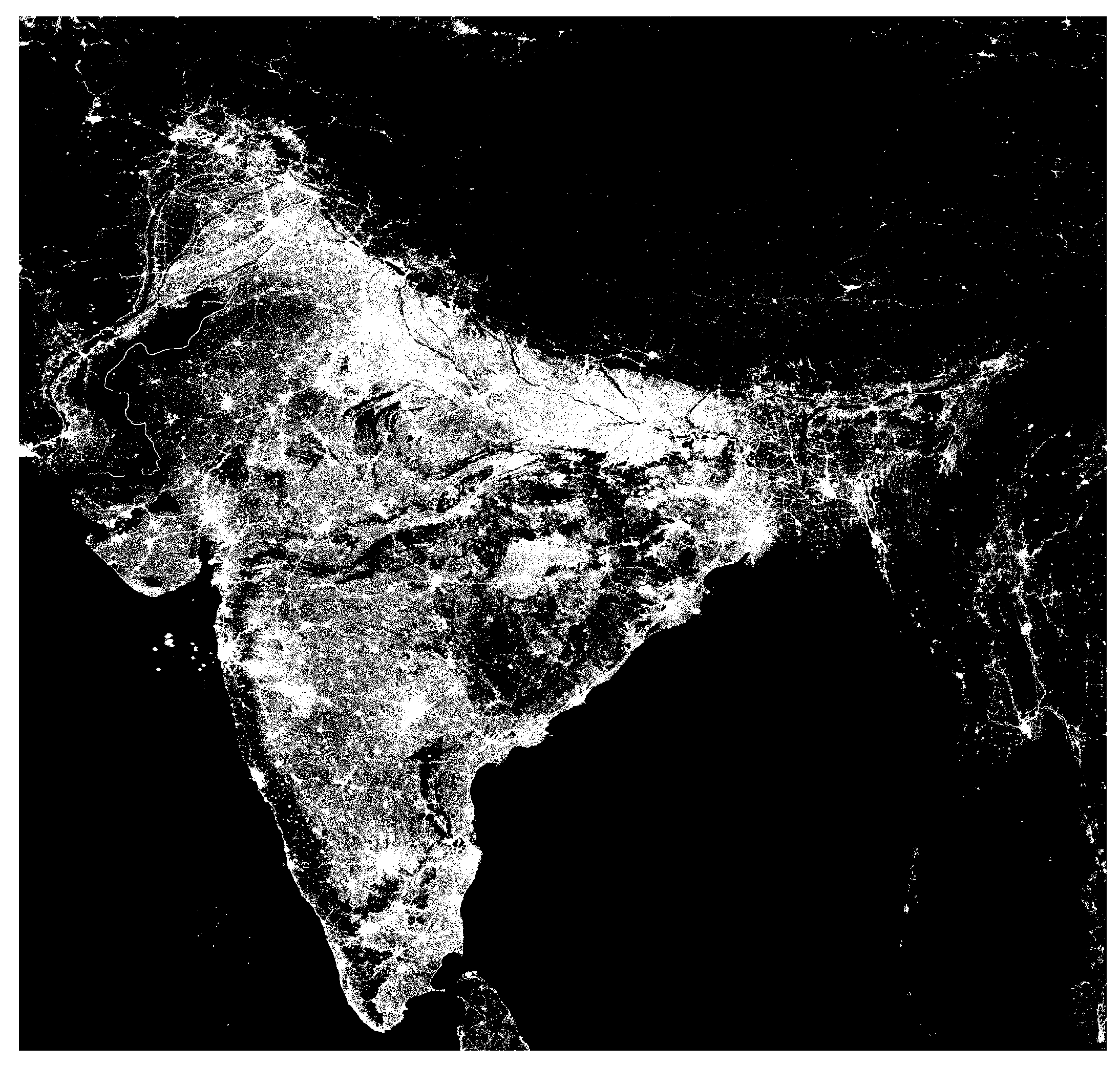
2.1.2. Masking for Lit Areas

Elvidge et al. developed a new annual series of VNL [10]. The new series picked 12 dark locations scattered around the globe, constructing the relationship between the DNB data range and percentage of cloud-free observations. The resultant DNB data range threshold in relation to the percentage of cloud-free observation was then used to determine if the observation from a given location in the annual composite is background noise. The background was filled with zeros. The zeroed out area formed a binary mask. The mask from the 2019 annual VNL was used in this study to mask out non-lit areas.

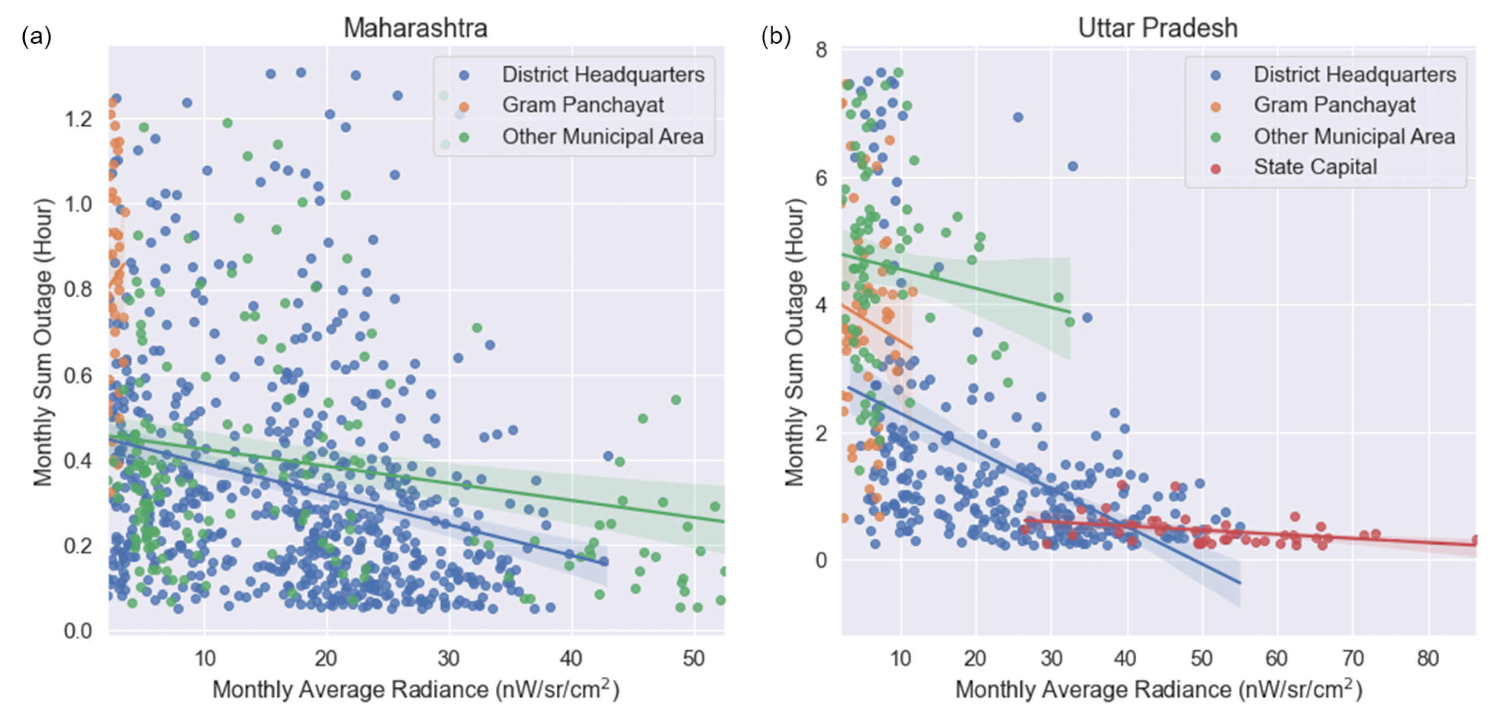
2.1.3. Power Stability Estimates from Survey Data

The India Human Development Survey (IHDS) is a survey that aims to grasp the demographic status of India. The topics of the survey cover aspects such as energy, health, education, culture, etc. The first IHDS (IHDS-1) was carried out in 2004–2005, and IHDS-2 was done in 2011–2012. There was an 85% re-interview rate between the two surveys. IHDS-3 is planned to be released in 2023 [11]. The IHDS compiles the data by states and districts. However, the interviews were not carried out in all the districts of India, so it cannot be said to be nationally representative. Nevertheless, the dataset provides invaluable information describing the socio-economic structure of India in great detail.
For this study, our focus was on the energy section of the IHDS results. Table 1 lists the average percentage of villages with power supply, as well as the average power outage in hours for each state. These numbers are compiled from the IHDS-1 and IHDS-2 datasets.

2.1.4. Power Stability Estimates from Voltage Monitoring

We gathered voltage readings in minutes from the Prayas Energy Group Electricity Supply Monitoring Initiative (ESMI) [12]. Currently, they provide records from 83 sites on their website, and a summary is given in Table 2. Among all states, Maharashtra and Uttar Pradesh have the most locations. The locations of all 81 ESMI voltage monitoring devices are shown in Figure 3. Devices in Uttar Pradesh are mostly installed around Lucknow. Devices in Maharashtra are spread in larger cities like Pune, but none are available in the state capital, Mumbai. The voltage reading precision is +/−4 V, and when reporting 0 voltage, it is regarded as power outage. The installed locations were categorized into four categories, which are the state capital, district headquarters, Gram Panchayat, and other municipal area.

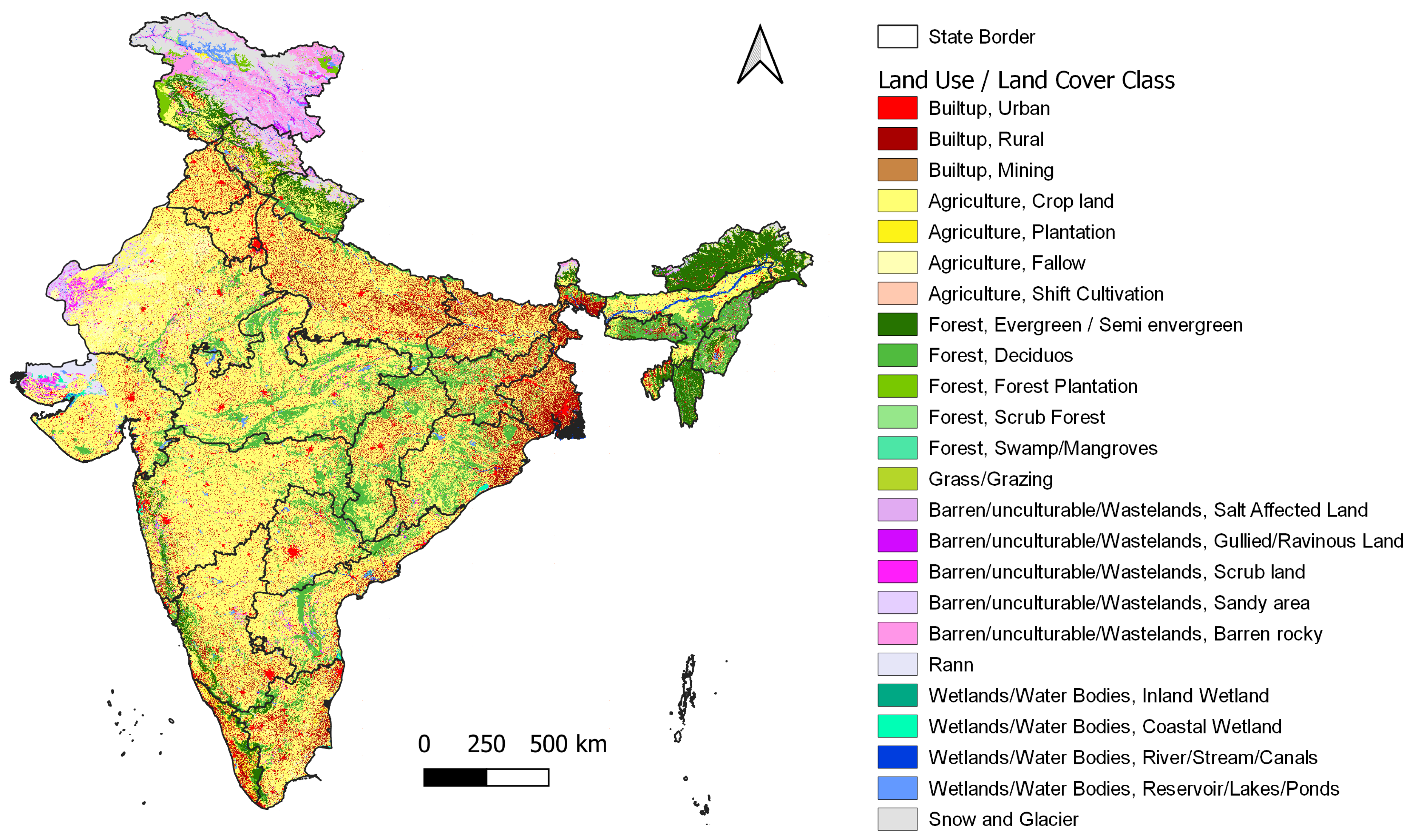
2.2. Land Use/Land Cover

We obtained Land Cover/Land Use (LCLU) data from India’s National Remote Sensing Center (NRSC). The NRSC hosts a 1:50,000 scale LCLU dataset for all states in India via the Bhuvan Web Mapping Service (WMS) [13]. We were able to request the LCLU for each state in 1 degree tiles with dimensions of 2400 × 2400 pixels (1.5 arc second resolution). The retrieved files were in GeoTiff format with RGB bands. The RGB bands were remapped to single band GeoTiff using a palette color table. The color table was customized so that those categories with a higher possibility of light emission had smaller values. The mapping of the original and rearranged LCLU classes and their color palette are shown in Table 3. These single band tiles were then merged to cover the whole study area. Finally, the image was resampled to 15 arc second resolution, taking the minimum value from the sub-pixels. This process ensured that the resampled pixel was represented by the category with the highest interest. The merged 15 arc second LCLU map is shown in Figure 4.

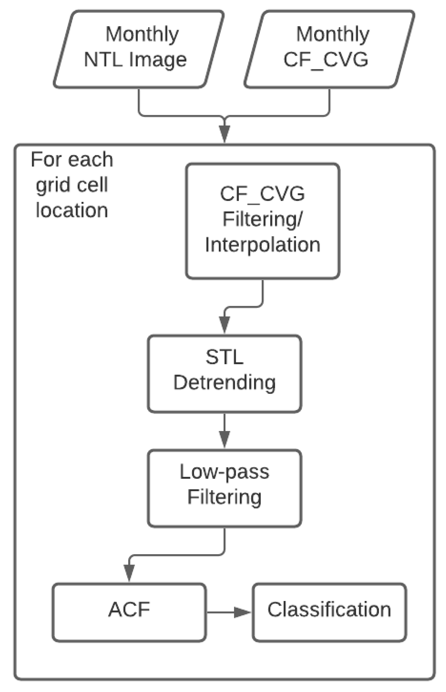
2.3. VNL Image Processing

The main concept of this study is to process the VNL image in the time dimension to extract the temporal information for each grid cell location. Figure 5 shows the overall flowchart of the processing steps as described in the following sections.

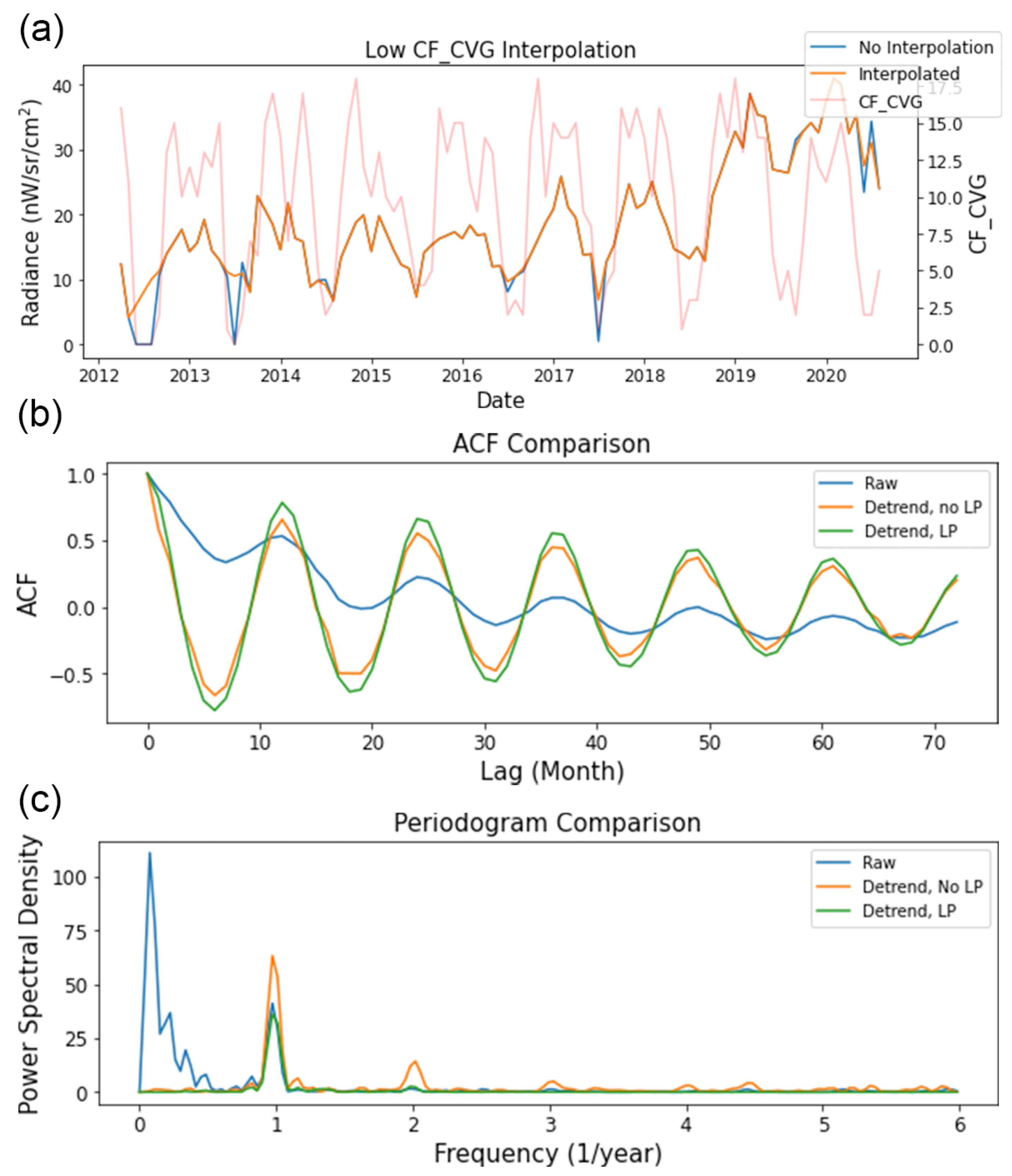
2.3.1. Low Cloud Coverage Treatment

It is difficult for monthly VNL composites to attain 100% coverage over a region every month. The chance of a place being covered by cloud greatly depends on the climate zone and time of year. Therefore, it is important to identify grid cells in the monthly VNL composite that have zero or small cloud-free coverage counts; the resultant average radiance from a small number of observations can be unreliable.
In this study, for each pixel location, the months with zero cloud-free coverage count were removed and replaced by the interpolated value from neighboring months. The months with 1 to 3 cloud-free coverage counts was “blended” by taking the average of its value and the interpolated value from neighboring months. Linear interpolation was used in this process. Figure 6 demonstrates the difference before and after the treatment. Note also that there was a periodical drop of the CF_CVG counts during summer months.

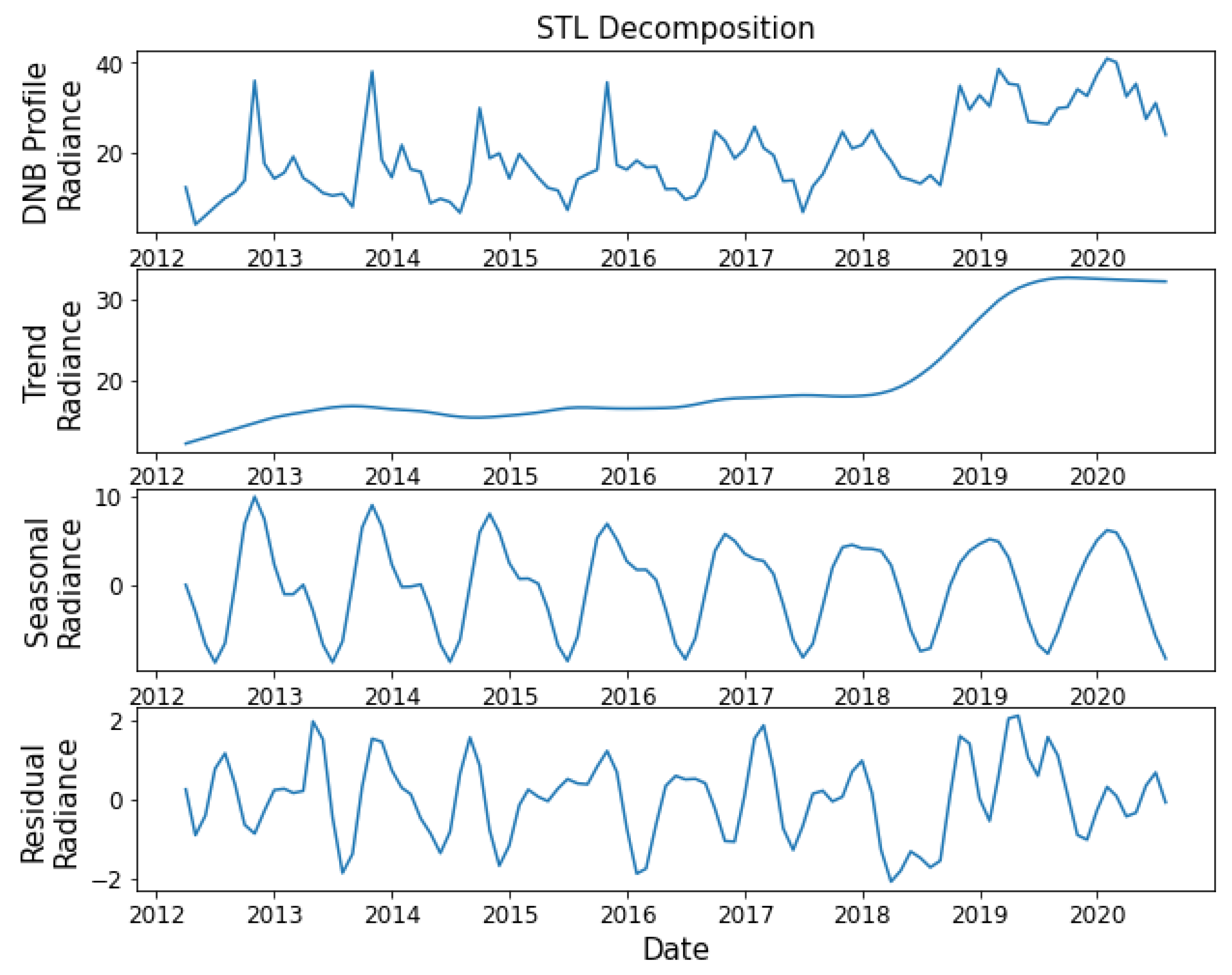
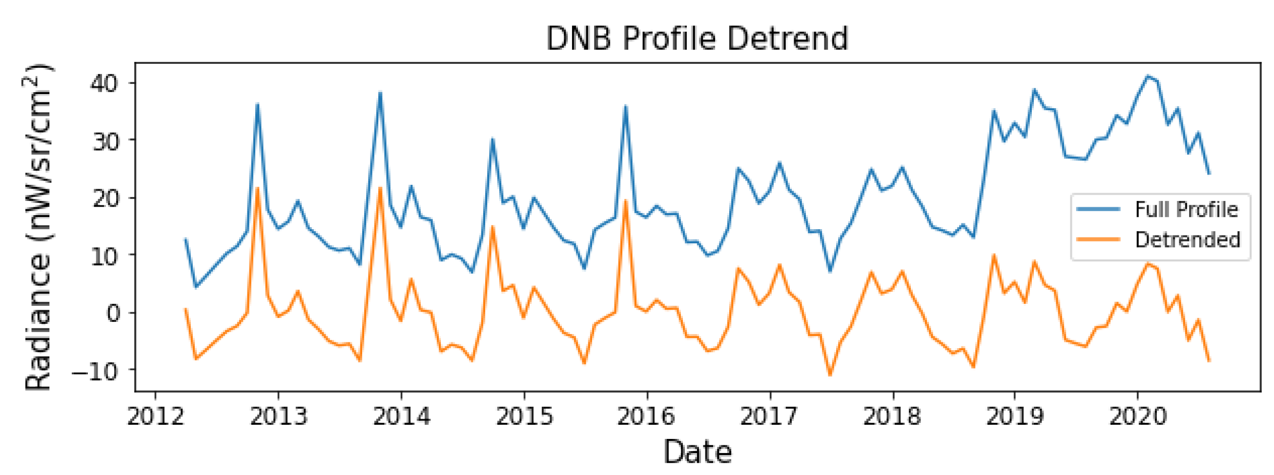
2.3.2. STL Decomposition and Detrending

To study the temporal pattern, it is important to remove the component of long-term trends to reveal finer temporal details. In this study, the trend was extracted from the time series of each grid cell location using Seasonal decomposition of Time series by LOESS (STL) [14]. STL separates a time series into three components: trend, seasonality, and residual. We used the addition model of STL. Thus, the relationship of the input time series and its components can be described as Equation (1). Figure 7 demonstrates the STL result for a VNL time series.
I n p u t = T r e n d + S e a s o n a l i t y + R e s i d u a l
To detrend the VNL profile, we can simply remove the trend in the model as Equation (2). Figure 8 shows the effect before and after detrending the VNL monthly profile.
D e t r e n d e d = I n p u t T r e n d

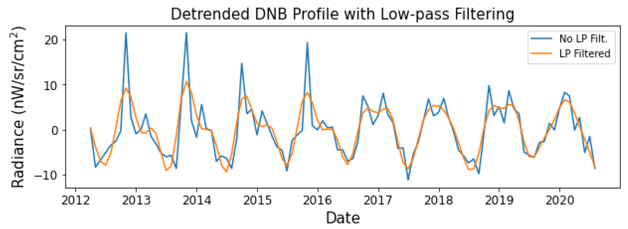
2.3.3. Low-Pass Filtering

Even on cloud-free and low moon nights, the satellite observed light signal emitted from the surface of the Earth still suffers from other elements that are not currently being recognized or corrected during the preparation of the VNL monthly composite; for example, visible lights from biomass burning, light attenuation by atmospheric phenomena, or the viewing angle. These create high frequency noises in the resultant VNL profile. By applying a low-pass filter, it is possible to suppress noises in the high frequency domain and improve the quality of subsequent temporal analysis. In this study, we applied an 8-pole Butterworth filter with the cutoff frequency set at 0.4. By setting the cutoff at 0.4 for a signal with sampling rate of 12/year, the cutoff frequency can be translated to 2.4/year. Upon examining a large number of ACF profiles for grid cell locations in India, it was concluded that the smallest recognizable wavelength was 6 lags, which translates to a frequency of 2/year. Therefore, this cutoff frequency was deemed proper. The profile before and after applying the low-pass filter is shown in Figure 9. The effect of applying the low-pass filter on subsequent temporal analysis will be discussed in the following sections.

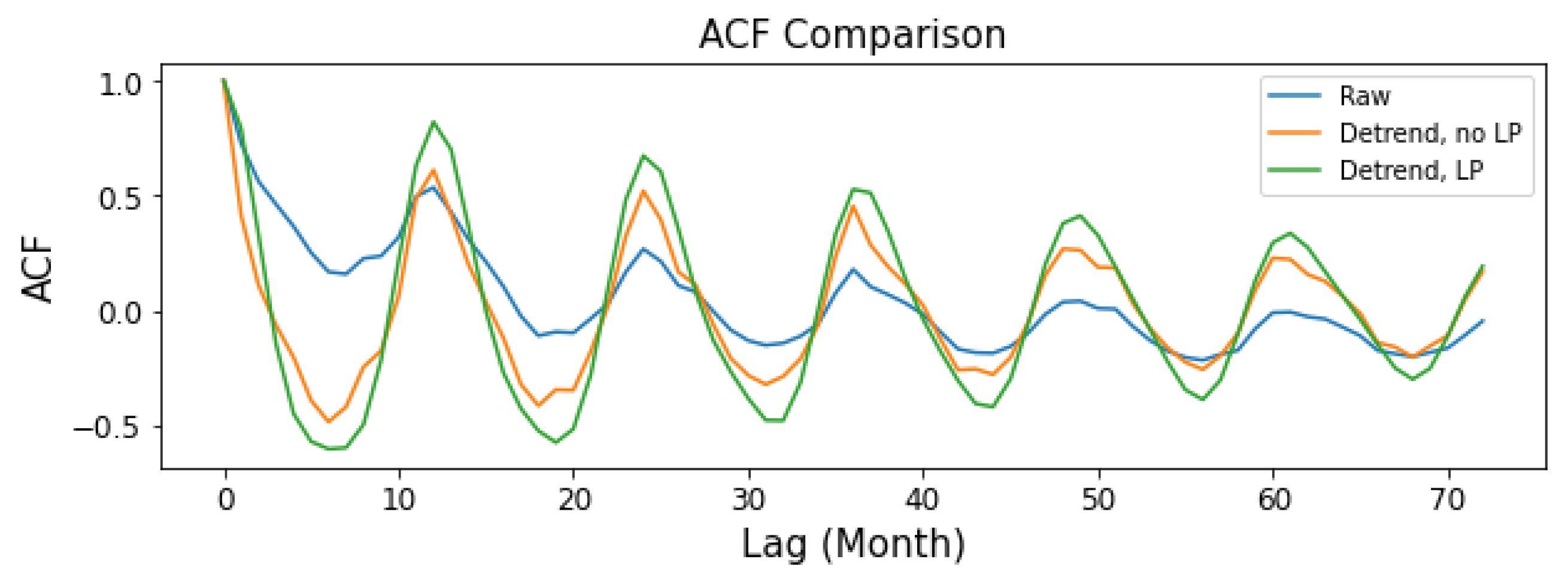
2.3.4. Autocorrelation Function
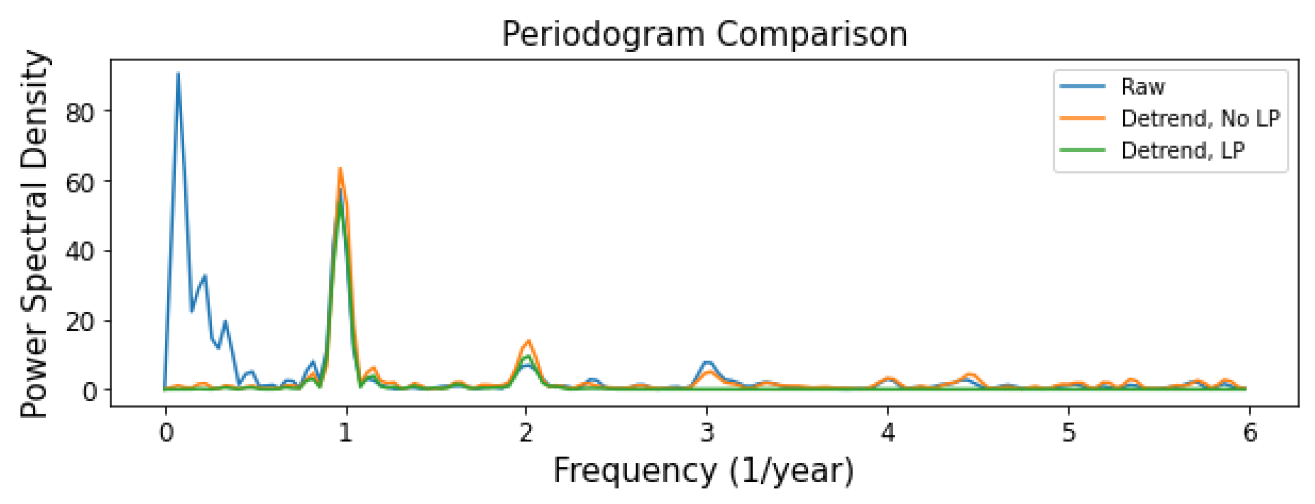
The autocorrelation function (ACF) is one of the very useful tools to describe stationary time series [15]. ACF reveals how the correlation between any two values of the series changes as their separation changes. The distance of separation is called a “lag”. Therefore, ACF at Lag1 will represent the autocorrelation of the series when the position is offset by 1 element. If the first peak in ACF appears at Lag X, this suggests the series has a pattern repeating itself every X elements. The ACF is a robust and quick method to reveal the internal periodicity of the time series data. Figure 10 shows the ACF profile up to 72 lags (months), with series showing the effect on ACF at different preparation stages. It is clear that prior to detrending, the ACF pattern is largely dominated by a smooth descending trend. The finer pattern reveals itself after detrending and is further refined after applying the low-pass filter. The ACF profile shown in Figure 10 has a wavelength ( λ ) of 12 lag, which means there is a pattern in the given VNL monthly profile that repeats every 12 months.

2.3.5. Periodogram

Other than ACF, the periodogram is also a very common tool when it comes to determining the periodic components in a time series. By applying the Fourier transform to the time series and converting the series from the time domain to the frequency domain, we can clearly see how the periodic components stand out as peaks in the frequency domain. As shown in Figure 11, the peak near zero frequency caused by the trend is removed. After applying the low-pass filter, signals with a frequency higher than 2.4/year are removed—a verification of the effectiveness of the low-pass filter. What is left is a primary component at a frequency of 1; and another minor component at a frequency of 2. This indicates that the periodicity of this time series is dominated by patterns repeating once every 12 months. Note that the periodogram has a maximum frequency of half of the sampling rate based on the sampling theorem [15].

2.3.6. Festival Lighting

When working with VNL time series for India, it is natural to think about Diwali and other festivals when people decorate exterior spaces with excess lighting. We compared the result of ACF and the periodogram with and without the Diwali months replaced by interpolated values from neighboring months. We compared the result of the ACF profile and the periodogram with Diwali months removed. The list of months is shown in Table 4. As a result, there was no significant change to ACF and the periodogram, as shown in Figure 12. Figure 12a shows that the peaks in Diwali months were removed and replaced by values interpolated from neighboring months. The resultant ACF shown in Figure 12b indicates that the jitters in the series decreased, and thus the low-pass filter had little effect. As for the periodogram, Figure 12c shows that the primary component was still at a 1/year frequency, with a secondary component at 2/year, diminished after applying the low-pass filter/detrending.
These observations show that heavy festival lighting has little effect on the periodicity analysis. Furthermore, since Diwali is celebrated mainly in northern India, we left Diwali months as is without particular treatment for fairness over our whole study area.

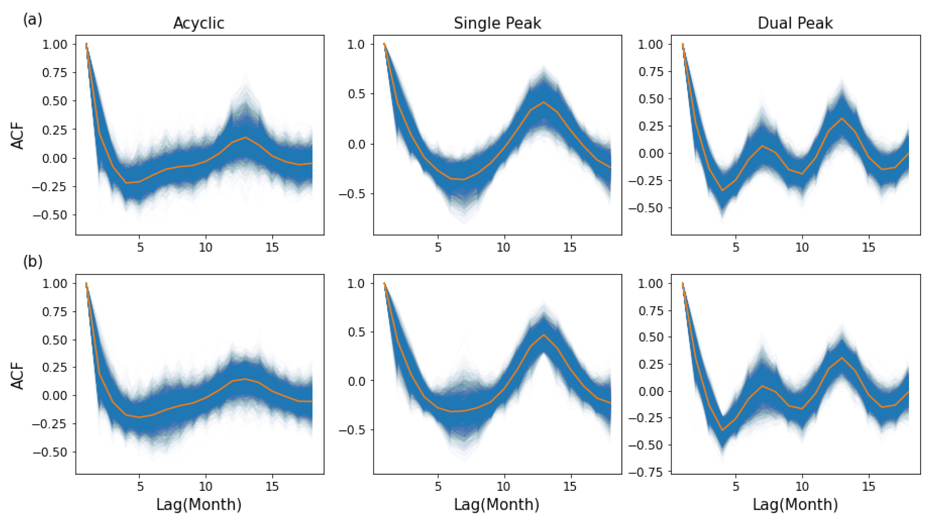
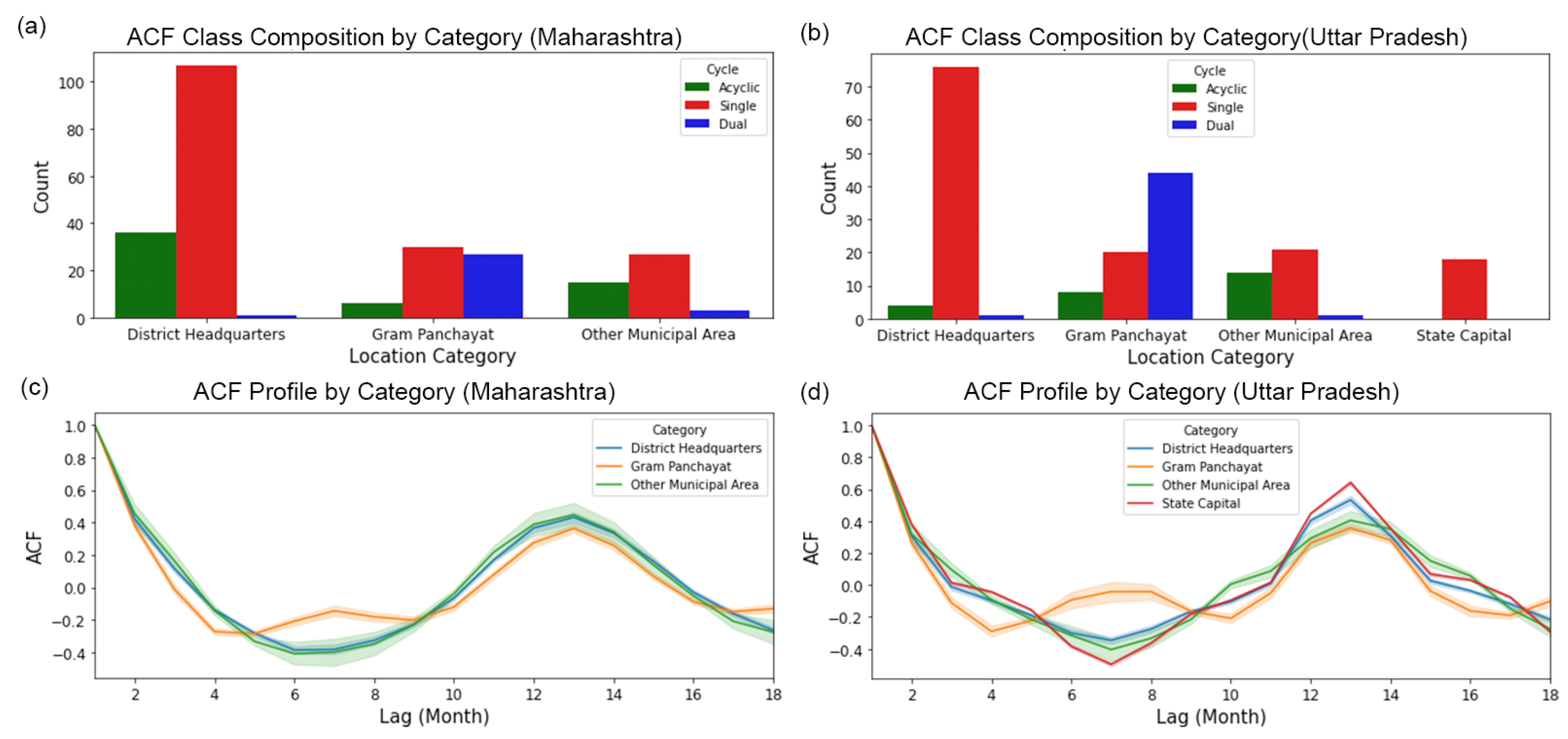
2.4. Classification of Periodic Signature

In this section, we introduce methods used to classify the periodicity of the VNL profile for each pixel location. In this study, we focus on classification based on the ACF profile. Classification with the periodogram is planned in our future studies.
As shown in Figure 12b, ACF is a repetitive signal with a damping amplitude as the lag grows. In our case, the wavelength ( λ ) of the signal is 12 lags. Therefore, it is natural to focus on the first (1+1/2) λ , e.g., the first 18 lags, to study its periodicity. By examining the ACF profile, it was discovered that the annual radiance change can be categorized roughly into three different patterns, i.e., acyclic, single peak, and dual peak. In this study, we did not find any case of more than two prominent peaks within the first 18 lags. The representative patterns of these three classes are shown in Figure 13.
It was assumed that in human settlements, acyclic patterns with moderate to high radiance are a sign of a stable power supply, as they do not show annual variation in brightness. Sufficient power enables higher radiance, while stable supply lessens the seasonal variation of radiance.
Here, we propose two ways to classify the ACF profiles into one of these three classes. The first method employs predetermined rules, and the second is a supervised classification.

2.4.1. Rule Based Classification

An intuitive way to classify the ACF pattern is to count the number of inflection points. The steps can be described in 4 stages as below. The flowchart is shown in Figure 14.
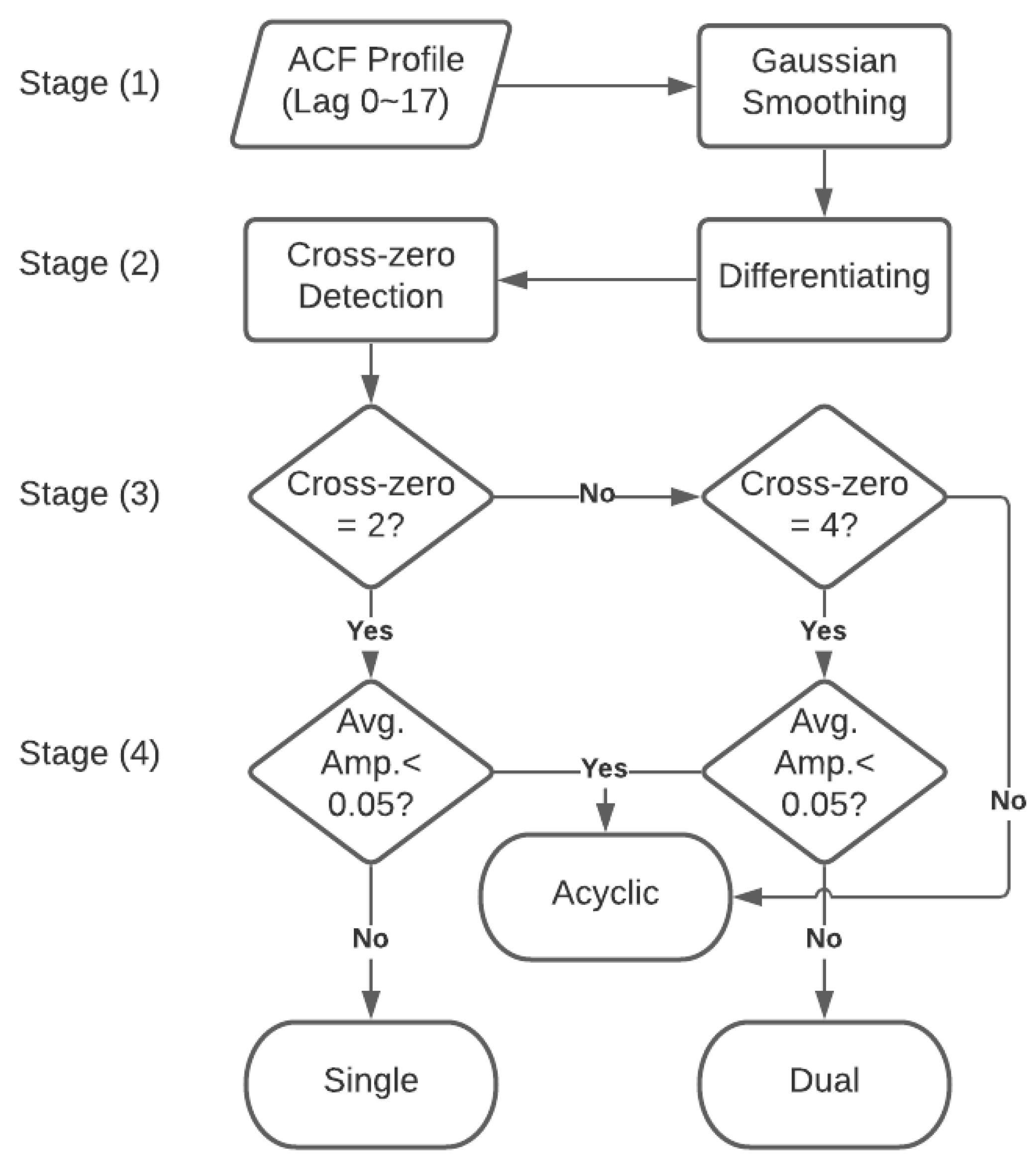
  • Stage (1): Take the ACF from Lag0 to Lag17, and apply the Gaussian filter to the selected section of the ACF profile.
  • Stage (2): Calculate the ACF difference between the lags, then find the zero crossing lags of the difference profile (neglect the first one because it always starts from zero). This stage is essentially taking the second derivative of the ACF profile to find the inflection point.
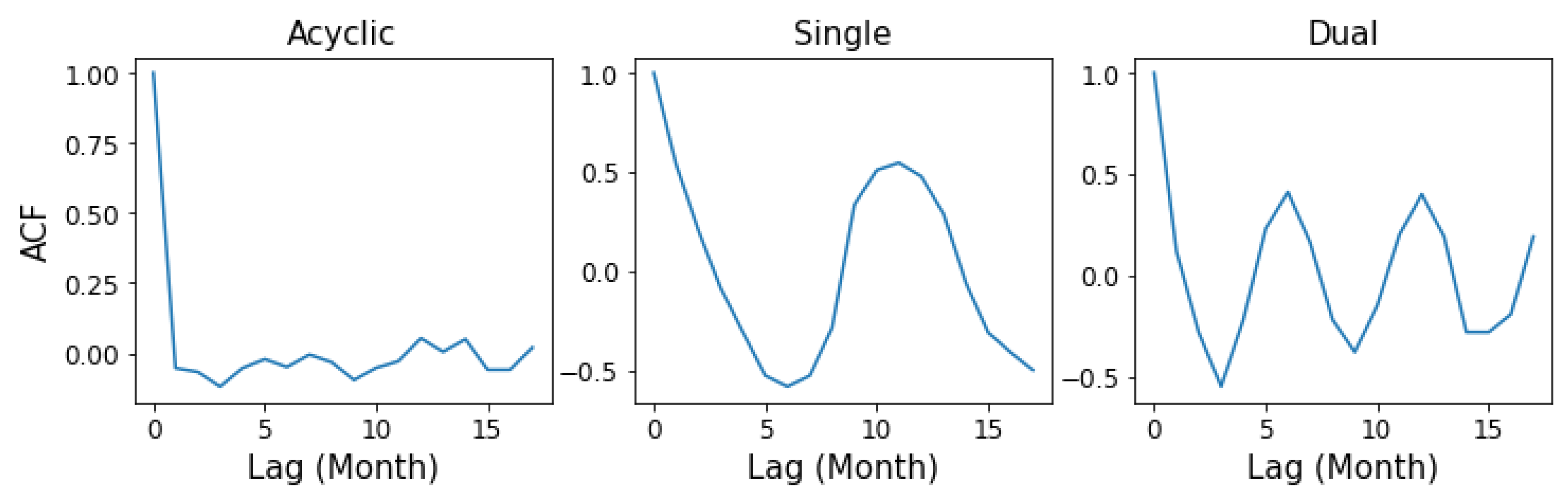
  • Stage (3): Determine the ACF type by counting the number of zero crossing lags. If there are 2 zero crossing lags, then it can be single; if there are 4, it can be dual; otherwise, it is acyclic.
  • Stage (4): Double check the mean amplitude. If it is less then 0.05, then the profile is acyclic. This is to reject false counts of zero crossing caused by small oscillation in the profile.
Stage (4) was designed as a precaution, as it is shown in Figure 15 that only a very small portion of the ACF profiles is processed at this stage.

2.4.2. Supervised Classification

Another way to carry out the classification of ACF cycles is using supervised classification. Here, we demonstrate the procedure with the supervised classification technique in ENVI.
First, a testing site was located in the study area by examining the scatter plot of ACF Lag3 as X and Lag12 as Y. Lag 3is very sensitive to the initial descent of the ACF curve from unity. As shown in Figure 13, the slope of the initial descent is acyclic > dual > single. Lag12 provides a good separation of dual, single, and acyclic. This provides a clear separation between the three arch types of the ACF pattern. A 400 by 400 pixel window found near Lucknow, Uttar Pradesh (location shown in Figure 16f), shows clear clusters of the three features—acyclic, single peak, and dual peak—as shown in Figure 16d. Three classes then were selected based on the scatter plot, covering each signature cluster, as shown in Figure 16e. The corresponding pixels being selected for each group are also color coded as in Figure 16b. Note that not all pixels were selected to be used as training. These pixels were used in training the classifier, which was then applied to the whole study area. For this supervised classification, we used the Mahalanobis classifier to determine the distance of (ACF Lag3, ACF Lag12) for each pixel to the signature group [16,17]. The Mahalanobis distance classifier assigns a given data point to the group with the minimal Mahalanobis distance. In this study, no distance threshold was given in the classification process. The classification result for the sampling area is shown in Figure 16c.

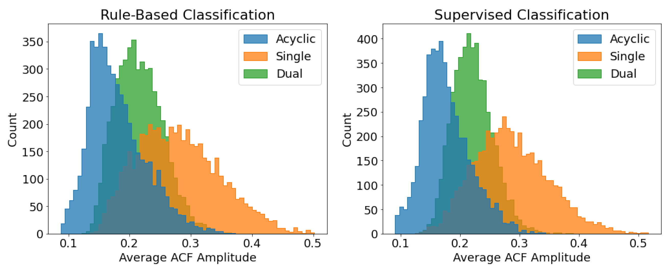
2.4.3. Verifying Classification Results

Since there are no definite ways to acquire the ground truth for cyclic pattern for each grid cell location, to assess the quality of the classified results, the following comparisons were conducted and their results displayed.
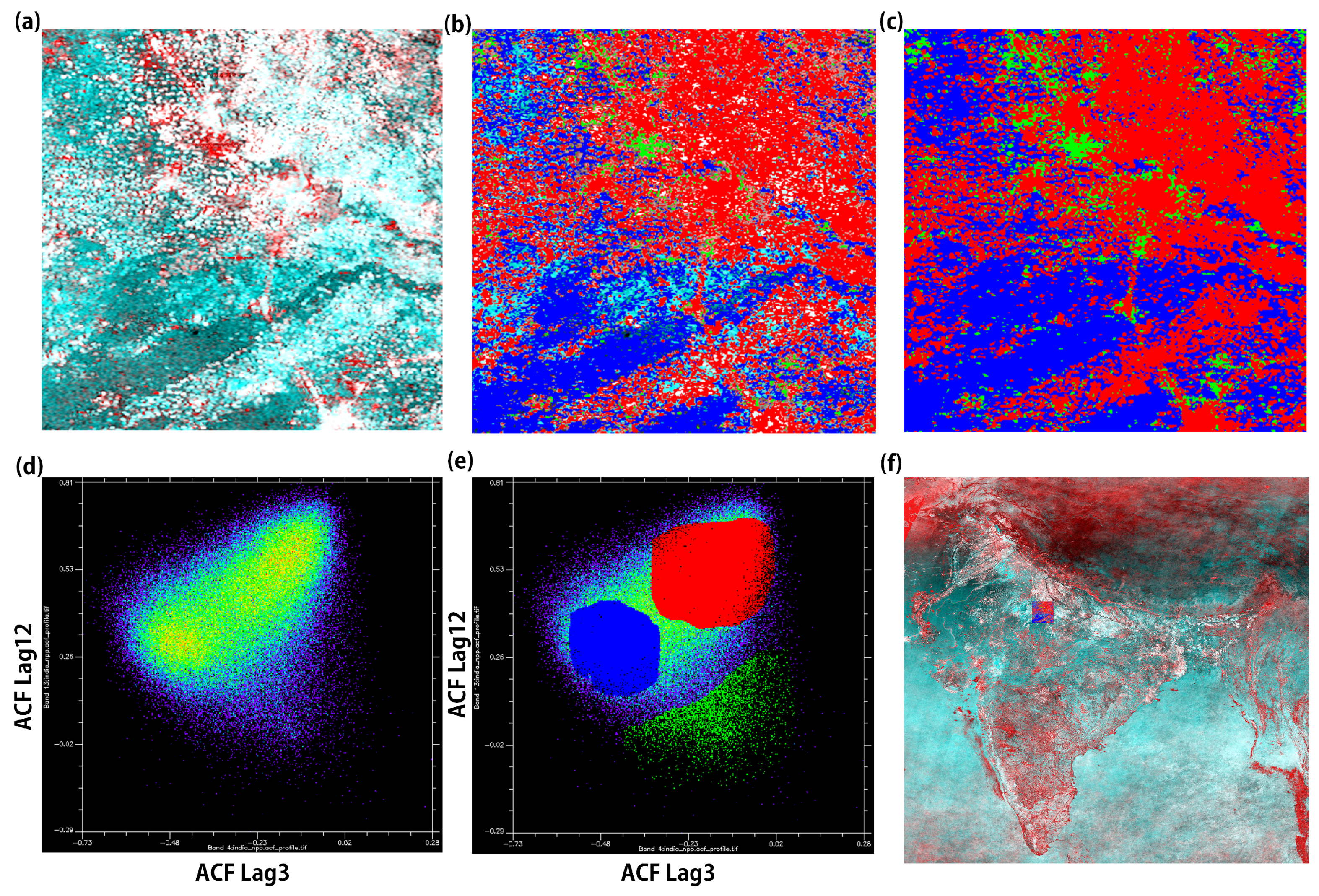
  • Randomly select 5000 samples from each class not masked by the lit area mask and examine if the underlying ACF profile agrees with the assigned class. This is shown in Figure 17.
  • Compare the classified result for each grid cell location from two fundamentally different classification approaches in a comparison matrix. This is shown in Figure 18, and the values are shown in Table 5.
  • Visually compare the classified results from two different classification approaches. This is shown in Figure 15 with a close-up view for an area near Delhi and Figure 19 for the whole study area.
From Figure 17, it is clear that both classification approaches work reasonably well with the average ACF profile from each class matching our typical examples shown in Figure 13 despite small deviations. The resultant average ACF profiles from each category from both approaches highly agree with each other. Next, we take a closer look at the comparison matrix shown in Figure 18 and Table 5. It shows that the classification results from the two approaches have 73.8%, 79.8%, and 61.6% agreement on the acyclic, single peak, and dual peak classes, respectively. Last, we look at Figure 20 and Figure 21, displaying the classification result in the map to visually compare the spatial distribution of the three classes in areas near Delhi and the whole study area covering India. Both figures display a comparable distribution of classes both at the regional and national scale.
We also compared the average ACF amplitude from the same 15,000 samples for both rule based and supervised classification, as shown in Figure 21. It is worth noting that the number of samples having an average ACF amplitude less than 0.05 was very few. In fact, for rule-based classification, almost all cases were classified prior to Stage 4. As designed, Stage 4 was only meant to prevent the acyclic type from being misclassified as other types due to very small oscillations.
The scatter plots of the amplitudes in the periodogram at a frequency of 1/year and 2/year for the three ACF types are shown in Figure 20 with the same 15,000 samples. The amplitude values were normalized by the highest peak in the periodogram. It is clear that the data points from acyclic ACF are randomly scattered because there was no predominant peak tendency. The points from the single peak class show strong clustering towards a high 1/year amplitude and a low2/year amplitude. This indicates a single peak class having a very pronounced frequency component at 1/year. The scatter plot for the dual peak class displays a tendency for a high amplitude at a 2/year frequency, while having a wide spread of the amplitude at a 1/year frequency, indicating the pronounced signature of dual peak ACF with randomly blended single peak components in the frequency domain.

3. Results

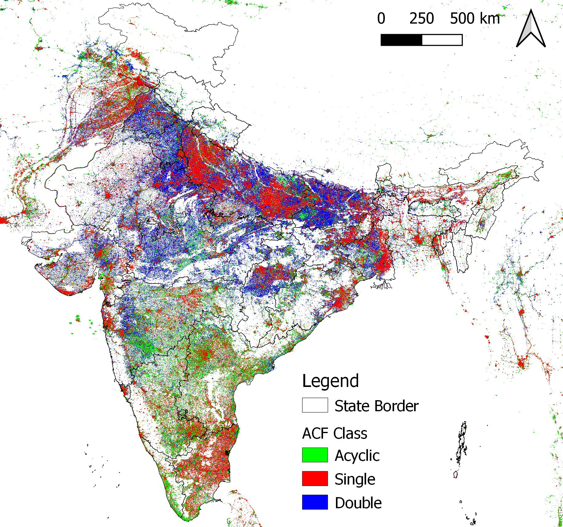
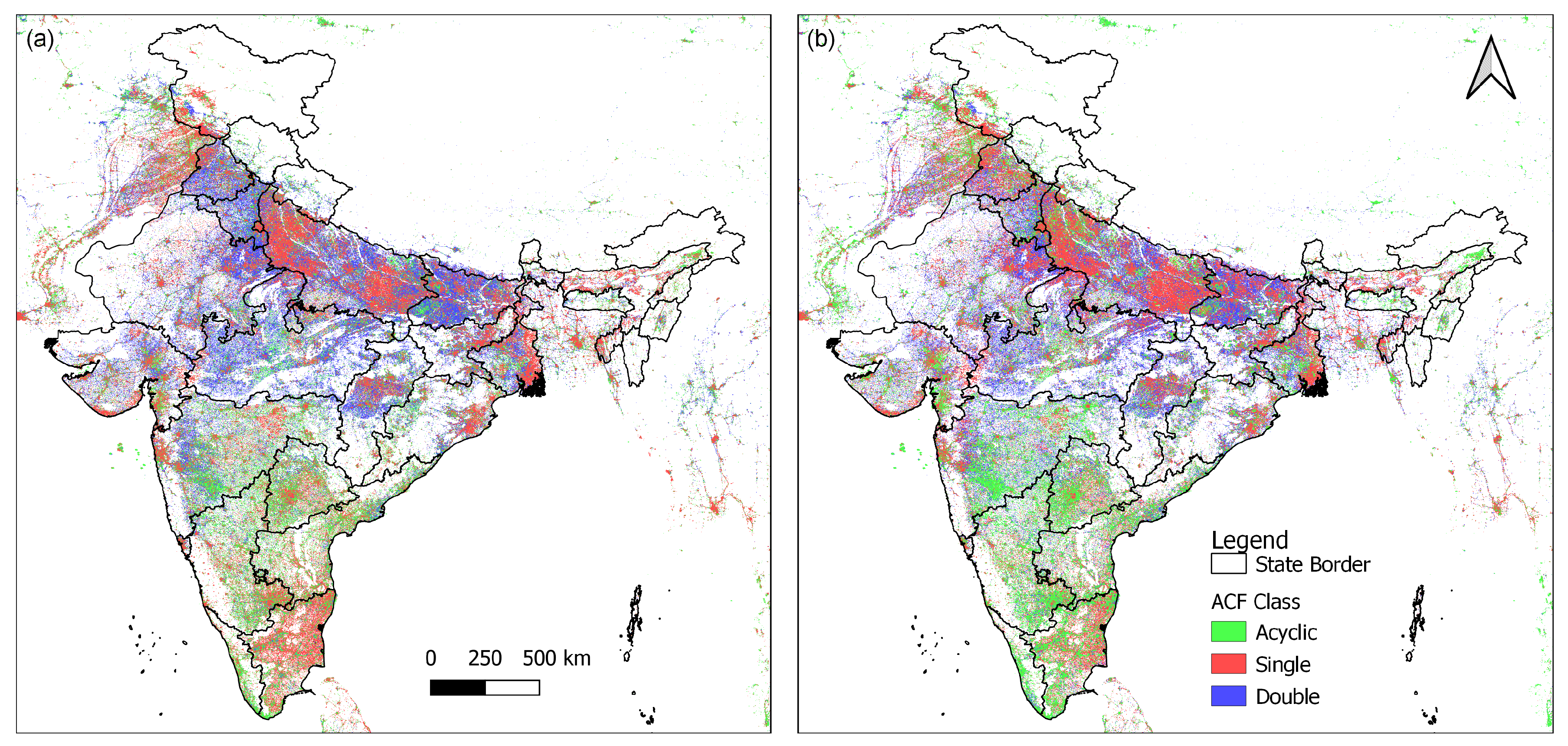
3.1. Spatial Pattern of ACF Class

With the ACF profiles for each pixel location classified, interesting spatial patterns in different regions are revealed.
Industrial light sources are very stable, hence resulting in the acyclic ACF profile. As shown in Figure 22, the offshore oil platforms in the Gulf of Khambhat and refineries near the northern coast of Maharashtra show a strong acyclic ACF pattern.
There is an obvious difference in the ACF class for northern and southern India. As shown in Figure 19, northern India shows more of the dual peak ACF class, while southern India has more of the acyclic class. There is a clear boundary following the border between Madhya Pradesh and Maharashtra. In addition, within the northern states, Uttar Pradesh displays an extensive single peak ACF class on its east and west end, while Tamil Nadu also exhibits an extensive single peak ACF class compared to other southern states.
Figure 15 gives a good close-up view of Delhi and the border between Haryana and Uttar Pradesh. Smaller villages in Haryana show the dual peak ACF class, while those at the west end of Uttar Pradesh show the single peak class. Delhi and the larger cities nearby show the single peak class and are surrounded by a fringe of grid cells with the acyclic class.
Furthermore, in the northwest corner of Panipat, which is a city in Haryana, located to the north of Delhi, there is a cluster of acyclic grid cells, and these grid cells coincide with the Panipat refinery and power plant. The ACF profile for industrial sites is often acyclic, as they are lit with constant brightness most of the time. It is also clear that the NE-2 highway is marked by acyclic pixels. Yamuna River flowing through Delhi and parks are also marked by acyclic grid cells.
Here, we display some more regions of interest at the state level in Figure 23.
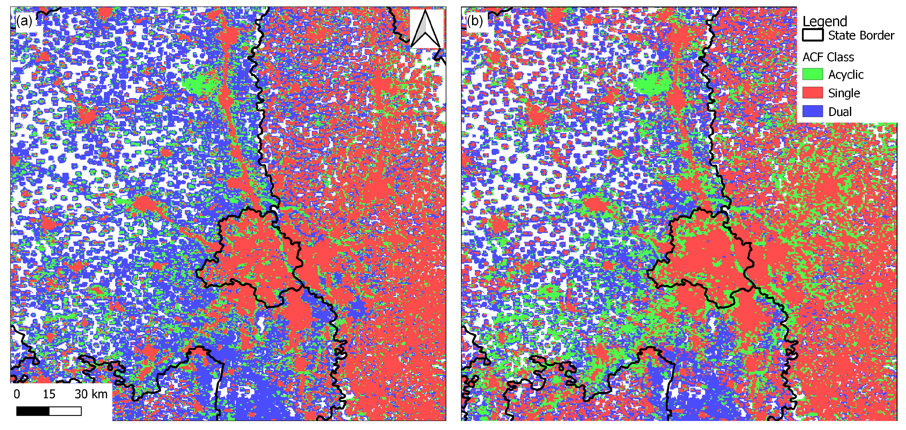
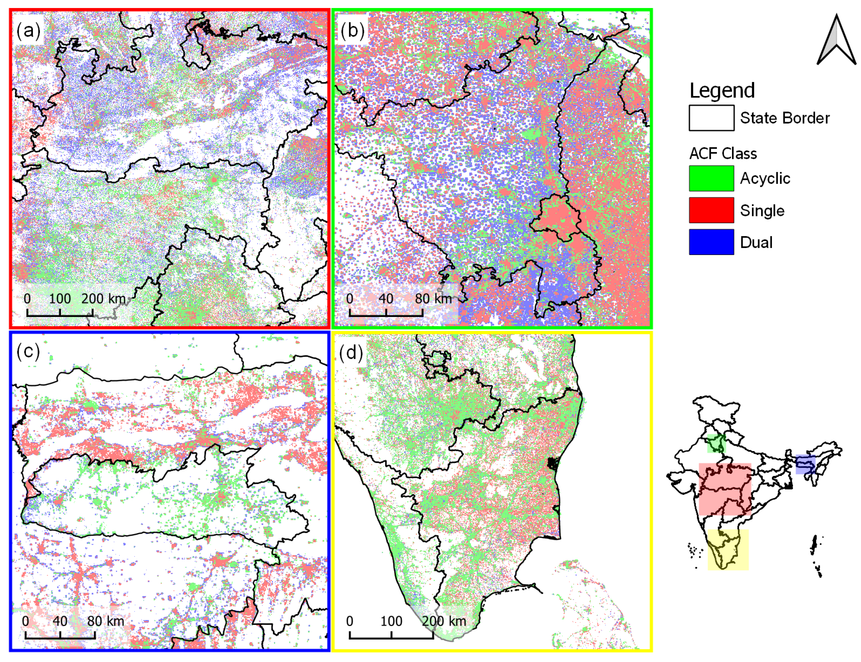
  • Border between Madhya Pradesh and Maharashtra, showing the boundary of ACF class difference between northern and southern India (Figure 23a).
  • Haryana and neighboring states. Displays the ACF class difference between west end of Uttar Pradesh and Haryana (Figure 23b).
  • Meghalaya and neighboring areas. Displays the distinct differences of the ACF class for Meghalaya and Assam on its north and east, as well as Bangladesh to the south (Figure 23c).
  • Tamil Nadu and neighboring states. Tamil Nadu displays a higher fraction of villages with the single peak ACF class than its neighboring southern states (Figure 23d).
There are also regions of interest at the district level, as shown in Figure 24.
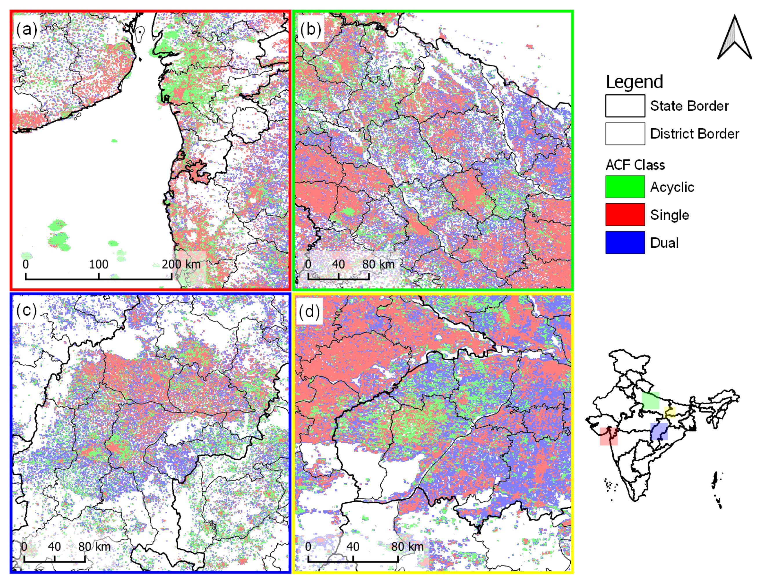
  • Gulf of Khambhat and coast of Maharashtra. Showing gas platforms in the Gulf of Khambhat and refineries near the mouth of Mahi River along the coast of Maharashtra, marked by a cluster of acyclic pixels (Figure 24a).
  • Central Uttar Pradesh shows large areas of smaller villages marked by dual peak pixels. Lucknow and districts to the east and west have more villages with the single peak ACF class; the difference seems to follow the district boundaries (Figure 24b).
  • Chattisgarh. The populated area in Chhattisgarh displays a very different ACF class in the north compared to the south (Figure 24c).
  • Southwestern districts of Bihar. This scene displays a crisp difference of single peak grid cells stopping at the border between Uttar Pradesh and Bihar, while the southwestern districts of Bihar display a large portion of acyclic grid cells compared to their neighbors (Figure 24d).
From these observations, it is clear that urban areas behave differently from rural villages in terms of their ACF class. Next, we attempted to quantify the ACF class between states and between urban/rural areas using the NRSC LCLU data set.

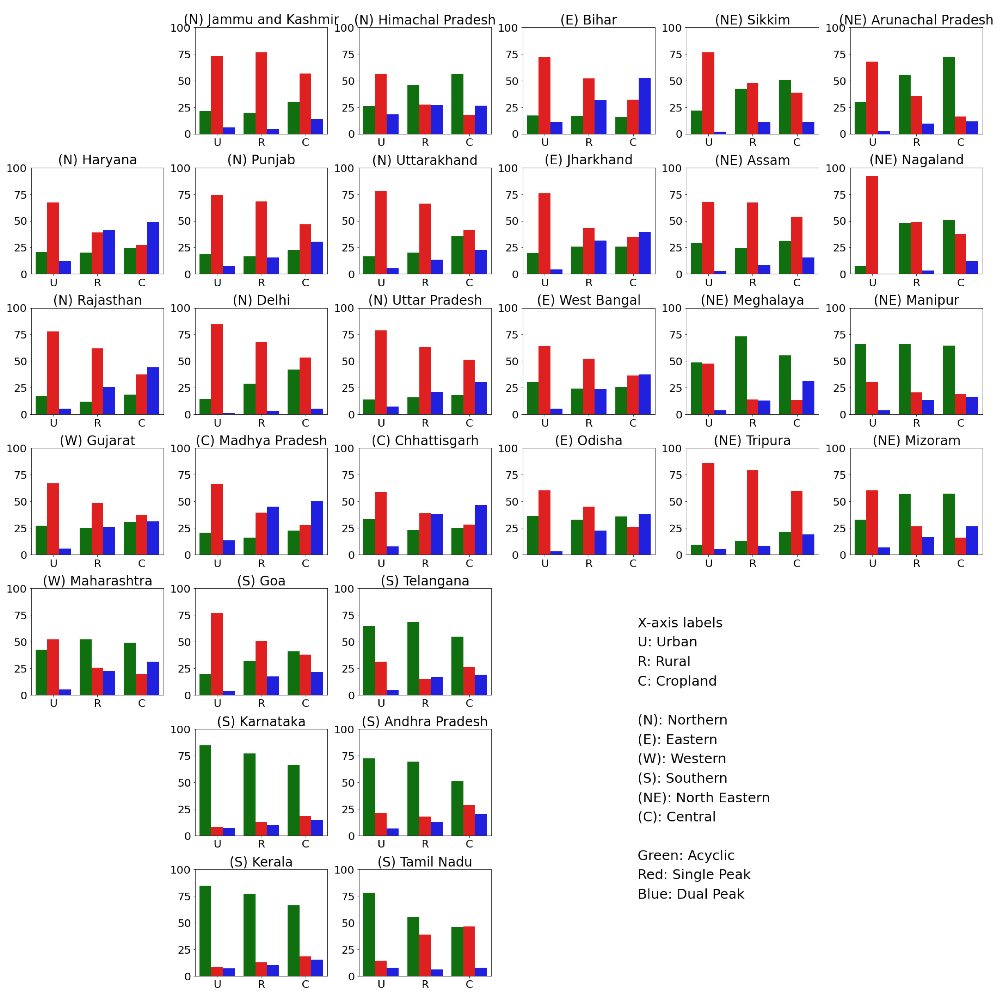
3.2. ACF Class and LCLU Class

To further investigate the regional difference in the ACF class displayed in different states, the NRSC Land Cover/Land Use (LCLU) map was incorporated in this study. Figure 25 shows a grid of state-wise bar plots, arranged by regional groups in relative geographical placement. Only the LCLU classes of urban (built-up, urban), rural (built-up, rural), and cropland (agriculture, crop land) are included, as they are the most dominant LCLU classes in lit areas in India. Note that the NRSC LCLU data set is the only LCLU data that can separate urban and rural populated areas in India. Figure 25 shows some interesting observations that agree with the regional differences in the ACF classification of the NTL monthly profile as described in the previous section.
  • Urban areas in most states are dominated by the single peak class, except Manipur in the northeastern region and the four large states (Karnataka, Kerala, Andhra Pradesh, and Tamil Nadu), which have the ACF class in urban areas dominated by acyclic pattern.
  • Single peaks in the ACF class have a higher appearance in rural areas in northern states, while the four major states in the southern region (Karnataka, Andhra Pradesh, Kerala, Tami Nadu) and some from the northeast (Meghalaya, Manipur, Mazoram, Arunachal Pradesh) show a high proportion of the acyclic pattern.
  • Cropland in northern states has ACF classes all below 50%. Some southern states (Karnataka, Kerala) and NE states (Arunachal Pradesh, Manipur) exhibit a higher proportion of the acyclic pattern in cropland.
  • States exhibiting a higher acyclic pattern in cropland have mountainous terrain. This includes Karnataka, Kerala, and Andhra Pradesh from the southern region, Mizoram, Manipur, Meghalaya, and Arunachal Pradesh from the northeast, and Himachal Pradesh from the northern region.
  • Tamil Nadu exhibits a distinct composition of ACF classes in rural and cropland compared to other larger southern states.
  • Meghalaya exhibits a distinct composition of ACF classes in all three LCLU classes compared to Assam.
  • Madhya Pradesh exhibits a distinct composition of ACF classes in all three LCLU classes compared to Maharashtra.
Given this result of the ACF classes amongst LCLU classes for each state, this implies that the four southern states and Manipur have stable power supply as these states have a high portion of the acyclic pattern in all three LCLU classes. Nevertheless, considering Table 1, these states are not particularly power stable, nor is the coverage great. Compared to Goa and Gujarat, which has less than 1 h of average power outage reported in the IHDS-II survey, they do not show acyclic patterns as the dominant patterns in all three LCLU classes. Therefore, although it is observed that industrial and infrastructure lighting often exhibits the acyclic ACF pattern, there is still room for discussion regarding the relationship of power supply and the ACF pattern when it comes to residential areas.

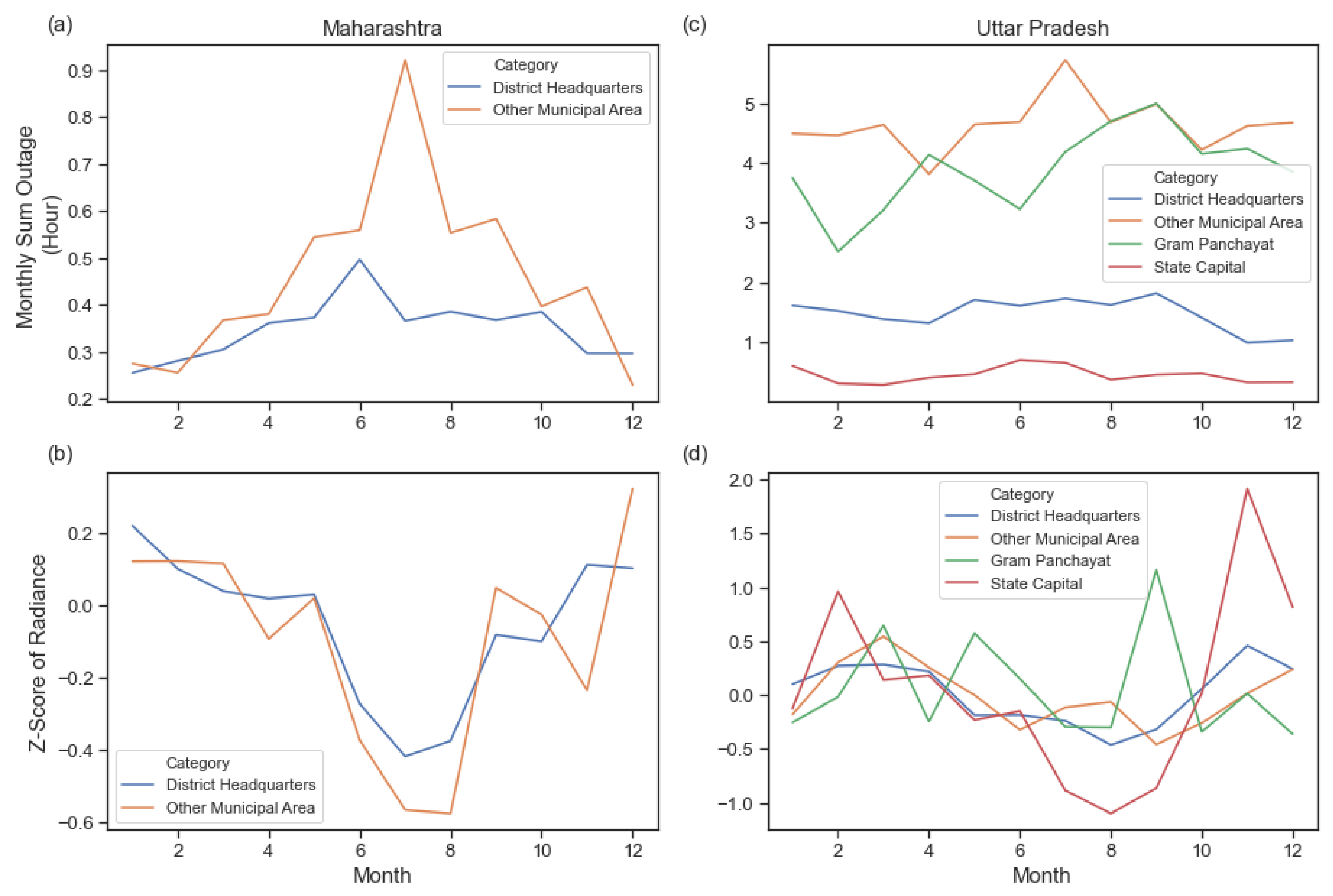
3.3. Power Stability and VNL Brightness

Intuitively, the annual variation of NTL brightness is related to the stability of power supply. It is possible to validate this hypothesis by looking at the Prayas voltage monitoring data and monthly average NTL brightness.
As shown in Figure 26, the monthly radiance tends to be higher when the power outage is less frequent for both Maharastra and Uttar Pradesh. This is most prominent in places categorized as district headquarters and other municipal area. In Figure 27, it is further broken down into the monthly trend. For Maharastra, Figure 27a,b shows that power outage is more likely to happen during summer months, and that is also when the radiance drops. In Uttar Pradesh, as shown in Figure 27c,d, the trend also shows that summer months are dimmer, when the chance of power outage is higher.
This analysis confirms the relationship between power stability and monthly NTL radiance.
We also explored the composition of ACF classes for voltage monitoring locations in Uttar Pradesh and Maharastra. For each voltage meter location, the neighboring pixel locations in a 3 × 3 window were also accounted. The result is shown in Figure 28. For district headquarters, Gram Panchayat, and other municipal area, which are present in collections from both states, their ACF class compositions are comparable. Gram Panchayat in Uttar Pradesh exhibits a higher composition of grid cells classified with dual peak ACF. The voltage meter placard in the state capital is only available in Uttar Pradesh, and it is completely composed of pixels classified with single peak ACF. The composition of ACF classes for each voltage meter location category is clearly reflected in their category-wise ACF profiles.

4. Discussion

As we aimed to characterize the monthly VNL profile for a large area like India with a single index, it is shown that the classification of the ACF profile derived from the monthly VNL profile can be a very descriptive option. Care was taken to prepare the monthly VNL profile for calculating its ACF. Two fundamentally different approaches were proposed to classify ACF into three arch types with good agreement. The resultant classes, namely acyclic, single peak, and dual peak, depicted very different behavior of the monthly VNL profile.
While examining the underlying causes for the variation in the monthly VNL profile with the ACF classes, although it was clear that industrial/infrastructure areas with constant lighting gave acyclic ACF classes, there was room for further investigation mainly because of the spatial discrepancy on how ACF classes were exhibited at every level from national, state, to district.
The NSRC LCLU data set was thus brought in to help provide an additional dimension for how the ACF classes can be quantified. The results gave a clear and definitive view of how ACF classes were different between states and urban/rural areas, confirming the visual observation of the ACF class map.
It is intuitive to link the monthly VNL change and resultant ACF classes to electrical stability. However, the ground truth for electricity stability in India is scarce. In this study, two sources were attempted, i.e., the IHDS and Prayas ESMI. While the IHDS covers most states in India for power outage/penetration estimate, the latest number was for 2011-2012 and did not provide a finer temporal resolution. On the other hand, while Prayas ESMI provided detailed temporal resolution down to a minute, it only covered a handful of locations, mostly in Uttar Pradesh and Maharashtra.
The Prayas ESMI data did confirm that the annual variation of monthly VNL radiance correlated with power stability. That is, months with more unstable power supply might relate to lower monthly VNL radiance. Furthermore, the ACF and its classes also agreed with the observed annual variation of monthly VNL in given voltage monitoring locations.
By comparing what we learned from ACF analysis in conjunction with LCLU to the IHDS numbers, there did not seem to be any consistent connection. While we assumed the acyclic ACF class represents stable lighting behavior, as shown in industrial areas, southern states with most acyclic grid cells in rural areas of Kamataka and Maharashtra do not have optimal power supply in the IHDF-II numbers. On the contrary, some states with a higher proportion of double peak grid cells such as Gujarat are very well powered.
One thing that we do know about the power supply in India is that the nation is still trying its best to meet the demands for electricity from a fast growing economy, while at the same time improving the stability of the power grid. People living in regions with unstable power supply are expected to experience events like load shedding or varying voltage. To cope with such events, it is common to prepare back-up power sources like generators or batteries [2]. One of the major source of nighttime light, i.e., street lighting, has been actively replaced with ones equipped with solar panels [18]. For remote areas, micro grids are also being promoted as an alternative to electricity [2,19].
Other than the power supply, the monthly VNL radiance may also be affected by natural causes such as surface albedo. Artificial lights can be reflected differently by changes in the surface albedo. Note that natural light such as moon light were not discussed because the monthly cloud-free DNB composite only accounts low moon nights. The surface albedo can vary by season. Different crops or rotations, regional climate, or other elements can all contribute to the changes in the surface albedo.
As this is the first work of our investigation into the annual cycling of VNL radiance, we plan to further explore its cause in the following study and pause here for this paper.

5. Conclusions

In this study, we proposed a new approach to analyze monthly VNL radiance profile with ACF. This includes
  • How to prepare the monthly VNL profile for analysis,
  • Defining three arch types of the ACF profile derived from the monthly VNL profile.
  • Proposing two fundamentally different approaches to classify the ACF profile into one of the arch types. The two classification approaches were closely compared to verify whether their results agreed with each other.
The types of ACF for each grid cell location in India were examined, and a clear regional discrepancy was observed on the national and state level. At the national level, northern India exhibited more dual peak ACF, while southern exhibited more single peak ACF. At the state level, different ACF class clusters were formed and sometimes followed the district borders. The popular ACF class also differed depending on the land use class of the grid cell location. Thus, we used the NRSC LCLU data set to further quantify the spatial distribution of ACF classes between states and land use classes; the results confirmed what was learned through visual examination.
It was assumed that the acyclic ACF indicates stable power, while the other two arch types indicate different patterns of power stability. We examined the result both at the small and large scale. At the small scale, the industrial areas and infrastructure with stable lighting showed acyclic ACF. Furthermore, the ESMI data confirmed that the VNL radiance was lower when the chance of power outage was higher, and this corresponded to the resultant ACF class. However, when looking at a larger scale by comparing the state level ACF type composition with the IHDS data, the result was inconclusive. As a result, further investigations into how power stability contributes to the annual cycle of radiance, as well as other possible contributor are required.

Author Contributions

Each of the authors were actively involved in this study. C.E. and M.Z. proposed the idea and prototyped the experiment design. F.H. developed the experiment and analysis and composed the manuscript. T.G. provided extensive local knowledge and advice. J.T. participated in the project conceptualization and editing of the paper. All authors read and agreed to the published version of the manuscript.

Funding

This research was funded in part by the Rockefeller Foundation and NOAA Joint Polar Satellite System (JPSS) proving ground program. The Rockefeller Foundation project name is “Electricity Growth and Use in Developing Economics (E-GUIDE) Center”, Grant Number POW004. The JPSS project is titled “Interpretation of Nighttime Light Change During the COVID-19 Pandemic”, with Steven Miller as the principal investigator.

Data Availability Statement

Classified ACF results are available from https://payneinstitute.mines.edu/eog/.

Acknowledgments

This study relied on the large efforts of NASA and NOAA in generating the long record of nightly VIIRS DNB data and making the data available on an open access basis.

Conflicts of Interest

The authors declare no conflict of interest. The funders had no role in the design of the study; in the collection, analysis, or interpretation of data; in the writing of the manuscript; nor in the decision to publish the results.

References

  1. Load Generation Balance Report. Available online: https://cea.nic.in/l-g-b-r-report/ (accessed on 5 November 2020).
  2. Garg, P. Energy scenario and vision 2020 in India. J. Sustain. Energy Environ. 2012, 3, 7–17. [Google Scholar]
  3. Electricity Demand Pattern Analysis (All India). 2016. Available online: https://posoco.in/reports/electricity-demand-pattern-analysis (accessed on 1 November 2020).
  4. Elvidge, C.D.; Baugh, K.E.; Sutton, P.C.; Bhaduri, B.; Tuttle, B.T.; Ghosh, T.; Ziskin, D.; Erwin, E.H. Who’s in the dark—satellite based estimates of electrification rates. Urban Remote Sens. 2011, 250, 211–224. [Google Scholar] [CrossRef] [Green Version]
  5. Chand, T.K.; Badarinath, K.V.S.; Elvidge, C.D.; Tuttle, B.T. Spatial characterization of electrical power consumption patterns over India using temporal DMSP-OLS night-time satellite data. Int. J. Remote Sens. 2009, 30, 647–661. [Google Scholar] [CrossRef]
  6. Mann, M.L.; Melaas, E.K.; Malik, A. Using VIIRS day/night band to measure electricity supply reliability: Preliminary results from Maharashtra, India. Remote Sens. 2016, 8, 711. [Google Scholar] [CrossRef] [Green Version]
  7. Elvidge, C.D.; Hsu, F.C.; Zhizhin, M.; Ghosh, T.; Taneja, J.; Bazilian, M. Indicators of Electric Power Instability from Satellite Observed Nighttime Lights. Remote Sens. 2020, 12, 3194. [Google Scholar] [CrossRef]
  8. Elvidge, C.D.; Baugh, K.E.; Zhizhin, M.; Hsu, F.C. Why VIIRS data are superior to DMSP for mapping nighttime lights. Proc. Asia-Pac. Adv. Netw. 2013, 35, 62. [Google Scholar] [CrossRef] [Green Version]
  9. VIIRS Nighttime Light. Available online: https://eogdata.mines.edu/products/vnl (accessed on 15 October 2020).
  10. Elvidge, C.D.; Zhizhin, M.; Ghosh, T.; Hsu, F.C.; Taneja, J. Annual time series of global VIIRS nighttime lights derived from monthly averages 2012 to 2019. Remote Sens. 2021, 13, 922. [Google Scholar] [CrossRef]
  11. Indian Humanity Development Survey. Available online: https://ihds.umd.edu/about (accessed on 17 November 2020).
  12. Electricity Supply Monitoring Initiative (ESMI). Available online: https://www.prayaspune.org/peg/resources/electricity-supply-monitoring-initiative-esmi.html (accessed on 1 November 2020).
  13. Bhuvan Thematic Data Dissemination. Available online: https://bhuvan-app1.nrsc.gov.in/thematic/thematic/ (accessed on 15 November 2020).
  14. Robert, C.; William, C.; Irma, T. STL: A seasonal-trend decomposition procedure based on loess. J. Off. Stat. 1990, 6, 3–73. [Google Scholar]
  15. Box, G.E.P.; Jenkins, G.M.; Reinsel, G.C.; Ljung, G.M. Time Series Analysis, 5th ed.; John Wiley & Sons, Inc.: Hoboken, NJ, USA, 2016; ISBN 978-1-118-67502-1. [Google Scholar]
  16. Mahalanobis, A.; Kumar, B.V.; Sims, S.R.F. Distance-classifier correlation filters for multiclass target recognition. Appl. Opt. 1996, 35, 3127–3133. [Google Scholar] [CrossRef] [PubMed]
  17. Mahalanobis Distance. Available online: https://www.l3harrisgeospatial.com/docs/Mahalanobis.html (accessed on 3 November 2020).
  18. Velaga, N.R.; Kumar, A. Techno-economic evaluation of the feasibility of a smart street light system: A case study of rural India. Procedia-Soc. Behav. Sci. 2012, 62, 1220–1224. [Google Scholar] [CrossRef] [Green Version]
  19. Bhoyar, R.R.; Bharatkar, S.S. Renewable energy integration in to microgrid: Powering rural Maharashtra State of India. In Proceedings of the Annual IEEE India Conference (INDICON), India, Mumbai, 13–15 December 2013; pp. 1–6. [Google Scholar] [CrossRef]
Figure 1. Study area map of India, labeling only states.
Remotesensing 13 01199 g001
Figure 2. Nighttime light monthly composite covering India. Showing August 2020 imagery. (a) Cloud-free coverage (CF_CVG) image. (b) Average radiance image.
Remotesensing 13 01199 g002
Figure 3. Map showing the location of ESMI voltage monitor devices.
Remotesensing 13 01199 g003
Figure 4. Land use/land cover map for India.
Remotesensing 13 01199 g004
Figure 5. Flowchart of VNL image processing. SNL, Seasonal decomposition of Time series by LOESS.
Remotesensing 13 01199 g005
Figure 6. Interpolation for low cloud-free coverage (CF_CVG) records.
Remotesensing 13 01199 g006
Figure 7. STL of the VNL monthly profile. DNB, Day/Night Band.
Remotesensing 13 01199 g007
Figure 8. Detrending of the VNL monthly profile using the trend from STL.
Remotesensing 13 01199 g008
Figure 9. Low-pass filtering applied on the detrended VNL monthly profile.
Remotesensing 13 01199 g009
Figure 10. ACF with a comparison at different preparation stages.
Remotesensing 13 01199 g010
Figure 11. Periodogram with the comparison at different preparation stages.
Remotesensing 13 01199 g011
Figure 12. Effect on the VNL profile processing with Diwali months removed and interpolated. (a) VNL profile interpolation with Diwali months removed. Comparison: Figure 6. (b) ACF profile with Diwali months removed. Comparison: Figure 10. (c) Periodogram with Diwali months removed. Comparison: Figure 11.
Remotesensing 13 01199 g012
Figure 13. Representative classes of the ACF profile.
Remotesensing 13 01199 g013
Figure 14. Flowchart of the ACF rule based classification.
Remotesensing 13 01199 g014
Figure 15. ACF classification results’ comparison near Delhi on the map. Lit area mask applied. (a) Rule based classification. (b) Supervised classification.
Remotesensing 13 01199 g015
Figure 16. Classification of ACF into different cycling patterns. (a) Training area showing the RGB composite of ACF Lag3 as red and Lag12 as blue and green. (b) Training samples selected for different categories. The red cluster is the single peak, green acyclic, and blue the double peak. (c) Classification result with Mahalanobis distance classification. (d) Scatter plot of the RGB composite. (e) Samples selected in scatter plot for training. The red cluster is the single peak, green acyclic, and blue the double peak. (f) The location of the training site as shown in the overall study area.
Remotesensing 13 01199 g016
Figure 17. Cycle classification results’ verification with 5000 random samples for each class. (a) Top row showing results from rule based classification. (b) Bottom row showing results from supervised classification.
Remotesensing 13 01199 g017
Figure 18. Comparing classification results from different approaches in a comparison matrix. The height for each bar in the Z axis is normalized by the sum of the pixels in each category from rule based classification.
Remotesensing 13 01199 g018
Figure 19. ACF classification result comparison for two different classification approaches. Lit area mask applied. (a) Rule based classification. (b) Supervised classification.
Remotesensing 13 01199 g019
Figure 20. Comparing the normalized amplitude of the periodogram at a frequency of 1/year and 2/year.
Remotesensing 13 01199 g020
Figure 21. Comparing the average amplitude of the ACF types classified with the rule-based and supervised classification.
Remotesensing 13 01199 g021
Figure 22. Binary background mask from the 2019 annual VIIRS Nighttime Light (VNL) product.
Remotesensing 13 01199 g022
Figure 23. Regions with the supervised ACF classification result of interest. Lit area mask applied. (a) Madhya Pradesh and Maharashtra. (b) Haryana and neighboring states. (c) Meghalaya and Assam. (d) Tamil Nadu and neighboring states.
Remotesensing 13 01199 g023
Figure 24. Regions with the supervised ACF classification results of interest. Lit area mask applied. (a) Region covering the gulf of Khambhat. (b) Central Uttar Pradesh covering Lucknow. (c) Central Chhattisgarh state covering Raipur. (d) Southwestern Bihar.
Remotesensing 13 01199 g024
Figure 25. ACF classes composition of major LCLU classes for every state in India.
Remotesensing 13 01199 g025
Figure 26. Scatter plot showing the relationship of power outage and radiance for (a) Maharashtra and (b) Uttar Pradesh.
Remotesensing 13 01199 g026
Figure 27. The monthly trend of power outage and radiance for Maharashtra and Uttar Pradesh. Upper row: mean monthly total outage hours; lower row: Z-score of monthly NTL radiance. Left column: Maharashtra; right column: Uttar Pradesh.
Remotesensing 13 01199 g027
Figure 28. ACF classes and profiles for each Prayas voltage monitoring location category. (a) ACF class composition by location category in Maharashtra. (b) ACF class composition by location category in Uttar Pradesh. (c) Average ACF profile for each location category in Maharashtra. (d) Average ACF profile for each location category in Uttar Pradesh.
Remotesensing 13 01199 g028
Table 1. Average percentage of villages with power and the average power outage in hours for each state. IHDS, India Human Development Survey.
State
Names
IHDS-II (2011-12)IHDS-I (2004-5)
Average Percentage
of Villages w/ power
Average Power
Outage (hour)
Average Percentage
of Villages w/ power
Average Power
Outage (hour)
Jammu and Kashmir92.915.780.513.5
Himachal Pradesh99.61.598.010.5
Punjab96.04.495.712.8
Uttarakhand91.77.676.410.9
Haryana93.916.490.515.5
Rajasthan80.514.055.617.1
Uttar Pradesh43.616.641.017.2
Bihar37.017.623.521.7
Sikkim90.02.086.77.7
Arunachal100.00.095.85.0
Nagaland97.615.858.213.8
Manipur98.017.584.313.7
Mizoram76.73.776.01.7
Tripura72.36.537.18.9
Meghalaya95.35.380.84.0
Assam58.116.325.119.8
West Bengal67.94.037.88.1
Jharkhand77.113.445.615.0
Orissa60.712.128.49.8
Madhya Pradesh73.415.876.018.0
Gujarat90.20.381.27.6
Maharashtra89.58.077.37.9
Andhra Pradesh91.010.385.18.0
Karnataka89.913.481.812.7
Goa98.30.0100.00.0
Kerala96.324.063.36.0
Tamil Nadu92.612.280.64.0
National Average83.310.269.010.8
Table 2. Breakdown of voltage monitoring devices available from the Prayas Electricity Supply Monitoring Initiative (ESMI) website.
State
Name
CategoryCount
State
Capital
District
Headquarters
Gram
Panchayat
Other
Municipal Area
Karnataka22217
Maharashtra0167528
Bihar00101
Uttar Pradesh298423
Tamil Nadu10012
West Bengal10001
Andhra Pradesh/Telangana30003
Madhya Pradesh12003
Assam20002
Telangana10001
Goa01203
Odisha20002
Andhra Pradesh00011
Gujarat01001
Chandigarh (UT)10001
Chhattisgarh10001
Punjab01001
Total1732201281
Table 3. LCLU class definition and palette.
Rearranged
Order
Original
Order
Color BandClass Name
RGB
1125500Built-up, Urban
2216800Built-up, Rural
15320013368Built-up, Mining
34255255115Agriculture, Crop land
4525324323Agriculture, Plantation
76255255181Agriculture, Fallow
87255201176Agriculture, Current Shifting Cultivation
58381150Forest, Evergreen/Semi-Evergreen
698018762Forest, Deciduous
11101212000Forest, Forest Plantation
1211150231138Forest, Scrub Forest
131276230166Forest, Swamp/Mangroves
141318121441Grass/Grazing
161425171242Barren/Unculturable/Wastelands, Salt Affected Land
171521010255Barren/Unculturable/Wastelands, Gullied/Ravinous Land
181625530250Barren/Unculturable/Wastelands, Scrub land
1917229207255Barren/Unculturable/Wastelands, Sandy area
2018255150232Barren/Unculturable/Wastelands, Barren rocky
2119230230248Rann
22200168132Wetlands/Water Bodies, Inland Wetland
23210255181Wetland/Water Bodies, Coastal Wetland
922061222Wetland/Water Bodies, River/Stream/Canals
102399253255Wetlands/Water Bodies, Reservoir/Lands/Ponds
2424225255225Snow and Glacier
Table 4. Diwali months removed for test.
YearMonth
201211
201311
201410
201511
201610
201611
201710
201811
201910
202011
Table 5. Comparing the classification result from different approaches in a comparison matrix with values normalized to the sum of the pixels in each category from rule based classification.
Rule Based
AcyclicSingleDual
SupervisedAcyclic73.8%13.4%30.9%
Single12.9%79.8%7.5%
Dual13.2%6.8%61.6%
Sum100%100%100%
Publisher’s Note: MDPI stays neutral with regard to jurisdictional claims in published maps and institutional affiliations.

