In this section, the proposed method is presented in detail. We first overview the architecture of the proposed BARNet briefly. Then, the proposed gated-attention refined fusion unit, denser atrous spatial pyramid pooling module, boundary-aware loss and training loss are elaborated.
3.1. Model Overview
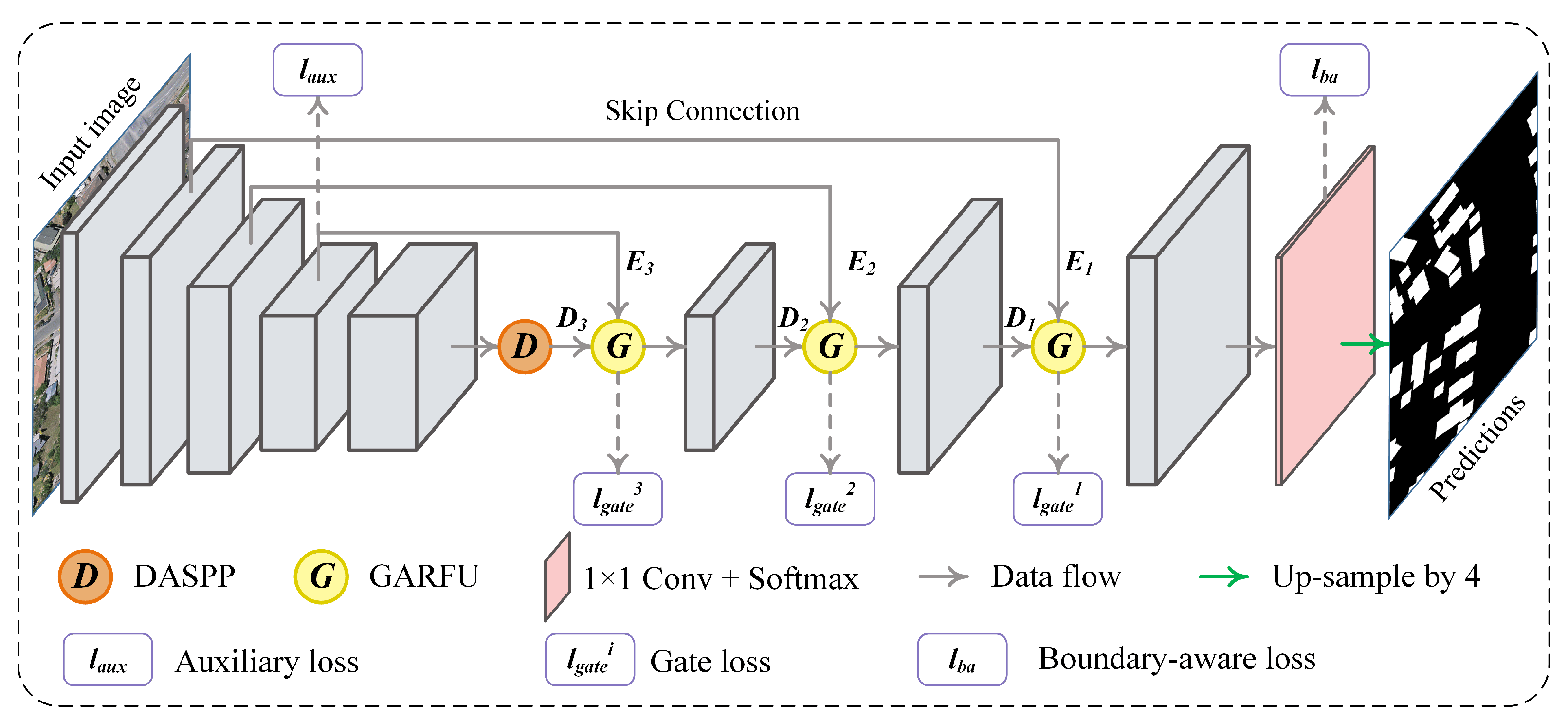
The BARNet takes VHR aerial images as the input and performs pixel-level building extraction in an end-to-end manner. As illustrated in
Figure 2, the BARNet is a standard encoder-decoder structure composed of three parts: encoder, context aggregation module and decoder. ResNet-101 [
16] is adopted as the backbone network to encode the basic features of buildings. The fully-connected layer and the last global average pool layer in ResNet-101 are removed. To retain more details in the final feature map, for the last stage of ResNet-101, all
convolutions are modified with dilated convolutions with dilated rates of
, and the stride in the down-sampling module is set to 1. After the encoder, DASPP is appended to capture the dense global context semantics. Before harvesting the low-level features into the decoder, each low-level feature map from the encoder is reduced to 256 channels with a
convolution layer followed by Batch Normalization (BN) and ReLU layers, for less computational cost. The reduced low-level feature map and the corresponding high-level feature map from the decoder are fused in the GARFU. Then, the fused features are fed into the decoder block to restore the details. Each decoder block in the BARNet is equipped with two cascaded Conv-BN-ReLU blocks, the same as U-Net and DeepLab-v3+. At the end of the BARNet, a
convolution layer and a softmax layer are applied to output the final predictions. To get the same size as the original input, the final predictions are further up-sampled by 4 times using bilinear interpolation.
3.2. Gated-Attention Refined Fusion Unit
The significant highlight of U-Net and FPN is integrating the cross-level features via simple concatenation and addition operations. Given a low-level feature map
and a high-level feature map
, in which
i,
C,
H and
W denote the level order, number of channels and height and width of the feature map, respectively, the two basic fusion strategies can be formulated as:
where
denotes the concatenation operation,
means the up-sampling operation and
represents the fused feature map. It can be evidently observed from the above two equations that all feature maps are fused directly without considering the contribution of each feature. As described earlier in
Section 2.2, different level features are complementary, which is beneficial for building extraction. However, to the best of our knowledge, the informative features in a feature map are mixed with massive redundant information [
42]. As a result, the cross-level features should be re-calibrated before combining them for the best exploitation of the beneficial features. To achieve this goal, we developed the GARFU. As presented in
Figure 2, the GARFU is embedded at each short-cut, which only incurs a small extra computational cost.
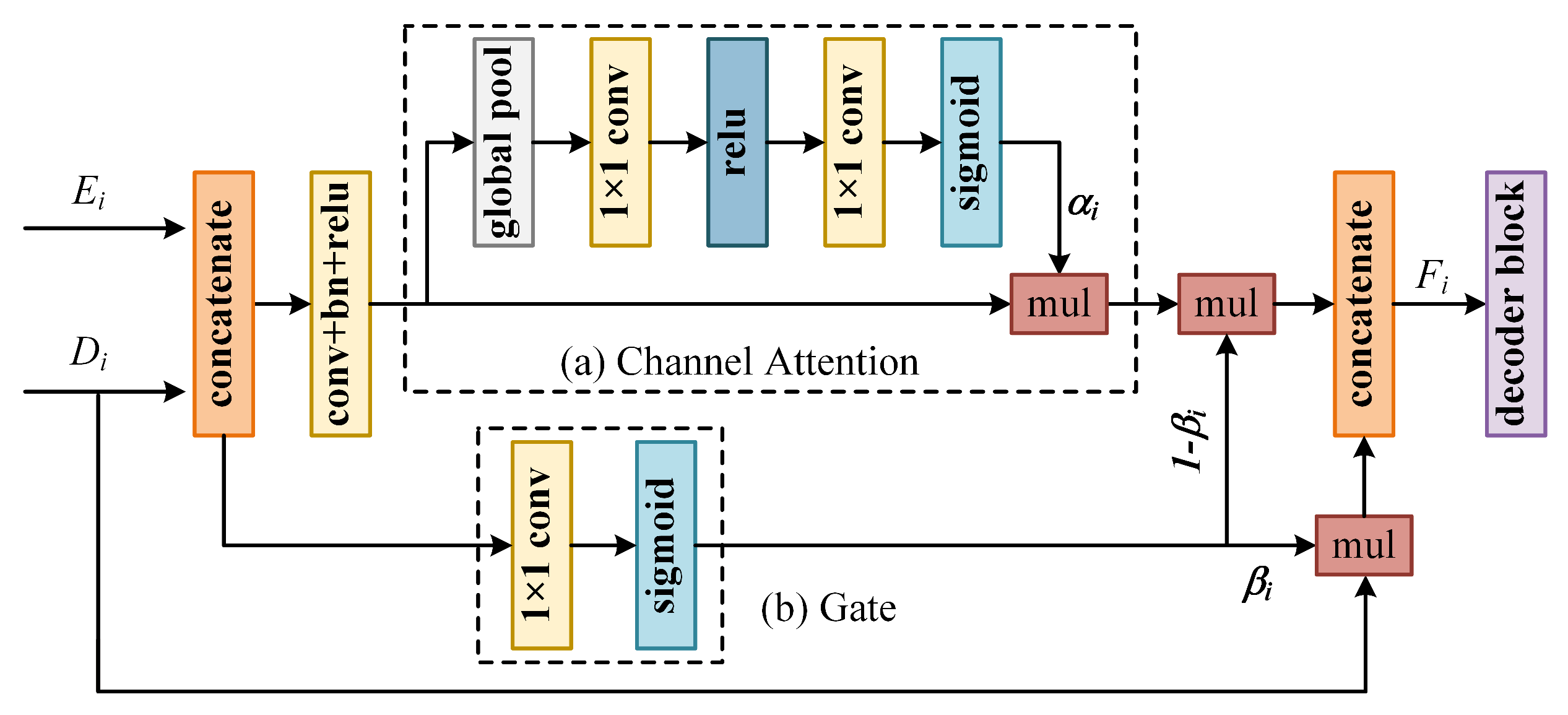
The GARFU consists of two major components: the channel-attention module and the spatial gate module. As displayed in
Figure 3, the low-level feature map
is first re-calibrated by a channel-wise attention vector
. Then,
and
are re-calibrated by multiplication of a gated map
and
, respectively, in which
. The mechanism of the GARFU can be defined as:
where
represents the multiplication in the channel axis and
represents the multiplication in the spatial dimension.
(1) Channel attention: The latest works demonstrated the effectiveness of modelling the contribution of each channel using the channel attention mechanism [
1,
43]. Therefore, we adopt the channel attention module reported in SENet [
43] to exploit channel-wise useful features in the low-level feature map, because the low-level features usually carry more noise. The attention vector
is generated based on the concatenated result of
and
. Before concatenating them,
is first up-sampled with bilinear interpolation to make
have the same spatial shape as
. Then, the concatenated features are passed through a
convolution layer for less parameters. Let
, where
c are the concatenated features and
is the channel-wise global average pooling operation. The attention vector
is obtained by:
in which
and
are two linear transformations,
denotes the ReLU activation function and
is the sigmoid activation.
is multiplied by
to enable the network to learn the salient channels that contribute to distinguishing buildings.
(2) Gate: Many studies [
26,
27,
30] suggested that introducing the low-level information can improve the accuracy of predictions on the boundary and details, whereas lacking global semantics may lead to confusions in other regions due to a limited local receptive field size. On the other hand, there exists a semantic gap for low- and high-level features, that is not all features benefit building extraction. With this motivation, we adopt the gate mechanism to generate a gate map
, which serves as a guide to enhance the informative regions and suppress the useless regions both in low- and high-level features. Gates are widely used in deep neural networks to control the information propagation [
44]. For example, the gated recurrent unit in the LSTM network is a typical gate [
45]. In this work, the gate
is generated by:
where
W is a linear transform parameterized with
,
denotes sigmoid activation for normalizing the value into
and
is a trainable scale factor to prevent the minima occurring during the initial training. The gate map is learned under the supervision of the ground-truth during training, and the pixel value in it measures the degree of importance for each pixel. The feature at position
would be highlighted when the value of
is large, and vice versa. In this manner, the useless information is suppressed, and only useful features can be harvested to the following decoder block, thus obtaining better cross-level feature fusion. Different from the self-attention mechanism, the gate is learned with the explicit supervision of the ground-truth.
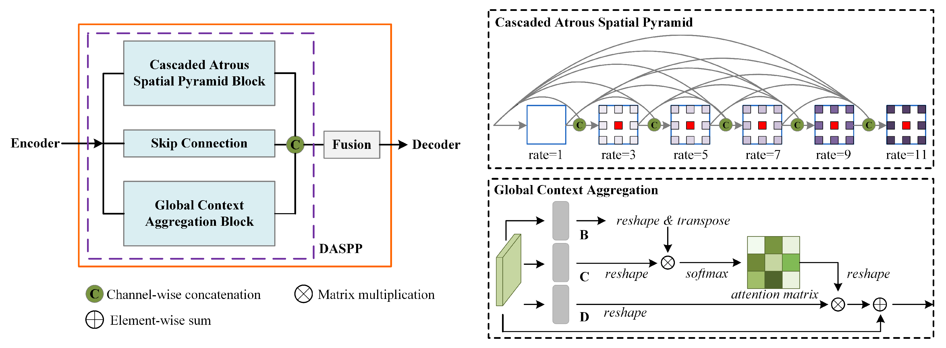
3.3. Denser Atrous Spatial Pyramid Pooling
As is well known, building scale variance frequently occurs in complex urban scenes, resulting in non-unified extraction scales. Thus, an ideal context modelling unit should capture the dense multi-scale features as much as possible. To achieve this goal, a new ASPP module is developed. As it is inspired by ASPP and the main idea is to capture the denser image pyramid feature, we name it denser atrous spatial pyramid pooling. As illustrated in
Figure 4, the DASPP module consists of a skip connection, a Cascaded Atrous Spatial Pyramid Block (CASPB) and a global context aggregation block. The skip pathway is only composed of a simple
convolution layer, aiming at reusing the high-level features and accelerating network convergence [
16]. In CASPB, we cascade the hybrid multiple dilated
depthwise separable convolution [
46] layers with different dilation rates and connect them with dense connections. Here, the depthwise separable convolution is utilized for reducing the parameters of DASPP, and the negative effect is almost negligible. The CASPB can be formulated as
, where
represents the dilatation rate of the
ith layer
L,
means the convolution operation and
denotes the concatenation operation. In this study,
. Compared to ASPP, this change brings us two main benefits: a denser feature pyramid and a larger receptive field. The sequence of the receptive field size in the original ASPP is 13, 25 and 37, respectively, when the output stride of the encoder is 16. However, the max receptive field of each layer in the CASPB is 3, 8, 19, 36, 55 and 78, which is denser and larger than ASPP. This means the CASPB is more robust with the building scale variations. In addition, the position-attention module of DANet [
36] is also introduced to replace the image pooling branch in ASPP to generate denser pixel-wise global context representation. Unlike the global average pooling used in PPM and ASPP, the self-attention can a generate global representation and capture the long-range dependence between each pixel. As presented in
Figure 4, the position-attention module re-weights each pixel according to the degree of correlation between any pixels.
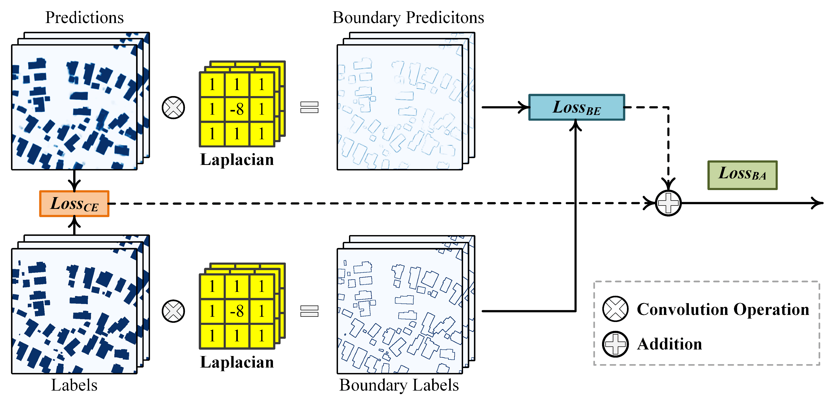
3.4. Boundary-Aware Loss
Although the re-calibrated low-level features contribute to refining the segmentation results [
30], this is still not sufficient enough to locate accurate building boundaries. As mentioned earlier, the commonly used per-pixel cross-entropy loss treats each pixel equally. In fact, depicting boundaries is more challenging than locating semantic bodies because of the inevitable spatial detail degradation. Consequently, an individual loss should be applied to force the model to pay more attention to boundary pixels explicitly. The key here is how to decouple the building edges from the final predicted maps. If the corresponding boundary maps are obtained, we could use the binary cross-entropy loss to reinforce the boundary prediction. Herein, the Laplacian operator, defined by Equation (
8), is applied both on the final prediction maps and ground-truths to produce the boundary predictions and corresponding boundary labels.
where
f is a 2D grey-scale image and
x,
y are the two coordinate directions of
f. The output of Equation (
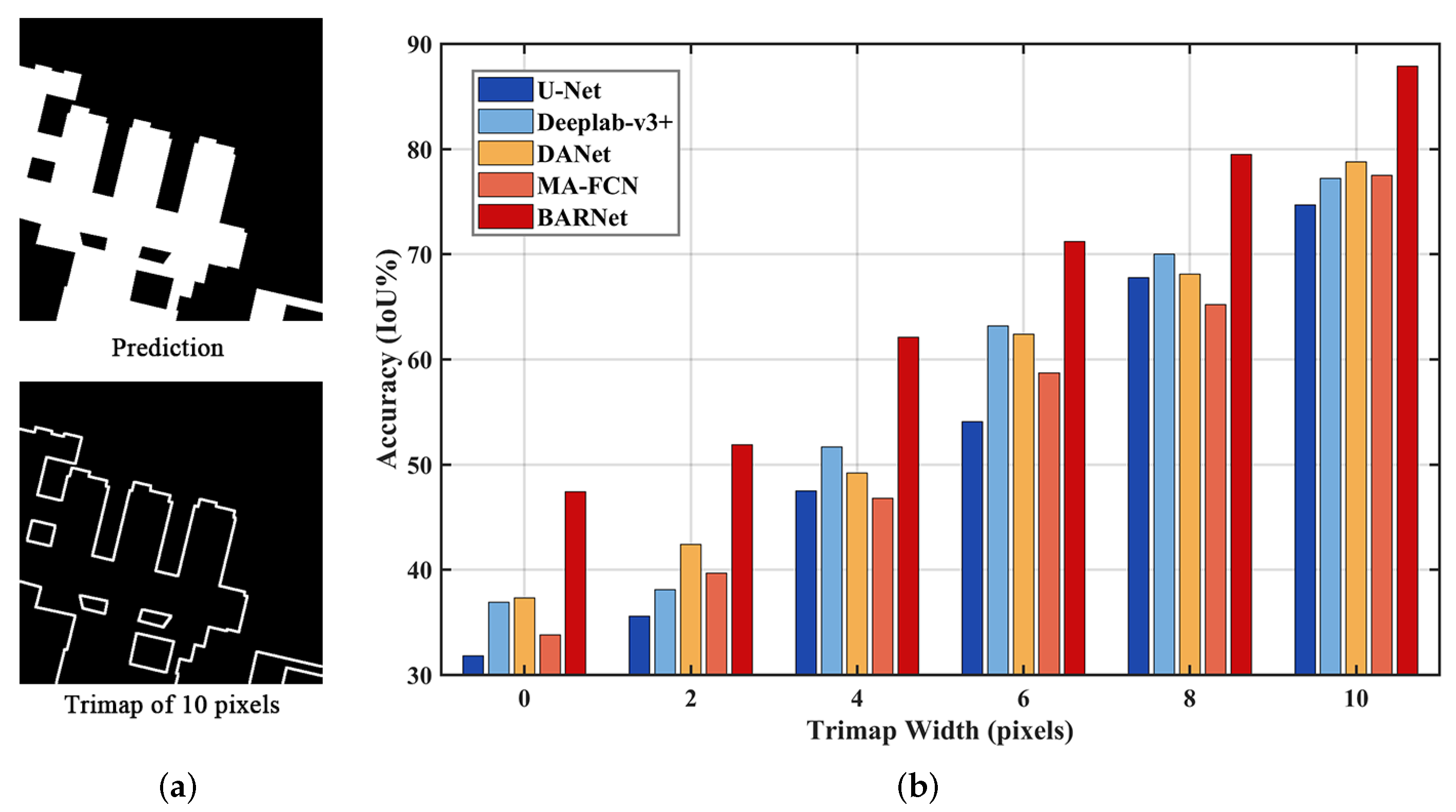
8) is termed the gradient information map, where a higher value stands for the probability of a pixel locating at the boundary, and vice versa. We extend the Laplacian operator to process the multidimensional tensor. An instance of using the Laplacian operator to obtain the building boundary is given in
Figure 5. With the yielded boundary maps
and boundary labels
, where
N,
H and
W are the batch size, image height and image width, respectively, the boundary refinement is defined as a cost minimum problem expressed by:
where
denotes the trainable parameters of the BARNet. For every single image, the weighted binary cross-entropy loss [
26] is employed to compute the boundary-enhanced loss
as:
where
and
represent the number of pixels in boundary and non-boundary regions, respectively.
The final Boundary-Aware (BA) loss
is defined as the addition of two losses, i.e.,
in which
is empirically set to 1 to balance the contribution of boundary-enhanced loss,
is the class weight calculated using the median frequency balance strategy [
1] and
and
denote the model predictions and corresponding labels, respectively.


