Article

Unsupervised Change Detection from Remotely Sensed Images Based on Multi-Scale Visual Saliency Coarse-to-Fine Fusion

1
School of Remote Sensing and Geomatics Engineering, Nanjing University of Information Science and Technology, Nanjing 210044, China
2
Jiangsu Power Design Institute, Co., Ltd. of China Energy Engineering Group, Nanjing 211102, China
3
School of Geography and Tourism, Qufu Normal University, Rizhao 276826, China
*
Author to whom correspondence should be addressed.
Remote Sens. 2021, 13(4), 630; https://doi.org/10.3390/rs13040630
Submission received: 7 January 2021 / Revised: 3 February 2021 / Accepted: 5 February 2021 / Published: 10 February 2021

Abstract

:
Unsupervised change detection(CD) from remotely sensed images is a fundamental challenge when the ground truth for supervised learning is not easily available. Inspired by the visual attention mechanism and multi-level sensation capacity of human vision, we proposed a novel multi-scale analysis framework based on multi-scale visual saliency coarse-to-fine fusion (MVSF) for unsupervised CD in this paper. As a preface of MVSF, we generalized the connotations of scale as four classes in the field of remote sensing (RS) covering the RS process from imaging to image processing, including intrinsic scale, observation scale, analysis scale and modeling scale. In MVSF, superpixels were considered as the primitives for analysing the difference image(DI) obtained by the change vector analysis method. Then, multi-scale saliency maps at the superpixel level were generated according to the global contrast of each superpixel. Finally, a weighted fusion strategy was designed to incorporate multi-scale saliency at a pixel level. The fusion weight for the pixel at each scale is adaptively obtained by considering the heterogeneity of the superpixel it belongs to and the spectral distance between the pixel and the superpixel. The experimental study was conducted on three bi-temporal remotely sensed image pairs, and the effectiveness of the proposed MVSF was verified qualitatively and quantitatively. The results suggest that it is not entirely true that finer scale brings better CD result, and fusing multi-scale superpixel based saliency at a pixel level obtained a higher F1 score in the three experiments. MVSF is capable of maintaining the detailed changed areas while resisting image noise in the final change map. Analysis of the scale factors in MVSF implied that the performance of MVSF is not sensitive to the manually selected scales in the MVSF framework.

Graphical Abstract

1. Introduction

As the fast development of imaging technology gives rise to easy access to image data, dealing with bi-temporal or multi-temporal images has been getting great concerns. Change detection (CD) is to detect changes from multiple images covering the same scene at different time phrases. Two main branches of the scholar community have been working on this problem, one is the computer vision (CV) and the other is remote sensing (RS). The former analyses the changes among multiple natural images or video frames to carry out further applications, such as object tracking, visual surveillance, and smart environments, etc. [1]. By contrast, the latter is engaged in obtaining the spatiotemporal changes of geographical phenomena or objects on the earth’s surface, such as land cover/use change analysis, disaster monitoring and ecological environment monitoring, etc. CD based on RS images usually undergoes more difficulties than natural images because of the intrinsic characteristics of various RS data sources, including multi/hyper-spectral (M/HS) images, high spatial resolution (HSR) images, synthetic aperture radar (SAR) images and multi-sources images. For example, the M/HS images contain more detailed spectral information, which makes it possible to detect various changes of geographical objects with particular spectral characteristic curves. Nevertheless, this profit comes at the cost of an increasing CD complexity due to the high dimensionality of M/HS data [2]. CD from HSR images can benefit from the fine representation of the geographical world with high spatial resolution, and more accurate CD results could be obtained. However, the consequent decrease of intra-class homogeneity and huge amount of noise have to be seriously considered. SAR imaging is an active earth observation system with day and night imaging capability regardless of the weather conditions. Since the inherently existed speckle noise degrades the quality of the SAR images, CD from SAR images also needs to withstand the effects of noise [3].
Generally, CD from remotely sensed images is aimed to obtain a change map (CM) indicating the changed areas with a binary image. The CD methods can be mainly classified as two groups including supervised CD and unsupervised CD. To learn the accurate underlying mode of ‘change’ and ‘no-change’, the supervised CD needs a huge amount of ground truth samples with high quality, which is usually time-consuming and labor-intensive. In contrast, the unsupervised CD has been getting more popular because of leaving the procedure of training data labelling. This paper accordingly focuses on the discussion of unsupervised CD.
Unsupervised CD is to make labeling decisions according to the understanding of data itself rather than being driven by labeled data. Statistical machine learning has been widely applied to CD problems. A classic work from Bruzzone L. and Prieto D.F. [4] proposed two CD methods for analysing the DI of the bi-temporal images automatically under a change vector analysis (CVA) framework. The two methods were based on the assumption that the samples from the DI are independent or not. One is an automatic thresholding method according to the Gaussian mixture distribution model and Bayes inference (noted as EM-Bayes thresholding). The other is a post processing method considering the contextual information modeled by Markov random field. Subsequently, many researches have been devoted to finding a more proper threshold, such as histogram thresholding [5] and adaptive thresholding [6], or modeling more accurate context information such as fuzzy hidden Markov chains [7]. Clustering is another commonly used technique in CD. Many clustering algorithms incorporated with fuzziness [8,9] or spatial context information [10,11] have been proposed to alleviate the uncertainty problems in remote sensing and obtain more accurate clusters indicating as ‘change’ and ‘no-change’.
Since around 2000, object-based image analysis(OBIA) for remote sensing has grown rapidly. Accordingly, Object-based change detection(OBCD) has been studied widely [12]. The OBCD considers image segments as the analysis units to obtain object-oriented features such as texture, shape and topology features, which can be utilized in the objects comparison procedure. Compared with the pixel-based CD, OBCD performs better in dealing with high-resolution images [13]. However, how to get high-quality image segments and how to make segments from image pairs one-one corresponding and comparable has gotten more concerns than CD problem itself [12].
Seen from the development of CD techniques, image feature representation is one of the key factors that lead the technological progress. Specifically, in nearly a decade, deep learning has been widely applied in remote sensing researches. Deep features with high-level semantic information obtained by deep neural networks (DNN) has become an outstanding supplement to the manually designed features [14]. Zhange P. etc. [15] incorporated deep-architecture-based unsupervised feature learning and mapping-based feature change analysis for CD, in which the denoising autoencoder is stacked to learn local and high-level representation from the local neighborhood of the given pixel in an unsupervised fashion. In the work by Gong M. etc. [16], autoencoder, convolutional neural networks (CNN) and unsupervised clustering are combined to solve ternary change detection problem without supervision. More information about deep learning based CD can be found in the review article [3].
In this paper, we would like to take a fresh look at the CD procedure. We consider it as a visual process when people conduct CD artificially from remotely sensed images. Accordingly, we built a new unsupervised CD framework inspired by the characteristics of human visual mechanism. In the practical manipulation of CD map manually, people are able to focus on the changed areas quickly when they watch both the images repeatedly or in a flicker way. Then, detailed changes can be found and delineated if people put attention on the changed areas of various sizes. We consider this sophisticated visual procedure to be attributed to the visual attention mechanism and multi-level sensation capacity of the human visual system. Visual attention refers to the cognitive operations that allow people to select relevant information and filter out irrelevant information from cluttered visual scenes efficiently [17]. As for an image, the visual attention mechanism can help people focus on the region of interests efficiently while suppressing the unimportant parts of the image scene. The multi-level sensation capacity can help people incorporate the multi-level information and sense the muli-scale objects in the real world [18]. Inspired by this, we proposed a novel unsupervised change detection method based on multi-scale visual saliency coarse-to-fine fusion (MVSF), aiming to develop an effective visual saliency based multi-scale analysis framework for unsupervised change detection. The main contributions of this paper are as follows.
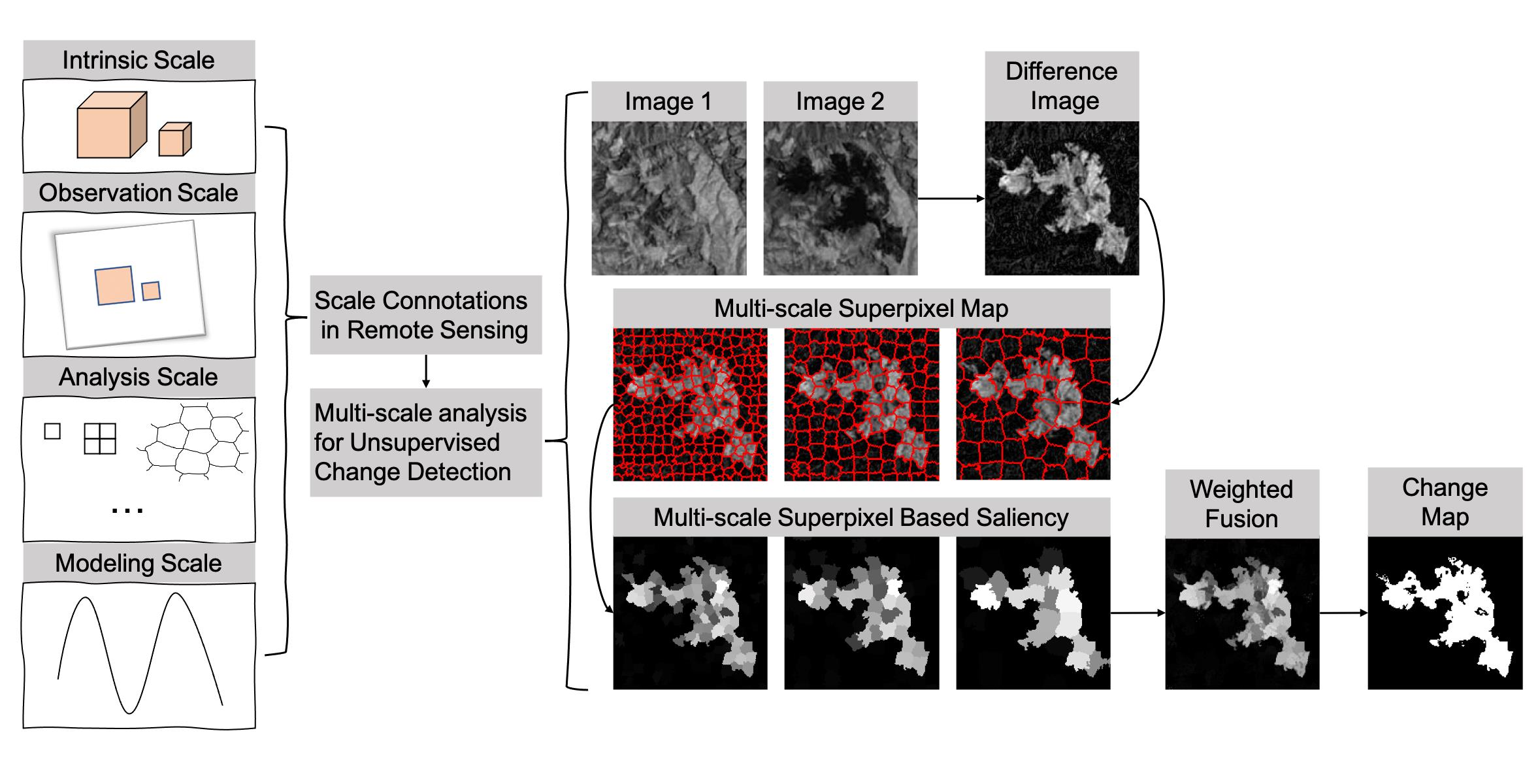
  • We generalized the connotations of scale in remote sensing as four classes including intrinsic scale, observation scale, analysis scale and modeling scale, which covers the remote sensing process from imaging to image processing.
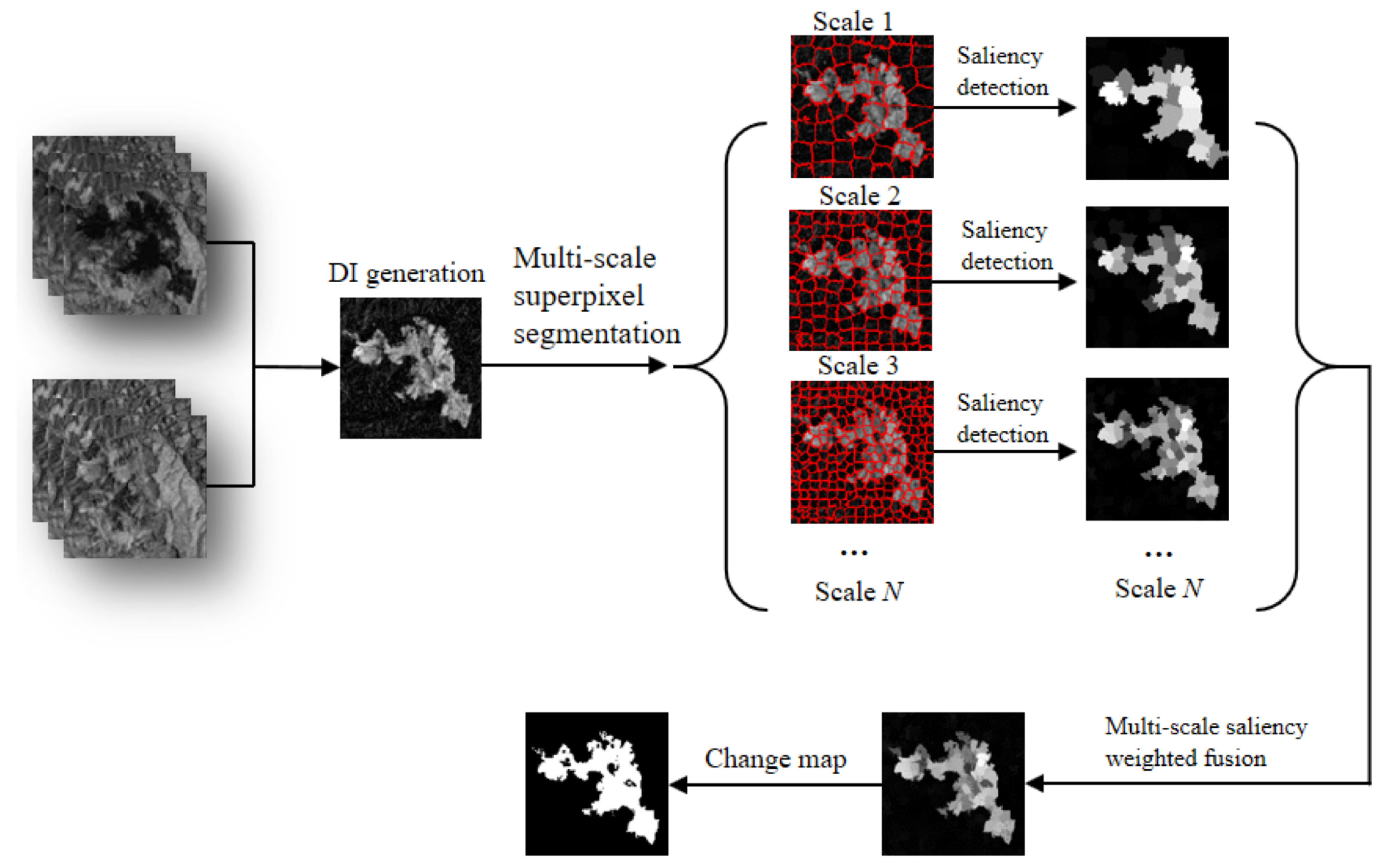
  • We designed the multi-scale superpixel based saliency detection to imitate the visual attention mechanism and multi-level sensation capacity of human vision system.
  • We proposed a coarse-to-fine weighted fusion strategy to incorporate multi-scale saliency information at the pixel level for noise eliminating and detail keeping in the final change map.
The remainder of this paper is organized as follows. We elaborate on the background and motivation of the proposed framework in Section 2. Section 3 introduces the technical process and mathematical description of the proposed MVSF in detail. Section 4 exhibits the experimental study and the results. Discussion is presented in Section 5. In the end, the concluding remarks are drawn in Section 6.

2. Related Background and Motivation

2.1. Multi-Scale Analysis in Remote Sensing

Scale is one of the most ambiguous conceptions. It has various scientific connotations in different disciplines. However, the underlying meaning is that scale is the degree of detail at which we observe an object or analyse a problem. In terms of remote sensing, we generalize the connotations of scale as four classes in this paper, including intrinsic scale, observation scale, analysis scale and modeling scale (See Table 1). These four classes are of a progressive relationship and cover the remote sensing process from imaging to image processing. As the intention of this paper, we will put emphasis on the analysis scale and modeling scale.
Analysis scale means the size of unit we use when dealing with RS images and image information detection. It has been considered a significant factor for the performance of CD [19]. The revolution of image analysis unit comes from the promotion of spatial resolution of RS images and development of image analysis technology. Individual pixel has been the basic unit for image analysis since the early use of RS images based on statistical characteristics. Then, spatial context information were further considered by using a window composed of neighbored pixels, named kernel. These two kinds of unit have been widely used in most of the traditional CD frameworks based on image algebra, image transformation, image classification and machine learning [12]. Specifically, some multi-scale analysis mathematical theories have been applied in the field of remote sensing, such as scale space theory [20] for image registration [21,22] and object detection [23,24]; wavelet for multi-scale feature extraction [25] and image fusion [26]; and fractal geometry for multi-scale image segmentation [27]. Using image objects as the units comes from the development of object-based image analysis technique(OBIA). Resulting from the various intrinsic scales of geographic entities in the world, it is difficult to define single or most appropriate scale parameter for segmentation to create the optimized objects with accurate boundaries. It means that the subsequent analysis usually endures the impacts of over-segmentation or under-segmention. Thus, multi-scale segmentation with varying scale paramters for multi-scale representation has been getting more and more popular with the development of OBIA [28,29]. Superpixel is a perceptually meaningful atomic region composed of a group of pixels with homogeneous features. Superpixel segmentation can normally obtain regular and compact regions with well-adhering boundaries compared with conventional image segmentation approaches. Thus, it greatly reduces the complexity of subsequent image analysis [30]. Compared with pixel and image object, superpixel has been considered as the most proper primitive for CD [19].

2.2. Superpixel Segmentation

There are many approaches to generate superpixels. They can be broadly categorized as either graph-based or gradient ascent methods [30]. In Ref. [30], the authors performed an empirical comparison of five state-of-the-art algorithms concentrating on their boundary adherence, segmentation speed and performance when used as a pre-processing step in a segmentation framework. In addition, they proposed a new method for generating superpixels based on K-means clustering, called Simple Linear Iterative Clustering (SLIC). SLIC has been shown to outperform existing superpixel methods in nearly every respect. Specifically, the zero parameter version of SLIC (SLICO) adaptively chooses the compactness parameter for each superpixel differently. SLICO generates regular shaped superpixels in both textured and non-textured regions, and this improvement comes with hardly any compromise on the computational efficiency. The only parameter required in SLICO is the manually set number of superpixels, which can be considered as the scale parameter under the interpretation of scale we made in Section 2.1. Detailed discussion on SLIC can be found in the work [30].

2.3. Visual Saliency for Change Detection

Visual saliency is originally studied in the field of neurobiology, aiming to understand the mechanism of visual behavior. Then, it was applied to computer vision for detecting salient region of an image. Visual saliency of an image reveals the obvious areas where a target of interest initially attracts the human eyes. This mechanism has spawned many bottom-up visual saliency detection methods [31,32]. Normally, they are designed by following the basic principles of human visual attention, such as contrast consideration and center prior, which means the salient region usually has a sharp contrast with the background and locates in the center of the image as well.
The strong visual contrast of changed areas in DI makes visual saliency suitable to guide the CD procedure [33]. In Table 2, we state the differences and similarities between saliency detection from natural images and CD from RS images. The direct relation between them is that they both need the consideration of contrast and integrity. Here, the integrity consideration means all the saliented objects (changed areas) from the given image scene need to be discovered and all parts that belong to a certain salient object (changed area) should be highlighted [34]. However, CD does not need to consider center prior, because the changed areas may spread any place of an image. Even so, many previous works [33,35,36] have proven contrast based saliency detection to be efficient for locating the changed areas fast while suppressing the interfered information in unchanged areas.
As described above, this paper introduces multi-scale superpixel based saliency detection for multi-scale analysis of DI. The generated multi-scale saliency maps will finally be integrated by a proposed weighted fusion strategy at a pixel level. The mathematical description of MVSF is presented in detail in the following section.

3. Methodology

Figure 1 gives an illustration of the proposed MVSF. Firstly, the DI is generated with CVA method. Then, we consider superpixels as the basic units to decrease the effects of image noise and keep the changed areas structured with good boundary adherence [30]. Specifically, the scale parameter are set with different values to obtain multi-scale segmentation results during superpixel segmentation. Third, global contrast based saliency detection at superpixel level is conducted to highlight the changed areas while suppressing the unchanged areas. Finally, a coarse-to-fine multi-scale saliency fusion strategy is proposed to keep the changed areas of varying sizes well-structured while retaining detailed changes. In the end, the final change map can be generated by simple clustering or thresholding method.

3.1. Difference Image Generation and Multi-Scale Superpixel Segmentation

DI is normally obtained by subtracting the corresponding components of bi-temporal images with an L2 norm compression for each pixel. This procedure can also be applied to feature maps after feature detection from the bi-temporal images. Given two co-registered bi-temporal images X 1 and X 2 with same size R × C × B , let [ F 1 1 , F 2 1 , , F N 1 ] and [ F 1 2 , F 2 2 , , F N 2 ] be the feature maps with size R × C × N after image feature detection from X 1 and X 2 . The DI, noted as X D can be generated by:
X D = n = 1 N ( F n 2 F n 1 ) 2
where n = 1 N here is an element-wise processing for the change vector of each pixel. X D preserves the main properties of the changes despite the compression of the change vector size from [R, C, N] to [R, C, 1] [37]. Pixel values of X D indicate the magnitude of the changes.
After DI generation, we chose SLICO to segment the DI into superpixels because of its high efficiency of operation and high quality of results [30]. Specifically, the only parameter of SLICO is the desired number of approximately equally sized superpixels. As the remote sensing image is a reflection of the multi-scale objects on the earth, the DI also conveys changed areas with various sizes. It is not reasonable to use the segmentation result of DI at a single scale, because it can not describe the multi-scale objects in the image accurately and breaks the rules of the multi-level visual sensation of human vision. Thus, we use multi-scale superpixel segmentation of DI to detect multi-scale change information. The CD results will be finally promoted by a coarse-to-fine fusion process we proposed, which will be introduced in detail in Section 3.3.
Note the multi-scale superpixel maps generated from DI by SLICO as [ S 1 , S 2 , , S N ] , in which N is the number of scales we adopted. For superpixel map at ith scale, namely, S i ( i [ 1 , N ] ), the approximate size of S i is therefore R × C / K i pixels, in which K i is the scale parameter set for generating S i .

3.2. Saliency Detection at Superpixel Level

In terms of superpixel based saliency detection, the global contrast and prior of spatial distribution of the salient region is commonly considered [32,38,39]. As there is no prior information of the spatial distribution of changed areas, we simply used global contrast to obtain the saliency map for each scale regardless of the spatial location. The saliency of each superpixel is caculated by averaging the global contrast with all the other superpixels. Note s i j is the jth superpixel at ith scale in S i , m i j is the average spectral value of the pixels in s i j . The saliency of s i j , noted as c i j can be obtained by,
c i j = k = 1 K i ( | m i j m i k | ) / K i
in which j , k [ 1 , K i ] and j k . The multi-scale saliency maps, noted as [ C 1 , C 2 , , C N ] , can be obtained by calculating the saliency of all the superpixels at all scales. For the pixels in a certain superpixel, we consider that they share the same saliency value with the superpixel they belong to.

3.3. Multi-Scale Saliency Coarse-to-Fine Fusion

The generated saliency maps reveal the possibility of changes of a superpixel at different scales. However, as the size of changed areas varies all over the image, over-segmentation and under-segmentation may happen at a single scale when the superpixel size is smaller or larger than the changed areas. This will lead to some false alarms or omissions in the CD result. To maintain the details of changed areas while suppressing the noise, a weighted fusion strategy was designed to incorporate multi-scale saliency at pixel level. Note the saliency map at i t h scale as C i = { c ( r , c ) i | r [ 1 , R ] , c [ 1 , C ] } , in which c ( r , c ) i is the saliency value of pixel ( r , c ) in C i and shares the same saliency value of the superpixel it belongs to. Then, the proposed multi-scale weighted saliency fusion at pixel level can be formulated as
C fused = i = 1 N w ( r , c ) i c ( r , c ) i i = 1 N w ( r , c ) i ( r [ 1 , R ] , c [ 1 , C ] )
in which, C fused is the fused saliency map from multi-scale saliency maps [ C 1 , C 2 , , C N ] , w ( r , c ) i is the weight of fusion for the pixel at scale i, the denominator i = 1 N w ( r , c ) i is the normalization factor. Specifically, the weight of fusion for pixels at different scales were designed out of the following concerns. Firstly, the weight should be decreased if the superpixel, where the pixel belongs to, has a higher heterogeneity. High heterogeneity normally means under-segmentation happens, so we give a penalty to the pixel for the uncertainty of sharing the same saliency with the superpixel it belongs to. In such cases, we further decrease the weight if the spectral distance between the pixel and the superpixel (the average spectral value of the pixels in the same superpixel) is larger. The weight item w ( r , c ) i can be finally formulated as,
w ( r , c ) i = 1 v i j · d ( x ( r , c ) , x i j ¯ )
in which v i j is the spectral variance of all the pixels that belong to the same superpixel s i j , and it represents the degree of heterogeneity. d ( x ( r , c ) , x i j ¯ ) is the spectral distance between pixel x ( r , c ) and the superpixel it belongs to. With the fused saliency map, the changed areas are much more highlighted and unchanged areas are suppressed. Then the final change map can be generated by simple thresholding or clustering method.

4. Experimental Study

4.1. Datasets

Three datasets from multiple sensors were employed in our experimental study. The first dataset consists of bi-temporal Landsat Enhanced Thematic Mapper Plus(ETM+) images with a section of 512 × 512 obtained on April 2000 and May 2002. Figure 2a,b shows the fourth band of the images and they reveal the changes after a forest fire in Mexico. The Second dataset is composed of two Landsat-5 Thematic Mapper (TM) images with a size of 300 × 412 , captured at September 1995 and July 1996. Band 4 of the bi-temporal images are illustrated in Figure 2d,e, and they display the changes of the Mediterranean Sardinia, Italy. The third dataset (Figure 2g,h) is a section ( 350 × 290 ) of two Radarsat-1 SAR images covering Ottawa city, Canada, and they show the changes caused by flooding during July to August 1997. The areas in the three datasets have detailed changes with various sizes and noise interference, which can reflect the MVSF performances during the experiments. Figure 2c,f,i are the corresponding reference change maps of the three datasets. They were all generated by manual visual interpretation of the changes.

4.2. Implementation Details and Evaluation Criteria

In the experimental study, the implementation of the algorithms and accuracy evaluation was conducted with Python 3.7 in an integrated development environment called PyCharm. For each dataset, the DI was generated by utilizing the original spectral feature for simplicity. The superpixel segmentation was implemented by using the image processing Python package named scikit-image [40]. The scale parameter K was set manually with K = 500 , 1000 , 2000 for multi-scale analysis in the MVSF framework, which is simply represented as scale 500, scale 1000 and scale 2000 in the following text for convenience.
We adopted the widely used evaluation criteria by comparing the CD result with the reference change map, in order to analyse the performance of the proposed method quantitatively. False negative (FN) denotes the number of pixels which are classified into the unchanged regions but changed in the reference change map, while false positive (FP) represents the number of pixels which are classified into the changed regions but unchanged in the reference change map. True negative (TN) denotes the number of pixels which are correctly classified into the unchanged, while true positive (TP) is the number of pixels which are correctly classified into the changed. Then, four indexes can be calculated to valuate the CD results, including the average correct classification rate (ACC) ACC = (TN + TP)/(TN + TP + FN + FP), Precision = TP/(TP + FP), Recall = TP/(TP + FN) and F1 score= 2 × Recall × Precision/(Recall + Precision).

4.3. Effects of Single Scale of Superpixel Segmentation

The scale parameter in the proposed MVSF is the number of superpixels we set manually, which determines the size of a superpixel. To verify the performance of superpixel segmentation of RS images at different scales, we took the Mexico dataset for example. For the convenience of illustration, Figure 3 presents subsets of the superpixel segments boundaries covering DI with scales at 500, 1000 and 2000, in which the boundaries between the adjacent superpixels are delineated using red lines. As we can see, the generated superpixels by SLICO at each single scale are of the similar size and generally have well-adhering boundaries. This will facilitate the following process of CD. Segments at finer scale perform better at describing the tiny changed areas with accurate boundaries (seen from the areas in the yellow circles of Figure 3a–c). However, CD at finer scale not only brings higher cost of time but also has a risk of introducing the noise.

4.4. Valuation of the Performance of MVSF

To verify the effectiveness of the proposed MVSF, we conducted three experiments on Mexico dataset, Sardinia dataset and Ottawa dataset, respectively. For each experiment, we illustrated the multi-scale fused saliency map and the CD result by MVSF. As comparisons, we also present the superpixel saliency maps at each scale and the corresponding change maps by applying K-means. Besides, EM-Bayes thresholding [4] and K-means clustering on DI were carried out and the results were presented. All the CD results were evaluated quantitatively by the foregoing criterias.

4.4.1. Experiment on Mexico Dataset

Figure 4 presents the experimental results of Mexico dataset. Figure 4a–c is the superpixel based saliency map at scale 500, 1000 and 2000, respectively. The number of generated superpixels is 484, 1024, 2181 for each corresponding scale. It is obvious that superpixel based saliency inherits the advantages of SLICO superpixel segmentation. The salient region, which indicates the high possibility of changed areas, has kept good boundaries. It also helps to highlight the changed areas and suppress the noise in the unchanged background. Moreover, the scale effects we discussed before have embodied the saliency maps at different scales. Figure 4d is the fused saliency map by the proposed weighted fusion strategy of Figure 4a–c. The fused saliency map has shown a finer description of saliency, which gives more details while suppressing the noise because of the weighted integration of multiple scale saliency information at a pixel level. This can be further proved by Figure 4e–h, which show the change maps by K-means on Figure 4a–d. Figure 4i,j shows the change maps by K-means and EM-Bayes on DI, respectively. As we can see, they both suffer from the noise seriously. By comparison, Figure 4h, namely the change map by MVSF, has given the best CD result thanks to the superpixel based saliency and weighted multi-scale fusion strategy we proposed.
Table 3 presents the quantitative comparison analysis of MVSF. In terms of change map generated from superpixel based saliency map at scale 500, 1000, 2000, we found that it obtained the highest F1 score (0.884) at scale 1000 than the other two scales (0.866 at scale 500 and 0.865 at scale 2000). This suggests it is not entirely true that finer scale brings higher CD accuracy. The reason would be the saliency map at finer scale may mix with noise even though it supplies more details. By contrast, the proposed MVSF performed best with the highest F1 score at 0.890 and it exceeds the F1 score of K-means and EM-Bayes as well. Moreover, MVSF obtained the highest precision at 0.971. This is because K-means and EM-Bayes has lots of false alarms as we can see from Figure 4f,i.

4.4.2. Experiment on Sardinia Dataset

The experimental results of Sardinia dataset are given in Figure 5. Figure 5a–c is the superpixel based saliency map at scale 500, 1000 and 2000, in which the number of generated superpixels is 494, 998, 1955, respectively. Figure 5d is the saliency map after multi-scale saliency weighted fusion of Figure 5a–c. Figure 5e–h shows the change maps by K-means on Figure 5a–d. Figure 5i–j shows the change maps by K-means and EM-Bayes on DI, respectively. In terms of the qualitative analysis, K-means and EM-Bayes both failed to overcome the serious noise problem. By contrast, superpixel based saliency helps to detect the changed areas with a robust ability of eliminating the noise. However, the utility of superpixels would recede with the down scaling of the superpixels for the sake of detecting more detailed information. As we can see from Figure 5g, noise starts to emerge when the scale is 2000. Among all the change maps, MVSF performed the best although it has obvious miss detections compared with the reference change map. This is because of a compromise between details keeping and noise eliminating. If we fuse more finer scales of the scaliency maps, the noise would pollute the final change map gradually.
Table 4 presents the quantitative comparison analysis of MVSF. For the performance of the single scale, scale 1000 obtained the higher F1 score at 0.844 than the other two scales (0.809 at scale 500 and 0.828 at scale 2000). Meanwhile, MVSF obtained the highest F1 score at 0.855. The F1 score of K-means and EM-Bayes is only 0.739 and 0.559, respectively. This is because the change map by K-means and EM-Bayes have large number of false detections, and the precision of them have been pulled down drastically to 0.637 and 0.399, respectively.

4.4.3. Experiment on Ottawa Dataset

Figure 6 presents the experimental results of Ottawa dataset. The number of generated superpixels is 524, 1015, 2041 at each corresponding scale of 500, 1000 and 2000. Figure 6a–c is the superpixel based saliency map at different scales. Figure 6d is the final saliency map by fusing weighted multi-scale saliency maps (Figure 6a–c). Figure 6e–h presents the change maps by K-means on Figure 6a–d. Figure 6i,j shows the change maps by K-means and EM-Bayes on DI, respectively. Table 5 presents the quantitative comparison analysis of MVSF. The Ottawa dataset is composed of two SAR images with heavy speckle noise interference. As a result, the change maps by K-means and EM-Bayes on DI seem to be insufferable with large amount of noise (Seen from Figure 6i,j), and the corresponding F1 score is only 0.669 and 0.485 respectively. By contrast, change map by MVSF outperformed the others qualitatively and quantitatively with F1 score at 0.739. It suggests that MVSF has a robust ability of suppressing noise.

4.4.4. Analysis of the Scale Factors

For multi-scale analysis in remote sensing, it is normally difficult to determine the optimal scales. The selection of scales for multi-scale saliency fusion is worthy to analyse in the MVSF framework. In the forgoing experimental study, we segmented the DI at three scales, namely scale = 500, 1000, 2000, and the obtained change maps of the three datasets have shown better performance after the designed pixel level multi-scale saliency fusion. In this subsection, we will further analyse the effects of scale factors to the change detection results.
We consider five scales for analysis, including scale = 500, 1000, 2000, 4000, 8000, noted as 0.5, 1, 2, 4, 8 ( × 10 3 ) for convenience. Then, the F1 scores of CD results in different fusion cases were explored. Table 6 presents the different fusion cases and scale permutations we applied in the experiment. Figure 7a–c illustrates the corresponding F1 scores of the change maps by fusing two scales, three scales and four cases, respectively. The F1 scores of the change map by fusing all the five scales for the Mexico dataset, Sardinia dataset and Ottawa dataset is 0.874, 0.851 and 0.753, respectively.
Seen from Figure 7a–c, the F1 score curves of the change maps from the three datasets fluctuate in a very small range for each fusion case. The maximum fluctuated range is 0.035, appeared in the F1 score curve of fusing two scales for the Ottawa dataset (the green curve in Figure 7a). Besides, the F1 score curve seems to be more stable with more scales are fused, according to the F1 score curves of the change maps by fusing two scales, three three and four scales. Figure 8 presents the average F1 scores of fusing various number of scales. It shows that the average F1 scores of the three fusion cases for all the three datasets are almost identical, which is around 0.875 for Mexico dataset, 0.850 for Sardinia dataset and 0.752 for Ottawa dataset, respectively. Overall, the analysis of the results implies that the accuracy of the CD result is not sensitive to the scale factors. It clarifies the confusion of choosing scales to apply the MVSF framework for CD. We believe that it is more appropriate to choose three scales for multi-scale saliency fusion in a balanced consideration of the performance stability and the calculation cost.

5. Discussion

For traditional unsupervised CD, balance of the removing noise and maintaining multi-level change details has been a headache for most CD algorithms. For example, the pixel based CD, which considers pixels as the basic analysis units, has to develop novel feature descriptors to cope with noise problem. The object based CD is based on the comparison of the segmented objects between different image phases. The results usually depend on the quality of image segmentation, and it is also difficult to determine the optimal segmentation scale. Therefore, multi-scale analysis of remote sensing image is of great importance for CD. However, as far as we know, there is a lack of clear generalization of the concept ‘scale’ in remote sensing, and novel multi-scale analysis framework for CD is still required to be developed further.
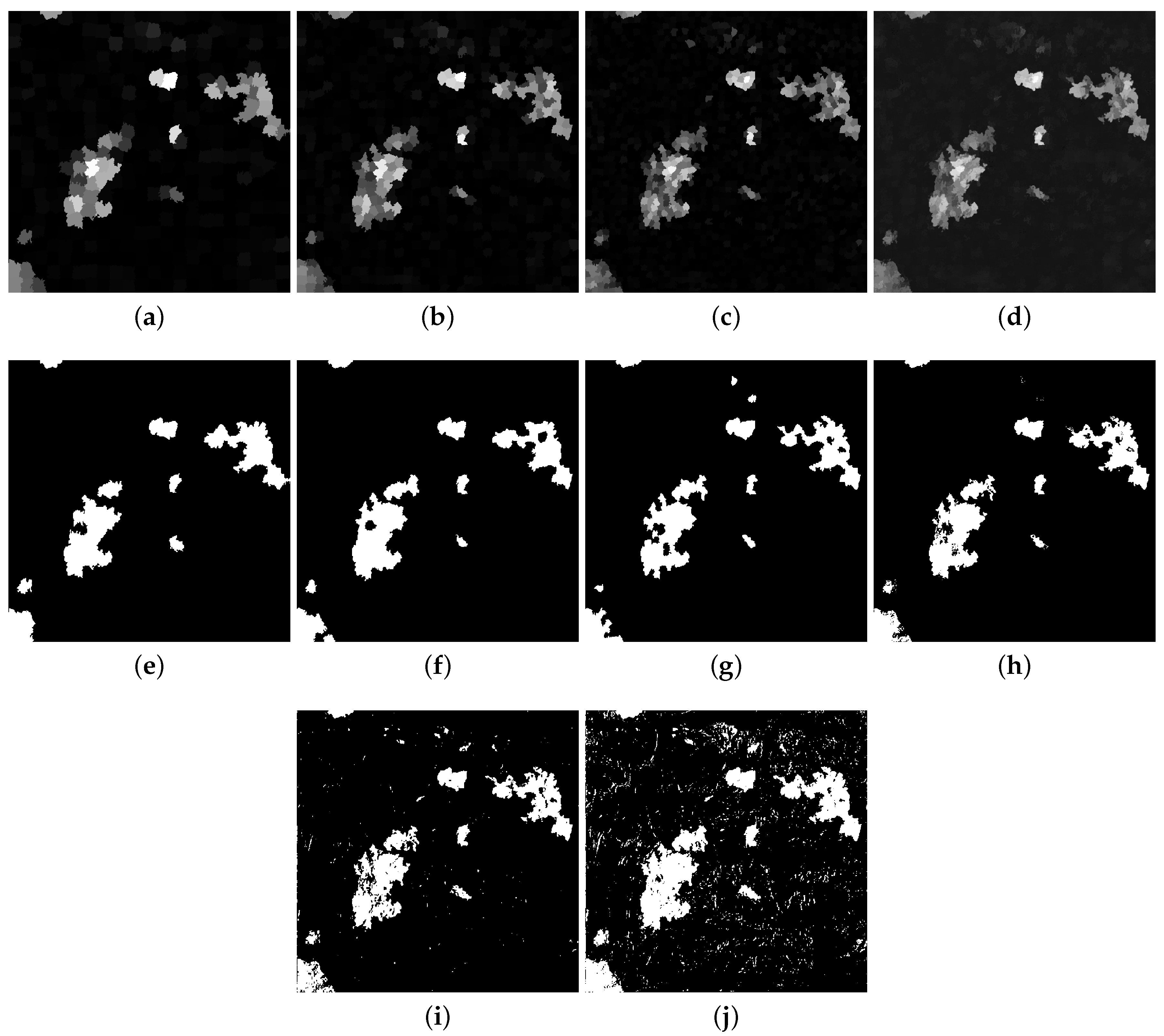
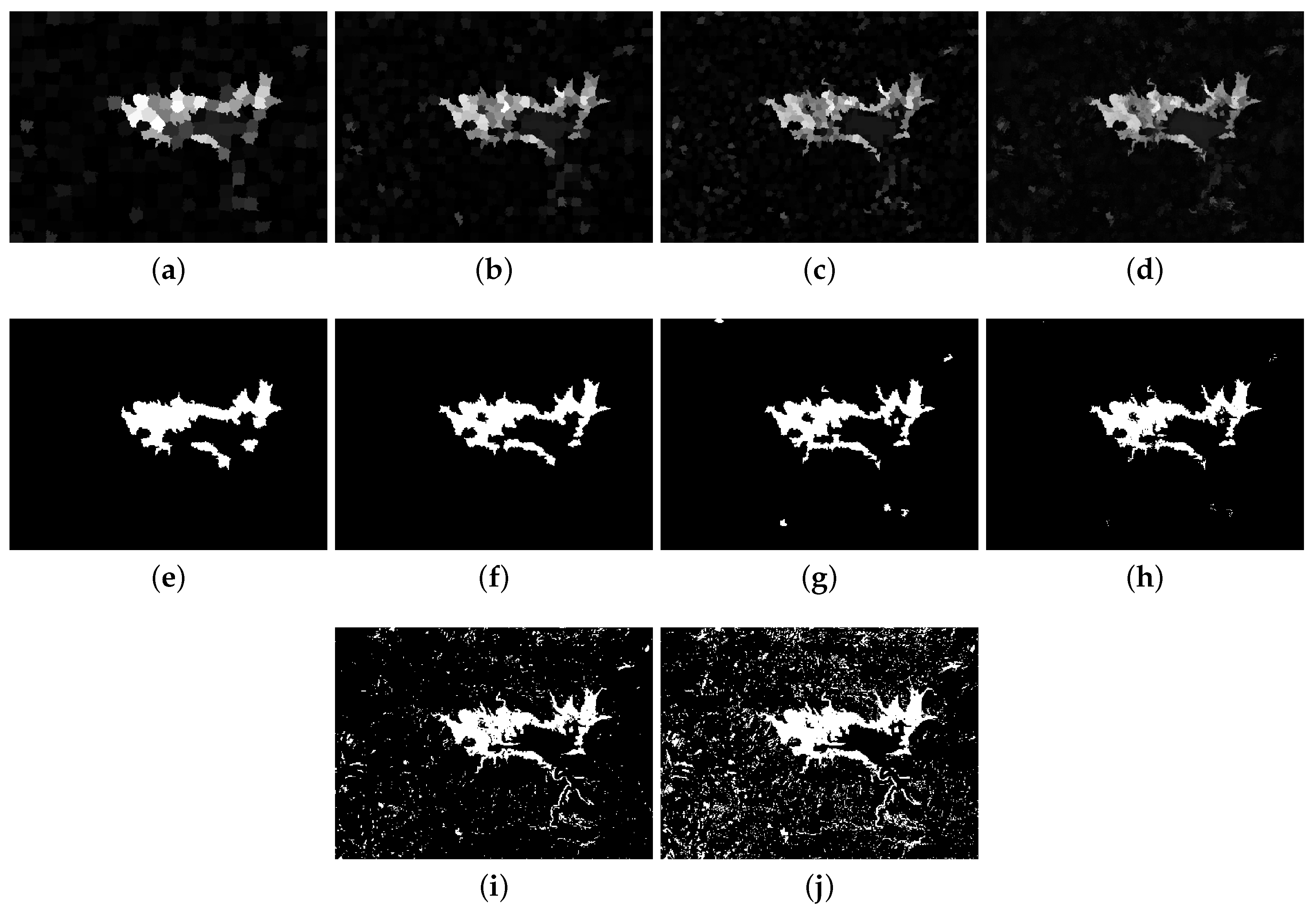
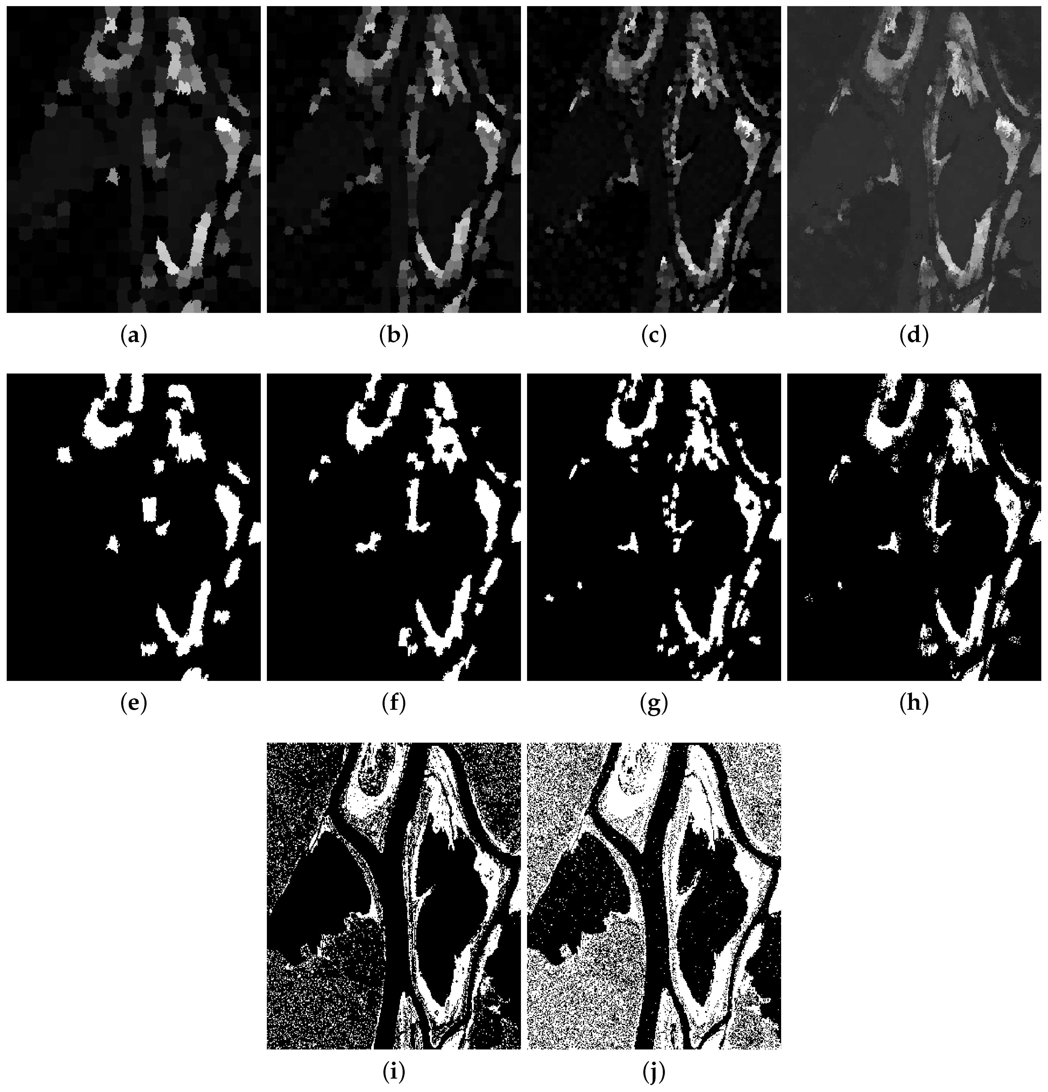
In this paper, we generalized the connotations of scale in the field of remote sensing as intrinsic scale, observation scale, analysis scale and modeling scale, which covers the remote sensing process from imaging to image processing. From views of analysis scale and modeling scale, We further proposed a novel unsupervised CD framework based on multi-scale visual saliency coarse-to-fine fusion, inspired by the visual attention mechanism and the multi-level sensation capacity of human vision. Specifically, superpixel was considered as the primitives for generating the multi-scale superpixel based saliency maps. A coarse-to-fine weighted fusion strategy was also designed to incorporate multi-scale saliency information at a pixel level.
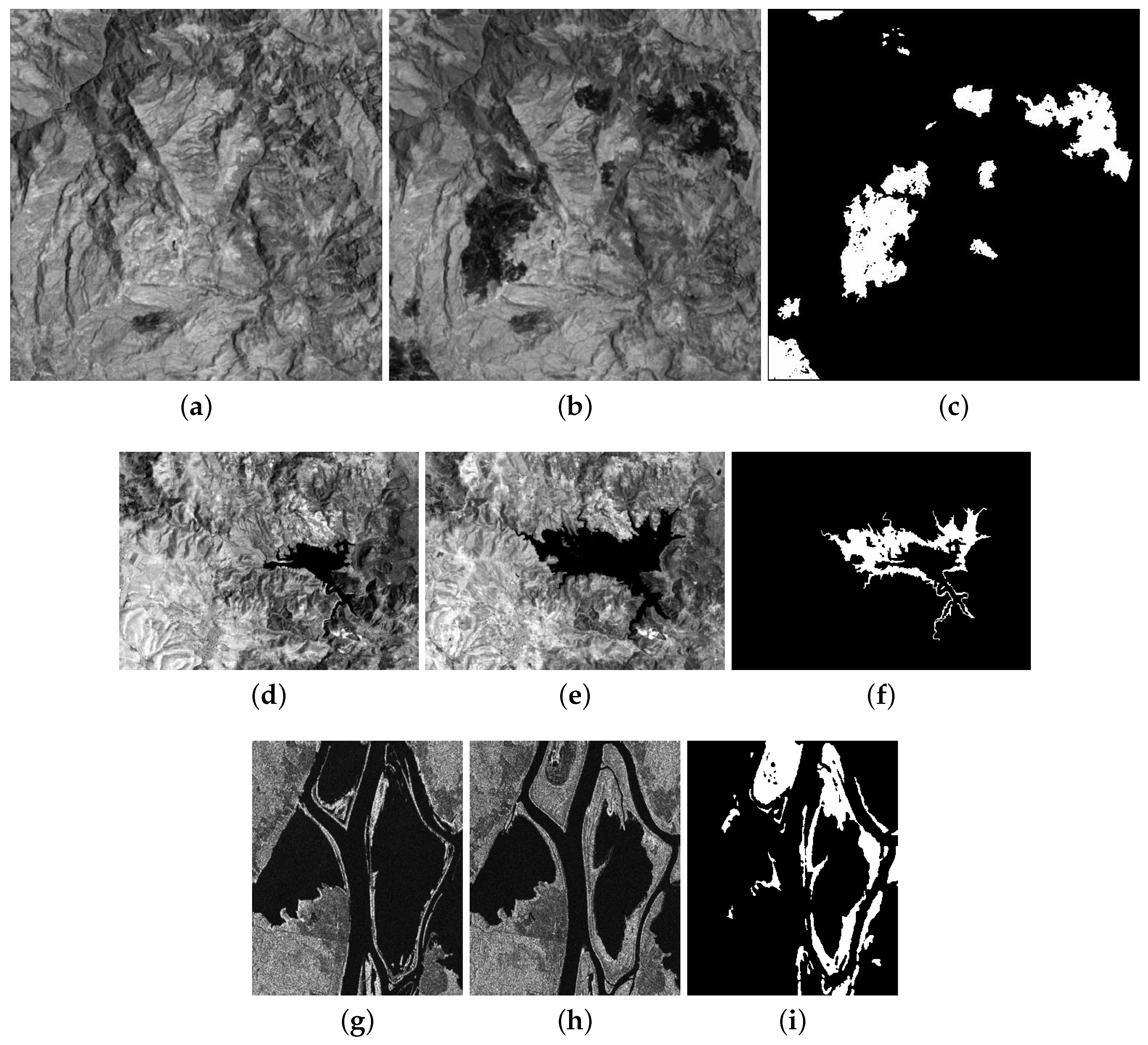
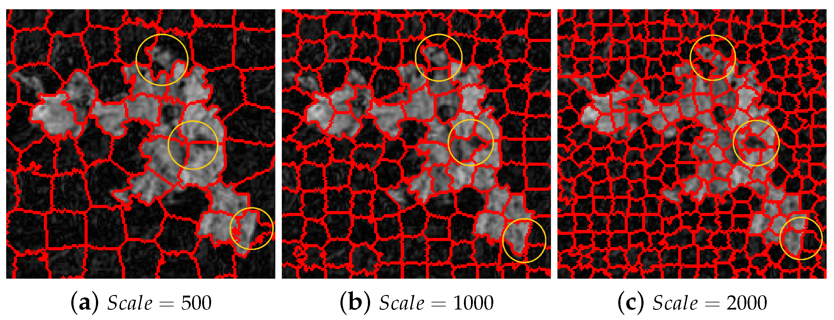
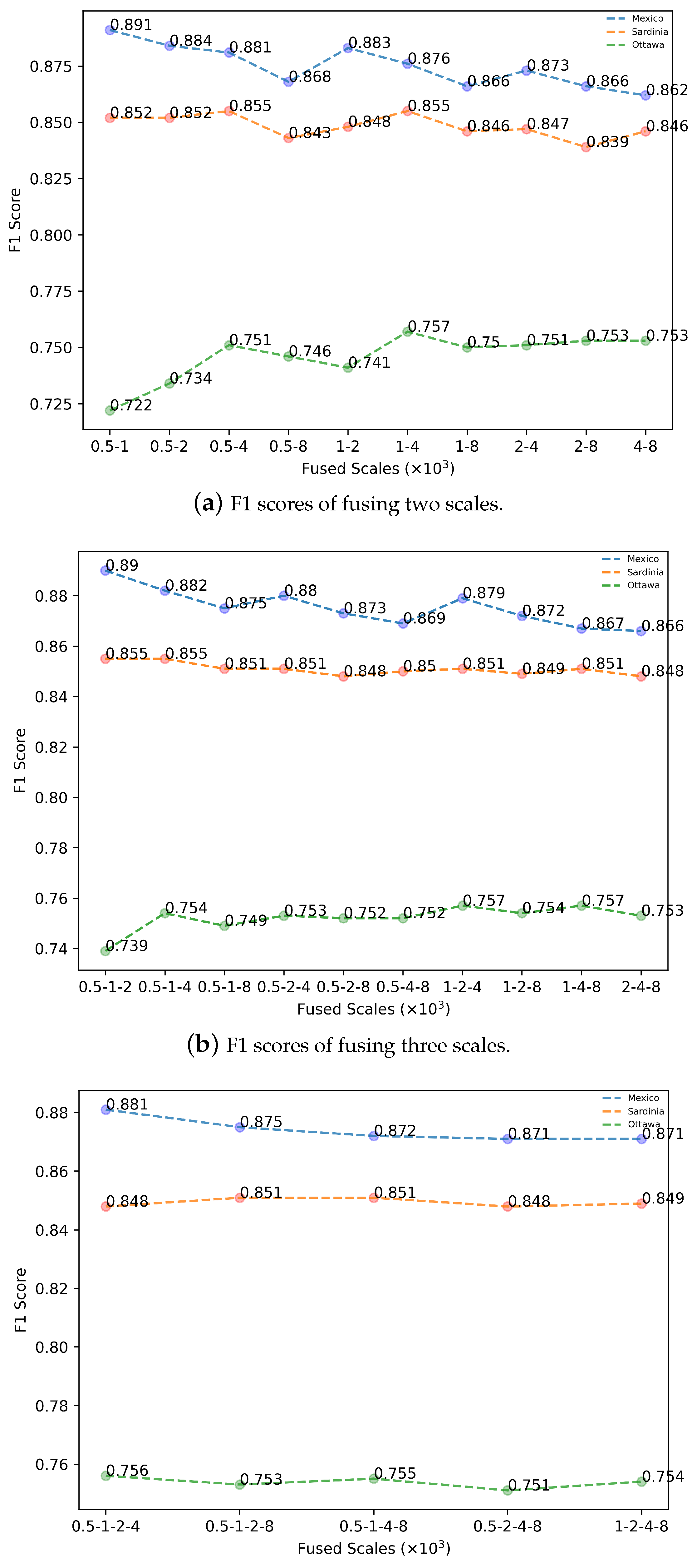
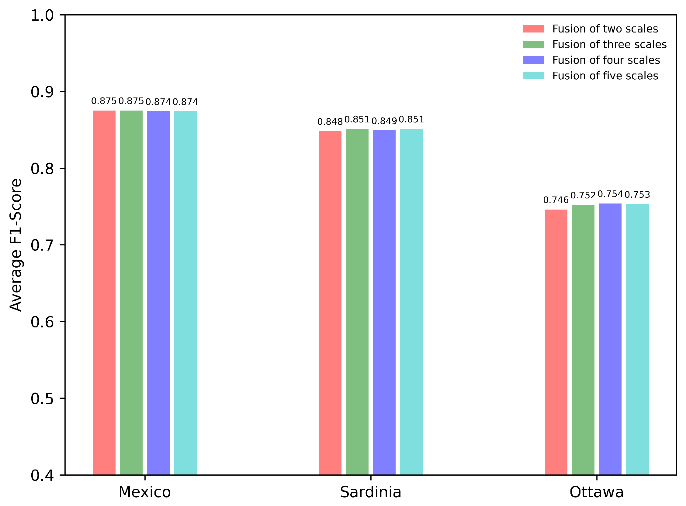
The effectiveness of the proposed MVSF was comprehensively examined by the experimental study on three remote sensing datasets from different sensors. The MVSF has shown its superiority through the qualitative and quantitative analysis against the popular K-means and EM-Bayes. On one hand, MVSF performed a robust ability of suppressing noise, although there is no utilization of high-level features in the experiments. One of the reasons is that generating superpixels can be recognised as a denoising process. The other reason lies in that the visual saliency itself has abilities of suppressing the background information. On the other hand, the proposed multi-scale saliency weighted fusion at the pixel level can incorporate multi-level change information, and maintain the change details well. Overall, the superiority of MVSF makes it applicable to images with multiple changes of various sizes and noise interference. In addition, we also analysed the scale factors in the MVSF framework, and the results implied that the accuracy of CD results by MVSF is not sensitive to the manually chosen scales. It means the performance of MVSF is stable against the scale factors.
It should be noted that there exist potential limitations of the MVSF framework. First, for the four scale connotations we generalized, we has already incorporated the analysis scale and modeling scale in the multi-scale analysis framework. However, an excellent multi-scale analysis framework for CD could also deal with the RS images with multiple observation scales, namely spatial resolution or spectral resolution. That is what we will work on in the future. Second, as we referred before, this work was inspired by the visual attention mechanism and multi-level visual sensation capacity of human vision. With the development of the recognition of human vision mechanism, advanced visual attention algorithm and multi-scale fusion method could be applied in the MVSF framework to improve the CD performance.

6. Conclusions

This paper proposed a novel multi-scale analysis framework for unsupervised CD based on multi-scale visual saliency coarse-to-fine fusion. To imitate the visual attention mechanism and multi-level sensation capacity of human vision, the proposed MVSF produces the multi-scale visual saliency at the superpixel level, and they are subsequently incorporated by a weighted coarse-to-fine fusion strategy at the pixel level. The performance of MVSF was examined qualitatively and quantitatively by an experimental study on three remotely sensed images from different sensors. The results indicated that the MVSF is capable of maintaining the detailed changed areas while resisting image noise in the final change map. In addition, the performance of MVSF is robust to the scale factors chosen manually in the multi-scale analysis framework. In the future, we will incorporate the observation scale into the multi-scale analysis framework and exploit the potentials of dealing with RS images with various spatial or spectral resolution for MVSF. The MVSF framework could also be further improved by more advanced visual attention algorithm and multi-scale description method with the progressive understanding of human vision.

Author Contributions

P.H. conceived the study and wrote the draft manuscript. X.Z. helped to refine the methodology and experiments. Y.S. gave constructive comments and revised the manuscript synthetically. L.C. proofread the paper and gave valuable suggestions. All authors have read and agreed to the published version of the manuscript.

Funding

This research was funded in part by the Natural Science Foundation of Jiangsu Province (under grant number: BK20190785); in part by the Startup Project for Introducing Talent of NUIST (under grant number: 2018r031); in part by the National Natural Science Foundation of China (under grant number: 41471312); in part by the Shandong Provincial Natural Science Foundation (under grant number: ZR2019BD045).

Institutional Review Board Statement

Not applicable.

Informed Consent Statement

Not applicable.

Data Availability Statement

Not applicable.

Conflicts of Interest

The funders had no role in the design of the study; in the collection, analyses, or interpretation of data; in the writing of the manuscript, and in the decision to publish the results.

Abbreviations

The following abbreviations are used in this manuscript:
CDchange detection
CMchange map
CNNconvolutional neural networks
CVcomputer vision
CVAchange vector analysis
DNNdeep neural networks
DIdifference image
ETM+Landsat Enhanced Thematic Mapper Plus
FNfalse negative
FPfalse positive
HSRhigh spatial resolution
RSremote sensing
M/HSmulti/hyper-spectral
MVSFmulti-scale visual saliency coase-to-fine fusion
OBIAobject-based image analysis
OBCDobject-based change detection
SARsynthetic aperture radar
SLICsimple linear iterative clustering
SLICOzero parameter version of SLIC
TMThematic Mapper
TNtrue negative
TPtrue positive

References

  1. Goyette, N.; Jodoin, P.; Porikli, F.; Konrad, J.; Ishwar, P. Changedetection.net: A new change detection benchmark dataset. In Proceedings of the 2012 IEEE Computer Society Conference on Computer Vision and Pattern Recognition Workshops, Providence, RI, USA, 16–21 June 2012; pp. 1–8. [Google Scholar]
  2. Marinelli, D.; Bovolo, F.; Bruzzone, L. A novel change detection method for multitemporal hyperspectral images based on binary hyperspectral change vectors. IEEE Trans. Geosci. Remote Sens. 2019, 57, 4913–4928. [Google Scholar] [CrossRef]
  3. Shi, W.; Zhang, M.; Zhang, R.; Chen, S.; Zhan, Z. Change Detection Based on Artificial Intelligence: State-of-the-Art and Challenges. Remote Sens. 2020, 12, 1688. [Google Scholar] [CrossRef]
  4. Bruzzone, L.; Prieto, D.F. Automatic analysis of the difference image for unsupervised change detection. IEEE Trans. Geosci. Remote Sens. 2000, 38, 1171–1182. [Google Scholar] [CrossRef] [Green Version]
  5. Patra, S.; Ghosh, S.; Ghosh, A. Histogram thresholding for unsupervised change detection of remote sensing images. Int. J. Remote Sens. 2011, 32, 6071–6089. [Google Scholar] [CrossRef]
  6. Solano-Correa, Y.T.; Bovolo, F.; Bruzzone, L. An approach to multiple change detection in VHR optical images based on iterative clustering and adaptive thresholding. IEEE Geosci. Remote Sens. Lett. 2019, 16, 1334–1338. [Google Scholar] [CrossRef]
  7. Carincotte, C.; Derrode, S.; Bourennane, S. Unsupervised change detection on SAR images using fuzzy hidden Markov chains. IEEE Trans. Geosci. Remote Sens. 2006, 44, 432–441. [Google Scholar] [CrossRef]
  8. Gong, M.; Zhou, Z.; Ma, J. Change detection in synthetic aperture radar images based on image fusion and fuzzy clustering. IEEE Trans. Image Process. 2011, 21, 2141–2151. [Google Scholar] [CrossRef] [PubMed]
  9. Lei, T.; Xue, D.; Lv, Z.; Li, S.; Zhang, Y.; K Nandi, A. Unsupervised change detection using fast fuzzy clustering for landslide mapping from very high-resolution images. Remote Sens. 2018, 10, 1381. [Google Scholar] [CrossRef] [Green Version]
  10. Jia, L.; Li, M.; Zhang, P.; Wu, Y.; Zhu, H. SAR image change detection based on multiple kernel K-means clustering with local-neighborhood information. IEEE Geosci. Remote Sens. Lett. 2016, 13, 856–860. [Google Scholar] [CrossRef]
  11. Gong, M.; Su, L.; Jia, M.; Chen, W. Fuzzy clustering with a modified MRF energy function for change detection in synthetic aperture radar images. IEEE Trans. Fuzzy Syst. 2013, 22, 98–109. [Google Scholar] [CrossRef]
  12. Hussain, M.; Chen, D.; Cheng, A.; Wei, H.; Stanley, D. Change detection from remotely sensed images: From pixel-based to object-based approaches. ISPRS J. Photogramm. Remote Sens. 2013, 80, 91–106. [Google Scholar] [CrossRef]
  13. Han, Y.; Javed, A.; Jung, S.; Liu, S. Object-Based Change Detection of Very High Resolution Images by Fusing Pixel-Based Change Detection Results Using Weighted Dempster–Shafer Theory. Remote Sens. 2020, 12, 983. [Google Scholar] [CrossRef] [Green Version]
  14. Zhu, X.X.; Tuia, D.; Mou, L.; Xia, G.S.; Zhang, L.; Xu, F.; Fraundorfer, F. Deep learning in remote sensing: A comprehensive review and list of resources. IEEE Geosci. Remote Sens. Mag. 2017, 5, 8–36. [Google Scholar] [CrossRef] [Green Version]
  15. Zhang, P.; Gong, M.; Su, L.; Liu, J.; Li, Z. Change detection based on deep feature representation and mapping transformation for multi-spatial-resolution remote sensing images. ISPRS J. Photogramm. Remote Sens. 2016, 116, 24–41. [Google Scholar] [CrossRef]
  16. Gong, M.; Yang, H.; Zhang, P. Feature learning and change feature classification based on deep learning for ternary change detection in SAR images. ISPRS J. Photogramm. Remote Sens. 2017, 129, 212–225. [Google Scholar] [CrossRef]
  17. McMains, S.A.; Kastner, S. Visual Attention. In Encyclopedia of Neuroscience; Binder, M.D., Hirokawa, N., Windhorst, U., Eds.; Springer: Berlin/Heidelberg, Germany, 2009; pp. 4296–4302. [Google Scholar] [CrossRef]
  18. Xie, Y.; Chen, K.; Lin, J. An automatic localization algorithm for ultrasound breast tumors based on human visual mechanism. Sensors 2017, 17, 1101. [Google Scholar]
  19. Lei, Y.; Liu, X.; Shi, J.; Lei, C.; Wang, J. Multiscale superpixel segmentation with deep features for change detection. IEEE Access 2019, 7, 36600–36616. [Google Scholar] [CrossRef]
  20. Lindeberg, T. Scale-space theory: A basic tool for analyzing structures at different scales. J. Appl. Stat. 1994, 21, 225–270. [Google Scholar] [CrossRef]
  21. Wang, S.; You, H.; Fu, K. BFSIFT: A novel method to find feature matches for SAR image registration. IEEE Geosci. Remote Sens. Lett. 2011, 9, 649–653. [Google Scholar] [CrossRef]
  22. Paul, S.; Pati, U.C. Remote sensing optical image registration using modified uniform robust SIFT. IEEE Geosci. Remote Sens. Lett. 2016, 13, 1300–1304. [Google Scholar] [CrossRef]
  23. Guan, X.; Peng, Z.; Huang, S.; Chen, Y. Gaussian Scale-Space Enhanced Local Contrast Measure for Small Infrared Target Detection. IEEE Geosci. Remote Sens. Lett. 2019, 17, 327–331. [Google Scholar] [CrossRef]
  24. Mahour, M.; Tolpekin, V.; Stein, A. Tree detection in orchards from VHR satellite images using scale-space theory. In Image and Signal Processing for Remote Sensing XXII; International Society for Optics and Photonics: Washington, DC, USA, 2016; Volume 10004, p. 100040B. [Google Scholar]
  25. Moser, G.; Angiati, E.; Serpico, S.B. Multiscale unsupervised change detection on optical images by Markov random fields and wavelets. IEEE Geosci. Remote Sens. Lett. 2011, 8, 725–729. [Google Scholar] [CrossRef]
  26. Liu, D.; Yang, F.; Wei, H.; Hu, P. Remote sensing image fusion method based on discrete wavelet and multiscale morphological transform in the IHS color space. J. Appl. Remote Sens. 2020, 14, 016518. [Google Scholar] [CrossRef]
  27. Karydas, C.G. Optimization of multi-scale segmentation of satellite imagery using fractal geometry. Int. J. Remote Sens. 2020, 41, 2905–2933. [Google Scholar] [CrossRef]
  28. Hay, G.J.; Castilla, G.; Wulder, M.A.; Ruiz, J.R. An automated object-based approach for the multiscale image segmentation of forest scenes. Int. J. Appl. Earth Obs. Geoinf. 2005, 7, 339–359. [Google Scholar] [CrossRef]
  29. Tang, Z.; Wang, H.; Li, X.; Li, X.; Cai, W.; Han, C. An Object-Based Approach for Mapping Crop Coverage Using Multiscale Weighted and Machine Learning Methods. IEEE J. Sel. Top. Appl. Earth Obs. Remote Sens. 2020, 13, 1700–1713. [Google Scholar] [CrossRef]
  30. Achanta, R.; Shaji, A.; Smith, K.; Lucchi, A.; Fua, P.; Süsstrunk, S. SLIC superpixels compared to state-of-the-art superpixel methods. IEEE Trans. Pattern Anal. Mach. Intell. 2012, 34, 2274–2282. [Google Scholar] [CrossRef] [Green Version]
  31. Goferman, S.; Zelnik-Manor, L.; Tal, A. Context-aware saliency detection. IEEE Trans. Pattern Anal. Mach. Intell. 2011, 34, 1915–1926. [Google Scholar] [CrossRef] [PubMed] [Green Version]
  32. Tong, N.; Lu, H.; Zhang, L.; Ruan, X. Saliency detection with multi-scale superpixels. IEEE Signal Process. Lett. 2014, 21, 1035–1039. [Google Scholar]
  33. Zheng, Y.; Jiao, L.; Liu, H.; Zhang, X.; Hou, B.; Wang, S. Unsupervised saliency-guided SAR image change detection. Pattern Recognit. 2017, 61, 309–326. [Google Scholar] [CrossRef]
  34. Zhuge, M.; Fan, D.P.; Liu, N.; Zhang, D.; Xu, D.; Shao, L. Salient Object Detection via Integrity Learning. arXiv 2021, arXiv:2101.07663. [Google Scholar]
  35. Geng, J.; Ma, X.; Zhou, X.; Wang, H. Saliency-guided deep neural networks for SAR image change detection. IEEE Trans. Geosci. Remote Sens. 2019, 57, 7365–7377. [Google Scholar] [CrossRef]
  36. Li, M.; Li, M.; Zhang, P.; Wu, Y.; Song, W.; An, L. SAR image change detection using PCANet guided by saliency detection. IEEE Geosci. Remote Sens. Lett. 2018, 16, 402–406. [Google Scholar] [CrossRef]
  37. Saha, S.; Bovolo, F.; Bruzzone, L. Unsupervised deep change vector analysis for multiple-change detection in VHR images. IEEE Trans. Geosci. Remote Sens. 2019, 57, 3677–3693. [Google Scholar] [CrossRef]
  38. Fang, Y.; Zhang, X.; Imamoglu, N. A novel superpixel-based saliency detection model for 360-degree images. Signal Process. Image Commun. 2018, 69, 1–7. [Google Scholar] [CrossRef]
  39. Liu, Z.; Zhang, X.; Luo, S.; Le Meur, O. Superpixel-based spatiotemporal saliency detection. IEEE Trans. Circuits Syst. Video Technol. 2014, 24, 1522–1540. [Google Scholar] [CrossRef]
  40. Van der Walt, S.; Schönberger, J.L.; Nunez-Iglesias, J.; Boulogne, F.; Warner, J.D.; Yager, N.; Gouillart, E.; Yu, T. scikit-image: Image processing in Python. PeerJ 2014, 2, e453. [Google Scholar] [CrossRef]
Figure 1. Flowchart of the proposed MVSF.
Remotesensing 13 00630 g001
Figure 2. Image datasets and reference change maps. Mexico dataset: (a) April 2000 (band 4), (b) May 2002 (band 4); Sardinia dataset: (d) September 1995 (band 4), (e) July 1996 (band 4); Ottawa dataset: (g) July 1997, (h) August 1997; (c,f,i): the reference change map for Mexico dataset, Sardinia dataset, Ottawa dataset, respectively.
Remotesensing 13 00630 g002
Figure 3. Subset of superpixel segmentation for Mexico at different scales.
Remotesensing 13 00630 g003
Figure 4. Results of saliency detecion and change detection for Mexico dataset. (ac): Saliency map at scale 500, 1000, 2000, respectively. (d) Fused saliency map. (eh): Change maps by K-means on (ad), respectively. (i): Change map by K-means on DI. (j): Change map by EM-Bayes.
Remotesensing 13 00630 g004
Figure 5. Results of saliency detecion and change detection for Sardinia dataset. (ac): Saliency map at scale 500, 1000, 2000, respectively. (d) Fused saliency map. (eh): Change maps by K-means on (ad), respectively. (i): Change map by K-means on DI. (j): Change map by EM-Bayes.
Remotesensing 13 00630 g005
Figure 6. Results of saliency detecion and change detection for Ottawa dataset. (ac): Saliency map at scale 500, 1000, 2000, respectively. (d) Fused saliency map. (eh): Change maps by K-means on (ad), respectively. (i): Change map by K-means directly on DI. (j): Change map by EM-Bayes.
Remotesensing 13 00630 g006
Figure 7. F1 scores of different fusion cases for the three experimental datasets. (a): F1 scores of fusing two scales. (b): F1 scores of fusing three scales. (c): F1 scores of fusing four scales.
Remotesensing 13 00630 g007
Figure 8. Average F1 scores of fusing various number of scales for the three experimental datasets.
Remotesensing 13 00630 g008
Table 1. Connotations of Scale in Remote Sensing.
ConnotationsCarriersExpressions
Intrinsic scaleGeographic entitiesVarious sizes
Hierarchical structures
Observation scaleRemotely sensed imagesSpatial resolution
Spectral resolution
Temporal resolution
Analysis scaleImage analysis unitsPixel
Kernel
Superpixel
Image object
Modeling scaleScale parameters of image processing algorithmsScale space theory
Wavelet analysis
Fractal geometry
Multi-scale segmentation
Table 2. Differences and similarities between change detection and saliency detection.
Change DetectionSaliency Detection
Data sourceBi-temporal RS imagesSingle scene image
ResultChanged areasSalient areas
Center prior considerationNoYes
Contrast considerationYesYes
Integrity considerationYesYes
Table 3. Quantitative evaluation of CD results by different methods for Mexico dataset.
MethodsRecallPrecisionACCF1_Score
K-means0.8330.9370.9780.882
EM-Bayes0.9480.7120.9580.814
Scale 500 0.8000.9450.9760.866
Scale 1000 0.8230.9550.9790.884
Scale 2000 0.7940.9500.9760.865
MVSF0.8210.9710.9800.890
Table 4. Quantitative evaluation of CD results by different methods for Sardinia dataset.
MethodsRecallPrecisionACCF1_Score
K-means0.8810.6370.9620.739
EM-Bayes0.9290.3990.9090.559
Scale 500 0.7800.8390.9770.809
Scale 1000 0.8140.8770.9810.844
Scale 2000 0.8040.8540.9790.828
MVSF0.8220.8910.9830.855
Table 5. Quantitative evaluation of CD results by different methods for Exp.1.
MethodsRecallPrecisionACCF1_Score
K-means0.7720.5910.8790.669
EM-Bayes0.9320.3280.6870.485
Scale 500 0.5490.8850.9170.677
Scale 1000 0.5770.9050.9240.705
Scale 2000 0.5960.9210.9280.724
MVSF0.6090.9400.9320.739
Table 6. Different fusion cases and scale permutations.
Fusion CasesScale Permutations ( × 10 3 )
Fusing two scales0.5-1, 0.5-2, 0.5-4, 0.5-8, 1-2, 1-4, 1-8, 2-4, 2-8, 4-8
Fusing three scales0.5-1-2, 0.5-1-4, 0.5-1-8, 0.5-2-4, 0.5-2-8, 0.5-4-8, 1-2-4, 1-2-8, 1-4-8, 2-4-8
Fusing four scales0.5-1-2-4, 0.5-1-2-8, 0.5-1-4-8, 0.5-2-4-8, 1-2-4-8
Fusing five scales0.5-1-2-4-8
Publisher’s Note: MDPI stays neutral with regard to jurisdictional claims in published maps and institutional affiliations.

