Coupling the Empirical Wavelet and the Neural Network Methods in Order to Forecast Electricity Price

Abstract

This paper aims to evaluate the forecast capability of electricity markets, categorized by numerous major characteristics such as non-stationarity, nonlinearity, highest volatility, high frequency, mean reversion and multiple seasonality, which give multifarious forecasts. To improve it, this investigation proposes a new hybrid approach that links a dual long-memory process (Gegenbauer autoregressive moving average (GARMA) and generalized long-memory GARCH (G-GARCH)) and the empirical wavelet transform (EWT) and local linear wavelet neural network (LLWNN) approaches, forming the k-factor GARMA-EWLLWNN model. The future hybrid model accomplished is assessed via data from the Polish electricity markets, and it is matched with the generalized long-memory k-factor GARMA-G-GARCH process and the hybrid EWLLWNN, to demonstrate the robustness of our approach. The obtained outcomes show that the suggested model presents important results to define the relevance of the modeling approach that offers a remarkable framework to reproduce the inherent characteristics of the electricity prices. Finally, it is presented that the adopted methodology is the most appropriate one for prediction as it realizes a better prediction performance and may be an answer for forecasting electricity prices.

1. Introduction

In electricity markets, an analysis of the price has become a significant subject for all its contributors. The background information about the electricity price is for decisive risk management. Moreover, it signifies a gain for a market actor leading against their competitors. As part of this framework, both suppliers and customers depend on the forecasting of price data to move forward with their corresponding bidding strategies. If a supplier has a precise price expected, they are able to improve their bidding strategy to take full advantage of the profit. Contrariwise, if an exact expected price is accessible, a customer can plot to decrease their own electricity fees. Therefore, the player’s advantage is significantly impacted by the exactitude of the price expected. Nevertheless, the electricity price performance is different from other commodity markets and financial markets, whereby it has particular features which are connected to its characteristics and can noticeably disturb the prices.

Indeed, in antagonizing commodities markets, the unfeasibility of storing electrical energy to transport in future periods, related with the requirement of guaranteeing a continuous balance between supply and demand, makes the way electricity markets should be activated ultra-unusual. Moreover, delivering electrical energy necessities to please the corporal and technical boundaries of the system makes the market more complex. These worries, as well as the impact of weather conditions and production materials prices, significantly affect the organization of the electricity markets and lead to special features of the electricity prices and to the spot price1. More precisely, the electricity spot prices are considered by their extreme weight fluctuations, which make large and uncommon leaps (Weron et al. 2004). Moreover, electricity prices display some characteristics, such as non-stationarity, high frequency, multiple seasonality (on annual, weekly and daily levels) (Escribano et al. 2011; Koopman et al. 2007; Knittel and Roberts 2005), hard nonlinearity, high volatility, long memory, a high percentage of unusual prices, the calendar effect, price spikes and mean reversion. Subsequently, these behaviors will possibly affect the spot prices dramatically.

To tackle these challenges, this paper aims at theoretically and empirically investigating the quality of a hybrid system in resolving the difficulty of the electricity spot price. The objective of this paper is to illustrate a robust approach to modeling electricity prices. To accomplish the aforementioned goal, the log-return of the electricity price for the Polish market is used in this study to demonstrate the relevance and usefulness of the model for time-series forecasting. The remainder of this paper is organized as follows: The following section provides a short review of the literature. Section 3 illustrates the econometric methodology which contains the theoretical notions of the $k$-factor GARMA model and the wavelet local linear neural network model and explains the hybrid $k$-factor GARMA-WLLWNN method and the $k$-factor GARMA-G-GARCH process, using a wavelet estimation approach. Section 4 outlines the empirical framework, where the suggested hybrid model is executed to demonstrate log-return electricity spot price forecasting, and its performance is compared with the individual WLLWNN model and the generalized long-memory $k$-factor GARMA-G-GARCH model. Section 5 concludes this paper.

2. Literature Review

It is vital to remember that a convenient forecast model for electricity prices should reflect the characteristics outlined above. In the area of electricity price forecasting, two methods, statistical or econometric time-series models, are largely considered as a parametric tool, and soft computing models are considered a nonparametric tool. These two methods are established to have been useful. In statistical models, the autoregressive integrated moving average (ARIMA) (Contreras et al. 2003; Liu and Shi 2013) and generalized autoregressive conditional heteroscedasticity (GARCH) (Garcia et al. 2005; Ghosh and Kanjilal 2014; Girish 2016) models are applied widely. On the other hand, these models do not allow to take into consideration the long-memory behavior that indicates the electricity prices. To address this restriction, Granger and Joyeux (1980) and Hosking (1981) established the fractional autoregressive moving average (ARFIMA) model. Baillie et al. (1996) and Bollerslev and Mikkelsen (1996) confirmed the use of the fractionally integrated generalized autoregressive conditional heteroscedasticity (FIGARCH) process to present finite persistence in the conditional variance. Actual research has executed these methodologies for the electricity prices (Koopman et al. 2007). In the spectral area, these procedures have the highest value for ultra-low rates near to zero frequency. It is noteworthy that the ARFIMA model is not capable of presenting the determined periodic or cyclical behavior in the time series.

To address this limitation, Gray et al. (1989) submitted another group of long-memory models, including the generalized (seasonal) long-memory or Gegenbauer autoregressive moving average (GARMA) process, which has been recognized for evaluating equally the seasonality and the persistence in the data. Alternatively, in the frequency domain, the spectral density is not essentially unlimited at the origin, as with the ARFIMA model, but for any frequency $\lambda$ along the interval $\left[0,\pi \right]$. In that way, the GARMA process provides long-memory cyclical behavior at a single frequency $\lambda$; therefore, it is able to judge a single persistent periodic component. To address this pitfall, Woodward et al. (1998) generalized the single frequency GARMA process to the so-called $k$-factor GARMA process that permits the spectral density function to be not just positioned at a single frequency but nonetheless defined at a fixed number $k$ of frequencies in $\left[0,\pi \right]$, recognized as the Gegenbauer frequencies or G-frequencies. The key distinguished feature of this $k$-factor GARMA process is that it permits additional variety in the structure of the covariance of a variable founded equally through the spectral density function and the autocorrelation function that offers $k$ singularities. The $k$-factor GARMA model has been used by numerous researchers to duplicate the seasonal patterns in addition to the persistent special effects in the stock markets (Caporale and Gil-Alana 2014; Boubaker and Sghaier 2015). Notwithstanding the compliance of this modelization with the features of electricity prices, some uses are concerned with the electricity market (Diongue et al. 2009; Soares and Souza 2006). Regarding the approximation of the parameter’s $k$-frequency GARMA process, Gray et al. (1989), Beran (1994) and Woodward et al. (1998) measured the time-domain maximum likelihood method. Whitcher (2004) added an assessment method in the wavelet domain, established on the maximal overlap discrete wavelet packet transform (MODWPT). In comparison with the Fourier analysis, the efficiency of the wavelet analysis connects its capability to identify a process simultaneously in the time and frequency domains equally (Mallat and Zhang 1993; Mallat 1999; Boubaker and Boutahar 2011; Boubaker 2015, 2016).

To duplicate these models, two methods have been approved in this study: the nonparametric methods, for instance, the neuronal networks, and the parametric models, termed the generalized GARCH (G-GARCH) process. In the fundamental approach, artificial neural networks (ANN) have been frequently used in modeling and forecasting electricity spot prices; Wang and Ramsay (1998), Szkuta et al. (1999), Anbazhagan and Kumarappan (2014) and Panapakidis and Dagoumas (2016) implemented neural networks to present and forecast the dynamics of intra-day prices. Zhang and Benveniste (1992) recommended wavelet neural networks as a solution to traditional NNs (such as feedforward NNs) to decrease the faults linked to each methodology. WNs are unknown depth networks, which allow for a wavelet as an activation function. The WNs have been well applied in time-series forecasting (Cao et al. 1995; Cristea et al. 2000; Jiang et al. 2020; Jabeur et al. 2021) and in short-term electricity prices forecasting (Bashir and El-Hawary 2000; Yao et al. 2000; Gao and Tsoukalas 2001; Benaouda et al. 2006; Rana and Koprinska 2016). Yet the main weakness of the WNN is that it requires various hidden layer units for advanced dimensional problems. To maintain the improvement correlated to the local ability of the wavelet basis purposes while not using many hidden layers, Chen et al. (2004) established a novel kind of wavelet neural network, named the local linear wavelet neural network (LLWNN). In this model, a local linear model replaces the connection weights between the hidden layer units and the output units. For that reason, this network needs less significant wavelets for a certain hardness, assimilating to the wavelet neural networks. Quite a number of scientists have widely used the LLWNN model for electricity price forecasting (Pany 2011; Chakravarty et al. 2012; Athanassios et al. 2015).

Truthfully, both the $k$-factor GARMA model, as a dominant statistical method, and the LLWNN model, as an advanced artificial intelligence methodology, have reached achievements in their specific nonlinear parametric and nonparametric domains individually. Nevertheless, neither of these are a global model that is appropriate for all situations. That is, a time series is habitually complicated in nature and an individual model will possibly not allow to notice diverse forms in a similar way; at this time, no methodology is the best for all circumstances. For that reason, accepting a hybrid method or joining numerous modulizations (Granger 1989) has converted a common practice, jumping the limits of the utilization of a single model to improve the forecasting precision. In the literature, various mixed methodologies have been recommended to prevent the limitations linked to unique models (Yu et al. 2005; Armano et al. 2005; Tseng et al. 2002; Zhang 2003; TaskaValenzuela et al. 2008; Khashei and Bijari 2010; Tan et al. 2010; Sharkey 2002; Shafie-khah et al. 2011; Jiang et al. 2017; Zhang et al. 2018; Grossi and Nan 2019).

In the next approach, to overcome the restriction of the $k$-factor GARMA model, Boubaker (2015) utilized the GARCH model, proposed by Engle (1982) and Bollerslev (1986). In one more study, Boubaker and Boutahar (2011) submitted the $k$-factor GARMA-FIGARCH to assess the long-memory behavior in the conditional variance of the exchange rate. However, these modulizations are not completely suitable in modeling the volatility of intra-daily financial time series. The core characteristic of such data is the robust indication of cyclical patterns in the volatility. The empirical result highlights the significance of modeling the periodic dynamics of the volatility. For this target, Bordignon et al. (2007, 2008) advised a first-hand type of GARCH model categorized by periodic long-memory behavior. This sort of modulization familiarizes Gegenbauer polynomials into the equation of the standard GARCH model, measured as generalized periodic long-memory filters to evaluate the time-varying volatility. These processes are called the periodic long-memory GARCH (PLM-GARCH) and generalized long-memory GARCH (G-GARCH). In the literature, the generalized long-memory GARCH model (or G-GARCH) is applied to weigh the financial time series, such as the exchange rate, using Monte Carlo simulations (Bordignon et al. 2007; and Caporin and Lisi 2010). Rarely has research carried out this process for modeling the electricity spot price (Diongue et al. 2009).

It is worth taking into consideration that in the works of generalized long-memory models, the researchers approve either the $k$-factor GARMA model or the G-GARCH model to evaluate the conditional mean and the conditional variance of the time series, correspondingly. None of them take into account the presence of long-memory and cyclical behavior in the conditional mean and conditional variance together.

The objective of the current work is to address the challenges of modelizing and expecting numerous components of electricity prices, mainly the presence of seasonal long-memory behavior in the conditional mean and conditional variance. With this in mind, this paper provides three contributions. The main goal is to increase the LLWNN model’s predicting accuracy. Instead of adding the historical price straight to the network (at the input layer), this is achieved by implementing wavelet theories to deconstruct it and evaluate the impact of varying heights of decomposition on forecasting accuracy. This strategy, designated as EWLLWNN, enables the learner’s network to recognize the presence of seasonal long-memory behavior and therefore further evaluate the data. In reality, the prior research integrated the wavelet decomposition with the ANN (Aggarwal et al. 2008), demonstrating its effectiveness, but this technique is not used with the LLWNN. A few studies (Pany 2011; Chakravarty et al. 2012) hypothesized that this model might offer an accurate forecast because the features related to electricity prices can be recognized in the unseen layer and use the wavelet activation function, deprived of the use of an external decomposer/composer. Lastly, so as to define the best architecture for the proposed EWLLWNN, we will compare two distinct learning methods, namely the back propagation (BP) and particle swarm optimization (PSO) algorithms, and then choose the one that minimizes the errors.

Second, a novel hybrid model is suggested so as to take advantage of the advantages of both semi-parametric and nonparametric approaches, which actually results in the $k$-factor GARMA-EWLLWNN process, which makes it possible for long-memory behavior, related with the frequency, and involves an EWLLWNN-type model to explain time-varying volatility. We employ a wavelet estimation method based on Whitcher’s (2004) suggested maximal overlap discrete wavelet packet transform (MODWPT) to estimate the parameters $k$-factor GARMA process (for additional details, see Boubaker 2015).

Finally, we devised a new methodology based on a dual generalized long-memory method that involves both the $k$-factor GARMA model and the G-GARCH model to accommodate for various stylized facts including the stochastic volatility, long-range dependence, and seasonality characteristics found in electricity spot prices. As a consequence, the forecast accuracy of the $k$-factor GARMA-G-GARCH model is compared to the suggested $k$-factor GARMA-EWLLWNN model. In fact, this stage entails comparing the new EWLLWNN’s efficiency with a parametric model (G-GARCH) in forecasting and predicting the conditional variance’s periodic long-memory behavior.

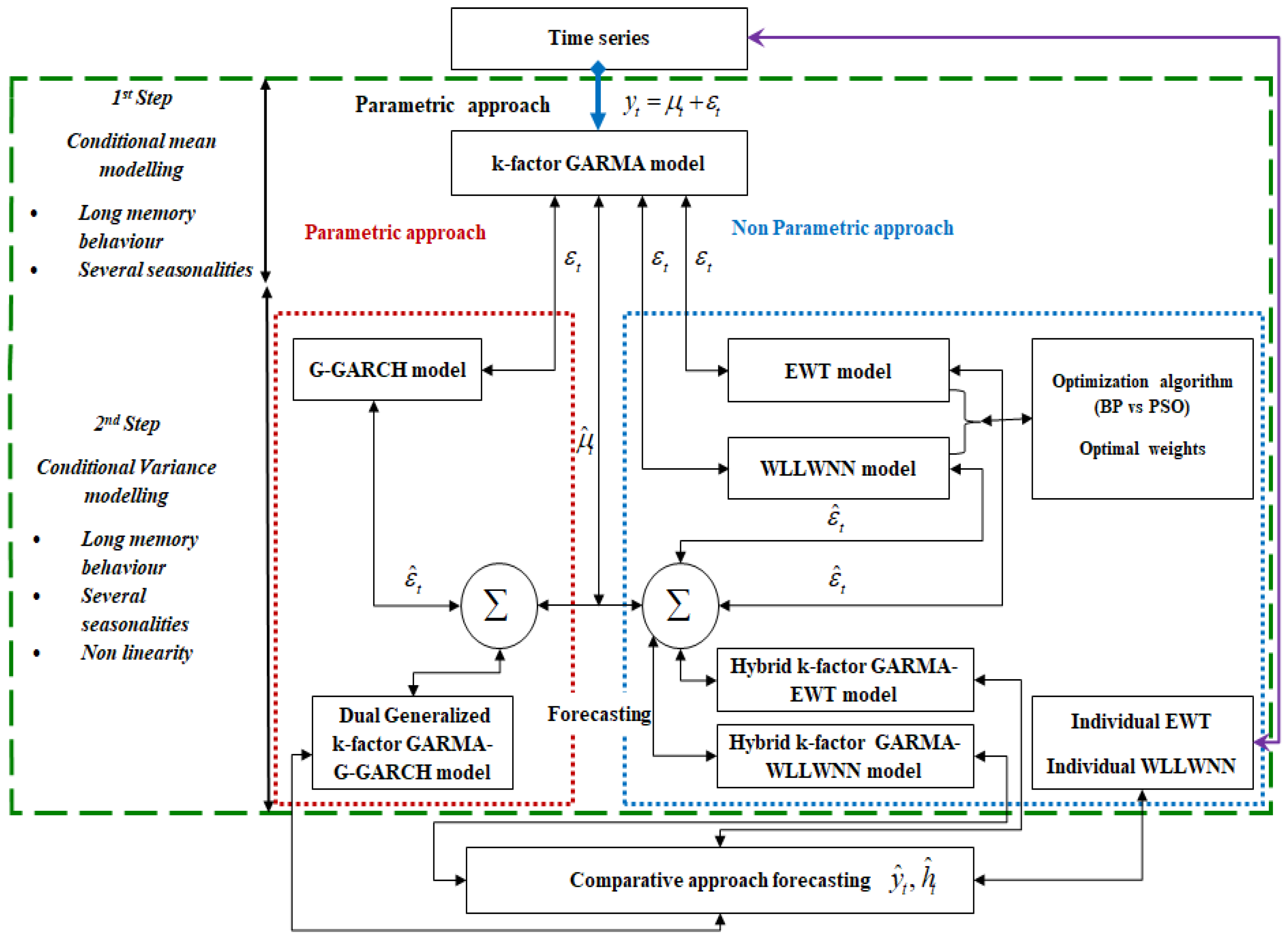
3. Econometric Methodology

3.1. The k-Factor GARMA Model

Gray et al. (1989) suggested a $k$-frequency GARMA model to generalize the ARFIMA model, permitting periodic or quasi-periodic movement in the signal, which is presented as

$$\Phi \left(B\right){\displaystyle \prod _{i=1}^k{\left(I-2{\nu }_{m,i}B+B^2\right)}^{d_{m,i}}\left(y_t-\mu \right)=\Theta \left(B\right){\epsilon }_t}$$

(1)

where $\Phi \left(B\right)$ and $\Theta \left(B\right)$ are the polynomials of the backshift operator $B$ such that all the roots of $\Phi \left(z\right)$ and $\Theta \left(z\right)$ lie outside the unit circle. The parameters ${\nu }_{m,i}$ offer information about periodic movement in the conditional mean, ${\epsilon }_t$ is a white noise disturbance sequence with variance ${\sigma }_{\epsilon }^2$, $k$ is a finite integer, $\left|{\nu }_{m,i}\right|<1$, $i=1, 2, \dots ,k$, $d_{m,i}$ are long-memory parameters of the conditional mean indicating how slowly the autocorrelations are damped, $\mu$ is the mean of the process, ${\lambda }_{m,i}={\cos }^{-1}({\nu }_{m,i})$, $i=1, 2, \dots ,k$, denote the Gegenbauer frequencies (G-frequencies). The GARMA model with $k$-frequency is stationary when $\left|{\nu }_{m,i}\right|<1$ and $d_{m,i}<1/2$ or when $\left|{\nu }_{m,i}\right|=1$ and $d_{m,i}<1/4$; the model exhibits a long memory when $d_{m,i}>0$. However, when it comes to a single frequency $\nu =1,$ the process is an ARFIMA $(p,d,q)$ model, and when $\nu =1$ and $d=1/2$, the process is an ARIMA model. Finally, when $d=0$, we acquire a stationary ARMA model. Cheung (1993) defines the spectral density function and displays that for $d>0$ the spectral density function has a pole at $\lambda ={\cos }^{-1}(\nu )$, which differs in the interval $\left[0,\pi \right]$. It is important to note that when $\left|\nu \right|<1$, the spectral density function is bounded at the origin for GARMA processes and thus does not suffer from many problems related with ARFIMA models (for more details, see Boubaker and Boutahar 2011; Boubaker 2015).

3.2. The Wavelet Local Linear Wavelet Neural Network

The wavelet local linear wavelet neural network (WLLWNN) involves the following. Initially, the historical data have been decomposed into wavelet-domain constitutive subseries using wavelet area and then using the local linear wavelet neural network (LLWNN) to form the WLLWNN forecasting model. The reader should consult Ben Amor et al. (2018) and Boubaker et al. (2020) for further details.

3.2.1. Theoretical Concepts of Wavelet

Wavelet decompositions are a useful tool in producing better local representation of the series in both frequency and time domain (Nicolaisen et al. 2000; Boubaker 2015, 2016). Wavelets are orthonormal bases attained through dyadically dilating and translating a pair of specially constructed functions denoted by $\phi$ and $\psi$, which are father wavelet (detected the smooth and low-frequency part of the time series) and mother wavelet (defined the detail and the high-frequency components), respectively, given by

$${\displaystyle \int \varphi (t)dt=1}\mathrm{and}{\displaystyle \int \psi (t)dt=0.}$$

(2)

The obtained wavelet basis is ${\varphi }_{j,k}\left(t\right)=2^{j/2}\varphi \left(2^{j}t-k\right)$ and ${\psi }_{j,k}\left(t\right)=2^{j/2}\psi \left(2^{j}t-k\right)$, where $j=1, \dots ,J$ indexes the scale and $k=1, \dots ,2^j$ indexes the translation. The parameter $j$ is adopted as the dilation parameter of the wave’s functions. This parameter $j$ adjusts the support of ${\psi }_{j,k}\left(t\right)$ to locally detect the features of high or low frequencies. The parameter $k$ is used to relocate the wavelets in the temporal scale. The number of observations limits the maximum number of scales that can be employed in the analysis $\left(T\ge 2^J\right)$. The localization property is a special property of the wavelet expansion, where the coefficient of ${\psi }_{j,k}\left(t\right)$ reveals information content of the function at approximate location $k{2}^{-j}$ and frequency $2^{-j}$. According to wavelets, all functions in $L^2(·)$ can be extended over the wavelet basis, exceptionally, as a linear combination at arbitrary level $J_0\in \mathbb{N}$ through different scales of the type

$$f\left(t\right)={\displaystyle \sum _k{s}_{J_0,k}}{\varphi }_{J_0,k}\left(t\right)+{\displaystyle \sum _{j\ge J}{\displaystyle \sum _k{d}_{j,k}{\psi }_{j,k}\left(t\right)}}$$

(3)

where ${\phi }_{J_0,k}$ is a scaling function with the corresponding coarse scale coefficients $s_{J_0,k}$ and $d_{j,k}$ are the detail coefficients, which measures the contribution of the corresponding wavelet to the function and constitutes the wavelet multiresolution analysis (MRA), given, respectively, by

$$s_{J_0,k}={\displaystyle \int f\left(t\right){\varphi }_{J_0,k}\left(t\right)dt}\mathrm{and}{d}_{j,k}={\displaystyle \int f\left(t\right){\psi }_{j,k}\left(t\right)dt}$$

(4)

In the following, the coefficients of the discrete wavelet transform can be deemed from the recursive MRA scheme, which is implemented by a two-channel filter bank illustration of the wavelet transform (i.e., a high-pass wavelet filter $\left\{h_l,l=0,\dots ,L-1\right\}$ and its associated low-pass scaling filter $\left\{g_l,l=0,\dots ,L-1\right\}$, satisfying the quadrature mirror relationship given by $g_l={\left(-1\right)}^{l+1}{h}_{L-1-l}$ for $l=0,\dots ,L-1$, where $L\in \mathbb{N}$ is the length of the filter). Moreover, Daubechies (1992) has constructed a class of wavelet functions which forms an orthonormal basis that possesses the smallest support of a given number of vanishing moments (the extremal phase filters $D\left(L\right)$ and the least asymmetric filters $La\left(L\right)$).

3.2.2. Empirical Wavelet Transforms

Conventional data pre-processing methods such as wavelet alter and Fourier convert approaches have some shortcomings, for example, the difficulty in choosing the mother wavelet. Similarly, empirical mode decomposition (EMD) which began with Hilbert–Huang transform (HHT) and was advanced by Huang et al. (1998), variational mode decomposition (VMD) by Dragomiretskiy and Zosso (2014) and ensemble empirical mode decomposition (EEMD) developed by Wu and Huang (2009) also have some disadvantages. In contrast, empirical wavelet transforms (EWT) were suggested by Gilles (2013) as a new adaptive time-frequency analysis method, taking into account the advantage of the empirical mode decomposition method and traditional wavelet analysis in signal processing. In the frequency-domain analysis of the signal, the Fourier spectrum is adaptively segmented by capturing the frequency-domain maximum point, and finally, the separation of different modes in the signal frequency component is realized. Indeed, the EWT is used as a processing tool to decompose the series into specific modal components according to the features of the signal. The main idea of EWT is based on the divided Fourier spectrum.

Note that the Fourier support interval $\left[0,\pi \right]$ is split into $N$ consecutive parts and ${\omega }_n$ represents the boundary between each segment with ${\lambda }_0=0$ and ${\lambda }_n=\pi$, and every pass filter can be defined as ${\Lambda }_n=\left[{\lambda }_{n-1},{\lambda }_n\right]$ and ${\displaystyle \underset{n=1}{\overset{N}{\cup }}{\Lambda }_n}=\left[0,\pi \right],$ $\forall n>0$. Following Cheng et al. (2019), the empirical wavelet’s function ${\widehat{\psi }}_n\left(\lambda \right)$ and the empirical scaling function ${\widehat{\varphi }}_n\left(\lambda \right)$ are given by the following formula:

$$\begin{array}{l}{\widehat{\psi }}_n\left(\lambda \right)=\{\begin{array}{l}1if {\lambda }_n+{\tau }_n\le \left|\lambda \right|<{\lambda }_{n+1}-{\tau }_{n+1}\\ cos\left[\frac{\pi }{2}\beta \left(\frac{1}{2{\tau }_n}\left(\left|\lambda \right|-{\lambda }_{n+1}+{\tau }_{n+1}\right)\right)\right]if {\lambda }_{n+1}-{\tau }_{n+1}\le \left|\lambda \right|<{\lambda }_{n+1}+{\tau }_{n+1}\\ sin\left[\frac{\pi }{2}\beta \left(\frac{1}{2{\tau }_n}\left(\left|\lambda \right|-{\lambda }_n+{\tau }_n\right)\right)\right]if {\lambda }_n-{\tau }_n\le \left|\lambda \right|<{\lambda }_n+{\tau }_n\\ \\ 0\mathrm{otherwise}\end{array}.\\ \mathrm{and}\\ {\widehat{\varphi }}_n\left(\lambda \right)=\{\begin{array}{l}1if \left|\lambda \right|<{\lambda }_n-{\tau }_n\\ cos\left[\frac{\pi }{2}\beta \left(\frac{1}{2{\tau }_n}\left(\left|\lambda \right|-{\lambda }_n+{\tau }_n\right)\right)\right]\\ 0\mathrm{otherwise}\end{array}if {\lambda }_n-{\tau }_n<\left|\lambda \right|<{\lambda }_n+{\tau }_n,\end{array}$$

(5)

where the proportional relationship between ${\tau }_n$ and ${\lambda }_n$ is ${\tau }_n=\gamma {\lambda }_n,0<\gamma <1$ and $\beta \left(x\right)$ satisfy $\beta \left(x\right)=\{\begin{array}{l}0,\forall x\le 0\\ 1,\forall x>1\end{array}$ along with $\beta \left(x\right)+\beta \left(1-x\right)=1, \forall x\in \left[0,1\right]$. The set $\left\{{\varphi }_1\left(t\right),{\left\{{\psi }_n\left(t\right)\right\}}_{n=1}^N\right\}$ is a tight frame of $L^2(\cdot )$. Thus, the EWT can be implemented in the same way as the classic wavelet transform, and the corresponding mathematical expression is as follows:

$$W_f^{\epsilon }\left(n, t\right)= \langle f\left(t\right),\psi \left(n, t\right)\rangle ={\displaystyle \int f\left(\tau \right)\overline{{\psi }_n\left(t-\tau \right)}d}\tau =F^{-1}\left(\widehat{f}\left(\omega \right),\overline{{\widehat{\psi }}_n\left(\omega \right)}\right).$$

(6)

where $W_f^{\epsilon }\left(n, t\right)$ is different frequency component of the empirical wavelet, and $F^{-1}(·)$ is the inverse Fourier transformation.

Ultimately, we can reconstruct the original signal as

$$\begin{array}{cc}\hfill f\left(t\right)& =W_f^{\epsilon }\left(0,t\right)\ast {\varphi }_1\left(t\right)+{\displaystyle \sum _{n=1}^N{W}_f^{\epsilon }\left(n,t\right)\ast {\psi }_n\left(t\right)}\hfill \\ & =F^{-1}\left({\widehat{W}}_f^{\epsilon }\left(0,\omega \right)\ast {\widehat{\varphi }}_1\left(\omega \right)+{\displaystyle \sum _{n=1}^N{\widehat{W}}_f^{\epsilon }\left(n,\omega \right)\ast {\widehat{\psi }}_n\left(\omega \right)}\right) \hfill \end{array}$$

(7)

where ${\widehat{W}}_f^{\epsilon }\left(0,\omega \right)$ and ${\widehat{W}}_f^{\epsilon }\left(n,\omega \right)$ are, respectively, the Fourier transformations of $W_f^{\epsilon }\left(0,t\right)$ and $W_f^{\epsilon }\left(n,t\right)$; $\ast$ is convolution symbol. Therefore, the empirical wavelet decomposition is expressed by $f_0\left(t\right)=W_f^{\epsilon }\left(0,t\right)\ast {\varphi }_1\left(t\right)$ and $f_k\left(t\right)=W_f^{\epsilon }\left(k,t\right)\ast {\varphi }_k\left(t\right)$. So, any series $f\left(t\right)$ can be defined as intrinsic mode function as $f\left(t\right)={\displaystyle \sum _{k=0}^N{f}_k\left(t\right)}$.

3.2.3. The Local Linear Wavelet Neural Network

The local linear wavelet neural network (LLWNN) of time-series forecasting was proposed by Chen et al. (2004) who proved that this modelization has more accuracy than the classic WNN. The LLWNN includes an input layer, hidden layer and linear output layer. In this case, the input series in the input layer of the network are diffused straight into the wavelet layer. The hidden layer neurons make use of wavelets as activation functions; these neurons are habitually called ‘wavelons’ (see Ben Amor et al. 2018 for more details about the method). As an alternative to exploiting multilayered neural networks and several variants, a WLLWNN is used for forecasting data. Regarding wavelet transformation theory, wavelets in the following form are a family of functions, produced from one single function $\psi \left(x\right)$ by the operation of dilation and translation.

$$\psi (x)=\left\{{\psi }_i={\left|a_i\right|}^{-1/2}\psi \left(\frac{x-b_i}{a_i}\right);a_i, b_i\in {ℝ}^n, i\in \mathbb{Z}\right\}$$

(8)

$x=\left(x_1, x_2, \dots , x_n\right)$,

$a_i=\left(a_{i1}, a_{i2}, \dots ,a_{in}\right)$,

$b_i=\left(b_{i1}, b_{i2}, \dots , b_{in} \right)$.

$\psi (x)$ is localized in both time space and the frequency space, called a mother wavelet, and the parameters $a_i$ and $b_i$ are the scale and translation parameters, respectively. Instead of the straightforward weight $w_i$ (piecewise constant model), a linear model $v_i=w_{i0}+w_{i1}{x}_1+\dots +w_{in}{x}_n$ is introduced.

The activities of the linear models $v_i$ $\left(i=1, \dots , n\right)$ are resolved by the associated locally active wavelet functions ${\psi }_i(x)$ $\left(i=1, \dots , n\right)$; thus, $v_i$ is the single significant variable. Nonlinear wavelet basis functions (named wavelets) are contained equally in time space and frequency space. Here, $m=n$ and output $\left(Y\right)$ of the suggested model is considered as

$$Y={\displaystyle \sum _{i=1}^M\left(w_{i0}+w_{i1}{x}_1+\dots +w_{in}{x}_n\right)}{\psi }_i\left(x\right)$$

(9)

The mother wavelet is

$$\psi (x)=\frac{-x^2}{2}{e}^{\frac{-x^2}{{\sigma }^2}}$$

(10)

$$\psi (x)=e^{-\left(\frac{x-c}{\sigma }\right)}{}^2$$

(11)

where

$$x=\sqrt{d_1^2+d_2^2+\dots +d_n^2}$$

(12)

To optimize the neural networks, the widely used learning algorithm is the back propagation (BP). Firstly, the parameters are randomly prepared, and after the algorithm measures the error between the output value and the real value, it lastly adjusts the weights in the direction of descendent gradient. The equations of the BP algorithm are offered in Burton and Harley (1994).

Moreover, Kennedy and Eberhart (1995) established the PSO as an optimization technique. In accord with other learning algorithms, the PSO clearly showed its efficacy. PSO algorithm is made through simulation of bird flocking in two-dimensional space. The position of each agent is denoted by $XY$-axis position, and the velocity is represented by $vx$ and $vy$. The agent position’s adjustment is documented by the location and the velocity information. The bird flocking optimizes the objective function. Each agent identifies its best value so far $\left(pbest\right)$ and its $XY$ place. In addition, each agent identifies the top value so far in the group $\left(gbest\right)$ between $\left(pbest\right)$. Mostly, each agent attempts to regulate its position using the following information:

(a) The distance between current position and $pbest$.

(b) The distance between the current position and $gbest$.

Velocity of each agent can be updated by the following equation:

$$v_i^{p+1}=w{v}_i^p+c_{1}ran{d}_1\times (pbes{t}_1-s_i^p)+c_{2}ran{d}_2(gbest-s_i^p)$$

(13)

where $v_i^p$ is the velocity of agent $i$ at iteration $p$, $w$ is the weight function, $c_j$ is weighting factor, $s_i^p$ is the current position of agent $i$ at iteration $p$, $pbes{t}_i$ is the $pbest$ of agent $i$ and $gbest$ is the $gbest$ of the group.

The velocity, which progressively gets closer to $pbest$ and $gbest$ can be computed using the above equation. The actual position, which characterizes the searching point in the solution space, can be updated using the following equation:

$$s_i^{p+1}=s^p+v_i^{p+1}$$

(14)

The PSO algorithm escapes from convergence toward a local minimum, because it is not based on gradient information contrary to the BP case (Abbass et al. 2001; Boubaker et al. 2020). The objective of the PSO is to produce the best set of weights (particle position) where numerous particles are moving to obtain the best solution, where the total number of weights characterizes the dimension of the search space. The optimization is finished when the personal best solution of each particle and the global best amount of the entire swarm are attained.

3.3. The Hybrid k-Factor GARMA-WLLWNN Model

Our hybrid approach combines a semi-parametric $k$-factor GARMA model and the proposed WLLWNN model. The $k$-factor GARMA model offers better flexibility in modeling simultaneous short- and long-term behavior of a seasonal time series. In addition, the selection of WLLWNN in our hybrid model is encouraged by the wavelet decomposition and its local linear modeling ability. It may be useful to think of time series as having two components: The first is a parametric form with unknown parameters, for which a parametric technique appears suitable. The residuals are the second component; this section normally has no special procedure. As a result, determining the right model to deal with this component of the time series is problematic. As a result, a nonparametric model appears to be the best choice for modeling the residuals. This choice is based on the notion that nonparametric models can decrease modeling bias by enforcing no specific model structure rather than a smoothness assumption and are thus particularly useful when we have little data or wish to be flexible with the underpinning model.

We consider a two-step approach; in the first stage, the purpose is modeling the conditional mean using a semi-parametric $k$-factor GARMA model. Conversely, residuals are important in forecasting time series; they may contain some information that is able to develop forecasting performance. Thus, in the second phase, the residuals resulting from the first step will be treated according to a novel wavelet local linear wavelet neural network (WLLWNN) model.

Hence, a time series can be written as

$$y_t={\mu }_t+{\epsilon }_t$$

(15)

where ${\mu }_t$ denotes the conditional mean of the time series, and ${\epsilon }_t$ is the residuals. In the head stage, the key purpose is the parametric modeling; therefore, the $k$-factor GARMA model is used to replicate the conditional mean (Equation (1)).

In the next stage, the residuals from the parametric model are used as a proxy for the corresponding volatility and modeled using the WLLWNN model. Let ${\epsilon }_t$ denote the residuals at time $t$ from the $k$-factor GARMA model, and then

$${\epsilon }_t=y_t-{\widehat{\mu }}_t$$

(16)

The first stage’s results are the forecast values and residuals of the semi-parametric modeling. In the following stage, the target is the modeling of the residuals using the WLLWNN with $n$ input nodes, and the WLLWNN for the residuals is

$${\epsilon }_t=f\left({\epsilon }_{t-1}, {\epsilon }_{t-2},\dots {\epsilon }_{t-n}\right)$$

(17)

where each ${\epsilon }_{t-i}$ is decomposed using the wavelet transform (Equation (3)), $f$ is a nonlinear, nonparametric function determined by the neural network with the reference to the current state of the data, during the training of the neural network. The output layer of the network (Equation (9)) gives the forecasting results.

$${\widehat{y}}_t={\widehat{\mu }}_t+{\widehat{\epsilon }}_t$$

(18)

As a consequence, this global prediction is the outcome of anticipating the time series’ conditional mean and conditional variance.

3.4. The k-Factor GARMA-G-GARCH Model

The conditional variance is assumed to be constant throughout time in the $k$-frequency GARMA model. Many time series are known to display volatility clustering, where time series have both high and low periods of volatility, according to empirical investigations. To duplicate these patterns, we added a fractional filter to the conditional variance equation of the $k$-factor GARMA model described above. As a result, we present the dual generalized $k$-factor GARMA-G-GARCH model, which can incorporate seasonality and long-memory dependency in the conditional mean and variance. The basic concept behind this model is to incorporate the generalized long-memory process into the GARCH equation that describes the evolution of conditional variance. This is why this new model category is known as Gegenbauer-GARCH (G-GARCH). To account for the presence of a time-varying conditional variance, we investigate the following $k$-factor GARMA process with G-GARCH-type innovations.

$$y_t={\mu }_t+{\epsilon }_t={\mu }_t+{\sigma }_t{z}_t$$

(19)

where ${\mu }_t$ is the conditional mean of $y_t$ modeling using the following $k$-factor GARMA process

$$\Phi \left(B\right){\displaystyle \prod _{i=1}^k{\left(I-2{\nu }_{m,i}B+B^2\right)}^{d_{m,i}}\left(y_t-\mu \right)=\Theta \left(B\right){\epsilon }_t}$$

(20)

$${\epsilon }_t/I_{t-1}\sim D\left(0,{\sigma }_t^2\right)$$

(21)

where ${\sigma }_t^2$ is the conditional variance, $I_{t-1}$ is the information up to time $t-1$, $z_t$ is a $i.i.d$ random variable with zero mean and unitary variance and $D(\cdot )$ is a probability density function. To define the conditional variance’s dynamics, the starting point is the dynamics of ${\epsilon }_t^2$. We assume that ${\epsilon }_t^2$ follow a $k$-factor GARMA model, which describes a cyclical pattern of length $S$.

$$\begin{array}{r}\left[{\left(I-B\right)}^{d_{v0}}{\left(I+B\right)}^{d_{v,k}I(E)}{\displaystyle \prod _{i=1}^{k-1}{\left(I-2{\nu }_{v,i}B+B^2\right)}^{d_{v,i}}}\right]\alpha \left(B\right){\epsilon }_t^2=\gamma +\left[I-\beta \left(B\right)\right]{\vartheta }_t,\\ P_v\left(B\right)\alpha \left(B\right){\epsilon }_t^2=\gamma +\left[I-\beta \left(B\right)\right]{\vartheta }_t.\end{array}$$

(22)

where $\alpha \left(B\right)=1-{\displaystyle \sum _{i=1}^q{\alpha }_i{B}^i}$ and $\beta \left(B\right)=1-{\displaystyle \sum _{i=1}^p{\beta }_i{B}^i}$ are suitable polynomials in the lag operator $B$ and ${\vartheta }_t={\epsilon }_t^2-{\sigma }_t^2$ is a martingale difference, $d_{v,0}=d_v/2,$ $I(E)=1$ if $S$ is even and zero otherwise.

With this assumption, the corresponding GARCH-type dynamics for conditional variance are given by

$${\sigma }_t^2=\gamma +\beta \left(B\right){\sigma }_t^2+\left[I-\beta \left(B\right)-P_v\left(B\right)\alpha \left(B\right)\right]{\epsilon }_t^2$$

(23)

This indicates that in the G-GARCH framework, each frequency has been modeled by means of a specific long-memory parameter $d_{v,i}$ (differencing parameter of the conditional variance). When $d_{v,0}=d_{v,1}=\dots =d_{v,k}$, all the involved frequencies have equal degree of memory. Model (23) can deliver, in this case, most of the existing GARCH models. For instance, standard GARCH models (including seasonal GARCH (Bollerslev and Hodrick (1992)) can be obtained by putting $d_{v,i}=0,i=0, \dots , k$. Similarly, the FIGARCH model is equivalent to $S=1$ and $0<d_{v,0}<1$. It is worth noting that generalized long-memory filters can theoretically be applied to any GARCH structure category. However, because G-GARCH models are not always practical due to the limitations required for conditional variance positive, Bordignon et al. (2007) advocated modeling the conditional variance logarithm. As a result, applying the filter to a generalized log-GARCH model provides a viable computational solution. This entails starting with the phrase

$$P_v\left(B\right)\alpha \left(B\right)\left[\ln ({\epsilon }_t^2)-\tau \right]=\gamma +\left[I-\beta \left(B\right)\right]{\vartheta }_t$$

(24)

where $P_v\left(B\right)$ is the generalized long-memory filter introduced into a GARCH structure, ${\vartheta }_t=\ln \left({\epsilon }_t^2\right)-\tau -\ln \left({\sigma }_t^2\right)$ is a martingale difference and $\tau =E\left[\ln \left(z_t^2\right)\right]$. The expected $\tau$ value depends on the distribution of the idiosyncratic shock and ensures that ${\vartheta }_t$ is a martingale difference, given that $\ln \left({\epsilon }_t^2\right)=\ln \left({\sigma }_t^2\right)+\ln \left(\right)z_t^2$. Under the Gaussian assumption, $\tau =-1.27$. The expression for conditional variance implied by (23) is

$$\ln \left({\sigma }_t^2\right)=\gamma +\beta \left(B\right)\ln \left({\sigma }_t^2\right)+\left[I-\beta \left(B\right)-P_v\left(B\right)\alpha \left(B\right)\right]\left[\ln \left({\epsilon }_t^2\right)-\tau \right]$$

(25)

Because we are modeling $\ln ({\sigma }_t^2)$ instead of ${\sigma }_t^2$, there are no requirements for variance positivity limitations. Adopting EGARCH versions of our model is another way to get around the problem of parameter limitations. To sum up, the purpose of this research consists of modeling the different patterns in the electricity time series to provide the best forecasting methods. For this determination, we exploit a hybrid methodology based on combining the semi-parametric $k$-factor GARMA model with a novel neural network named the EWLLWNN model. The performances of the proposed hybrid $k$-factor GARMA-EWLLWNN model are evaluated using data from the Polish electricity markets and matched with the dual comprehensive long-memory $k$-factor GARMA-G-GARCH model and the individual (E)WLLWNN, in order to demonstrate the resilience of the hybrid model we have proposed. The flow-chart construction of the hybrid GARMA-EWLLWNN model appears in Figure 1.

4. Empirical Methodology

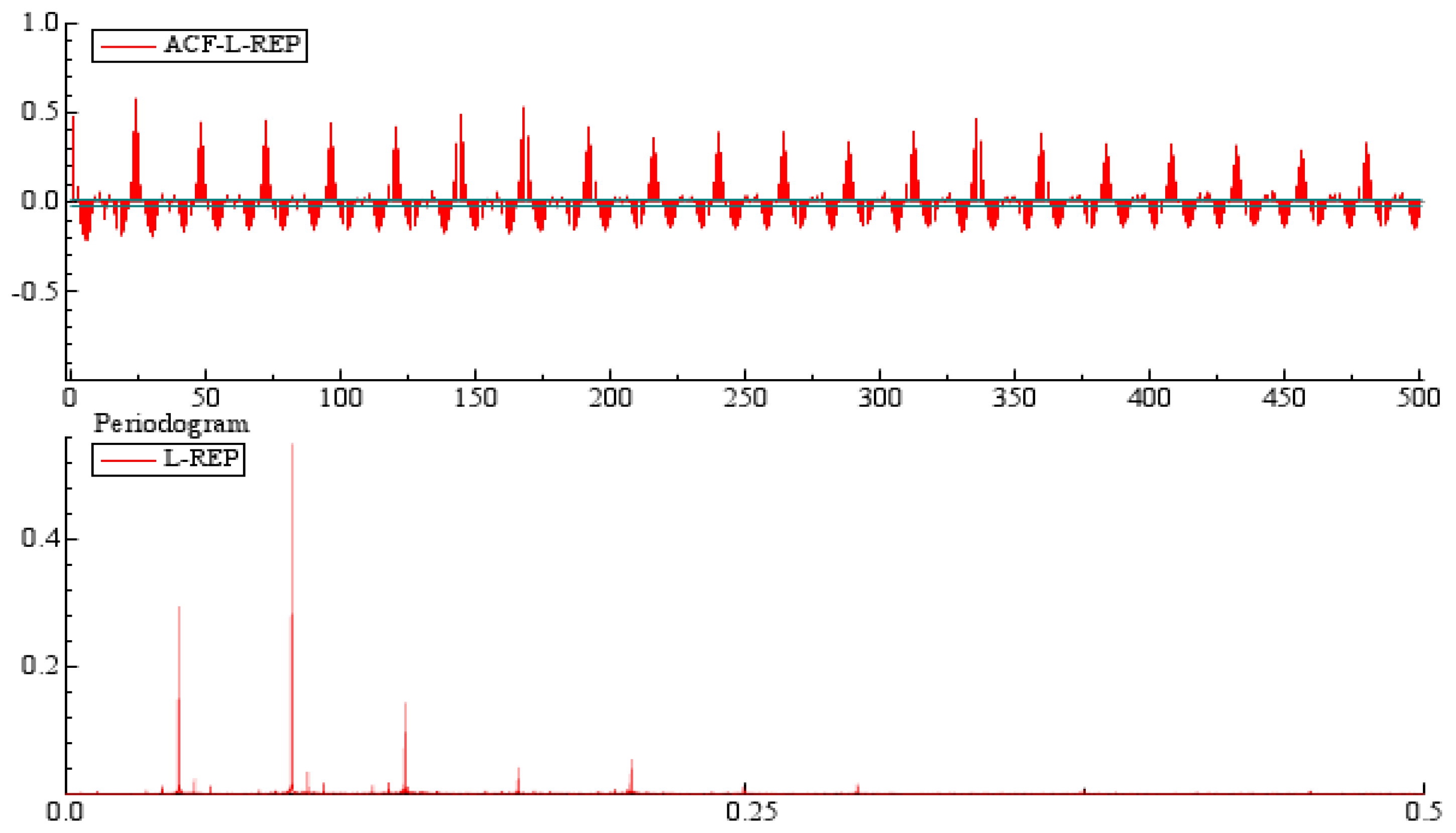
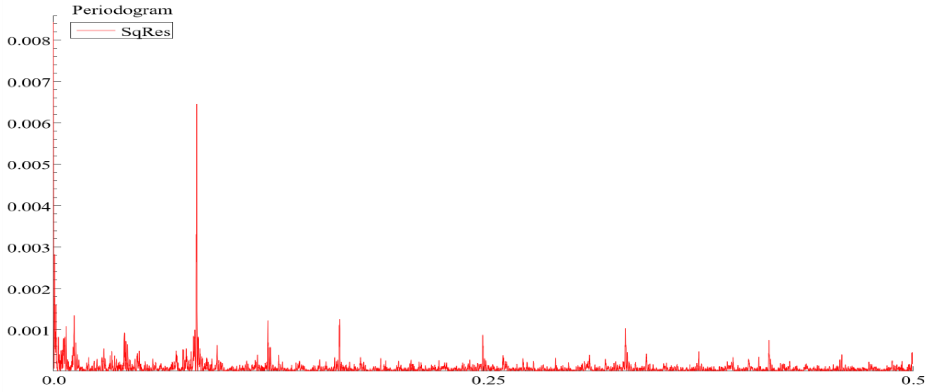
4.1. Data Description and Preliminary Study

After the liberalization of the electricity sector in 1999, the Polish power market was established, with electrical power being handled like any other commodity in a competitive market (instead the monopolistic market). The technique provided in this study is validated using hourly spot prices on the Polish power market between 10 January 2021 and 10 August 2022. Overall $T=5390$ hourly observations are shown in Figure 2. This information was taken from the Polish Power Exchange’s official website. We look at the logarithm of these series in this study because using the difference logarithm can make the series stationary and allow modeling of returns series ($R_t=\mathsf{\Delta }Log{P}_t$). As a result, we investigate the statistical and econometric characteristics of log-return electricity spot price series.

The log-return electricity price (abbreviated L-REP) shown in Figure 2 seem to fluctuate randomly around zero, while the variance varies over time with the alternation of volatile and tranquil periods. Moreover, L-REP series appears to have remained stable throughout time. Furthermore, the application of standard unit root tests and unit root tests show evidence of stationarity2. The return series illustrated in Figure 1 seem to fluctuate randomly around zero while the variance varies over time with alternation of volatile and tranquil periods.

Table 1. Descriptive statistics of the spot prices time series.

The Log-Returns Electricity Price
Mean	$-1.5478\times {10}^{-5}$
Standard Deviation	0.1079
Skewness	−0.2634
Excess Kurtosis	37.2358
Jarque–Bera	2.9826 × 105 ***

Note: *** denotes significance at 1% level.

shows the L-descriptive REP’s data in summary form. The standard deviation is low, indicating a non-symmetric distribution, whereas the series exhibit negative skewness and show excess kurtosis. Furthermore, the high kurtosis statistic indicates that the underlying data are leptokurtic. The observed asymmetry may indicate the presence of nonlinearities in the evolution process of returns. The departure from normality is confirmed by the Jarque–Bera test. Indeed, this test strongly rejects the null hypothesis of normality for the series, which means that minimum and maximum values deviate in higher number from the mean calculated. These findings clearly show that the probability of observing extremely negative and positive realizations for our return series is higher than that of a normal distribution.

As shown in Figure 3, for the log-return electricity price series (L-REP), the spectral density, traced by the periodogram, displays numerous peaks at equidistant frequencies, which demonstrates the presence of many seasonalities.

In addition, we use the GPH (Geweke and Porter-Hudak 1983) and local Whittle (LW) (Robinson 1995) semi-parametric techniques approach. For the GPH and LW tests, we need to choose a bandwidth, balancing a high variance caused by staying too close to the origin and using too little information and a bias induced by the contamination of the estimation through the short-memory component of the process. We apply three different bandwidths $T^{0.6}$, $T^{0.7}$ and $T^{0.8}$, where T is the sample size. The results of the GPH and LW tests do not prove to be sensitive to the choice of the bandwidth.

Table 2. Results of GPH and LW tests in the conditional mean.

L-REP	Bandwidth	GPH			LW
		${\widehat{d}}_m$	Standard error	p-value	${\widehat{d}}_m$	Standard error	p-value
	$T^{0.6}$ = 169	−0.51683	0.0558	0.0000	−0.5588	0.0403	0.0000
	$T^{0.7}$ = 397	−0.61336	0.0372	0.0000	−0.5775	0.0269	0.0000
	$T^{0.8}$ = 934	−0.4786	0.0253	0.0000	−0.5892	0.0178	0.0000

indicates that the log-return electricity price is stationary and mean reverting.

4.2. Estimation Results

4.2.1. The $k$-Factor GARMA Estimation Results

The seasonality can be detected without difficulty in the frequency domain ${\lambda }_i=1/T$, where $\lambda$ is the frequency of the seasonality and $T$ is the period of seasonality. As revealed, the spectral densities, denoted in the periodogram (see Figure 3), are unrestrained at equidistant frequencies, which demonstrates the existence of numerous seasonalities. The estimation results of the $k$-factor GARMA model, using the wavelets method, are reported in

Table 3. Estimation of the k-factor GARMA model: a wavelet-based approach.

Parameters	$\mathit{k}$-Factor GARMA Model Estimation
$\widehat{\mathsf{\Phi }}$	0.5132 ***
$\widehat{\mathsf{\Theta }}$	-
$\mu$	-
${\widehat{d}}_{m,1}$	0.1687 ***
${\widehat{d}}_{m,2}$	0.2349 ***
${\widehat{d}}_{m,3}$	0.4137 ***
${\widehat{\lambda }}_{m;1}$	0.0417 ***
${\widehat{\lambda }}_{m,2}$	0.0834 ***
${\widehat{\lambda }}_{m,3}$	0.1262 ***

Notes: *** denotes significance at 1% level.

. This result illustrates unusual peaks at frequencies ${\widehat{\lambda }}_{m;1}=0.0417$ ($T=23.9808$ $\approx$ 1 day), ${\widehat{\lambda }}_{m,2}=0.0834$ ($T=11.9904$ $\approx$ 1/2 day) and ${\widehat{\lambda }}_{m,3}=0.1262$ ($T=7.9239$ ≈ 1/3 day), corresponding to cycles with daily, semi-daily and third-daily periods, respectively. The results reveal that the $k$-factor GARMA adaptation appears to be the most satisfactory representation to describe the seasonal long-memory behavior of the L-REP series.

The next step consists of modeling the conditional variance, so the residuals of the $k$-factor GARMA estimation are formed using a new EWLLWNN as a first approach, and then addressed using the generalized GARCH model, known as G-GARCH, as a second approach, to determine the appropriate strategy.

4.2.2. The EWLLWNN Estimation Results

The residuals from the $k$-factor GARMA modeling are used as input for the innovative EWLLWNN and WLLWNN models to assess the conditional variance. All the inputs are normalized within a range of [0, 1] using the following formula before being applied to the network to eliminate the risk of coupling among distinct inputs and to accelerate convergence, which is regarded as the most generally used data smoothing approach: $y_{norm}=\frac{y_{org}-y_{\min }}{y_{\max }-y_{\min }}$, where $y_{norm}$ is the normalized value, $y_{org}$ is the original value and $y_{\min }$ and $y_{\max }$ are the minimum and maximum values of the corresponding residuals data, respectively. These normalized data are then decayed by means of the MODWT3 with Daubechies least asymmetric $\left(La\right)$ wavelet filter of length $L=8$ ($La(8)$). This wavelet filter has been recurrently assumed in the financial literature and it has been shown that $La\left(8\right)$ offers the greatest performance for the wavelet time-series decomposition. Our MODWT decomposition goes up to level $J=12$ which is specified by $J\le {\log }_2\left[\frac{T}{L-1}+1\right]$, i.e., where $T$ denotes the distance of the given time series and $L$ denotes the length of the filter (see Percival and Walden 2000; and Gençay et al. 2002). Indeed, our time series is decomposed into 12 components.

4.2.3. The LLWNN Modeling

The datasets are split into three parts: (a) a sample of 500 observations to start the network training, (b) a training set (4815 observations) and (c) a test set (72 observations). The forecasting experiment is carried out using an iterative forecasting method across the test set, with the model forecasting for 6, 12, 24, 48 and 72 h ahead. The parameters are randomly initialized at first to discover the optimum neural network design. The parameters are then modified using two separate algorithms: the back-propagation algorithm (BP) and the particle swarm optimization algorithm (PSO) to reduce the error between the output values and the real values throughout the network’s training.

4.2.4. The $k$-Factor GARMA-G-GARCH Estimation Results

The spectral distribution, Figure 4, traced by the periodogram, for the squared residuals of the $k$-factor GARMA model (the squared log-returns are used as a proxy for the associated volatility) exhibits numerous peaks at equidistant frequencies, proving the existence of various seasonalities. The findings of the GPH and LW demonstrate the existence of long memory in the conditional variance, as shown in

Table 4. Results of GPH and LW tests in the conditional variance.

L-REP	Bandwidth	GPH			LW
		${\widehat{d}}_v$	Standard error	p-value	${\widehat{d}}_v$	Standard error	p-value
	$T^{0.6}$ = 169	0.5275	0.0523	0.0000	0.4982	0.0381	0.0000
	$T^{0.7}$ = 397	0.3678	0.0329	0.0000	0.3874	0.0246	0.0000
	$T^{0.8}$ = 934	0.2379	0.0218	0.0000	0.2453	0.0249	0.0000

.

The G-GARCH model is used to evaluate the seasonal long-memory behavior in the conditional variance using the residuals from the $k$-factor GARMA. At equidistant frequencies, the spectral densities are unbounded, indicating the presence of multiple seasonality’s. The estimation results reported in

Table 5. The $k$-factor GARMA-G-GARCH estimation results.

$\mathit{k}$-Factor GARMA Model Estimation		The G-GARCH Model Estimation
$\widehat{\mathsf{\Phi }}$	0.6327 ***	$\widehat{\psi }$	0.7156 ***
$\widehat{\mathsf{\Theta }}$	-	$\widehat{\beta }$	0.5139 ***
$\mu$	-	$\widehat{\gamma }$	-
${\widehat{d}}_{m,1}$	0.1698 ***	${\widehat{d}}_{v,1}$	0.1497 ***
${\widehat{d}}_{m,2}$	0.2568 ***	${\widehat{d}}_{v,2}$	0.2678 ***
${\widehat{d}}_{m,3}$	0.3978 ***	${\widehat{d}}_{v,3}$	0.4319 ***
${\widehat{\lambda }}_{m,1}$	0.0405 ***	${\widehat{\lambda }}_{v,1}$	0.0411 ***
${\widehat{\lambda }}_{m,2}$	0.0838 ***	${\widehat{\lambda }}_{v,2}$	0.0854 ***
${\widehat{\lambda }}_{m,3}$	0.1289 ***	${\widehat{\lambda }}_{v,3}$	0.1197 ***

Notes: *** denotes significance at 1% level.

, indicating the long-range dependence in squared residuals of the GARMA process and strongly supporting the estimation of dynamic returns that allow for time-varying correlations. Moreover, the three different estimates of the long memory of the conditional variance are close to one another and less than 0.5, implying that the squared returns series is stationary and mean reverting, and long-memory processes require the use of some fractionally integrated method to estimate such processes.

The results of estimation of the k-factor GARMA-G-GARCH model are described in Table 5. They show special peaks at frequencies ${\widehat{\lambda }}_{v;1}=0.0411$ ($\approx$1 day), ${\widehat{\lambda }}_{v,2}=0.0854$ ($\approx$1/2 day) and ${\widehat{\lambda }}_{v,3}=0.1197$ ($\approx$1/3 day), which correspond to cycles with daily, semi-daily and third-daily periods, respectively.

4.3. Forecasting Results: A Comparative Approach

In a multi-step-ahead forecasting task, this section is devoted to evaluating the estimated models. We prefer to use out-of-sample criteria because predicting is essentially an out-of-sample problem. To ensure the accuracy and robustness of the modeling and forecasting findings, 5 distinct periods (6 h, 12 h, 1 day, 2 days and 3 days) were chosen. To assess the accuracy of the forecasting, we adopt two evaluation criteria, the mean absolute error ($MAE$) and the mean squared error ($MSE$), given, respectively, by $MAE=\frac{1}{N-t_1}{\displaystyle \sum _{t=t_1}^N\left|\left(y_{t+h}-{\widehat{y}}_{t,t+h}\right)\right|}$ and $MSE=\frac{1}{N-t_1}{\displaystyle \sum _{t=t_1}^N{\left(y_{t+h}-{\widehat{y}}_{t,t+h}\right)}^2}$, where $N$ is the number of observations, $N-t_1$ is the number of observations for predictive performance, $y_{t+h}$ is the log-return series through period $t+h$, ${\widehat{y}}_{t,t+h}$ is the predictive log-return series of the predictive horizon $h$ at time $t$.

To evaluate the suggested hybrid methodology’s prediction performance, the $k$-factor GARMA-WLLWNN was evaluated by two different models: the individual WLLWNN model and the $k$-factor GARMA-G-GARCH model. In terms of the network training, we used two alternative learning methods (BP and PSO). Furthermore, we used 5 time horizons for forecasting, 6 h, 12 h, 1 day, 2 days and 3 days ahead forecasting, using the $MAE$ and the $MSE$ out-of-sample criteria. Furthermore, we use Diebold and Mariano’s (1995) statistical test to conclude that the projections are equally accurate. The test statistics noted ($DM$) is asymptotically ${\rm N}\left(0, 1\right)$ distributed under the null hypothesis of no difference. However, the DM test requires the loss differential to be covariance stationary. Nevertheless, it may not be strictly necessary in some cases (Diebold 2015). In addition, the DM statistic can be obtained by regressing the loss differential on a constant, using Newey–West standard errors. To estimate the performance of the hybrid methodology forecast, we consider the $k$-factor GARMA-G-GARCH model for the purpose of comparison between the forecast results of all the other models. The significance level at 5% and 1% is displayed by ** and ***, respectively. Moreover, to better approve the predictive performances of our models, we use the model confidence set (MCS), introduced by Hansen et al. (2003), for the comparison of multiple forecast models at once. This model selection method is an innovative way to deal with the issue of selecting the best forecast model(s) using an out-of-sample evaluation under a specified loss function. In this work, we use the block bootstrap procedure and significance level $\alpha =5\%$ to determine the MCS p-values. The forecast models that are included in the 95% MCS are identified by an asterisk on the MSE. The forecast evaluation results are described in

Table 6. Out of sample forecasts results.

Models	Criterion	$h=6$	$h=12$		$h=24$
WLLWNN-based BP algorithm	$\mathrm{MAE}$	$6.3134\times {10}^{-5}$	$2.3486\times {10}^{-5}$		$7.5648\times {10}^{-5}$
	$\mathrm{MSE}$	$4.2321\times {10}^{-9}$	$2.2457\times {10}^{-10}$		$5.7365\times {10}^{-9}$
	$\mathrm{DM}$	1.1545	1.2874		1.3786
EWLLWNN-based BP algorithm	$\mathrm{MAE}$	$5.5623\times {10}^{-5}$	$1.5893\times {10}^{-5}$		$6.9873\times {10}^{-5}$
	$\mathrm{MSE}$	$3.4285\times {10}^{-9}$	$2.0445\times {10}^{-10}$		$4.8745\times {10}^{-9}$
	$\mathrm{DM}$	1.2334	1.2982		1.4684
WLLWNN-based PSO algorithm	$\mathrm{MAE}$	$2.3458\times {10}^{-7}$	$3.9523\times {10}^{-7}$		$10.2415\times {10}^{-7}$
	$\mathrm{MSE}$	$6.9982\times {10}^{-14}$	$2.2341\times {10}^{-13}$		$1.2134\times {10}^{-12}$
	$\mathrm{DM}$	1.3566	1.5562		1.6414
EWLLWNN-based PSO algorithm	$\mathrm{MAE}$	$2.2412\times {10}^{-7}$	$3.5932\times {10}^{-7}$		$9.9865\times {10}^{-7}$
	$\mathrm{MSE}$	$6.4532\times {10}^{-14}$	$2.0126\times {10}^{-13}$		$1.1625\times {10}^{-12}$
	$\mathrm{DM}$	1.3751	1.5875		1.7486
The hybrid $k$-factor GARMA-WLLWNN-based BP algorithm	$\mathrm{MAE}$	$4.4627\times {10}^{-5}$	$1.4341\times {10}^{-5}$		$6.6247\times {10}^{-5}$
	$\mathrm{MSE}$	$1.8653\times {10}^{-9}$	$1.8968\times {10}^{-10}$		$4.8791\times {10}^{-9}$
	$\mathrm{DM}$	1.9874 **	2.3536 **		2.7861 ***
The hybrid $k$-factor GARMA-EWLLWNN-based BP algorithm	$\mathrm{MAE}$	$4.2358\times {10}^{-5}$	$1.3652\times {10}^{-5}$		$6.1762\times {10}^{-5}$
	$\mathrm{MSE}$	$1.8342\times {10}^{-9}$	$1.7981\times {10}^{-10}$		$4.3871\times {10}^{-9}$
	$\mathrm{DM}$	2.0143 **	2.5462 **		2.8871 ***
The hybrid $k$-factor GARMA-WLLWNN-based PSO algorithm	$\mathrm{MAE}$	$1.4760\times {10}^{-9}$	$1.9674\times {10}^{-8}$		$3.4597\times {10}^{-9}$
	$\mathrm{MSE}$	$2.2175\times {10}^{-18}$	$5.3560\times {10}^{-16}$		$1.5261\times {10}^{-17}$
	$\mathrm{DM}$	2.6716 ***	2.9873 ***		3.5728 ***
The hybrid $k$-factor GARMA-EWLLWNN-based PSO algorithm	$\mathrm{MAE}$	$1.4372\times {10}^{-9}$	$1.9247\times {10}^{-8}$		$3.2655\times {10}^{-9}$
	$\mathrm{MSE}$	$2.0716\times {10}^{-18}$	$5.1038\times {10}^{-16}$		$1.4234\times {10}^{-17}$
	$\mathrm{DM}$	2.7861 ***	3.0837 ***		3.7981 ***
The $k$-factor GARMA-G-GARCH model	$\mathrm{MAE}$	$7.4882\times {10}^{-5}$	$7.8547\times {10}^{-5}$		$3.7866\times {10}^{-7}$
	$\mathrm{MSE}$	$4.5763\times {10}^{-14}$	$9.5376\times {10}^{-14}$		$1.8527\times {10}^{-15}$
Models	Criterion	$h=48$		$h=72$
WLLWNN-based BP algorithm	$\mathrm{MAE}$	$1.2834\times {10}^{-4}$		$3.4326\times {10}^{-4}$
	$\mathrm{MSE}$	$1.3543\times {10}^{-8}$		$7.3536\times {10}^{-8}$
	$\mathrm{DM}$	1.4932		1.6133
EWLLWNN-based BP algorithm	$\mathrm{MAE}$	$1.1382\times {10}^{-4}$		$2.9546\times {10}^{-4}$
	$\mathrm{MSE}$	$1.3312\times {10}^{-8}$		$6.8745\times {10}^{-8}$
	$\mathrm{DM}$	1.5623		1.7593
WLLWNN-based PSO algorithm	$\mathrm{MAE}$	$2.7863\times {10}^{-7}$		$3.9472\times {10}^{-7}$
	$\mathrm{MSE}$	$1.1568\times {10}^{-13}$		$2.2486\times {10}^{-13}$
	$\mathrm{DM}$	1.9645 **		2.2514 **
EWLLWNN-based PSO algorithm	$\mathrm{MAE}$	$2.5643\times {10}^{-7}$		$3.6765\times {10}^{-7}$
	$\mathrm{MSE}$	$1.1358\times {10}^{-13}$		$2.1378\times {10}^{-13}$
	$\mathrm{DM}$	20342 **		2.3436 **
The hybrid $k$-factor GARMA-WLLWNN-based BP algorithm	$\mathrm{MAE}$	$7.7763\times {10}^{-5}$		$8.9761\times {10}^{-5}$
	$\mathrm{MSE}$	$7.1321\times {10}^{-9}$		$9.1497\times {10}^{-9}$
	$\mathrm{DM}$	2.9784 ***		3.4836 ***
The hybrid $k$-factor GARMA-EWLLWNN-based BP algorithm	$\mathrm{MAE}$	$7.6408\times {10}^{-5}$		$8.4873\times {10}^{-5}$
	$\mathrm{MSE}$	$7.0265\times {10}^{-9}$		$8.9870\times {10}^{-9}$
	$\mathrm{DM}$	3.1426 ***		3.7625 ***
The hybrid $k$-factor GARMA-WLLWNN-based PSO algorithm	$\mathrm{MAE}$	$4.4379\times {10}^{-9}$		$2.4687\times {10}^{-8}$
	$\mathrm{MSE}$	$2.7859\times {10}^{-17}$		$7.5843\times {10}^{-16}$
	$\mathrm{DM}$	3.7633 ***		3.8921 ***
The hybrid $k$-factor GARMA-EWLLWNN-based PSO algorithm	$\mathrm{MAE}$	$4.2465\times {10}^{-9}$		$2.2274\times {10}^{-8}$
	$\mathrm{MSE}$	$2.7152\times {10}^{-17}$		$7.0872\times {10}^{-16}$
	$\mathrm{DM}$	3.9562 ***		4.1201 ***
The $k$-factor GARMA-G-GARCH model	$\mathrm{MAE}$	$4.6851\times {10}^{-8}$		$5.1257\times {10}^{-8}$
	$\mathrm{MSE}$	$2.3420\times {10}^{-15}$		$3.7871\times {10}^{-15}$

Notes: The significance level at 5% and 1% is displayed by ** and ***, respectively.

.

According to this table, it can be seen that the individual EWLLWNN-based PSO method outperforms the individual EWLLWNN-based BP algorithm, demonstrating the superiority of the PSO algorithm for neural network model training. This finding can be clarified by the fact that weights are updated in the direction of the negative gradient in BP algorithms. As a result, network training using BP methods has several disadvantages, such as sluggish convergence to a local minimum. Weights are branded by the particle position in the case of training with the PSO algorithm. The velocity and location of these particles are adjusted so as to find personal and global optimal values. This prevents the weights from converging to a local minimum.

Furthermore, the hybrid $k$-factor GARMA-EWLLWNN model outperforms all other computing approaches, as shown in Table 6. However, from this table, the ARFIMA-HY $k$-factor GARMA-EWLLWNN seems to be the only model included in the 95% MCS for all horizons under the MSE. In reality, this model combines the advantages of three techniques: first, the semi-parametric $k$-factor GARMA model, which detects and estimates both long memory and seasonality in the conditional mean; second, the empirical wavelet decomposition can produce a good local representation of the signal in both the time and frequency domains, making it a useful tool for revealing hidden patterns in electricity prices, such as high volatility, corrupted by occasional spikes, and followed by multiple seasonalities; and finally, the LLWNN model’s capability as a nonlinear, nonparametric model, as well as its uniqueness in having a wavelet activation function and local linearity, allows it to capture more nuanced characteristics of the data. As a consequence, the suggested hybrid $k$-factor GARMA-EWLLWNN is a robust tool that can handle the characteristics of power pricing while providing the best forecasting results. In sum, for all the evaluation criteria and forecast time horizons, the $k$-factor GARMA-EWLLWNN model prediction errors are the smallest.

5. Conclusions

In this research, we combine the parametric $k$-factor GARMA and the novel EWLLWNN models to produce a combined approach for electricity price forecasting. The $k$-factor GARMA model is used to evaluate the conditional mean of the time series because it can estimate the periodic long-memory behavior in the data. Second, the residuals from the $k$-factor GARMA model are utilized as a proxy for the associated volatility, and the empirical wavelet local linear neural network (EWLLWNN) model is used to estimate it. The data were divided into a wavelet-domain constitutional subseries and then injected into the network to construct the set of input variables in this network using empirical wavelet transform and form the proposed EWLLWNN forecasting model. On the other hand, while working with neural networks, it is critical to select the right training method; hence, this research compares two learning algorithms: the BP and PSO algorithms.

The projected hybrid model’s performance is assessed by means of data from the Polish electricity markets. To demonstrate the robustness of our suggested hybrid model, it is collated with the dual generalized long-memory $k$-factor GARMA-G-GARCH model and the individual (E) WLLWNN. The proposed $k$-factor GARMA-EWLLWNN approach is the best acceptable price forecasting strategy according to the empirical data. Because it produces fewer predicting errors than the other computing techniques, it is preferred. It could be considered a powerful forecasting method, especially when higher forecasting accuracy is required.

Related to other approaches, the innovation in our methodology lies in the combination of the seasonal long-memory estimation process, empirical wavelet decomposition and learning algorithms. Indeed, compared to other time-frequency analyses, the empirical wavelet method is used to improve the prediction accuracy of the artificial structure of the neural network. Moreover, we argue that this approach is a promising tool for modeling and forecasting the price of electricity.

In conclusion, the empirical example proved that the suggested hybrid algorithm can produce a superior predicting performance and that it is the best approach for forecasting the power market. Forecasts derived from benchmark datasets further demonstrate the usefulness of our technique in terms of reliability evaluation and prediction optimization. Finally, our results are of major interest to researchers, regulators and market participants. In fact, our findings may be valuable for energy market players, international asset allocation and risk management as a strategy for predicting power prices.

As a proposal for future work, we suggest comparing our hybrid approach to other artificial neural network algorithms as well as other recently used decomposition procedures in order to validate the stability of the prediction results obtained for different forecast horizons.

References

1. Abbass, Hussein A., Ruhul Sarker, and Charles Newton. 2001. A Pareto-frontier Differential Evolution Approach for Multi-objective Optimization Problems. IEEE Congress on Evolutionary Computation 2: 971–978. [Google Scholar]
2. Aggarwal, S. K., L. M. Saini, and Ashwani Kumar. 2008. Price Forecasting Using Wavelet Transform and LSE Based Mixed Model in Australian Electricity Market. International Journal of Energy Sector Management 2: 521–46. [Google Scholar] [CrossRef]
3. Anbazhagan, S., and N. Kumarappan. 2014. Day-Ahead Deregulated Electricity Market Price Forecasting Using Neural Network Input Featured by DCT. Energy Conversion and Management 78: 711–19. [Google Scholar] [CrossRef]
4. Armano, Giuliano, Michele Marchesi, and Andrea Murru. 2005. A Hybrid Genetic-Neural Architecture for Stock Indexes Forecasting. Information Sciences 170: 3–33. [Google Scholar] [CrossRef]
5. Athanassios, Kintsakis, Antonios Chrysopoulos, and Pericles A. Mitkas. 2015. Agent-based Short-Term Load and Price Forecasting Using a Parallel Implementation of an Adaptive PSO-Trained Local Linear Wavelet Neural Network. Paper presented at International Conference on the European Energy Market, Lisbon, Portugal, May 19–22. [Google Scholar]
6. Baillie, Richard T., Bollerslev Tim Mikkelsen, and Hans Ole Mikkelsen. 1996. Fractionally integrated generalized autoregressive conditional heteroskedasticity. Journal of Econometrics 74: 3–30. [Google Scholar] [CrossRef]
7. Bashir, Zidan, and M. E. El-Hawary. 2000. Short Term Load Forecasting by Using Wavelet Neural Networks. Paper presented at 2000 Canadian Conference on Electrical and Computer Engineering. Conference, Halifax, NS, Canada, May 7–10; vol. 1, pp. 163–66. [Google Scholar] [CrossRef]
8. Ben Amor, Souhir, Heni Boubaker, and Lotfi Belkacem. 2018. Forecasting Electricity Spot Price for Nord Pool Market with a Hybridk-Factor Garma-LLWNN Model. Journal of Forecasting 37: 832–51. [Google Scholar] [CrossRef]
9. Benaouda, D., F. Murtagh, J.-L. Starck, and O. Renaud. 2006. Wavelet-Based Nonlinear Multiscale Decomposition Model for Electricity Load Forecasting. Neurocomputing 70: 139–54. [Google Scholar] [CrossRef]
10. Beran, Jan. 1994. Statistics for Long Memory Processes. New York: Chapman & Hall. [Google Scholar]
11. Bollerslev, Tim. 1986. Generalized autoregressive conditional heteroskedasticity. Journal of Econometrics 31: 307–27. [Google Scholar] [CrossRef]
12. Bollerslev, Tim, and Hans Ole Mikkelsen. 1996. Modeling and Pricing Long Memory in Stock Market Volatility. Journal of Econometrics 73: 151–84. [Google Scholar] [CrossRef]
13. Bollerslev, Tim, and Robert Hodrick. 1992. Financial Market Efficiency Tests. Cambridge: National Bureau of Economic Research. [Google Scholar] [CrossRef]
14. Bordignon, Silvano, Massimiliano Caporin, and Francesco Lisi. 2007. Generalised Long-Memory GARCH Models for Intra-Daily Volatility. Computational Statistics & Data Analysis 51: 5900–12. [Google Scholar] [CrossRef]
15. Bordignon, Silvano, Massimiliano Caporin, and Francesco Lisi. 2008. Periodic Long-Memory GARCH Models. Econometric Reviews 28: 60–82. [Google Scholar] [CrossRef]
16. Boubaker, Heni, and Mohamed Boutahar. 2011. A Wavelet-Based Approach for Modelling Exchange Rates. Statistical Methods & Applications 20: 201–20. [Google Scholar] [CrossRef]
17. Boubaker, Heni, and Nadia Sghaier. 2015. Semiparametric Generalized Long-Memory Modeling of Some MENA Stock Market Returns: A Wavelet Approach. Economic Modelling 50: 254–65. [Google Scholar] [CrossRef]
18. Boubaker, Heni, Souhir Ben Amor, and Hichem Rezgui. 2020. A New Hybrid Wavelet-Neural Network Approach for Forecasting Electricity. Energy Studies Review 24. [Google Scholar] [CrossRef]
19. Boubaker, Heni. 2015. Wavelet Estimation of Gegenbauer Processes: Simulation and Empirical Application. Computational Economics 46: 551–74. [Google Scholar] [CrossRef]
20. Boubaker, Heni. 2016. A Comparative Study of the Performance of Estimating Long-Memory Parameter Using Wavelet-Based Entropies. Computational Economics 48: 693–731. [Google Scholar] [CrossRef]
21. Bunn, Derek W., and Nektaria Karakatsani. 2003. Modeling and Forecasting Electricity Prices. London: London Business School. [Google Scholar]
22. Burton, Bruce, and Ronald G. Harley. 1994. Reducing the computational demands of continually online trained artificial neural networks for system identification and control of fast processes. Paper presented at 1994 IEEE Industry Applications Society Annual Meeting, Denver, CO, USA, October 2–5; vol. 2, pp. 1836–43. [Google Scholar]
23. Cao, Liangyue, Yiguang Hong, Haiping Fang, and Guowei He. 1995. Predicting Chaotic Time Series with Wavelet Networks. Physica D: Nonlinear Phenomena 85: 225–38. [Google Scholar] [CrossRef]
24. Caporale, Guglielmo Maria, and Luis Gil-Alana. 2014. Long-Run and Cyclical Dynamics in the US Stock Market. Journal of Forecasting 33: 147–61. [Google Scholar] [CrossRef]
25. Caporin, Massimiliano, and Francesco Lisi. 2010. MISSPECIFICATION Tests for Periodic Long Memory GARCH Models. Statistical Methods and Applications 19: 47–62. [Google Scholar] [CrossRef]
26. Chakravarty, S., Maya Nayak, and R. Bisoi. 2012. Particle Swarm Optimization Based Local Linear Wavelet Neural Network for Forecasting Electricity Prices. Presented at 2012 International Conference on Energy, Automation and Signal, Bhubaneswar, India, December 28–30. [Google Scholar] [CrossRef]
27. Chen, Yuehui, Jiwei Dong, Bo Yang, and Yong Zhang. 2004. A local linear wavelet neural network. Paper presented at Fifth World Congress on Intelligent Control and Automation (IEEE Cat. No. 04EX788), Hangzhou, China, June 15–19; vol. 3, pp. 1954–57. [Google Scholar]
28. Cheng, Hangyang, Xiangwu Ding, Wuneng Zhou, and Renqiang Ding. 2019. A Hybrid Electricity Price Forecasting Model with Bayesian Optimization for German Energy Exchange. International Journal of Electrical Power & Energy Systems 110: 653–66. [Google Scholar] [CrossRef]
29. Cheung, Yin-Wong. 1993. Long Memory in Foreign-Exchange Rates. Journal of Business & Economic Statistics 11: 93–101. [Google Scholar] [CrossRef]
30. Contreras, Javier, Rosario Espinola, Fransicico J. Nogales, and Antonio J. Conejo. 2003. Arima Models to Predict next-Day Electricity Prices. IEEE Transactions on Power Systems 18: 1014–20. [Google Scholar] [CrossRef]
31. Cristea, Paul, Rodica Tuduce, and Alexandra Cristea. 2000. Time Series Prediction with Wavelet Neural Networks. Paper presented at 5th Seminar on Neural Network Applications in Electrical Engineering, NEUREL 2000 (IEEE Cat. No.00EX287), Belgrade, Yugoslavia, September 27. [Google Scholar]
32. Daubechies, Ingrid. 1992. Ten Lectures on Wavelets. Philadelphia: Society for Industrial and Applied Mathematics. [Google Scholar] [CrossRef]
33. Diebold, Francis X. 2015. Comparing Predictive Accuracy, Twenty Years Later: A Personal Perspective on the Use and Abuse of Diebold-Mariano Tests. Journal of Business and Economic Statistics 33: 1–9. [Google Scholar] [CrossRef]
34. Diebold, Francis X., and Roberto S. Mariano. 1995. Comparing Predictive Accuracy. Journal of Business & Economic Statistics 13: 253–63. [Google Scholar] [CrossRef]
35. Diongue, Abdou Kâ, Dominique Guégan, and Bertrand Vignal. 2009. Forecasting Electricity Spot Market Prices with a K-Factor GIGARCH Process. Applied Energy 86: 505–10. [Google Scholar] [CrossRef]
36. Dragomiretskiy, Konstantin, and Dominique Zosso. 2014. Variational Mode Decomposition. IEEE Transactions on Signal Processing 62: 531–44. [Google Scholar] [CrossRef]
37. Engle, Robert F. 1982. Autoregressive Conditional Heteroscedasticity with Estimates of the Variance of United Kingdom Inflation. Econometrica 50: 987. [Google Scholar] [CrossRef]
38. Escribano, Alvaro, J. Ignacio Peña, and Pablo Villaplana. 2011. Modelling Electricity Prices: International Evidence*. Oxford Bulletin of Economics and Statistics 73: 622–50. [Google Scholar] [CrossRef]
39. Gao, Rong, and Lefteri H. Tsoukalas. 2001. Neural-Wavelet Methodology for Load Forecasting. Journal of Intelligent and Robotic Systems 31: 149–57. [Google Scholar] [CrossRef]
40. Garcia, Reinaldo C., Javier Contreras, Macro van Akkeren, and João Batista C. Garcia. 2005. A GARCH Forecasting Model to Predict Day-Ahead Electricity Prices. IEEE Transactions on Power Systems 20: 867–74. [Google Scholar] [CrossRef]
41. Gençay, Ramazan, Faruk Selçuk, and Brandon Whitcher. 2002. An Introduction to Wavelets and Other Filtering Methods in Finance and Economics. Waltham. Cambridge: Academic Press, pp. 1–14. [Google Scholar] [CrossRef]
42. Geweke, John, and Susan Porter-Hudak. 1983. The Estimation and Application of Long Memory Time Series Models. Journal of Time Series Analysis 4: 221–38. [Google Scholar] [CrossRef]
43. Ghosh, Sajal, and Kakali Kanjilal. 2014. Modelling and Forecasting of Day-Ahead Electricity Price in Indian Energy Exchange—Evidence from MSARIMA-EGARCH Model. International Journal of Indian Culture and Business Management 8: 413. [Google Scholar] [CrossRef]
44. Gilles, Jerome. 2013. Empirical Wavelet Transform. IEEE Transactions on Signal Processing 61: 3999–4010. [Google Scholar] [CrossRef]
45. Girish, Godekere P. 2016. Spot Electricity Price Forecasting in Indian Electricity Market Using Autoregressive-GARCH Models. Energy Strategy Reviews 11–12: 52–57. [Google Scholar] [CrossRef]
46. Granger, Clive W. 1989. Invited Review Combining Forecasts—Twenty Years Later. Journal of Forecasting 8: 167–73. [Google Scholar] [CrossRef]
47. Granger, Clive W., and Roselyne Joyeux. 1980. An Introduction to Long-Memory Time Series Models and Fractional Differencing. Journal of Time Series Analysis 1: 15–29. [Google Scholar] [CrossRef]
48. Gray, Henry L., Nien-Fan Zhang, and Wayne A. Woodward. 1989. On Generalized Fractional Processes. Journal of Time Series Analysis 10: 233–57. [Google Scholar] [CrossRef]
49. Grossi, Luigi, and Fany Nan. 2019. Robust Forecasting of Electricity Prices: Simulations, Models and the Impact of Renewable Sources. Technological Forecasting and Social Change 141: 305–18. [Google Scholar] [CrossRef]
50. Hansen, Peter Reinhard, Asger Lunde, and James M. Nason. 2003. Choosing the best volatility models: The model confidence set approach. Oxford Bulletin of Economics and Statistics 65: 839–61. [Google Scholar] [CrossRef]
51. Hosking, J. R. 1981. Fractional Differencing. Biometrika 68: 165–76. [Google Scholar] [CrossRef]
52. Huang, Norden E., Zheng Shen, Steven R. Long, Manli C. Wu, Hsing H. Shih, Quanan Zheng, Nai-Chyuan Yen, Chi Chao Tung, and Henry H. Liu. 1998. The Empirical Mode Decomposition and the Hilbert Spectrum for Nonlinear and Non-Stationary Time Series Analysis. Proceedings of the Royal Society of London. Series A: Mathematical, Physical and Engineering Sciences 454: 903–95. [Google Scholar] [CrossRef]
53. Huisman, Ronald, Christian Huurman, and Ronald Mahieu. 2007. Hourly Electricity Prices in Day-Ahead Markets. Energy Economics 29: 240–48. [Google Scholar] [CrossRef]
54. Jabeur, Sami Ben, Salma Mefteh-Wali, and Jean-Laurent Viviani. 2021. Forecasting Gold Price with the XGBOOST Algorithm and Shap Interaction Values. Annals of Operations Research. [Google Scholar] [CrossRef]
55. Jiang, Manrui, Lifen Jia, Zhensong Chen, and Wei Chen. 2020. The Two-Stage Machine Learning Ensemble Models for Stock Price Prediction by Combining Mode Decomposition, Extreme Learning Machine and Improved Harmony Search Algorithm. Annals of Operations Research 309: 553–85. [Google Scholar] [CrossRef]
56. Jiang, Ping, Feng Liu, and Yiliao Song. 2017. A Hybrid Forecasting Model Based on Date-Framework Strategy and Improved Feature Selection Technology for Short-Term Load Forecasting. Energy 119: 694–709. [Google Scholar] [CrossRef]
57. Kennedy, James, and Russell Eberhart. 1995. Particle Swarm Optimization. Paper presented at Proceedings of ICNN’95—International Conference on Neural Networks, Perth, WA, Australia, November 27–December 1. [Google Scholar]
58. Khashei, Mehdi, and Mehdi Bijari. 2010. An Artificial Neural Network (p,D,Q) Model for Timeseries Forecasting. Expert Systems with Applications 37: 479–89. [Google Scholar] [CrossRef]
59. Knittel, Christopher R., and Michael R. Roberts. 2005. An Empirical Examination of Restructured Electricity Prices. Energy Economics 27: 791–817. [Google Scholar] [CrossRef]
60. Koopman, Siem Jan, Marius Ooms, and M. Angeles Carnero. 2007. Periodic Seasonal Reg-Arfima–GARCH Models for Daily Electricity Spot Prices. Journal of the American Statistical Association 102: 16–27. [Google Scholar] [CrossRef]
61. Liu, Heping, and Jing Shi. 2013. Applying Arma–GARCH Approaches to Forecasting Short-Term Electricity Prices. Energy Economics 37: 152–66. [Google Scholar] [CrossRef]
62. Mallat, Stéphane. 1999. A Wavelet Tour of Signal Processing. New York: Academic Press. [Google Scholar]
63. Mallat, Stéphane G., and Zhifeng Zhang. 1993. Matching Pursuits with Time-Frequency Dictionaries. IEEE Transactions on Signal Processing 41: 3397–3415. [Google Scholar] [CrossRef]
64. Nicolaisen, James D., C. W. Richter, and Gerald B. Sheble. 2000. Price Signal Analysis for Competitive Electric Generation Companies. Paper presented at DRPT2000. International Conference on Electric Utility Deregulation and Restructuring and Power Technologies. Proceedings (Cat. No.00EX382), London, UK, April 4–7. [Google Scholar]
65. Panapakidis, Ioannis P., and Athanasios S. Dagoumas. 2016. Day-ahead electricity price forecasting via the application of artificial neural network based models. Applied Energy 172: 132–51. [Google Scholar] [CrossRef]
66. Pany, Prasanta Kumar. 2011. Short-Term Load Forecasting Using PSO Based Local Linear Wavelet Neural Network. International Journal of Instrumentation Control and Automation 1: 163–68. [Google Scholar] [CrossRef]
67. Percival, Donald B., and Andrew T. Walden. 2000. Wavelet Methods for Time Seriesanalysis. Cambridge: Cambridge University Press. [Google Scholar] [CrossRef]
68. Rana, Mashud, and Irena Koprinska. 2016. Forecasting Electricity Load with Advanced Wavelet Neural Networks. Neurocomputing 182: 118–32. [Google Scholar] [CrossRef]
69. Robinson, P. M. 1995. Log-Periodogram Regression of Time Series with Long Range Dependence. The Annals of Statistics 23. [Google Scholar] [CrossRef]
70. Shafie-khah, M., M. Parsa Moghaddam, and M.K. Sheikh-El-Eslami. 2011. Price Forecasting of Day-Ahead Electricity Markets Using a Hybrid Forecast Method. Energy Conversion and Management 52: 2165–69. [Google Scholar] [CrossRef]
71. Sharkey, Amanda J. 2002. Types of Multinet System. In Multiple Classifier System. Berlin/Heidelberg: Springer, pp. 108–17. [Google Scholar] [CrossRef]
72. Soares, Lacir Jorge, and Leonardo Rocha Souza. 2006. Forecasting Electricity Demand Using Generalized Long Memory. International Journal of Forecasting 22: 17–28. [Google Scholar] [CrossRef]
73. Szkuta, Boguslaw R., L. Augusto Sanabria, and Tharam S. Dillon. 1999. Electricity Price Short-Term Forecasting Using Artificial Neural Networks. IEEE Transactions on Power Systems 14: 851–57. [Google Scholar] [CrossRef]
74. Tan, Zhongfu, Jinliang Zhang, Jianhui Wang, and Jun Xu. 2010. Day-Ahead Electricity Price Forecasting Using Wavelet Transform Combined with Arima and GARCH Models. Applied Energy 87: 3606–10. [Google Scholar] [CrossRef]
75. Tseng, Fang-Mei, Hsiao-Cheng Yu, and Gwo-Hsiung Tzeng. 2002. Combining Neural Network Model with Seasonal Time Series Arima Model. Technological Forecasting and Social Change 69: 71–87. [Google Scholar] [CrossRef]
76. Valenzuela, Olga, I. Rojas, F. Rojas, H. Pomares, L. J. Herrera, A. Guillen, L. Marquez, and M. Pasadas. 2008. Hybridization of Intelligent Techniques and ARIMA Models for Time Series Prediction. Fuzzy Sets and Systems 159: 821–45. [Google Scholar] [CrossRef]
77. Wang, A. J., and B. Ramsay. 1998. A Neural Network Based Estimator for Electricity Spot-Pricing with Particular Reference to Weekend and Public Holidays. Neurocomputing 23: 47–57. [Google Scholar] [CrossRef]
78. Weron, Rafał, Ingve Simonsen, and Piotr Wilman. 2004. Modeling Highly Volatile and Seasonal Markets: Evidence from the Nord Pool Electricity Market. In The Application of Econophysics. Tokyo: Springer, pp. 182–91. [Google Scholar] [CrossRef]
79. Whitcher, Brandon. 2004. Wavelet-Based Estimation for Seasonal Long-Memory Processes. Technometrics 46: 225–38. [Google Scholar] [CrossRef]
80. Woodward, Wayne A., Qin C. Cheng, and Henry L. Gray. 1998. A K-Factor Garma Long-Memory Model. Journal of Time Series Analysis 19: 485–504. [Google Scholar] [CrossRef]
81. Wu, Zhaohua, and Norden E. Huang. 2009. Ensemble Empirical Mode Decomposition: A Noise-Assisted Data Analysis Method. Advances in Adaptive Data Analysis 1: 1–41. [Google Scholar] [CrossRef]
82. Yao, S. J., Y. H. Song, L. Z. Zhang, and X. Y. Cheng. 2000. Wavelet Transform and Neural Networks for Short-Term Electrical Load Forecasting. Energy Conversion and Management 41: 1975–88. [Google Scholar] [CrossRef]
83. Yu, Lean, Shouyang Wang, and Kin Keung Lai. 2005. A Novel Nonlinear Ensemble Forecasting Model Incorporating GLAR and Ann for Foreign Exchange Rates. Computers & Operations Research 32: 2523–41. [Google Scholar] [CrossRef]
84. Zhang, G. Peter. 2003. Time Series Forecasting Using a Hybrid Arima and Neural Network Model. Neurocomputing 50: 159–75. [Google Scholar] [CrossRef]
85. Zhang, Jinliang, Yi-Ming Wei, Dezhi Li, Zhongfu Tan, and Jianhua Zhou. 2018. Short Term Electricity Load Forecasting Using a Hybrid Model. Energy 158: 774–81. [Google Scholar] [CrossRef]
86. Zhang, Qinghua, and Albert Benveniste. 1992. Wavelet Networks. IEEE Transactions on Neural Networks 3: 889–98. [Google Scholar] [CrossRef]
Figure 1. The implemented hybrid procedure.
Jrfm 16 00246 g001
Figure 2. Hourly log-return of spot price for Polish electricity market.
Jrfm 16 00246 g002
Figure 3. Polish L-REP ACF and Periodogram.
Jrfm 16 00246 g003
Figure 4. Periodogram of the squared residuals of the k -factor GARMA model.
Jrfm 16 00246 g004