
A New Nonlinear Dynamic Speed Controller for a Differential Drive Mobile Robot

 ,
, 

 , ,
, ,  and
and
Abstract
:1. Introduction
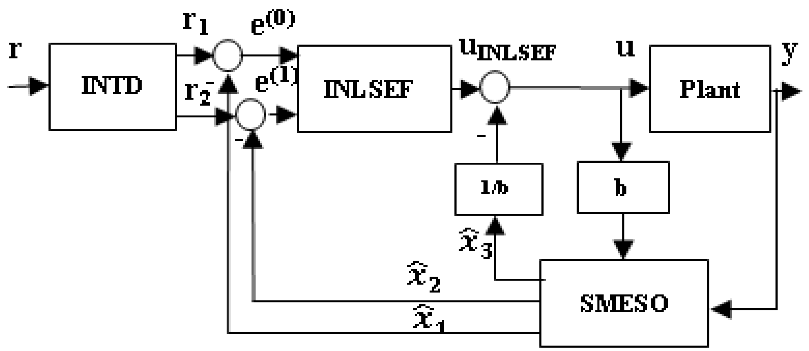
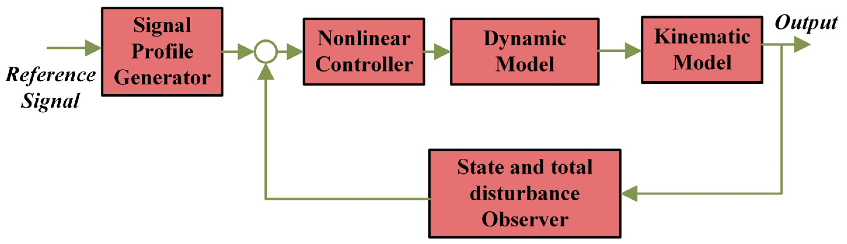
2. The Main Results: Improved Active Disturbance Rejection Control (IADRC)
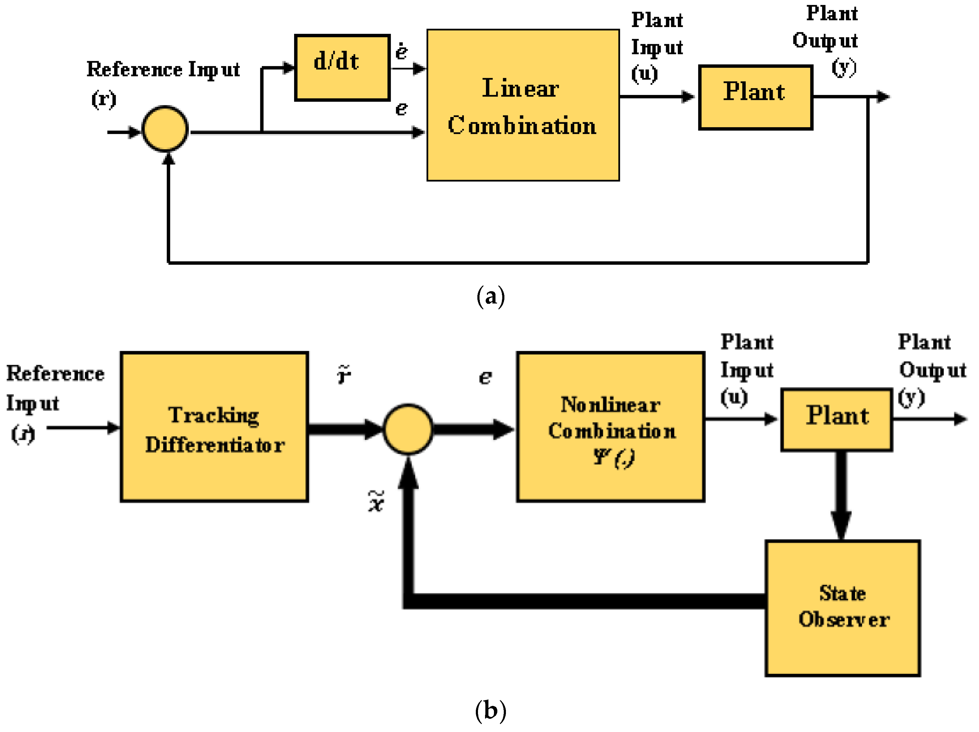
2.1. The Improved Nonlinear TD (INTD)
- The function is smooth, i.e., ;
- is an odd function;
- The function satisfies .
- (i)
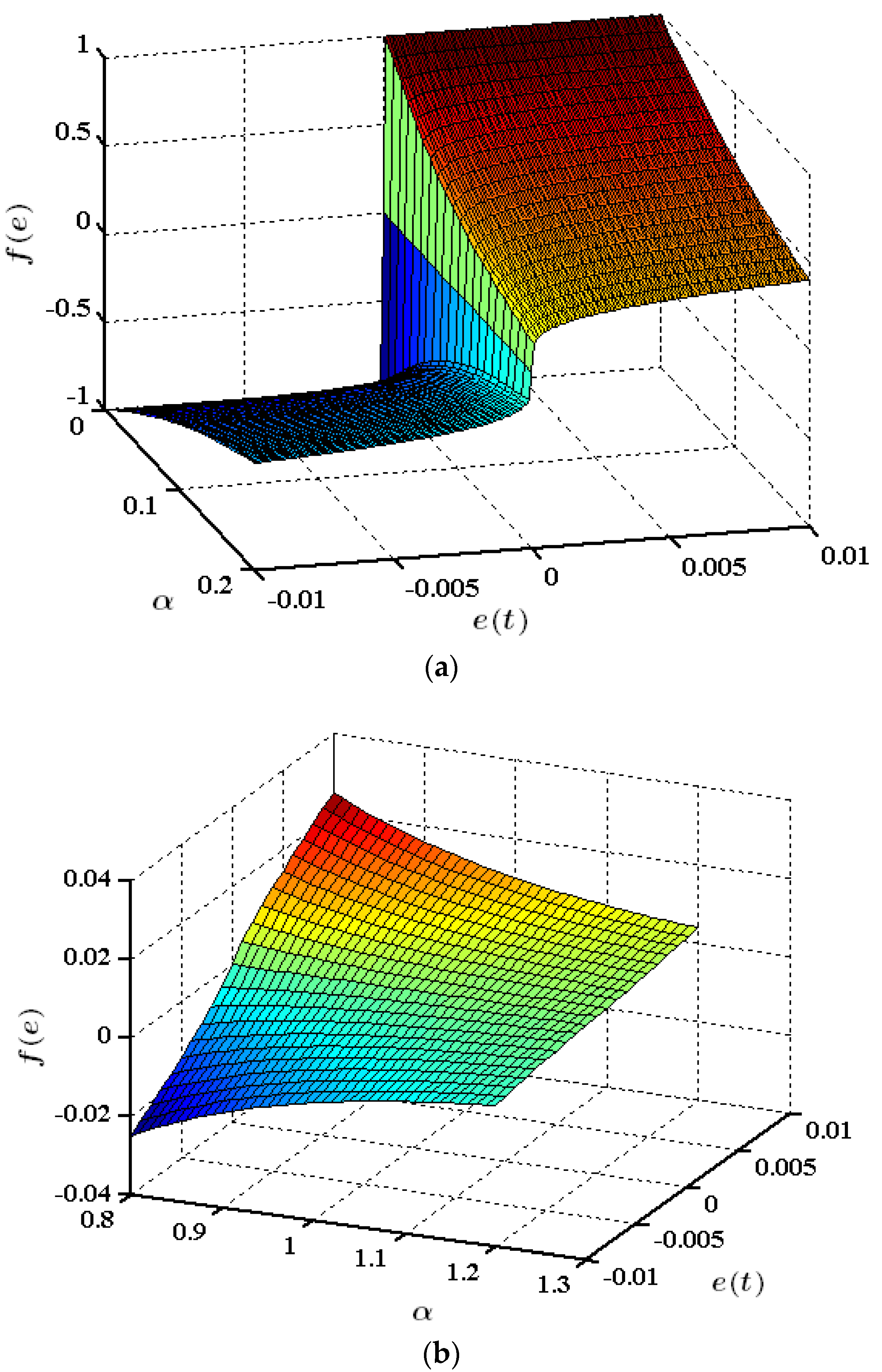
- The proposed tracking differentiator is built using a smooth nonlinear function () instead of the function used in most conventional nonlinear differentiators. This is an essential step toward preventing a chattering phenomenon from the output derivatives;
- (ii)
- A second improvement is accomplished by combining the linear and the nonlinear terms. The benefits of this are clear in suppressing high-frequency components in the signal, such as noise. With this feature, the proposed GTD also achieves better performance than other tracking differentiators;
- (iii)
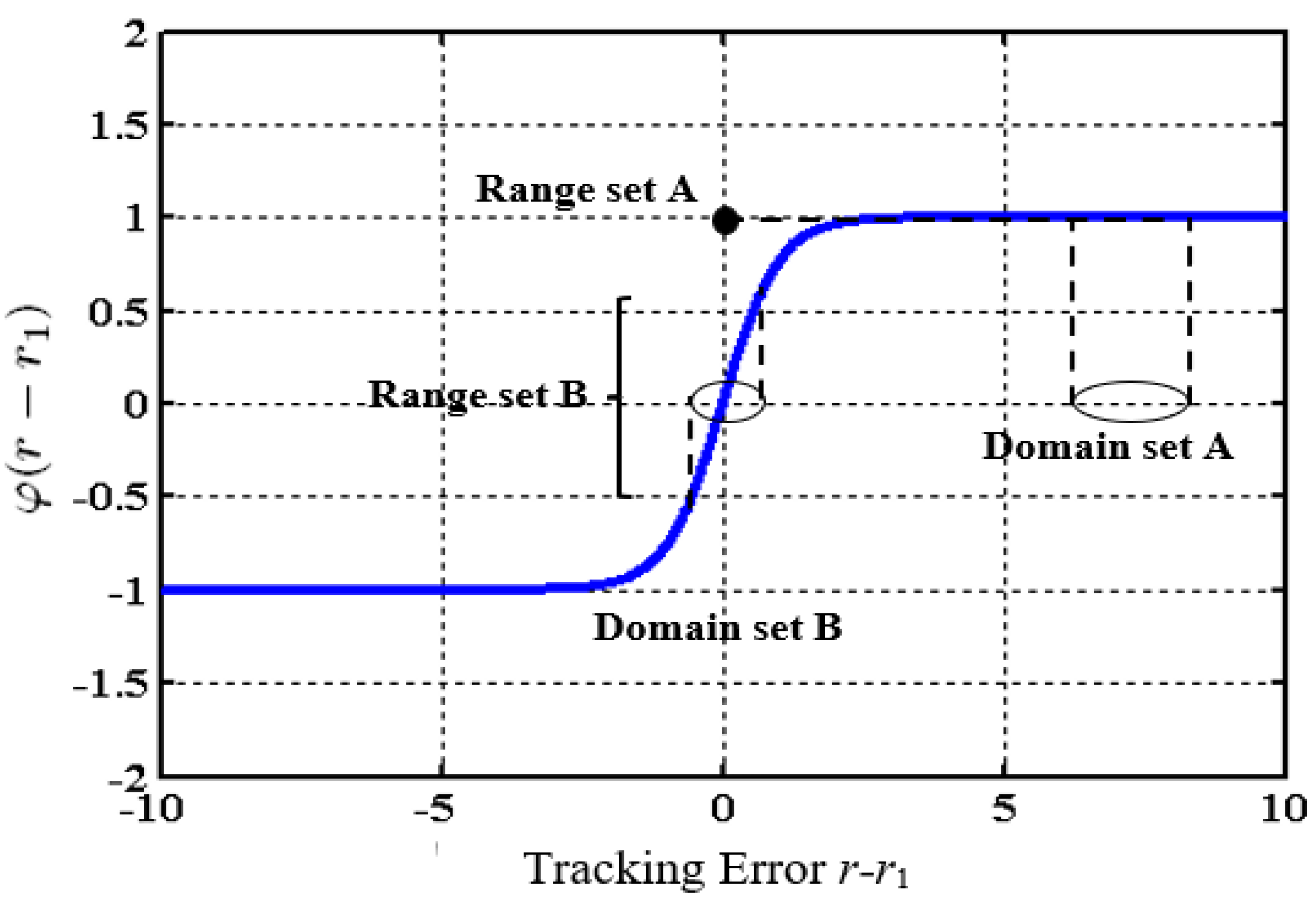
- The saturation feature of the function increases the robustness against noisy signals because for large errors, even with a wide range of noise, it is mapped to a small domain set of the function (see Figure 2, range and domain sets A);
- (iv)
- Increasing the slope of the continuous function near the origin significantly accelerates the convergence of the proposed tracking differentiator (see Figure 2, range and domain sets B).
2.2. The Improved Nonlinear State Error Feedback Controller (INSEFC)
- The closed-loop system is asymptotically stable in the presence of external disturbances, system uncertainties, and measurement noise;
- The output () is forced to track a known reference signal (), i.e.,, satisfying the transient response specifications;
- The chattering phenomenon in the control signal () is reduced.
- (i)
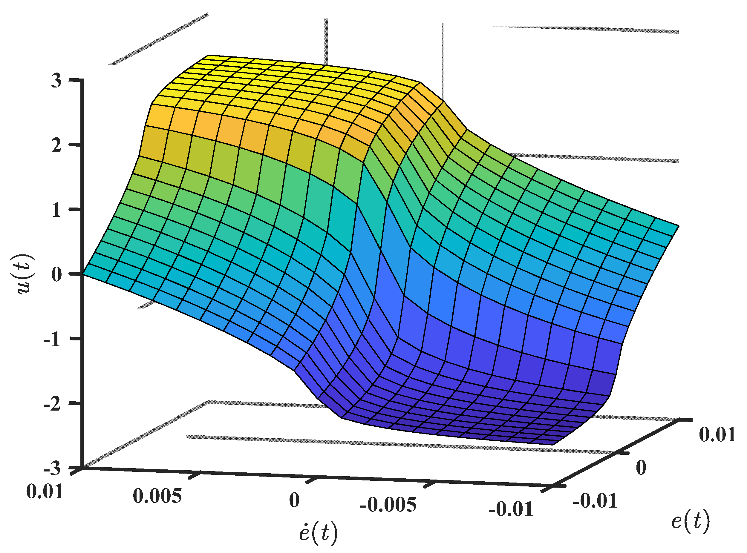
- Any real number is mapped to a number in the range of ;
- (ii)
- The function is symmetric about the origin, and only zero-valued inputs are mapped to zero outputs;
- (iii)
- The control action (u) is limited via mapping but not clipped. Therefore, there are no strong harmonics in the high-frequency range.
2.3. Sliding Mode Extended State Observer (SMESO)
3. Convergence and Stability Analysis
3.1. Convergence Analysis of the Proposed SMESO
- (i)
- (ii)
3.2. Stability Analysis of the Closed-Loop System
4. Mismatched Disturbances
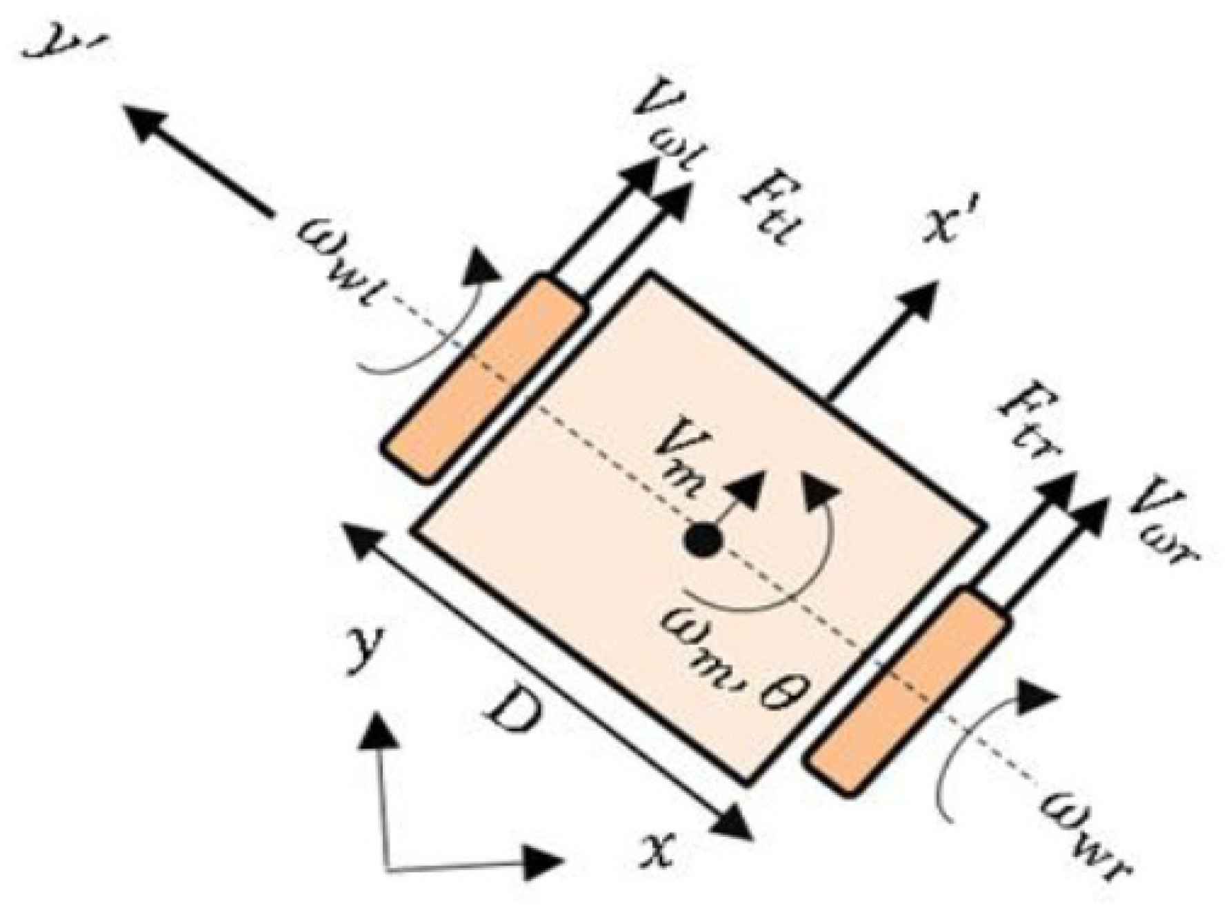
5. Mathematical Modelling of The Differential Drive Mobile Robot
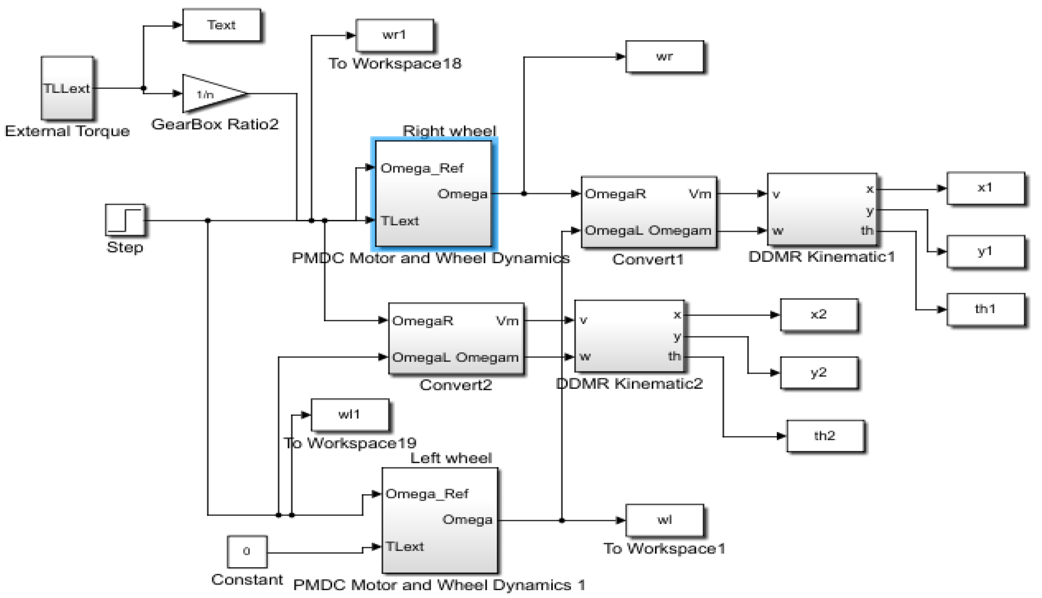
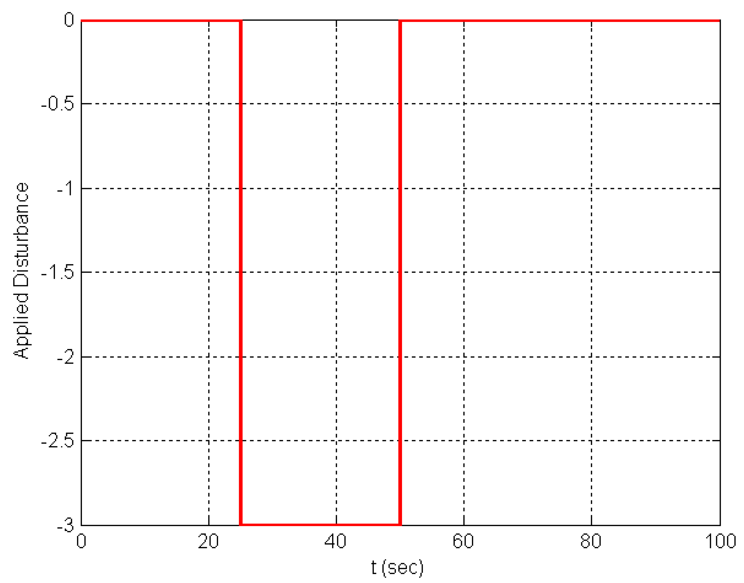
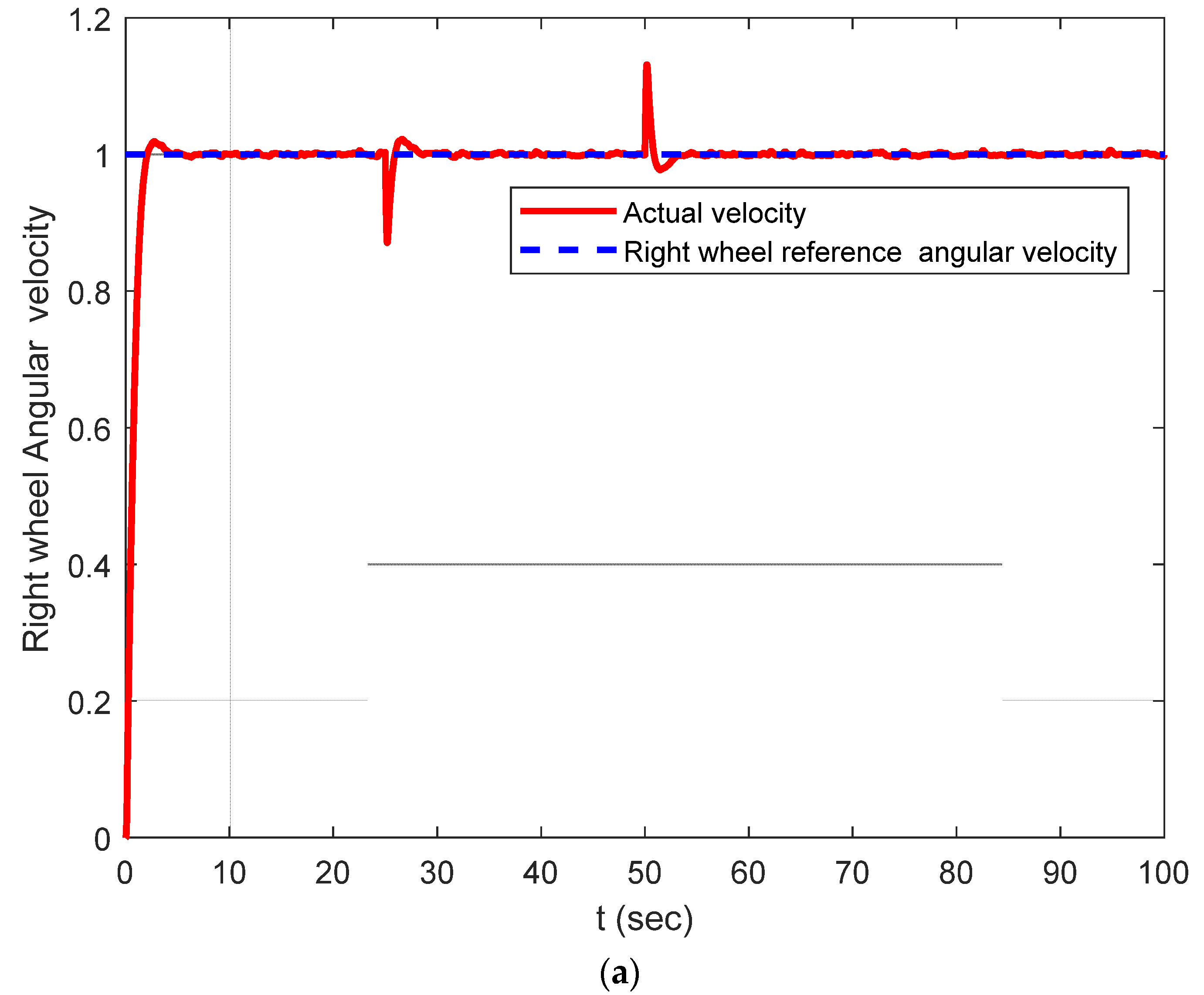
6. Numerical Simulations
- where ,
- ,
Discussion
7. Conclusions
Author Contributions
Funding
Institutional Review Board Statement
Data Availability Statement
Acknowledgments
Conflicts of Interest
References
- Åström, K.; Hägglund, T. Advanced PID Control; ISA Press: Durham, NC, USA, 2006. [Google Scholar]
- Seborg, D.E.; Edgar, T.E. Process Dynamics and Control, 2nd ed.; Wiley: Cambridge, MA, USA, 2004. [Google Scholar]
- Han, J. Extended state observer for a class of uncertain plants. Control Decis. 1995, 10, 85–88. (In Chinese) [Google Scholar]
- Han, J. From PID to active disturbance rejection control. IEEE Trans. Ind. Electron. 2009, 56, 900–906. [Google Scholar] [CrossRef]
- Zhang, C.; Chen, Y. Tracking Control of Ball Screw Drives Using ADRC and Equivalent-Error-Model-Based Feedforward Control. IEEE Trans. Ind. Electron. 2016, 63, 7682–7692. [Google Scholar] [CrossRef]
- Shi, M.; Liu, X.; Shi, Y. Research n Enhanced ADRC algorithm for hydraulic active suspension. In Proceedings of the International Conference on Transportation, Mechanical, and Electrical Engineering (TMEE), Changchun, China, 16–18 December 2011. [Google Scholar] [CrossRef]
- Chenlu, W.; Zengqiang, C.; Qinglin, S.; Qing, Z. Design of PID and ADRC based quadrotor helicopter control system. In Proceedings of the Control and Decision Conference (CCDC), Yinchuan, China, 28–30 May 2016. [Google Scholar] [CrossRef]
- Wu, Y.; Zheng, Q. ADRC or adaptive controller—A simulation study on artificial blood pump. Comput. Biol. Med. 2015, 66, 135–143. [Google Scholar] [CrossRef]
- Rahman, M.M.; Chowdhury, A.H. Comparative study of ADRC and PID based Load Frequency Control. In Proceedings of the International Conference on Electrical Engineering and Information Communication Technology (ICEEICT), Savar, Bangladesh, 21–23 May 2015. [Google Scholar] [CrossRef]
- Ahmed, A.; Asad Ullah, H.; Haider, I.; Tahir, U.; Attique, H. Analysis of Middleware and ADRC based Techniques for Networked Control. In Proceedings of the 16th International Conference on Sciences and Techniques of Automatic Control & Computer Engineering, Monastir, Tunisia, 21–23 December 2015. [Google Scholar]
- Ibraheem, I.K.; Abdul-Adheem, W.R. On the Improved Nonlinear Tracking Differentiator based Nonlinear PID Controller Design. Int. J. Adv. Comput. Sci. Appl. 2016, 7, 234–241. [Google Scholar]
- Abdul-Adheem, W.R.; Ibraheem, I.K. From PID to Nonlinear State Error Feedback Controller. Int. J. Adv. Comput. Sci. Appl. 2017, 8, 2017. [Google Scholar]
- Abdul-Adheem, W.R.; Ibraheem, I.K. Improved Sliding Mode Nonlinear Extended State Observer based Active Disturbance Rejection Control for Uncertain Systems with Unknown Total Disturbance. Int. J. Adv. Comput. Sci. Appl. 2016, 7, 80–93. [Google Scholar]
- Ibraheem, I.K.; Abdul-Adheem, W.R. An Improved Active Disturbance Rejection Control for a Differential Drive Mobile Robot with Mismatched Disturbances and Uncertainties. arXiv 2018, arXiv:1805.12170. [Google Scholar]
- Huang, Y.; Xue, W.C. Active disturbance rejection control: Methodology and theoretical analysis. ISA Trans. 2014, 53, 963–976. [Google Scholar] [CrossRef]
- Guo, B.Z.; Zhao, Z.L. Active Disturbance Rejection Control for Nonlinear Systems: An Introduction; John Wiley & Sons: Singapore/Hoboken, NJ, USA, 2016. [Google Scholar]
- Azar, A.T.; Abed, A.M.; Abdulmajeed, F.A.; Hameed, I.A.; Kamal, N.A.; Jawad, A.J.M.; Abbas, A.H.; Rashed, Z.A.; Hashim, Z.S.; Sahib, M.A.; et al. A New Nonlinear Controller for the Maximum Power Point Tracking of Photovoltaic Systems in Micro Grid Applications Based on Modified Anti-Disturbance Compensation. Sustainability 2022, 14, 10511. [Google Scholar] [CrossRef]
- Menon, A.R.; Mehrotra, K.; Mohan, C.; Ranka, S. Characterization of a Class of Sigmoid Functions with Applications to Neural Networks. Electrical Engineering and Computer Science Technical Reports. 1994. Available online: http://surface.syr.edu/eecs_techreports/152 (accessed on 1 May 2022).
- Khalil, H.K. Nonlinear Systems; Prentice-Hall: Hoboken, NJ, USA, 1996. [Google Scholar]
- Wu, S.; Dong, B.; Ding, G.; Wang, G.; Liu, G.; Li, Y. Backstepping sliding mode force/position control for constrained reconfigurable manipulator based on extended state observer. In Proceedings of the 12th World Congress on Intelligent Control and Automation (WCICA), Guilin, China, 12–15 June 2016; pp. 477–482. [Google Scholar]
- Yang, H.; Yu, Y.; Yuan, Y.; Fan, X. Back-stepping control of two-link flexible manipulator based on an extended state observer. Adv. Sp. Res. 2015, 56, 2312–2322. [Google Scholar] [CrossRef]
- Xia, Y.; Yang, H.; You, X.; Li, H. Adaptive control for attitude synchronisation of spacecraft formation via extended state observer. IET Control Theory Appl. 2014, 8, 2171–2185. [Google Scholar]
- Lin, Y.P.; Lin, C.L.; Suebsaiprom, P.; Hsieh, S.L. Estimating evasive acceleration for ballistic targets using an extended state observer. IEEE Trans. Aerosp. Electron. Syst. 2016, 52, 337–349. [Google Scholar] [CrossRef]
- Duan, H.; Tian, Y.; Wang, G. Trajectory Tracking Control of Ball and Plate System Based on Auto-Disturbance Rejection Controller. In Proceedings of the 7th Asian Control Conference, Hong Kong, China, 27–29 August 2009; pp. 471–476. [Google Scholar]
- Dejun, L.; Changjin, C.; Zhenxiong, Z. Permanent magnet synchronous motor control system based on auto disturbances rejection controller. In Proceedings of the International Conference on Mechatronic Science, Electric Engineering and Computer (MEC), Jilin, China, 8–11 August 2011. [Google Scholar]
- Liu, B.; Jin, Y.; Chen, C.; Yang, H. Speed Control Based on ESO for the Pitching Axis of Satellite Cameras. Math. Probl. Eng. 2016, 2016, 2138190. [Google Scholar] [CrossRef] [Green Version]
- Li, J.; Xia, Y.; Qi, X.; Gao, Z. On the Necessity, Scheme, and Basis of the Linear-Nonlinear Switching in Active Disturbance Rejection Control. IEEE Trans. Ind. Electron. 2017, 64, 1425–1435. [Google Scholar] [CrossRef]
- Chen, Z.; Xu, D. Output Regulation and Active Disturbance Rejection Control: Unified Formulation and Comparison. Asian J. Control 2015, 18, 1668–1678. [Google Scholar] [CrossRef]
- Xue, W.; Huang, Y. On performance analysis of ADRC for a class of MIMO lower-triangular nonlinear uncertain systems. ISA Trans. 2014, 53, 955–962. [Google Scholar] [CrossRef]
- Yang, J.; Ding, Z. Global output regulation for a class of lower triangular nonlinear systems: A feedback domination approach. Automatica 2017, 76, 65–69. [Google Scholar] [CrossRef] [Green Version]
- Guo, B.-Z.; Wu, Z.-H. Output tracking for a class of nonlinear systems with mismatched uncertainties by active disturbance rejection control. Syst. Control Lett. 2017, 100, 21–31. [Google Scholar] [CrossRef]
- Qian, C.; Li, S.; Frye, M.T.; Du, H. Global finite-time stabilisation using bounded feedback for a class of non-linear systems. IET Control Theory Appl. 2012, 6, 2326–2336. [Google Scholar]
- Zhu, Q. Stabilization of stochastic nonlinear delay systems with exogenous disturbances and the event-triggered feedback control. IEEE Trans. Autom. Control 2019, 64, 3764–3771. [Google Scholar] [CrossRef]
- Ding, K.; Zhu, Q. Extended dissipative anti-disturbance control for delayed switched singular semi-Markovian jump systems with multi-disturbance via disturbance observer. Automatica 2021, 128, 109556. [Google Scholar] [CrossRef]
- Yang, X.; Wang, H.; Zhu, Q. Event-triggered predictive control of nonlinear stochastic systems with output delay. Automatica 2020, 140, 110230. [Google Scholar] [CrossRef]
- Cerkala, J.; Jadlovska, A. Nonholonomic Mobile Robot with Differential Chassis Mathematical Modelling And Implementation In Simulink with Friction in Dynamics. Acta Electrotech. Et Inform. 2015, 15, 3–8. [Google Scholar] [CrossRef]
- Salem, F.A. Dynamic and Kinematic Models and Control for Differential Drive Mobile Robots. Int. J. Curr. Eng. Technol. 2013, 3, 253–263. [Google Scholar]
- Dhaouadi, R.; Hatab, A.A. Dynamic Modelling of Differential-Drive Mobile Robots using Lagrange and Newton-Euler Methodologies: A Unified Framework. Adv. Robot Autom. 2013, 2, 107. [Google Scholar]
- Sousa, R.L.S.; Forte, M.D.D.N.; Nogueira, F.G.; Torrico, B.C. Trajectory Tracking Control of a Nonholonomic Mobile Robot with Differential Drive. In Proceedings of the Biennial Congress of Argentina (ARGENCON), Buenos Aires, Argentina, 15–17 June 2016. [Google Scholar] [CrossRef]
- Ajeil, F.; Ibraheem, I.K.; Azar, A.T.; Humaidi, A.J. Autonomous Navigation and Obstacle Avoidance of an Omnidirectional Mobile Robot Using Swarm Optimization and Sensors Deployment. Int. J. Adv. Robot. Syst. 2020, 17, 1729881420929498. [Google Scholar] [CrossRef]
- Ammar, H.H.; Azar, A.T. Robust Path Tracking of Mobile Robot Using Fractional Order PID Controller. In Proceedings of the International Conference on Advanced Machine Learning Technologies and Applications (AMLTA2019), Cairo, Egypt, 28–30 March 2019; Hassanien, A., Azar, A., Gaber, T., Bhatnagar, R.F., Tolba, M., Eds.; Advances in Intelligent Systems and Computing. Springer: Cham, Switzerland, 2020; Volume 921, pp. 370–381. [Google Scholar]
- Zidani, G.; Drid, S.; Chrifi-Alaoui, L.; Benmakhlouf, A.; Chaouch, S. Backstepping Controller for a Wheeled Mobile Robot. In Proceedings of the 4th International Conference on Systems and Control, Sousse, Tunisia, 28–30 April 2015. [Google Scholar]


| Performance Index | Controller | |
|---|---|---|
| ADRC | IADRC | |
| 0.0010884970 | 0.0005257305 | |
| 0.0016112239 | 0.0007447036 | |
| 0.0000059780 | 0.0000017459 | |
| Wheel | Performance Index | Controller | |
|---|---|---|---|
| ADRC | IADRC | ||
| Right | 13.302889 | 1.780254 | |
| 1372.090423 | 1407.300305 | ||
| Left | 6.919226 | 0.146694 | |
| 1343.542226 | 1372.124019 | ||
Disclaimer/Publisher’s Note: The statements, opinions and data contained in all publications are solely those of the individual author(s) and contributor(s) and not of MDPI and/or the editor(s). MDPI and/or the editor(s) disclaim responsibility for any injury to people or property resulting from any ideas, methods, instructions or products referred to in the content. |
© 2023 by the authors. Licensee MDPI, Basel, Switzerland. This article is an open access article distributed under the terms and conditions of the Creative Commons Attribution (CC BY) license (https://creativecommons.org/licenses/by/4.0/).
Share and Cite
Hameed, I.A.; Abbud, L.H.; Abdulsaheb, J.A.; Azar, A.T.; Mezher, M.; Jawad, A.J.M.; Abdul-Adheem, W.R.; Ibraheem, I.K.; Kamal, N.A. A New Nonlinear Dynamic Speed Controller for a Differential Drive Mobile Robot. Entropy 2023, 25, 514. https://doi.org/10.3390/e25030514
Hameed IA, Abbud LH, Abdulsaheb JA, Azar AT, Mezher M, Jawad AJM, Abdul-Adheem WR, Ibraheem IK, Kamal NA. A New Nonlinear Dynamic Speed Controller for a Differential Drive Mobile Robot. Entropy. 2023; 25(3):514. https://doi.org/10.3390/e25030514
Chicago/Turabian StyleHameed, Ibrahim A., Luay Hashem Abbud, Jaafar Ahmed Abdulsaheb, Ahmad Taher Azar, Mohanad Mezher, Anwar Ja’afar Mohamad Jawad, Wameedh Riyadh Abdul-Adheem, Ibraheem Kasim Ibraheem, and Nashwa Ahmad Kamal. 2023. "A New Nonlinear Dynamic Speed Controller for a Differential Drive Mobile Robot" Entropy 25, no. 3: 514. https://doi.org/10.3390/e25030514