Clustering Matrix Variate Longitudinal Count Data

Abstract

Matrix variate longitudinal discrete data can arise in transcriptomics studies when the data are collected for N genes at r conditions over t time points, and thus, each observation ${\mathbf{Y}}_n$ for $n=1,\dots ,N$ can be written as an $r\times t$ matrix. When dealing with such data, the number of parameters in the model can be greatly reduced by considering the matrix variate structure. The components of the covariance matrix then also provide a meaningful interpretation. In this work, a mixture of matrix variate Poisson-log normal distributions is introduced for clustering longitudinal read counts from RNA-seq studies. To account for the longitudinal nature of the data, a modified Cholesky-decomposition is utilized for a component of the covariance structure. Furthermore, a parsimonious family of models is developed by imposing constraints on elements of these decompositions. The models are applied to both real and simulated data, and it is demonstrated that the proposed approach can recover the underlying cluster structure.

1. Introduction

Biological studies are a major source of longitudinal data. While modelling such longitudinal datasets, it is important to take into account the correlations among the measurements at different time points. Gene expression time course studies present important clustering and classification problems. Understanding how different genes are modulated over a period of time during an event of interest can provide key insight in understanding their involvement in various biological pathways [1,2,3,4]. Cluster analysis allows us to group genes into clusters with similar patterns, or ‘expression profiles’, over time.

Model-based clustering approaches have been shown to be an effective approach for clustering a wide variety of biological datasets, such as microarray datasets [5,6,7], RNA-seq data [8,9,10], microbiome data [11,12], flow cytometry data [13,14], etc. Several studies have utilized cluster analysis to gain novel insights into various biological phenomenon, such as identification of novel tumour subtypes [15,16], understanding diseases progression [17,18], understanding crops’ response to abiotic stresses [19,20], and others.

Model-based clustering utilizes finite mixture models [21] for cluster analysis, which assumes that a population is a mixture of G subpopulations or components and each component can be modelled using a probability distribution. A random vector $\mathbf{Y}$ is said to arise from a parametric finite mixture distribution; we can write its density in the form

$$f(\mathbf{y}\mid \mathbf{\Theta })=\sum _{g=1}^G{\pi }_{g}f(\mathbf{y}\mid {\mathit{\theta }}_g)$$

(1)

where ${\pi }_g\in [0,1]$ such that ${\sum }_{g=1}^G{\pi }_g=1$ is the mixing proportion of the $g\mathrm{t}\mathrm{h}$ component, $\mathrm{f}(\mathbf{y}\mid {\mathit{\theta }}_g)$ is the density of the $g\mathrm{t}\mathrm{h}$ component, and $\mathbf{\Theta }=({\pi }_1,\dots ,{\pi }_G,{\mathit{\theta }}_1,\dots ,{\mathit{\theta }}_G)$ are the model parameters. The choice of an appropriate probability density/mass function depends on the data type.

Various approaches have been developed for the clustering of time course gene expression data (e.g., [6,7,22,23,24,25]). However, most statistical approaches for clustering gene expression data are tailored for microarray studies. While some of this could be attributed to RNA-seq technology being more recent compared to microarrays, the computational cost that comes with fitting multivariate discrete models needed for RNA-seq data has also led to challenges. The transcriptomics data arising from RNA-seq studies are discrete, high-dimensional, and over-dispersed count data. Efficiently analyzing these data remains a challenge. Because of the restrictive mean-variance relationship that comes with the Poisson distribution, the negative binomial distribution emerged as the univariate distribution of choice [26,27]. However, the multivariate negative binomial distribution [28] is seldom used in practice due to the computational cost that comes with fitting such a model [29].

Recently, [10] proposed mixtures of multivariate Poisson lognormal (MPLN) models for clustering over-dispersed, multivariate count data. In the MPLN model, the counts of the $n\mathrm{t}\mathrm{h}$ gene (with $n=1,2,\dots ,N$) are modelled using a hierarchical Poisson log-normal distribution such that $Y_{nj}\sim \mathrm{Poisson}\left(e^{X_{nj}+\log c_j}\right)$ and ${\mathbf{X}}_n\sim {\mathcal{N}}_p(\mathit{\mu },\mathbf{\Sigma }),$ where ${\mathbf{X}}_n=(X_{n1},X_{n2},\dots ,X_{np})$, ${\mathcal{N}}_p(\mathit{\mu },\mathbf{\Sigma })$ denotes a p-dimensional Gaussian distribution with mean $\mathit{\mu }$ and covariance $\mathbf{\Sigma }$, and $c_j$ is a known constant representing the normalized library size of the $j\mathrm{t}\mathrm{h}$ sample. This hierarchical structure allows for over-dispersion similar to the negative binomial distribution, but it also allows for correlation between the variables. An efficient framework for parameter estimation for mixtures of MPLN distributions was developed by [30] that utilizes a variational Gaussian approximation.

In RNA-seq studies, it is common to obtain expression levels of n genes at r conditions over t occasions in one study. A natural framework for modelling such data is a matrix variate approach such that each observation ${\mathbf{Y}}_n$ is a $r\times t$ matrix. Alternately, a multivariate framework can also be utilized, where each observation ${\mathbf{Y}}_n$ can be written as a vector $\mathrm{vec}\left({\mathbf{Y}}_n^{\prime }\right)$ of dimensionality $rt=r\times t$. In [31], the authors developed mixtures of matrix variate Poisson lognormal distributions (MVPLN). In the MVPLN model, $Y_{n,ij}\sim \mathrm{Poisson}\left(e^{X_{n,ij}+\log C_{ij}}\right)$ and ${\mathbf{X}}_n\sim {\mathcal{N}}_{r\times t}(\mathbf{M},\mathbf{\Phi },\mathbf{\Omega })$, where ${\mathbf{X}}_n$ is an $r\times t$ matrix, and ${\mathcal{N}}_{r\times t}(\mathbf{M},\mathbf{\Phi },\mathbf{\Omega })$ denotes a matrix normal distribution with location matrix $\mathbf{M}$ and scale matrices $\mathbf{\Phi }$ and $\mathbf{\Omega }$, and $\mathbf{C}$ is a $r\times t$ matrix where $C_{ij}$ denotes the normalized library size of the $i\mathrm{t}\mathrm{h}$ condition from the $j\mathrm{t}\mathrm{h}$ time point. Mathematically, the MVPLN model is equivalent to $Y_{n,ij}\sim \mathrm{Poisson}\left(e^{X_{n,ij}+\log C_{ij}}\right)$ and $\mathrm{vec}\left({\mathbf{X}}_n^{\prime }\right)\sim {\mathcal{N}}_{rt}(\mathrm{vec}\left({\mathbf{M}}^{\prime }\right),\mathbf{\Sigma }=\mathbf{\Phi }\otimes \mathbf{\Omega })$, where ${\mathcal{N}}_{rt}$ is an $rt$-dimensional multivariate normal distribution and ⊗ is a Kronecker product. By adopting a matrix variate form, the large $rt\times rt$ covariance matrix of the latent variable $\mathbf{X}$ can be written as the Kronecker product of two smaller $r\times r$ and $t\times t$ scale matrices $\mathbf{\Phi }$ and $\mathbf{\Omega }$, i.e., ${\mathbf{\Sigma }}_{rt\times rt}={\mathbf{\Phi }}_{r\times r}\otimes {\mathbf{\Omega }}_{t\times t}$. This can greatly reduce the number of parameters in $\mathbf{\Sigma }$.

In Section 2, we extend the mixtures of the matrix variate Poisson log-normal model for clustering matrix variate longitudinal RNA-seq data by incorporating a modified Cholesky decomposition of the scale matrix $\mathbf{\Omega }$ that captures the covariances of the t occasions of the latent variable $\mathbf{X}$. Furthermore, by imposing constraints on the components of scale matrices to be equal or different across the group, a family of eight models is obtained. Parameter estimation is performed using a variational variant of the expectation-maximization algorithm. In Section 3, the proposed models are applied to simulated and real datasets, and Section 4 concludes the paper.

2. Methods

A matrix variate Poisson log-normal distribution was proposed by [31] for modelling RNA-seq data. This arises from a hierarchical mixture of independent Poisson distributions with a matrix variate Gaussian distribution. Suppose ${\mathbf{Y}}_1,\dots ,{\mathbf{Y}}_N$ are N observations from a matrix variate Poisson log-normal distribution, where the $n\mathrm{t}\mathrm{h}$ observation ${\mathbf{Y}}_n$ is an $r\times t$ dimensional matrix representing r conditions and t time points. A matrix variate Poisson log-normal distribution for modelling RNA-seq data can be written as

$$\begin{array}{c}\hfill Y_{n,ij}\mid X_{n,ij}\sim \mathrm{Poisson}\left(e^{X_{n,ij}+\log C_{ij}}\right), \mathrm{and} {\mathbf{X}}_n\sim {\mathcal{N}}_{r\times t}(\mathbf{M},\mathbf{\Phi },\mathbf{\Omega }),\end{array}$$

(2)

where $\mathbf{M}$ is an $r\times t$ matrix of means, $\mathbf{C}$ is an $r\times t$ matrix of fixed, known constants to account for the differences in library sizes across each sample, and $\mathbf{\Phi }$ and $\mathbf{\Omega }$ are $r\times r$ and $t\times t$ scale matrices, respectively. Suppose the least-squares predictor of unobserved latent variable $X_{n,ij}$ of the $n\mathrm{t}\mathrm{h}$ observation from the $i\mathrm{t}\mathrm{h}$ condition at the $j\mathrm{t}\mathrm{h}$ time point can be written as

$$\begin{array}{c}\hfill {\widehat{X}}_{n,ij}=M_{ij}+\sum _{k=1}^{j-1}(-{\rho }_{jk})(X_{n,ik}-M_{ik})+\sqrt{d_j}{\epsilon }_j,\end{array}$$

(3)

where $X_{n,i1}$, $X_{n,i2}$,…, $X_{n,i(j-1)}$ are the unobserved latent variables from the preceding $j-1$ time points, ${\epsilon }_j\sim \mathcal{N}(0,1)$, and ${\rho }_{jk}$ and $d_j$ are the autoregressive parameters and innovation variances, respectively [32]. Thus, when the responses are recorded over a period of time (i.e., t time points), the parameter $\mathbf{\Omega }$ that relates to the covariance of the t time points can be parameterized to account for the relationship between measurements at different time points. Now, $\mathbf{\Omega }$ can be decomposed using the modified Cholesky decomposition [7,23,32] such that $\mathbf{T}\mathbf{\Omega }{\mathbf{T}}^{\prime }=\mathbf{D}$. This can alternately be written as ${\mathbf{\Omega }}^{-1}={\mathbf{T}}^{\prime }{\mathbf{D}}^{-1}\mathbf{T}$, where $\mathbf{D}$ is a unique diagonal matrix with innovation variances $d_1,\dots ,d_t$, and $\mathbf{T}$ is a unique lower triangular matrix with 1 as the diagonal elements and the autoregressive parameters (${\rho }_{jk}$ with $j>k$) as the off-diagonal elements:

$$\mathbf{T}=\left(\begin{array}{cccc}1& 0& \dots & 0\\ {\rho }_{12}& 1& \dots & 0\\ \dots & \dots & & \dots \\ {\rho }_{j,j-1}& {\rho }_{2,j-1}& \dots & 1\end{array}\right).$$

In the context of a G-component mixture of matrix variate Poisson log-normal distributions [31], Equation (1) can be written as

$$f(\mathbf{Y}\mid \mathbf{\Theta })=\sum _{g=1}^G{\pi }_{g}f(\mathbf{Y}\mid {\mathbf{M}}_g,{\mathbf{\Phi }}_g,{\mathbf{\Omega }}_g),$$

where ${\pi }_g>0$ is the mixing proportion of the $g\mathrm{t}\mathrm{h}$ component such that ${\sum }_{g=1}^G{\pi }_g=1$, and $f(\mathbf{Y}\mid {\mathbf{M}}_g,{\mathbf{\Phi }}_g,{\mathbf{\Omega }}_g)$ is the marginal distribution function of the $g\mathrm{t}\mathrm{h}$ component with parameters ${\mathbf{M}}_g$, ${\mathbf{\Phi }}_g$, and ${\mathbf{\Omega }}_g$, and $\mathbf{\Theta }$ denotes all the model parameters.

2.1. Longitudinal Data and Family of Models

Due to the longitudinal nature of t time points, one can utilize the modified Cholesky decomposition for ${\mathbf{\Omega }}_g$ such that ${\mathbf{\Omega }}_g^{-1}={\mathbf{T}}_g^{\prime }{\mathbf{D}}_g^{-1}{\mathbf{T}}_g$. The number of parameters in ${\mathbf{\Omega }}_g$ (i.e., $t(t+1)/2$) increases quadratically with respect to time points, and this is further compounded in mixture models as G different $\mathbf{\Omega }$s need to be estimated. Thus, similar to [7], constraints can be imposed on ${\mathbf{T}}_g$ and ${\mathbf{D}}_g$ to be equal or different across groups, and an isotropic constraint can also be imposed on ${\mathbf{D}}_g={\delta }_g\mathbf{I}$, where ${\delta }_g$ is a scalar. Various combinations of these constraints result in a family of eight models (see

Table 1. The family of eight models obtained by imposing various constraints on the components of ${\mathbf{\Omega }}_g$.

Model	${\mathbf{T}}_{\mathit{g}}$	${\mathbf{D}}_{\mathit{g}}$		Total Parameters in ${\mathbf{\Omega }}_1,\mathbf{\dots },{\mathbf{\Omega }}_{\mathit{G}}.$
	Group	Group	Diagonal
“VVA”	Variable	Variable	Anisotropic	$Gt(t-1)/2+Gt$
“EVA”	Equal	Variable	Anisotropic	$t(t-1)/2+Gt$
“VEA”	Variable	Equal	Anisotropic	$Gt(t-1)/2+t$
“EEA”	Equal	Equal	Anisotropic	$t(t-1)/2+t$
“VVI”	Variable	Variable	Isotropic	$Gt(t-1)/2+G$
“EVI”	Equal	Variable	Isotropic	$t(t-1)/2+G$
“VEI”	Variable	Equal	Isotropic	$Gt(t-1)/2+1$
“EEI”	Equal	Equal	Isotropic	$t(t-1)/2+1$

).

Parameter estimation is outlined in Section 2.2. In cluster analysis, the best constraint for a specific dataset is also unknown. Selection of the best fitting model among the eight models in the family for a given dataset is performed using a model selection criteria, which is discussed in detail in Section 2.3.

2.2. Parameter Estimation

Parameter estimation for mixture models is typically conducted using the traditional expectation-maximization (EM; [33]) algorithm. In the case of an MVPLN model, this requires computing the posterior expectations of $\mathbb{E}(\mathbf{X}\mid \mathbf{Y})$ and $\mathbb{E}(\mathbf{X}{\mathbf{X}}^{\prime }\mid \mathbf{Y})$. However, the posterior distribution of a latent variable (i.e., $\mathbf{X}\mid \mathbf{Y}$) does not have a known form; thus, a Markov chain Monte Carlo expectation-maximization (MCMC-EM) algorithm is typically employed for empirically estimating $\mathbb{E}(\mathbf{X}\mid \mathbf{Y})$ and $\mathbb{E}(\mathbf{X}{\mathbf{X}}^{\prime }\mid \mathbf{Y})$. Such an approach can be computationally intensive [10,31].

Subedi and Browne [30] developed an efficient parameter estimation algorithm for a matrix variate Poisson log-normal distribution using variational approximations [34]. This utilized a computationally convenient approximating density to approximate a more complex but ‘true’ posterior density through minimization of the Kullback– Leibler (KL) divergence between the true and the approximating densities. Suppose we have an approximating density $q\left(\mathbf{X}\right)$; then, the marginal log of the probability mass function can be written as $\log f_Y\left(\mathbf{Y}\right)=F(q,\mathbf{Y})+D_{KL}(q\parallel f),$ where $D_{KL}(q\parallel f)=\int q\left(\mathbf{X}\right)\log \frac{q\left(\mathbf{X}\right)}{f(\mathbf{X}\mid \mathbf{Y})}d\mathbf{X}$ is the KL divergence between $f(\mathbf{X}\mid \mathbf{Y})$, and the approximating distribution $q\left(\mathbf{X}\right)$, and $F(q,\mathbf{Y})=\int \left[\log f\right(\mathbf{Y},\mathbf{X})-\log q(\mathbf{X}\left)\right]q\left(\mathbf{X}\right)d\mathbf{X}$ is our evidence lower bound (ELBO). A Gaussian density is utilized as the approximating density for variational Gaussian approximations. Similar to [31], assuming $q\left({\mathbf{X}}_{ng}\right)=N_{r\times t}({\mathbf{\xi }}_{ng},{\mathbf{\Delta }}_{ng},{\mathbf{\kappa }}_{ng})$, the ELBO for each observation ${\mathbf{y}}_n$ from the $g\mathrm{t}\mathrm{h}$ component can be written as

$$\begin{array}{c}F(q_{ng},{\mathbf{Y}}_n)=-\left[\sum _{i=1}^r\sum _{j=1}^t\exp \left\{{\left({\mathbf{\xi }}_{ng}\right)}_{ij}+\frac{1}{2}{\left({\mathbf{\Delta }}_{ng}\right)}_{ii}{\left({\mathbf{\Omega }}_{ng}\right)}_{jj}+\log C_{ij}\right\}\right]\hfill \\ +{\left[\mathrm{vec}\left({\mathbf{\xi }}_{ng}^{\prime }\right)+\log \mathrm{vec}\left({\mathbf{C}}^{\prime }\right)\right]}^{\prime }\mathrm{vec}\left({\mathbf{Y}}_n^{\prime }\right)-\left[\sum _{k=1}^{rt}\log (\mathrm{vec}{\left({\mathbf{Y}}_n^{\prime }\right)}_k!)\right]-\frac{p}{2}\log |{\mathbf{\Phi }}_g|-\frac{r}{2}\log \left|{\mathbf{T}}_g^{\prime }{\mathbf{D}}_g^{-1}{\mathbf{T}}_g\right|\hfill \\ -\frac{1}{2}{\left(\mathrm{vec}\left({\mathbf{\xi }}_{ng}^{\prime }\right)-\mathrm{vec}\left({\mathbf{M}}_g^{\prime }\right)\right)}^{\prime }{\mathbf{\Phi }}_g^{-1}\otimes \left({\mathbf{T}}_g^{\prime }{\mathbf{D}}_g^{-1}{\mathbf{T}}_g\right)\left(\mathrm{vec}\left({\mathbf{\xi }}_{ng}^{\prime }\right)-\mathrm{vec}\left({\mathbf{M}}_g^{\prime }\right)\right)\hfill \\ +\mathrm{tr}\left\{{\mathbf{\Phi }}_g^{-1}{\mathbf{\Delta }}_{ng}\right\}\mathrm{tr}\left\{{\mathbf{T}}_g^{\prime }{\mathbf{D}}_g^{-1}{\mathbf{T}}_g{\mathbf{\kappa }}_{ng}\right\}+\frac{t}{2}\log |{\mathbf{\Delta }}_{ng}|+\frac{r}{2}\log \left|{\mathbf{\kappa }}_{ng}\right|+\frac{rt}{2}.\hfill \end{array}$$

Thus, the complete-data log-likelihood for the mixtures of MVPLN distributions can be written as

$$\begin{array}{c}{l}_c\left(\mathbf{\Theta }\right)=\sum _{g=1}^G\sum _{n=1}^N{z}_{ng}\log {\pi }_g+\sum _{g=1}^G\sum _{n=1}^N{z}_{ng}\log f({\mathbf{Y}}_n\mid {\mathbf{M}}_g,{\mathbf{\Phi }}_g,{\mathbf{T}}_g,{\mathbf{D}}_g)\hfill \\ =\sum _{g=1}^G\sum _{n=1}^N{z}_{ng}\log {\pi }_g+\sum _{g=1}^G\sum _{n=1}^N{z}_{ng}\left[F({\mathbf{Y}}_n,q_{ng})+D_{KL}(q_{ng}\parallel f_{ng})\right],\hfill \end{array}$$

where $D_{KL}(q_{ng}\parallel f_{ng})=\int q\left({\mathbf{X}}_{ng}\right)\log \frac{q\left({\mathbf{X}}_{ng}\right)}{f({\mathbf{X}}_n\mid {\mathbf{Y}}_n,Z_{ng}=1)}d{\mathbf{X}}_{ng}$ is the KL divergence between $f({\mathbf{X}}_n\mid {\mathbf{Y}}_n,Z_{ng}=1)$ and approximating distribution $q\left({\mathbf{X}}_{ng}\right)$. As the variational parameters that maximize the ELBO also minimize the KL divergence, the estimates of the model parameters are obtained by maximizing the variational approximation of the complete-data log-likelihood using the ELBO, i.e.,

$$l_c\left(\mathbf{\Theta }\right)\approx \sum _{g=1}^G\sum _{n=1}^N{z}_{ng}\log {\pi }_g+\sum _{g=1}^G\sum _{n=1}^N{z}_{ng}F({\mathbf{Y}}_n,q_{ng}).$$

Similar to [31], an iterative EM-type algorithm is utilized for parameter estimation. At the $(k+1)\mathrm{t}\mathrm{h}$ step,

• Conditional on the variational parameters ${\mathbf{\xi }}_{ng}$, ${\mathbf{\Delta }}_{ng}$, and ${\mathbf{\kappa }}_{ng}$ and on ${\mathbf{M}}_g$, ${\mathbf{\Phi }}_g$, ${\mathbf{T}}_g$, and ${\mathbf{D}}_g$, the $\mathbb{E}\left(Z_{ng}\right)$ is given by

  $$\begin{array}{c}\hfill \mathbb{E}(Z_{ng}\mid {\mathbf{Y}}_n)=\frac{{\pi }_{g}f({\mathbf{Y}}_n\mid {\mathbf{M}}_g,{\mathbf{\Phi }}_g,{\mathbf{T}}_g,{\mathbf{D}}_g)}{{\sum }_{h=1}^G{\pi }_{h}f({\mathbf{Y}}_n\mid {\mathbf{M}}_h,{\mathbf{\Phi }}_h,{\mathbf{T}}_h,{\mathbf{D}}_h)}.\end{array}$$
  As the marginal distribution of ${\mathbf{Y}}_n$ is difficult to compute, we use an approximation of $\mathbb{E}\left(Z_{ng}\right)$ using the ELBO such that

  $$\begin{array}{c}\hfill {\widehat{Z}}_{ng}^{(k+1)}\stackrel{\mathrm{def}}{=}\frac{{\pi }_g\exp \left[F\left(q_{ng},{\mathbf{Y}}_n\right)\right]}{{\sum }_{h=1}^G{\pi }_h\exp \left[F\left(q_{nh},{\mathbf{Y}}_n\right)\right]}.\end{array}$$

  (4)
• Given ${\widehat{Z}}_{ng}^{(k+1)}$, variational parameters ${\mathbf{\xi }}_{ng}$, ${\mathbf{\Delta }}_{ng}$, and ${\mathbf{\kappa }}_{ng}$ are updated conditional on ${\mathbf{M}}_g^{\left(k\right)}$, ${\mathbf{\Phi }}_g^{\left(k\right)}$, ${\mathbf{T}}_g^{\left(k\right)}$, and ${\mathbf{D}}_g^{\left(k\right)}$.

  (a)

  A fixed-point method is used for updating ${\mathbf{\Delta }}_{ng}$:

  $$\begin{array}{c}{\mathbf{\Delta }}_{ng}^{(k+1)}=t[{\mathbf{I}}_{r\times r}\odot \{\mathrm{diag}{({\mathbf{\kappa }}_{ng}^{\left(k\right)})}^{\prime }\left[\mathbf{exp}\right\{{\mathbf{\xi }}_{ng}^{\left(k\right)}+\log \mathbf{C}\hfill \\ {\left.\left.{\left.\left.+\frac{1}{2}\mathrm{diag}({\mathbf{\Delta }}_{ng}^{\left(k\right)})\mathrm{diag}{({\mathbf{\kappa }}_{ng}^{\left(k\right)})}^{\prime }\right\}\right]}^{\prime }\right\}+{\mathbf{\Phi }}_g^{-1\left(k\right)}\mathrm{tr}\left\{{\mathbf{T}}_g^{{\left(k\right)}^{\prime }}{\mathbf{D}}_g^{-1\left(k\right)}{\mathbf{T}}_g^{\left(k\right)}{\mathbf{\kappa }}_{ng}^{\left(k\right)}\right\}\right]}^{-1},\hfill \end{array}$$

  where the vector function $\mathbf{exp}\left[\mathbf{a}\right]={(e^{a_1},\dots ,e^{a_r})}^{\prime }$ is a vector of the exponential of each element of the r-dimensional vector $\mathbf{a}$, $\mathrm{diag}\left(\mathbf{\kappa }\right)=({\mathbf{\kappa }}_{11}\dots ,{\mathbf{\kappa }}_{tt})$ puts the diagonal elements of the $t\times t$ matrix $\mathbf{\kappa }$ into a t-dimensional vector, and ⊙ is the Hadamard product.

  (b)

  A fixed-point method is used for updating ${\mathbf{\kappa }}_{ng}$:

  $$\begin{array}{c}{\mathbf{\kappa }}_{ng}^{(k+1)}=r\left[{\mathbf{I}}_{p\times p}\odot \left\{\mathrm{diag}{({\mathbf{\Delta }}_{ng}^{(k+1)})}^{\prime }\left[\mathbf{exp}\{{\mathbf{\xi }}_{ng}^{\left(k\right)}+\log \mathbf{C}\right.\right.\right.\hfill \\ {\left.\left.\left.\left.+\frac{1}{2}{\left(\mathrm{diag}({\mathbf{\kappa }}_{ng}^{\left(k\right)})\mathrm{diag}{({\mathbf{\Delta }}_{ng}^{(k+1)})}^{\prime }\right)}^{\prime }\right\}\right]\right\}+{\mathbf{\Omega }}_g^{-1\left(k\right)}\mathrm{tr}\left\{{\mathbf{\Phi }}_g^{-1\left(k\right)}{\mathbf{\Delta }}_{ng}^{(k+1)}\right\}\right]}^{-1},\hfill \end{array}$$

  where the vector function $\mathbf{exp}\left[\mathbf{a}\right]={(e^{a_1},\dots ,e^{a_t})}^{\prime }$ is a vector of the exponential of each element of the t-dimensional vector $\mathbf{a}$, $\mathrm{diag}\left(\mathbf{\Delta }\right)=({\mathbf{\Delta }}_{11}\dots ,{\mathbf{\Delta }}_{rr})$ puts the diagonal elements of the $r\times r$ matrix $\mathbf{\Delta }$ into an r-dimensional vector, and ⊙ is the Hadamard product.

  (c)

  Newton’s method is used to update ${\mathbf{\xi }}_{ng}$:

  $$\begin{array}{c}\mathrm{vec}({\mathbf{\xi }}_{ng}^{{}^{\prime }(k+1)})=\mathrm{vec}({\mathbf{\xi }}_{ng}^{{}^{\prime }\left(k\right)})-{\mathbf{\Psi }}_{ng}^{-1(k+1)}\{\mathrm{vec}({\mathbf{Y}}_n^{\prime })-\mathbf{exp}\left[\log \mathrm{vec}\right({\mathbf{C}}^{\prime })\hfill \\ +\mathrm{vec}({\mathbf{\xi }}_{ng}^{{}^{\prime }\left(k\right)})+\frac{1}{2}\mathrm{diag}({\mathbf{\Psi }}_{ng}^{-1(k+1)})]-{\mathbf{\Psi }}_{ng}^{-1(k+1)}\left(\mathrm{vec}({\mathbf{\xi }}_{ng}^{{}^{\prime }\left(k\right)})-\mathrm{vec}({\mathbf{M}}_g^{{}^{\prime }\left(k\right)})\right)\left.-\mathrm{vec}\left({\mathbf{Y}}_n^{\prime }\right)\right\},\hfill \end{array}$$

  where ${\mathbf{\Psi }}_{ng}^{(k+1)}={\mathbf{\Delta }}_{ng}^{(k+1)}\otimes {\mathbf{\kappa }}_{ng}^{(k+1)}$.

• Given ${\widehat{Z}}_{ng}^{(k+1)}$ and the variational parameters ${\mathbf{\xi }}_{ng}^{(k+1)}$, ${\mathbf{\Delta }}_{ng}^{(k+1)}$, and ${\mathbf{\kappa }}_{ng}^{(k+1)}$ , the updates of model parameters ${\pi }_g$, ${\mathbf{M}}_g$, and ${\mathbf{\Phi }}_g$ are obtained as

  $$\begin{array}{cc}\hfill {\pi }_g^{(k+1)}& =\frac{{\sum }_{n=1}^N{\widehat{Z}}_{ng}^{(k+1)}}{N},\hfill \\ \hfill {\mathbf{M}}_g^{(k+1)}& =\frac{{\sum }_{n=1}^N{\widehat{Z}}_{ng}^{(k+1)}{\mathbf{\xi }}_{ng}^{(k+1)}}{{\sum }_{n=1}^N{\widehat{Z}}_{ng}^{(k+1)}},\hfill \\ \hfill {\mathbf{\Phi }}_g^{(t+1)}& =\frac{{\sum }_{n=1}^N{\widehat{Z}}_{ng}^{(k+1)}({\mathbf{\xi }}_{ng}^{(k+1)}-{\mathbf{M}}_g^{(k+1)}){\mathbf{T}}_g^{\prime }{\mathbf{D}}_g^{-1\left(t\right)}{\mathbf{T}}_g{({\mathbf{\xi }}_{ng}^{(t+1)}-{\mathbf{M}}_g^{(t+1)})}^{\prime }}{t{\sum }_{n=1}^N{\widehat{Z}}_{ng}^{(k+1)}}\hfill \\ & +\frac{{\sum }_{n=1}^N{\widehat{Z}}_{ng}^{(k+1)}{\mathbf{\Delta }}_{ng}^{(k+1)}\mathrm{tr}\left\{{\mathbf{T}}_g^{\prime }{\mathbf{D}}_g^{-1\left(t\right)}{\mathbf{T}}_g{\mathbf{\kappa }}_{ng}^{(k+1)}\right\}}{t{\sum }_{n=1}^N{\widehat{Z}}_{ng}^{(k+1)}}.\hfill \end{array}$$
  Estimates of the model parameters ${\mathbf{T}}_g$ and ${\mathbf{D}}_g$ can be obtained by maximizing the approximation of the log-likelihood with respect to the parameters ${\mathbf{T}}_g$ and ${\mathbf{D}}_g$. If we define ${\mathbf{S}}_g^{(k+1)}$ as:

  $$\begin{array}{cc}\hfill {\mathbf{S}}_g^{(k+1)}& =\frac{{\sum }_{n=1}^N{\widehat{Z}}_{ng}^{(k+1)}{({\mathbf{\xi }}_{ng}^{(k+1)}-{\mathbf{M}}_g^{(k+1)})}^{\prime }{\mathbf{\Phi }}_g^{-1(k+1)}({\mathbf{\xi }}_{ng}^{(k+1)}-{\mathbf{M}}_g^{(k+1)})}{r{\sum }_{n=1}^N{\widehat{Z}}_{ng}^{(k+1)}}\hfill \\ & +\frac{{\sum }_{n=1}^N{\widehat{Z}}_{ng}^{(k+1)}{\mathbf{\kappa }}_{ng}^{(k+1)}\mathrm{tr}\left\{{\mathbf{\Phi }}_g^{-1(k+1)}{\mathbf{\Delta }}_{ng}^{(k+1)}\right\}}{r{\sum }_{n=1}^N{\widehat{Z}}_{ng}^{(k+1)}},\hfill \end{array}$$

  (5)

  the estimates of ${\mathbf{T}}_g$ and ${\mathbf{D}}_g$ are analogous to [7]. The elements of ${\mathbf{T}}_g$ can be estimated as:

  $$\left(\begin{array}{c}{\widehat{\rho }}_{j1}^{\left(g\right)}\\ {\widehat{\rho }}_{j2}^{\left(g\right)}\\ ⋮\\ {\widehat{\rho }}_{j,j-1}^{\left(g\right)}\end{array}\right)={\left(\begin{array}{cccc}{S}_{11}^{\left(g\right)}& S_{21}^{\left(g\right)}& \dots & S_{j-1,1}^{\left(g\right)}\\ S_{12}^{\left(g\right)}& S_{22}^{\left(g\right)}& \dots & S_{j-1,2}^{\left(g\right)}\\ ⋮& ⋮& & ⋮\\ S_{j,j-1}^{\left(g\right)}& S_{2,j-1}^{\left(g\right)}& \dots & S_{j-1,j-1}^{\left(g\right)}\end{array}\right)}^{-1}\left(\begin{array}{c}{S}_{j1}^{\left(g\right)}\\ S_{j2}^{\left(g\right)}\\ ⋮\\ S_{j,j-1}^{\left(g\right)}\end{array}\right),$$

  where $j=2,\dots ,t$, and the updates for ${\mathbf{D}}_g$ can be obtained as

  $$\begin{array}{c}\hfill {\widehat{\mathbf{D}}}_g={\widehat{\mathbf{T}}}_g{\mathbf{S}}_g{\widehat{\mathbf{T}}}_g^{\prime }.\end{array}$$
  Similarly, with the above defined ${\mathbf{S}}_g$ in Equation (5), the updates of ${\mathbf{T}}_g$ and ${\mathbf{D}}_g$ are analogous to [7] for all eight models with various constraints, and thus the R package longclust [35] is utilized for the covariance decomposition.

Convergence of the iterative EM-type approach was determined using the Aitken’s acceleration-based [36] criteria which computes the asymptotic estimate of the log-likelihood at each iteration and assumes that the algorithm converges when the successive difference in the asymptotic estimate of the log-likelihood is less than $\epsilon$ [37] . Here, we used $\epsilon =0.05$.

2.3. Model Selection and Performance Assessment

In clustering, the true number of components are typically unknown. Additionally, the best constraint for the covariance structure here is also unknown. It is common practice to fit the model for a range of G for all possible models and select the best fitting model a posteriori using a model selection criteria. The Bayesian information criterion (BIC; [38]) remains the most widely used criterion. In our case, similar to [30], we use an approximation of BIC defined as:

$$\mathrm{BIC}=2\log L-p\log N,$$

where p is the number of parameters, N is the sample size, and $\log L$ is the approximation of the maximized log-likelihood using ELBO. This approximation is computationally efficient as the marginal of the probability mass function does not have a closed form to compute the maximized log-likelihood using the marginal probability mass function. When the true number of clusters is known, assessment of the clustering performance can be conducted using an adjusted Rand index (ARI; [39]). The ARI provides a measure of the clustering agreement between the true and predicted labels and adjusts for agreement by chance. The ARI for perfect agreement is 1, and the expected value of ARI under random classification is 0.

3. Results

3.1. Simulation Studies

Simulation studies were conducted to demonstrate clustering performance of the proposed family of models and show parameter recovery.

3.1.1. Scenario 1

In the first scenario, 25 datasets, each of size $n=1000$ were generated from a two-component fully unconstrained model “VVA”. Here, each observation in the dataset is a $3\times 4$ (i.e., $r=3$ and $p=4$) matrix. The parameters used to generate the dataset are summarized in

Table 2. True parameters along with the estimated means and standard deviations of the model parameters for Scenario 1 from all 25 datasets.

${\mathit{\vartheta }}_{\mathit{g}}$	True Value	Means	Standard Deviations
${\mathbf{M}}_1$	$\left[\begin{array}{cccc}6.20\hfill & 6.20\hfill & 6.20\hfill & 6.20\hfill \\ 6.20\hfill & 6.20\hfill & 6.20\hfill & 6.20\hfill \\ 6.20\hfill & 6.20\hfill & 6.20\hfill & 6.20\hfill \end{array}\right]$	$\left[\begin{array}{cccc}6.19\hfill & 6.21\hfill & 6.20\hfill & 6.19\hfill \\ 6.21\hfill & 6.20\hfill & 6.19\hfill & 6.20\hfill \\ 6.19\hfill & 6.21\hfill & 6.20\hfill & 6.21\hfill \end{array}\right]$	$\left[\begin{array}{cccc}0.05\hfill & 0.05\hfill & 0.07\hfill & 0.07\hfill \\ 0.06\hfill & 0.07\hfill & 0.05\hfill & 0.08\hfill \\ 0.05\hfill & 0.07\hfill & 0.06\hfill & 0.05\hfill \end{array}\right]$
${\mathbf{M}}_2$	$\left[\begin{array}{cccc}1.50\hfill & 1.50\hfill & 1.50\hfill & 1.50\hfill \\ 1.50\hfill & 1.50\hfill & 1.50\hfill & 1.50\hfill \\ 1.50\hfill & 1.50\hfill & 1.50\hfill & 1.50\hfill \end{array}\right]$	$\left[\begin{array}{cccc}1.82\hfill & 1.68\hfill & 1.63\hfill & 1.63\hfill \\ 1.62\hfill & 1.78\hfill & 1.66\hfill & 1.64\hfill \\ 1.65\hfill & 1.62\hfill & 1.78\hfill & 1.67\hfill \end{array}\right]$	$\left[\begin{array}{cccc}0.13\hfill & 0.08\hfill & 0.08\hfill & 0.07\hfill \\ 0.08\hfill & 0.13\hfill & 0.07\hfill & 0.08\hfill \\ 0.09\hfill & 0.05\hfill & 0.12\hfill & 0.09\hfill \end{array}\right]$
${\mathbf{\Phi }}_1$	$\left[\begin{array}{ccc}1.00\hfill & 0.00\hfill & 0.00\hfill \\ 0.00\hfill & 1.46\hfill & 0.00\hfill \\ 0.00\hfill & 0.00\hfill & 1.44\hfill \end{array}\right]$	$\left[\begin{array}{ccc}1.00\hfill & -0.01\hfill & 0.01\hfill \\ -0.01\hfill & 1.46\hfill & -0.00\hfill \\ 0.01\hfill & -0.00\hfill & 1.46\hfill \end{array}\right]$	$\left[\begin{array}{ccc}0.00\hfill & 0.03\hfill & 0.02\hfill \\ 0.03\hfill & 0.05\hfill & 0.03\hfill \\ 0.02\hfill & 0.03\hfill & 0.05\hfill \end{array}\right]$
${\mathbf{\Phi }}_2$	$\left[\begin{array}{ccc}1.00\hfill & 0.00\hfill & 0.00\hfill \\ 0.00\hfill & 0.82\hfill & 0.00\hfill \\ 0.00\hfill & 0.00\hfill & 0.90\hfill \end{array}\right]$	$\left[\begin{array}{ccc}1.00\hfill & -0.00\hfill & -0.00\hfill \\ -0.00\hfill & 0.82\hfill & -0.01\hfill \\ -0.00\hfill & -0.01\hfill & 0.89\hfill \end{array}\right]$	$\left[\begin{array}{ccc}0.00\hfill & 0.03\hfill & 0.04\hfill \\ 0.03\hfill & 0.06\hfill & 0.03\hfill \\ 0.04\hfill & 0.03\hfill & 0.06\hfill \end{array}\right]$
${\mathbf{T}}_1$	$\left[\begin{array}{cccc}1.00\hfill & -\hfill & -\hfill & -\hfill \\ 0.75\hfill & 1.00\hfill & -\hfill & -\hfill \\ 0.25\hfill & 0.75\hfill & 1.00\hfill & -\hfill \\ 0.05\hfill & 0.25\hfill & 0.75\hfill & 1.00\hfill \end{array}\right]$	$\left[\begin{array}{cccc}1.00\hfill & -\hfill & -\hfill & -\hfill \\ 0.75\hfill & 1.00\hfill & -\hfill & -\hfill \\ 0.25\hfill & 0.75\hfill & 1.00\hfill & -\hfill \\ 0.05\hfill & 0.25\hfill & 0.76\hfill & 1.00\hfill \end{array}\right]$	$\left[\begin{array}{cccc}0.00\hfill & -\hfill & -\hfill & -\hfill \\ 0.03\hfill & 0.00\hfill & -\hfill & -\hfill \\ 0.02\hfill & 0.03\hfill & 0.00\hfill & -\hfill \\ 0.02\hfill & 0.02\hfill & 0.02\hfill & 0.00\hfill \end{array}\right]$
${\mathbf{T}}_2$	$\left[\begin{array}{cccc}1.00\hfill & -\hfill & -\hfill & -\hfill \\ 0.20\hfill & 1.00\hfill & -\hfill & -\hfill \\ 0.05\hfill & 0.30\hfill & 1.00\hfill & -\hfill \\ 0.01\hfill & 0.02\hfill & 0.35\hfill & 1.00\hfill \end{array}\right]$	$\left[\begin{array}{cccc}1.00\hfill & -\hfill & -\hfill & -\hfill \\ 0.24\hfill & 1.00\hfill & -\hfill & -\hfill \\ 0.08\hfill & 0.39\hfill & 1.00\hfill & -\hfill \\ 0.03\hfill & 0.08\hfill & 0.44\hfill & 1.00\hfill \end{array}\right]$	$\left[\begin{array}{cccc}0.00\hfill & -\hfill & -\hfill & -\hfill \\ 0.02\hfill & 0.00\hfill & -\hfill & -\hfill \\ 0.02\hfill & 0.05\hfill & 0.00\hfill & -\hfill \\ 0.02\hfill & 0.04\hfill & 0.06\hfill & 0.00\hfill \end{array}\right]$
${\mathbf{D}}_1$	$\left[\begin{array}{cccc}0.53\hfill & 0.74\hfill & 1.15\hfill & 1.82\hfill \end{array}\right]$	$\left[\begin{array}{cccc}0.53\hfill & 0.75\hfill & 1.15\hfill & 1.85\hfill \end{array}\right]$	$\left[\begin{array}{cccc}0.02\hfill & 0.04\hfill & 0.06\hfill & 0.08\hfill \end{array}\right]$
${\mathbf{D}}_2$	$\left[\begin{array}{cccc}0.10\hfill & 0.45\hfill & 0.47\hfill & 0.33\hfill \end{array}\right]$	$\left[\begin{array}{cccc}0.14\hfill & 0.62\hfill & 0.67\hfill & 0.48\hfill \end{array}\right]$	$\left[\begin{array}{cccc}0.01\hfill & 0.06\hfill & 0.06\hfill & 0.03\hfill \end{array}\right]$

.

All eight models with $G=1$ to $G=5$ were fitted, and BIC was used for model selection. In all 25 datasets, the approach selected a two-component “VVA” model with an ARI of $1.00\pm 0.00$. The mean of the estimated parameters along with their standard errors are also summarized in Table 2. The estimated parameters are close to the true parameters.

3.1.2. Scenario 2

In the second scenario, 25 datasets, each of size $n=1000$, were generated from a two-component model with the same set of parameters as Scenario 1 but with a constraint on $\mathbf{D}$ such that ${\mathbf{D}}_1=\dots ={\mathbf{D}}_g=\delta \mathbf{I}$ (i.e., “VEI” model). Again, each observation in the dataset is a $3\times 4$ (i.e., $r=3$ and $p=4$) matrix. All eight models with $G=1$ to $G=5$ were fitted, and the BIC was used for model selection. In all 25 datasets, the approach selected a two-component model with an average ARI of $1.00\pm 0.00$. In 11 out of the 25 datasets, a “VEI” model was selected, and in 14 out of the 25 datasets, a “VVI” model was selected. Note that a “VVI” model also assumes an isotropic constraint on ${\mathbf{D}}_g$ such that ${\mathbf{D}}_g={\delta }_g\mathbf{I}$, but in a “VVI” model, the ${\delta }_g$ varies across groups. The mean of the estimated parameters along with their standard errors from the datasets where a two-component “VEI” model was selected are summarized in

Table 3. True parameters along with the estimated means and standard deviations of the model parameters for Scenario 2 from all 25 datasets.

${\mathit{\vartheta }}_{\mathit{g}}$	True Value	Means	Standard Deviations
${\mathbf{M}}_1$	$\left[\begin{array}{cccc}6.20\hfill & 6.20\hfill & 6.20\hfill & 6.20\hfill \\ 6.20\hfill & 6.20\hfill & 6.20\hfill & 6.20\hfill \\ 6.20\hfill & 6.20\hfill & 6.20\hfill & 6.20\hfill \end{array}\right]$	$\left[\begin{array}{cccc}6.20\hfill & 6.22\hfill & 6.23\hfill & 6.17\hfill \\ 6.19\hfill & 6.23\hfill & 6.15\hfill & 6.18\hfill \\ 6.22\hfill & 6.20\hfill & 6.21\hfill & 6.23\hfill \end{array}\right]$	$\left[\begin{array}{cccc}0.05\hfill & 0.07\hfill & 0.11\hfill & 0.09\hfill \\ 0.05\hfill & 0.07\hfill & 0.11\hfill & 0.14\hfill \\ 0.04\hfill & 0.08\hfill & 0.07\hfill & 0.11\hfill \end{array}\right]$
${\mathbf{M}}_2$	$\left[\begin{array}{cccc}1.50\hfill & 1.50\hfill & 1.50\hfill & 1.50\hfill \\ 1.50\hfill & 1.50\hfill & 1.50\hfill & 1.50\hfill \\ 1.50\hfill & 1.50\hfill & 1.50\hfill & 1.50\hfill \end{array}\right]$	$\left[\begin{array}{cccc}1.60\hfill & 1.63\hfill & 1.62\hfill & 1.59\hfill \\ 1.62\hfill & 1.59\hfill & 1.60\hfill & 1.61\hfill \\ 1.61\hfill & 1.61\hfill & 1.60\hfill & 1.62\hfill \end{array}\right]$	$\left[\begin{array}{cccc}0.08\hfill & 0.07\hfill & 0.08\hfill & 0.07\hfill \\ 0.09\hfill & 0.07\hfill & 0.06\hfill & 0.08\hfill \\ 0.09\hfill & 0.05\hfill & 0.04\hfill & 0.10\hfill \end{array}\right]$
${\mathbf{\Phi }}_1$	$\left[\begin{array}{ccc}1.00\hfill & 0.00\hfill & 0.00\hfill \\ 0.00\hfill & 1.46\hfill & 0.00\hfill \\ 0.00\hfill & 0.00\hfill & 1.44\hfill \end{array}\right]$	$\left[\begin{array}{ccc}1.00\hfill & -0.01\hfill & 0.00\hfill \\ -0.01\hfill & 1.47\hfill & 0.01\hfill \\ 0.00\hfill & 0.01\hfill & 1.49\hfill \end{array}\right]$	$\left[\begin{array}{ccc}0.00\hfill & 0.02\hfill & 0.02\hfill \\ 0.02\hfill & 0.06\hfill & 0.03\hfill \\ 0.02\hfill & 0.03\hfill & 0.07\hfill \end{array}\right]$
${\mathbf{\Phi }}_2$	$\left[\begin{array}{ccc}1.00\hfill & 0.00\hfill & 0.00\hfill \\ 0.00\hfill & 0.82\hfill & 0.00\hfill \\ 0.00\hfill & 0.00\hfill & 0.90\hfill \end{array}\right]$	$\left[\begin{array}{ccc}1.00\hfill & 0.00\hfill & -0.00\hfill \\ 0.00\hfill & 0.77\hfill & 0.00\hfill \\ -0.00\hfill & 0.00\hfill & 0.84\hfill \end{array}\right]$	$\left[\begin{array}{ccc}0.00\hfill & 0.02\hfill & 0.05\hfill \\ 0.02\hfill & 0.03\hfill & 0.02\hfill \\ 0.05\hfill & 0.02\hfill & 0.03\hfill \end{array}\right]$
${\mathbf{T}}_1$	$\left[\begin{array}{cccc}1.00\hfill & -\hfill & -\hfill & -\hfill \\ 0.75\hfill & 1.00\hfill & -\hfill & -\hfill \\ 0.25\hfill & 0.75\hfill & 1.00\hfill & -\hfill \\ 0.05\hfill & 0.25\hfill & 0.75\hfill & 1.00\hfill \end{array}\right]$	$\left[\begin{array}{cccc}1.00\hfill & -\hfill & -\hfill & -\hfill \\ 0.76\hfill & 1.00\hfill & -\hfill & -\hfill \\ 0.25\hfill & 0.74\hfill & 1.00\hfill & -\hfill \\ 0.05\hfill & 0.25\hfill & 0.76\hfill & 1.00\hfill \end{array}\right]$	$\left[\begin{array}{cccc}0.00\hfill & -\hfill & -\hfill & -\hfill \\ 0.02\hfill & 0.00\hfill & -\hfill & -\hfill \\ 0.03\hfill & 0.03\hfill & 0.00\hfill & -\hfill \\ 0.04\hfill & 0.03\hfill & 0.03\hfill & 0.00\hfill \end{array}\right]$
${\mathbf{T}}_2$	$\left[\begin{array}{cccc}1.00\hfill & -\hfill & -\hfill & -\hfill \\ 0.20\hfill & 1.00\hfill & -\hfill & -\hfill \\ 0.05\hfill & 0.30\hfill & 1.00\hfill & -\hfill \\ 0.01\hfill & 0.02\hfill & 0.35\hfill & 1.00\hfill \end{array}\right]$	$\left[\begin{array}{cccc}1.00\hfill & -\hfill & -\hfill & -\hfill \\ 0.24\hfill & 1.00\hfill & -\hfill & -\hfill \\ 0.07\hfill & 0.37\hfill & 1.00\hfill & -\hfill \\ 0.04\hfill & 0.07\hfill & 0.41\hfill & 1.00\hfill \end{array}\right]$	$\left[\begin{array}{cccc}0.00\hfill & -\hfill & -\hfill & -\hfill \\ 0.04\hfill & 0.00\hfill & -\hfill & -\hfill \\ 0.05\hfill & 0.04\hfill & 0.00\hfill & -\hfill \\ 0.03\hfill & 0.05\hfill & 0.05\hfill & 0.00\hfill \end{array}\right]$
${\mathbf{D}}_1={\mathbf{D}}_2$	$\left[\begin{array}{cccc}0.45\hfill & 0.45\hfill & 0.45\hfill & 0.45\hfill \end{array}\right]$	$\left[\begin{array}{cccc}0.50\hfill & 0.50\hfill & 0.50\hfill & 0.50\hfill \end{array}\right]$	$\left[\begin{array}{cccc}0.02\hfill & 0.02\hfill & 0.02\hfill & 0.02\hfill \end{array}\right]$

. The estimated parameters are close to the true parameters.

3.1.3. Comparison with Other Approaches

The performances of the proposed models were compared to other mixtures of discrete distributions. Since other approaches for matrix variate discrete data were not available, the matrix variate data was first converted to multivariate data before comparison. Two model-based clustering techniques for RNA-seq data: HTSCluster [9,40,41], which is a mixture of Poisson distributions, and MBCluster.Seq [8,42], which is a mixture of negative binomial distributions, were used. The comparison of the performance of the proposed approach with the two competitive approaches for the simulated datasets from both scenarios is summarized in

Table 4. Comparison of the performance of the proposed approach (longitudinal MVPLN) with HTSCluster and MBCluster.Seq on simulated datasets from both Scenario 1 and Scenario 2.

	Simulation Scenario 1
	G Selected	Average ARI	Time in Minutes
Approach	(# of Times)	(SD)	Average (SD)
Long. MVPLN	2 (25)	1.000 (0.000)	76.590 (20.970)
HTSCluster	5 (25)	0.002 (0.005)	0.057 (0.010)
MBCluster.Seq	4 (1), 5 (24)	0.000 (0.002)	0.237 (0.004)
	Simulation Scenario 2
	G Selected	Average ARI	Time in Minutes
Approach	(# of Times)	(SD)	Average (SD)
Long. MVPLN	2 (25)	1.00 (0.000)	78.928 (7.886)
HTSCluster	5 (25)	−0.011 (0.012)	0.047 (0.007)
MBCluster.Seq	5 (25)	−0.000 (0.004)	0.237(0.003)

. Both HTSCluster and MBCluster.Seq failed to recover the underlying cluster structure in both scenarios. This could be partly because both approaches are mixtures of independent univariate distributions, and in the presence of covariance, their performance suffers. This is in line with findings of [30]. Through simulation studies, ref. [30] previously showed that when the dataset is generated from mixtures of independent Poisson distribution, HTSCluster can recover the underlying cluster structure. However, in the presence of over-dispersion (i.e., when the data are generated from a model such as multivariate Poisson log-normal distribution or negative binomial distribution), the performance of HTSCluster suffers.

3.2. Transcriptomics Data Analysis

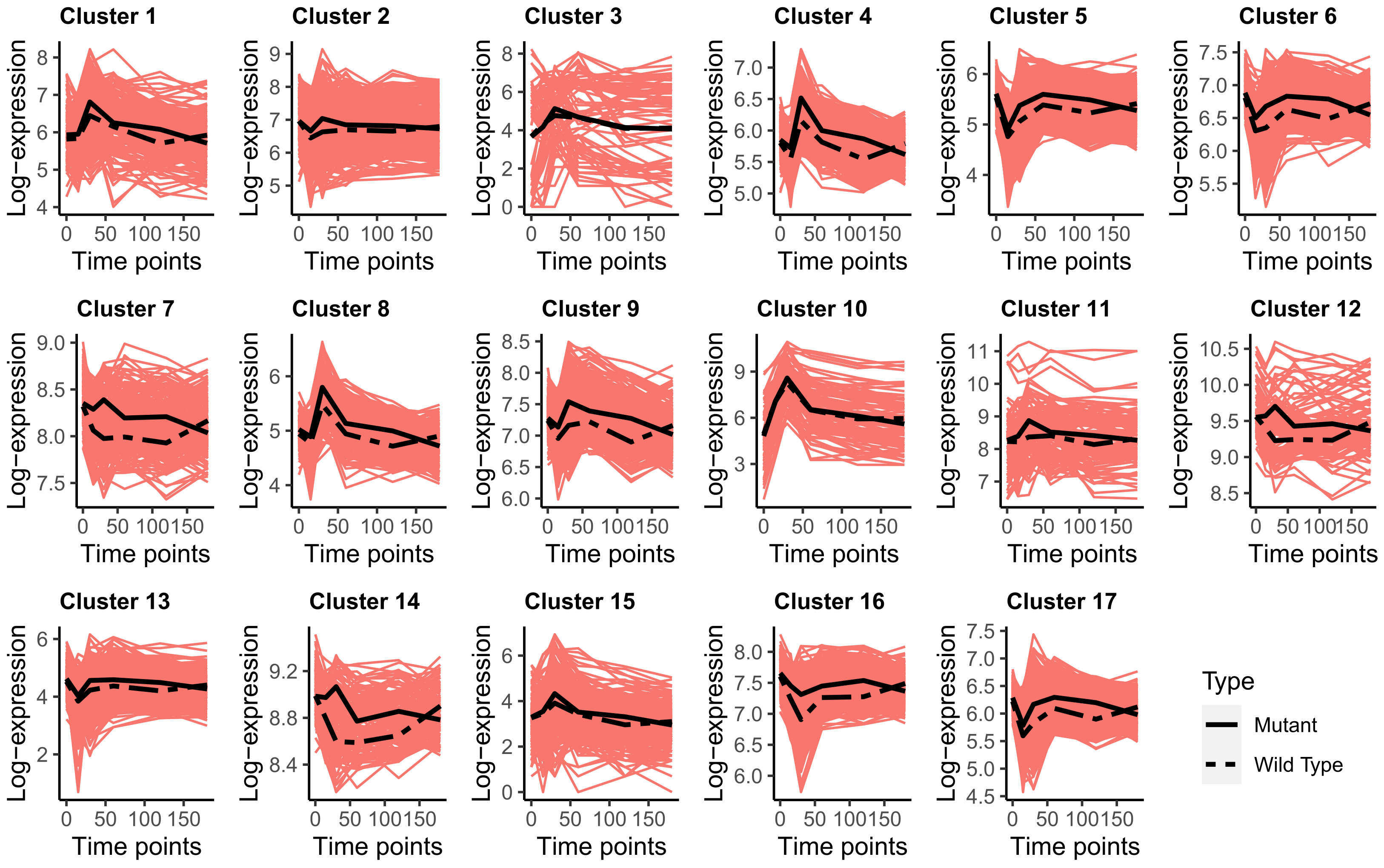
The proposed approach was used to cluster a transcriptomics dataset fission from the R package fission available through bioconductor. The dataset was originally proposed by [43]. The study consists of a time course RNA-Seq experiment of fission yeast in response to oxidative stress (1M sorbitol treatment) at 0, 15, 30, 60, 120, and 180 mins from two types of yeast: wild type and mutant type (aft21Δ strain).Thus, the measurements for each observation can be written using a matrix notation such that the two types of yeast are treated as rows (i.e., $r=2$), and the time points are treated as columns (i.e., $t=6$). We treat developmental stages as longitudinal.

For cluster analysis, we focused on the subset of the differentially expressed genes provided in the Supplementary Material by [43]. Genes were considered differentially expressed if their mean expression level differed in at least one time point relative to unstressed reference, and multiple testing correction was performed to ensure overall FDR was kept below 5%. A total of 3169 genes (out of 5957) were differentially expressed in wild type yeast, and 3044 genes were differentially expressed in the aft21Δ strain. For our analysis, we included the gene if it was differentially expressed in both wild type and aft21Δ strain; thus a total of 2476 genes were included.

All eight models were fitted to the dataset for $G=1$ to $G=20$, and the best fitting model was selected by BIC. A $G=17$ component “EVA” model with a constrained ${\mathbf{T}}_g$ (i.e., ${\mathbf{T}}_1={\mathbf{T}}_2=\dots ={\mathbf{T}}_{17}$) and unconstrained anisotropic ${\mathbf{D}}_g$ was selected. The constrained ${\mathbf{T}}_g$ suggests that the correlation structure (i.e., autoregressive relationship) among the developmental stages is the same for all groups. However, the unconstrained anisotropic ${\mathbf{D}}_g$ suggests that the variances at the developmental stages are different, and it varies from cluster to cluster. Visualization of the log-transformed expression values of the genes in each group along with its mean-expression trends is shown in Figure 1. As seen in Figure 1, the clusters have distinctive mean-expression trends.

4. Conclusions

A novel family of matrix variate Poisson log-normal mixture models was developed for clustering longitudinal transcriptomics data. This approach utilized a modified Cholesky decomposition of a component of the covariance matrices of the latent variable, and constraints were imposed on various components of this decomposition which resulted in a family of eight models. Performance of the proposed approach was illustrated using both simulated and real datasets where the proposed approach showed good clustering performance.

One of the limitations with the proposed approach is that it assumes that measurements are taken at the same fixed intervals for all observations, which can be restrictive. Some future work will focus on extending these models to allow for varying interval lengths between observations. Furthermore, time is continuous; hence, discretizing it can result in a loss of information. Some work will also focus on developing a modelling framework that models time as a continuous variable.

References

- Spellman, P.T.; Sherlock, G.; Zhang, M.Q.; Iyer, V.R.; Anders, K.; Eisen, M.B.; Brown, P.O.; Botstein, D.; Futcher, B. Comprehensive identification of cell cycle–regulated genes of the yeast Saccharomyces cerevisiae by microarray hybridization. Mol. Biol. Cell 1998, 9, 3273–3297. [Google Scholar] [CrossRef]
- Lee, C.W.; Stabile, E.; Kinnaird, T.; Shou, M.; Devaney, J.M.; Epstein, S.E.; Burnett, M.S. Temporal patterns of gene expression after acute hindlimb ischemia in mice: Insights into the genomic program for collateral vessel development. J. Am. Coll. Cardiol. 2004, 43, 474–482. [Google Scholar] [CrossRef]
- Louis, E.; Raue, U.; Yang, Y.; Jemiolo, B.; Trappe, S. Time course of proteolytic, cytokine, and myostatin gene expression after acute exercise in human skeletal muscle. J. Appl. Physiol. 2007, 103, 1744–1751. [Google Scholar] [CrossRef] [PubMed]
- Li, Y.; Li, M.; Tan, L.; Huang, S.; Zhao, L.; Tang, T.; Liu, J.; Zhao, Z. Analysis of time-course gene expression profiles of a periodontal ligament tissue model under compression. Arch. Oral Biol. 2013, 58, 511–522. [Google Scholar] [CrossRef] [PubMed]
- McLachlan, G.J.; Bean, R.W.; Peel, D. A mixture model-based approach to the clustering of microarray expression data. Bioinformatics 2002, 18, 413–422. [Google Scholar] [CrossRef]
- Inoue, L.Y.; Neira, M.; Nelson, C.; Gleave, M.; Etzioni, R. Cluster-based network model for time-course gene expression data. Biostatistics 2007, 8, 507–525. [Google Scholar] [CrossRef] [PubMed]
- McNicholas, P.D.; Murphy, T.B. Model-based clustering of longitudinal data. Can. J. Stat. 2010, 38, 153–168. [Google Scholar] [CrossRef]
- Si, Y.; Liu, P.; Li, P.; Brutnell, T.P. Model-based clustering for RNA-seq data. Bioinformatics 2014, 30, 197–205. [Google Scholar] [CrossRef]
- Rau, A.; Maugis-Rabusseau, C.; Martin-Magniette, M.L.; Celeux, G. Co-expression analysis of high-throughput transcriptome sequencing data with Poisson mixture models. Bioinformatics 2015, 31, 1420–1427. [Google Scholar] [CrossRef]
- Silva, A.; Rothstein, S.J.; McNicholas, P.D.; Subedi, S. A multivariate Poisson-log normal mixture model for clustering transcriptome sequencing data. BMC Bioinform. 2019, 20, 394. [Google Scholar] [CrossRef]
- Holmes, I.; Harris, K.; Quince, C. Dirichlet multinomial mixtures: Generative models for microbial metagenomics. PLoS ONE 2012, 7, e30126. [Google Scholar] [CrossRef] [PubMed]
- Subedi, S.; Neish, D.; Bak, S.; Feng, Z. Cluster analysis of microbiome data by using mixtures of Dirichlet–multinomial regression models. J. R. Stat. Soc. Ser. C (Appl. Stat.) 2020, 69, 1163–1187. [Google Scholar] [CrossRef]
- Lo, K.; Brinkman, R.R.; Gottardo, R. Automated gating of flow cytometry data via robust model-based clustering. Cytom. Part A J. Int. Soc. Anal. Cytol. 2008, 73, 321–332. [Google Scholar] [CrossRef] [PubMed]
- Chan, C.; Feng, F.; Ottinger, J.; Foster, D.; West, M.; Kepler, T.B. Statistical mixture modeling for cell subtype identification in flow cytometry. Cytom. Part A J. Int. Soc. Anal. Cytol. 2008, 73, 693–701. [Google Scholar] [CrossRef] [PubMed]
- Shen, R.; Mo, Q.; Schultz, N.; Seshan, V.E.; Olshen, A.B.; Huse, J.; Ladanyi, M.; Sander, C. Integrative subtype discovery in glioblastoma using iCluster. PLoS ONE 2012, 7, e35236. [Google Scholar] [CrossRef]
- Higgins, J.P.; Shinghal, R.; Gill, H.; Reese, J.H.; Terris, M.; Cohen, R.J.; Fero, M.; Pollack, J.R.; Van de Rijn, M.; Brooks, J.D. Gene expression patterns in renal cell carcinoma assessed by complementary DNA microarray. Am. J. Pathol. 2003, 162, 925–932. [Google Scholar] [CrossRef]
- Ma, X.J.; Salunga, R.; Tuggle, J.T.; Gaudet, J.; Enright, E.; McQuary, P.; Payette, T.; Pistone, M.; Stecker, K.; Zhang, B.M.; et al. Gene expression profiles of human breast cancer progression. Proc. Natl. Acad. Sci. USA 2003, 100, 5974–5979. [Google Scholar] [CrossRef]
- Haqq, C.; Nosrati, M.; Sudilovsky, D.; Crothers, J.; Khodabakhsh, D.; Pulliam, B.L.; Federman, S.; Miller III, J.R.; Allen, R.E.; Singer, M.I.; et al. The gene expression signatures of melanoma progression. Proc. Natl. Acad. Sci. USA 2005, 102, 6092–6097. [Google Scholar] [CrossRef]
- Humbert, S.; Subedi, S.; Cohn, J.; Zeng, B.; Bi, Y.M.; Chen, X.; Zhu, T.; McNicholas, P.D.; Rothstein, S.J. Genome-wide expression profiling of maize in response to individual and combined water and nitrogen stresses. BMC Genom. 2013, 14, 3. [Google Scholar] [CrossRef]
- Misyura, M.; Guevara, D.; Subedi, S.; Hudson, D.; McNicholas, P.D.; Colasanti, J.; Rothstein, S.J. Nitrogen limitation and high density responses in rice suggest a role for ethylene under high density stress. BMC Genom. 2014, 15, 681. [Google Scholar] [CrossRef]
- Wolfe, J.H. Pattern clustering by multivariate mixture analysis. Multivar. Behav. Res. 1970, 5, 329–350. [Google Scholar] [CrossRef]
- Luan, Y.; Li, H. Clustering of time-course gene expression data using a mixed-effects model with B-splines. Bioinformatics 2003, 19, 474–482. [Google Scholar] [CrossRef]
- McNicholas, P.D.; Subedi, S. Clustering gene expression time course data using mixtures of multivariate t-distributions. J. Stat. Plan. Inference 2012, 142, 1114–1127. [Google Scholar] [CrossRef]
- Coffey, N.; Hinde, J.; Holian, E. Clustering longitudinal profiles using P-splines and mixed effects models applied to time-course gene expression data. Comput. Stat. Data Anal. 2014, 71, 14–29. [Google Scholar] [CrossRef]
- Koestler, D.C.; Marsit, C.J.; Christensen, B.C.; Kelsey, K.T.; Houseman, E.A. A recursively partitioned mixture model for clustering time-course gene expression data. Transl. Cancer Res. 2014, 3, 217. [Google Scholar] [PubMed]
- Love, M.I.; Huber, W.; Anders, S. Moderated estimation of fold change and dispersion for RNA-seq data with DESeq2. Genome Biol. 2014, 15, 550. [Google Scholar] [CrossRef]
- Dong, K.; Zhao, H.; Tong, T.; Wan, X. NBLDA: Negative binomial linear discriminant analysis for RNA-Seq data. BMC Bioinform. 2016, 17, 369. [Google Scholar] [CrossRef]
- Doss, D. Definition and characterization of multivariate negative binomial distribution. J. Multivar. Anal. 1979, 9, 460–464. [Google Scholar] [CrossRef]
- Brijs, T.; Karlis, D.; Swinnen, G.; Vanhoof, K.; Wets, G.; Manchanda, P. A multivariate Poisson mixture model for marketing applications. Stat. Neerl. 2004, 58, 322–348. [Google Scholar] [CrossRef]
- Subedi, S.; Browne, R.P. A family of parsimonious mixtures of multivariate Poisson-lognormal distributions for clustering multivariate count data. Stat 2020, 9, e310. [Google Scholar] [CrossRef]
- Silva, A.; Rothstein, S.J.; McNicholas, P.D.; Subedi, S. Finite mixtures of matrix-variate Poisson-log normal distributions for three-way count data. arXiv 2018, arXiv:1807.08380. [Google Scholar] [CrossRef]
- Pourahmadi, M. Joint mean-covariance models with applications to longitudinal data: Unconstrained parameterisation. Biometrika 1999, 86, 677–690. [Google Scholar] [CrossRef]
- Dempster, A.P.; Laird, N.M.; Rubin, D.B. Maximum likelihood from incomplete data via the EM algorithm. J. R. Stat. Soc. Ser. B 1977, 39, 1–22. [Google Scholar]
- Wainwright, M.J.; Jordan, M.I. Graphical models, exponential families, and variational inference. In Foundations and Trends in Machine Learning; The Essence of Knowledge: Delft, The Netherlands, 2008; Volume 1, pp. 1–305. [Google Scholar]
- McNicholas, P.D.; Jampani, K.R.; Subedi, S. Longclust: Model-Based Clustering and Classification for Longitudinal Data; R Package Version 1.2.3; R Package: Vienna, Austria, 2019. [Google Scholar]
- Aitken, A.C. A series formula for the roots of algebraic and transcendental equations. Proc. R. Soc. Edinb. 1926, 45, 14–22. [Google Scholar] [CrossRef]
- Böhning, D.; Dietz, E.; Schaub, R.; Schlattmann, P.; Lindsay, B. The distribution of the likelihood ratio for mixtures of densities from the one-parameter exponential family. Ann. Inst. Stat. Math. 1994, 46, 373–388. [Google Scholar] [CrossRef]
- Schwarz, G. Estimating the dimension of a model. Ann. Stat. 1978, 6, 461–464. [Google Scholar] [CrossRef]
- Hubert, L.; Arabie, P. Comparing Partitions. J. Classif. 1985, 2, 193–218. [Google Scholar] [CrossRef]
- Rau, A.; Celeux, G.; Martin-Magniette, M.; Maugis-Rabusseau, C. Clustering High-Throughput Sequencing Data with Poisson Mixture Models; Technical Report RR-7786; INRIA: Saclay, France, 2011. [Google Scholar]
- Rau, A.; Celeux, G.; Martin-Magniette, M.L.; Maugis-Rabusseau, C. HTSCluster: Clustering High-Throughput Transcriptome Sequencing (HTS) Data; R Package Version 2.0.4; R Package: Vienna, Austria, 2016. [Google Scholar]
- Si, Y. MBCluster.Seq: Model-Based Clustering for RNA-Seq Data; R Package Version 1.0; R Package: Vienna, Austria, 2012. [Google Scholar]
- Leong, H.S.; Dawson, K.; Wirth, C.; Li, Y.; Connolly, Y.; Smith, D.L.; Wilkinson, C.R.; Miller, C.J. A global non-coding RNA system modulates fission yeast protein levels in response to stress. Nat. Commun. 2014, 5, 3947. [Google Scholar] [CrossRef]
Figure 1.
Visualization of the log-transformed expression values along with its mean-expression values for the two yeast types (solid black line for the mutant and dashed black line for wild type) for all 17 clusters of the transcriptomics dataset.