1. Introduction
Survival analysis is a branch of statistics widely used by the scientific community of leading areas of knowledge to study the time until the occurrence of an event of interest. The time of failure, also referred to as the event time or survival time, denotes the time at which an event of interest occurs. In medical contexts, for instance, it may indicate the time until a patient’s death, cure, or disease relapse. In engineering, this failure time can be the time until a piece of equipment or component becomes defective. In the criminal justice field, the time of failure may denote the time elapsed between a prisoner’s release and the occurrence of a subsequent crime, among other possibilities.
The principal distinction between survival analysis techniques and classical statistical methods, such as regression analysis and the design of experiments, lies in the former’s ability to incorporate information from censored data into statistical analysis. The incorporation of censored data information, which is partial observation of the response, is the main feature of survival data.
The non-parametric Kaplan–Meier estimator proposed by Kaplan [
1] is undoubtedly the most widely used in the literature to estimate survival function. However, non-parametric techniques are limited in their ability to include explanatory variables in the analysis. To address this, appropriate regression models are used for censored data, such as parametric and semi-parametric models. The Cox regression model [
2], a semi-parametric approach, offers the flexibility to incorporate time-dependent explanatory variables with ease and is more flexible compared to parametric models, as it does not assume a specific statistical distribution in survival time. However, the Cox model assumes that hazards are proportional, with the supposition that the risk of failure is proportional over time.
Although the proportional hazard assumption can be easily verified in one dimension, verification of this assumption becomes challenging when working with higher dimensions. Moreover, adjusting a Cox model can be difficult when the number of explanatory variables exceeds the number of individuals since it uses partial probability to estimate the parameters [
3]. Given the challenges of verifying the proportional hazard assumption in higher dimensions and the strong assumption inherent in the Cox model, it is necessary to employ a more flexible and high predictive performance approach, such as support vector machines (SVMs). SVMs are based on the theory of statistical learning developed by Vapnik [
4]. They are known for their good and theoretical properties and high classification accuracy in classification problems when working with large dimensions [
5].
Emerging from the use of the wavelet kernel, the wavelet kernel with the support vector machines [
6] has been shown to be quite effective in the approximation process of non-linear functions in order to obtain, in some cases, a predictive capability superior to that of the radial basis function (RBF) kernel [
7] in a wide range of applications, such as economics [
8], wind speed prediction [
9], and carbon price prediction [
10]. Examples of its use are commonly seen in conjunction with neural networks for classification problems as a way to improve the predictive capacity of the model [
11,
12,
13,
14].
This paper aims to propose a new method, namely wavelet support vector censored regression (WSVCR), and compare the Cox model with traditional support vector regression (SVR) and traditional support vector regression for censored data (SVCR) models.
Section 2 provides an overview of the survival analysis, the Cox proportional hazards model, and the C-index metric used for evaluation.
Section 3 presents a brief overview of support vector models and the proposition of WSVCR. The simulation study is presented in
Section 4. Benchmarking analysis and real biomedical data application are given in
Section 5. Finally,
Section 6 concludes the paper with the final considerations.
2. Survival Analysis
A characteristic of survival data is the presence of censorship. In the context of censored data, the time of occurrence of the event of interest may be to the right of the recorded time (“right-censoring”), or the recorded time may be greater than the failure time (“left-censoring”). The following notations are used throughout the text. The censored observation is defined as where is a p-dimensional explanatory variable vector, is the lower bound and is the upper bound. The tuple representing observation with left- and right-censoring is given by and , respectively, . If the data are uncensored, the observation is given by where is the corresponding survival time. In some situations, the indicator is used to denote whether an event is observed () or if the observation is censored ().
2.1. Cox Proportional Hazards Model
The Cox model is the most popular statistical approach to survival analysis. The basic assumption with using this model is that hazards are proportional. This assumption is reflected in the formula [
15],
where
is the hazard function for the
ith individual,
is the explanatory variable
j for individual
i,
is the slope term for the
jth explanatory variable, and
refers to a hazard function for an individual with zeros for all features. The coefficients of the Cox regression model (
’s) are obtained via maximum likelihood estimation. Violation of the assumption of proportional hazards may lead to bias in estimating the model coefficients.
2.2. C-Index
The concordance index (C-index) is a performance evaluation metric widely used in survival analysis, which can be viewed as a generalization of area under the curve for continuous response variables. It assesses a model’s performance by comparing the predicted survival time and the true survival time for pairs of observations and determining the proportion where they share the same ordering (i.e., they are concordant). Chen et al. [
16], Shivaswamy et al. [
17], Van Belle et al. [
18] and Fouodo et al. [
3] employed the C-index to evaluate the performance of the proposed survival models. In general, this measure estimates the model’s performance in the classification of the survival times and evaluates the degree of agreement between the model’s predictions or risk estimates and the observed survival outcomes.
The C-index can be defined as the probability of agreement between two randomly chosen observations, that is, the observation that has the shortest lifetime must also have the highest risk score and vice versa [
19,
20]. The C-index may be expressed as
where
is an estimate function of
, for example, the risk score estimated by the Cox model,
I is the indicator function, and
is a comparability indicator for a pair of observations
defined as
A C-index with value 1 indicates perfect agreement. On the other hand, 0.5 means a random prediction. Survival data usually yield values between 0.6 and 0.7. The performance of some analysts in the stock market has a C-index between 0.3 and 0.4.
According to Brentnall and Cuzick [
21], the C-index was used for the first time to estimate the degree to which an observation chosen at random from one distribution was superior to that chosen independently from another distribution so that it can also be understood as a generalization of the Wilcoxon–Mann–Whitney statistics [
22,
23]. In this case, the concordance index can be written as [
24]
where in the context of the order graph, which represents the ordering of survival times for two subjects in a graphical form (refer to Steck et al. [
24] for further details), the function
is defined as 1 if
, and 0 otherwise. Here,
denotes the number of edges in the graph, and
represents the model-predicted survival time for subject
i.
Considering the Cox proportional-hazards model, the C-index may be written as
where
measures the risk. Furthermore, considering the joint survival or failure time, the C-index is given by
where
represents the predicted value, that is, a shorter failure time means a lower predicted value.
3. Support Vector Regression Approach
The support vector machine, proposed by [
25], is used to create an optimal hyperplane that can separate a set of observations by maximizing the distance between the margins. Originally devised for the separation of two classes, the model can be used for linear and non-linear cases through the different kernel functions, and has become a widely used model, given its power of generalization and theoretical foundation.
3.1. Traditional Support Vector Regression
Support vector regression machines [
26] were proposed as generalized versions of support vector machines for regression tasks. Instead of creating a hyperplane with a maximum margin in feature space, support vector regression builds an optimal hypertube which considers the observations inside the hypertube as constraints, as well as minimizing the distance among the observations and the center of the hypertube.
Let a dataset be {
},
i = 1, …,
n, where
n is the number of observations,
is the response variable,
are the explanatory variables,
is the parameter vector on the hypertube as well as the hyperparameters
and
C. Vapnik [
26] showed that considering slack variables
and the optimization of convex objective function is given by
where
. Hyperparameter
C represents the regularization constant responsible for imposing weight to minimize errors. Additionally, the hypertube may be expressed in the dual form optimization given by the following Equation (
1) and its respective constraints [
26]:
This approach of SVR works successfully in linear regression problems. However, there are cases where non-linearity exists among the explaining and predictor variables. In these cases, the kernel trick may be used, based on Mercer’s theorem [
27] in order to deal with non-linearity. Using kernel methods, rather than considering the input space, higher feature spaces are considered, where the observations could be linearly separable through the function
, where
is a map function and replaces the inner product in Equation (
1). These functions are defined as semi-definite kernel functions [
28].
Many types of kernel functions are used in distinct regression examples. The choice of specific kernel functions creates unique non-linear mappings, and the efficiency of the resulting SVR usually depends on the correct choice of the kernel [
29]. There are several kernel functions in the general SVR framework, some of the most common of which are considered in this paper.
Table 1 displays these kernels for hyperparameters
and
.
The trick is precisely to find the appropriate kernel to build the model for a given set of data so that there is no single appropriate kernel function for every type of database. The decision of the most appropriate kernel function may be determined by grid search [
30], as well the choice of the best hyperparameters.
3.2. Support Vector Censored Regression
As mentioned in
Section 2, the censored observation is defined as
where
is the lower bound and
is the upper bound. In the censored data context, there exist two different censors: the data can be left-censored, with the tuple that represents that observation being given by
, and the data can be right-censored, with
. If the data are not censored, the observation is given by the tuple
.
In order to develop a model that can use all available information, even when the data are censored, Shivaswamy et al. [
17] developed the support vector censored regression (SVCR) approach. The proposal is generalized for both censoring types [
17]. However, in their work, only left-censored data were explored, as well as a few kernel functions, linear and polynomial.
In the SVCR, the loss function is defined by
Let
,
and
. Then,
is the index of uncensored samples, while
and
are the index of the samples which are right- and left-censored, respectively. Letting
and
, the optimization of the convex objective function for SVCR is given by
Expanding this formulation through the Lagrangian multipliers, the dual formulation [
26] considering the censored data becomes
With the SVCR approach, the dot product also can be replaced for the kernel function
to obtain a non-linear function mapping. Some works already demonstrated the use of the support vector regression approach to censored data only use three types of kernel functions: linear, polynomial and Gaussian [
17,
18]. This paper presents a proposition of a new SVCR, as well as presenting a comparison with other types of kernel functions in order to evaluate how the SVCR algorithm would behave for these other cases.
3.3. Wavelet Kernel in Support Vector Models
Wavelets are a tool used to decompose functions, operators, or data into various frequency components, which enables the study of each component individually. In this context, wavelet support vector machine was introduced by Zhang et al. [
6] based on the aggregation of the wavelet kernel to the support vector machine theory. The wavelet kernel is a kind of multidimensional wavelet function which approximates arbitrary non-linear functions [
31]. In this sense, the main idea behind the wavelet analysis is to approximate a function or a signal by a family of functions generated by dilations or contractions (scaling) and translations of a function called the mother wavelet.
The wavelet transformation of a function
for
may be written as
where
where
is the mother wavelet function,
A and
B,
A is a dilation factor, and
B is a translation factor.
This approximation in finite
t terms is given by
with
is the approximation of
.
The Mercer theorem gives the conditions that a dot product kernel must satisfy, and these properties are extended to the support vector regression and support vector censored regression as cited in
Section 3. The choice of the wavelet plays a crucial role in the analysis, detection, and localization of power quality disturbances. In this context, using properties of translation-invariant kernels and multidimensional wavelet functions, Zhang et al. [
6] construct a translation-invariant wavelet kernel by the following wavelet mother function:
which is the cosine–Gaussian wavelet, which is the real part of the Morlet wavelet [
32].
Wavelet support vector censored regression (SVCR) is the importation of the wavelet kernel in Equation (
2), given the optimization of the convex objective function in the dual formulation for the censored data expressed in Equation (
3) on the same constraints:
where
the denotes the
kth component of the explanatory variable of the
ith training observation.
WSVCR and SVCR were implemented in the
R software [
33], and the dual Lagrangian problem was solved using the quadratic programming approach [
34]. Additionally, in order to speed up the SVCR approach, the same algorithm can use the sequential minimal optimization (SMO) [
35] to solve faster the dual optimization problem presented in Equations (
1)–(
3).
4. Simulation Study
In order to evaluate the performance of different kernel functions used in the support vector censored regression approach to survival data, we firstly explored simulated data, for which it is possible to create a controlled environment for the experiment. The data generation model is defined over three explanatory variables and , which follow the distributions below:
;
;
.
To capture the time behavior from observations in survival data analysis, we use the Weibull distribution to generate the time of each observation since several works already demonstrated that it is appropriate to generate this kind of data [
36,
37,
38]. The time generation is given by
, where the scale parameter and shape parameter are given by
respectively. Equation (
4) was proposed in order to represent non-linear behavior among explanatory variables. In this case, the simulation of this artificial dataset is based on varying sample sizes and proportions of censored observations, along with a non-linear relationship between the explanatory variables and the true generation function. This approach is necessary, as most traditional survival approaches fail to meet these assumptions as the case Cox model, which assumes hazard proportionality. For this reason, SVR or SVCR models can handle with this non-linear relationship, and our focus is on studying these models using the wavelet kernel in comparison with the other common kernels.
The setting of a simulated dataset was generated, varying
and the ratio of censored observations
. To evaluate the results among the different approaches, the C-index was used. The measures were calculated over a repeated holdout validation with 100 repetitions and a split ratio of 70–30% of training–test, respectively [
39,
40]. Additionally, the tuning process on SVR and SVCR was realized through a grid search, varying the parameters
,
and
A. The results are summarized by mean in
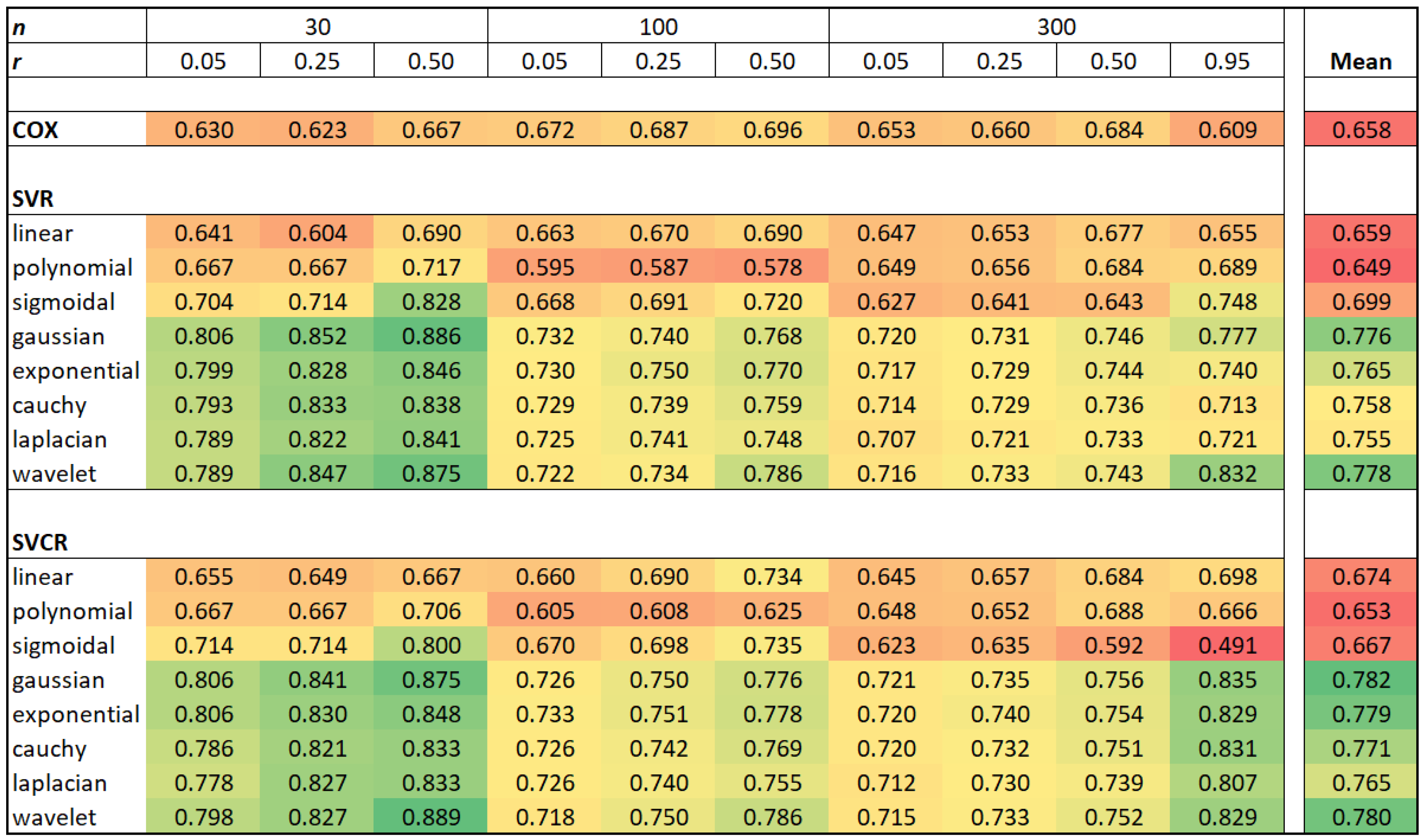
Table 2, where the bold values identify the best concordance index for each scenario. The results summarize about 673,200 fitted models over 1200 Monte Carlo samples. In the
Appendix A, a more detailed summary is provided by median, minimum, maximum and standard deviation. The results corroborate with the outperforming of wavelet SVCR in the centrality and the dispersion of the best concordance.
Table 2 displays that the wavelet SVCR generally outperforms the other methods, considering the C-index. Additionally, the SVCR with other kernels functions still greater than the traditional Cox model, which is similar to SVR with the linear kernel.
5. Real Data Applications
5.1. Benchmarking Data
In addition to the evaluation of the SVCR using simulated data, its performance with various kernel functions was also assessed on real data benchmarks that are featured in several survival analysis publications [
17,
41]. There are a total of seven datasets, each with a distinct number of observations, explanatory variables, and ratio of censored instances.
Table 3 displays the general statistics of the datasets, where
n is the sample size,
p the number of input variables and
r the censuring rate. This was done to increase diversity among the datasets on which the models were built. To determine the best model, the C-index was selected as the primary parameter, where a larger C-index indicates a better model.The parameters used in the grid search for the tuning process were the same in the simulation—
and
—based on the C-index maximization. The validation technique was also the same: repeated holdout with 30 repetitions and a split ratio of 70–30%.
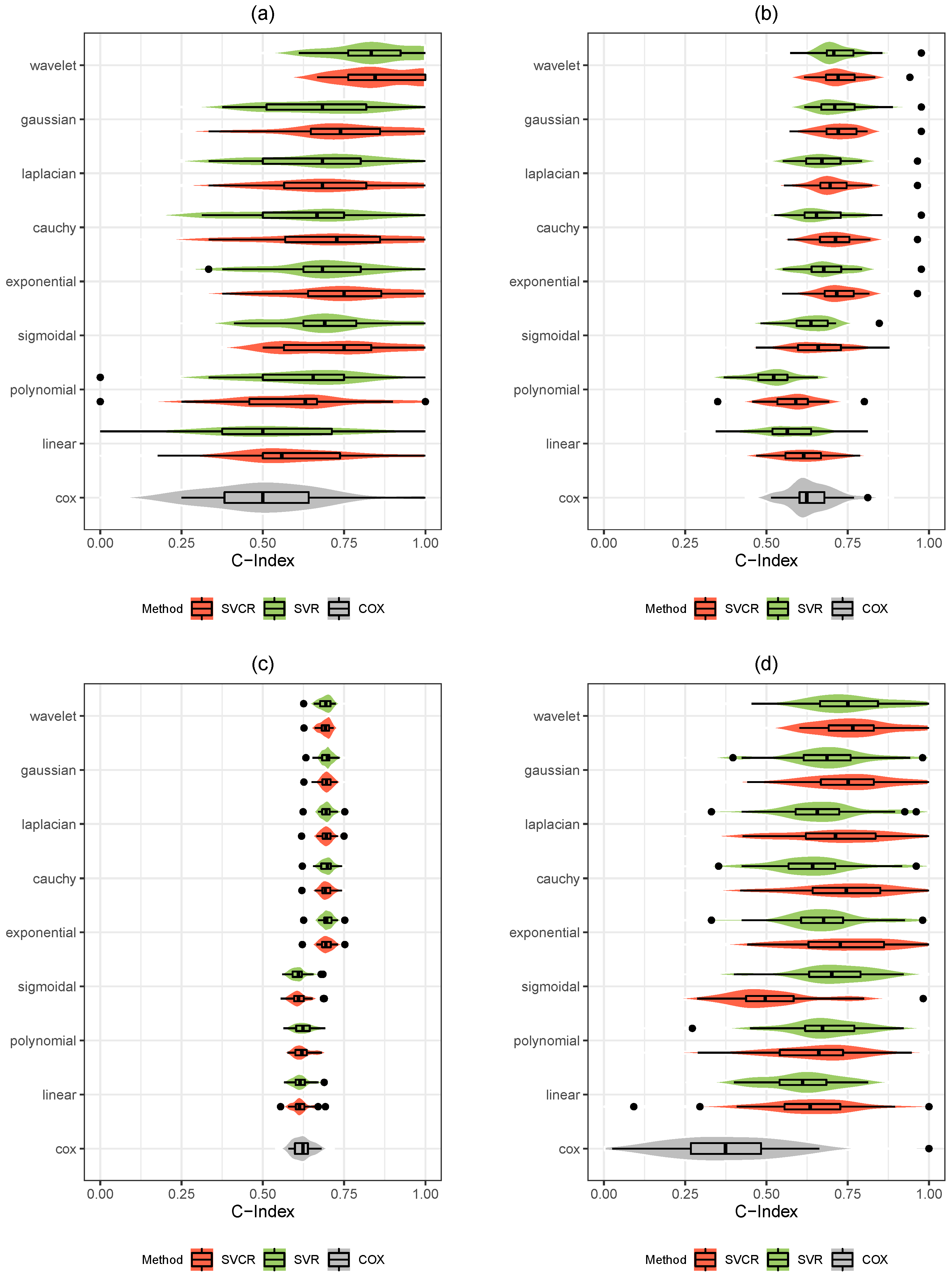
The result is summarized in
Table 4, which presents the mean C-index over the 30 holdout samples. The maximum C-index values for each dataset are shown in bold values.
The results presented in
Table 4 emphasize the great efficiency of the SVCR method. It is evident that this approach outperforms both the SVR and Cox models. It is important to notice that the wavelet kernel was the best-performing kernel function, with the largest value in 4 out of 7 in the benchmark dataset. Additionally, 70% of kernel functions that achieved the best result were among the most commonly used kernel functions in studies employing the SVCR method, i.e., linear, polynomial, and Gaussian. Therefore, the results indicate the importance of carefully selecting the correct kernel function since the exponential, Cauchy and Laplacian kernels produced the highest C-index in most cases.
The result is also summarized in
Figure 1, which schematically plots the C-index for all datasets to confirm the superiority of the SVCR approach compared with other models.
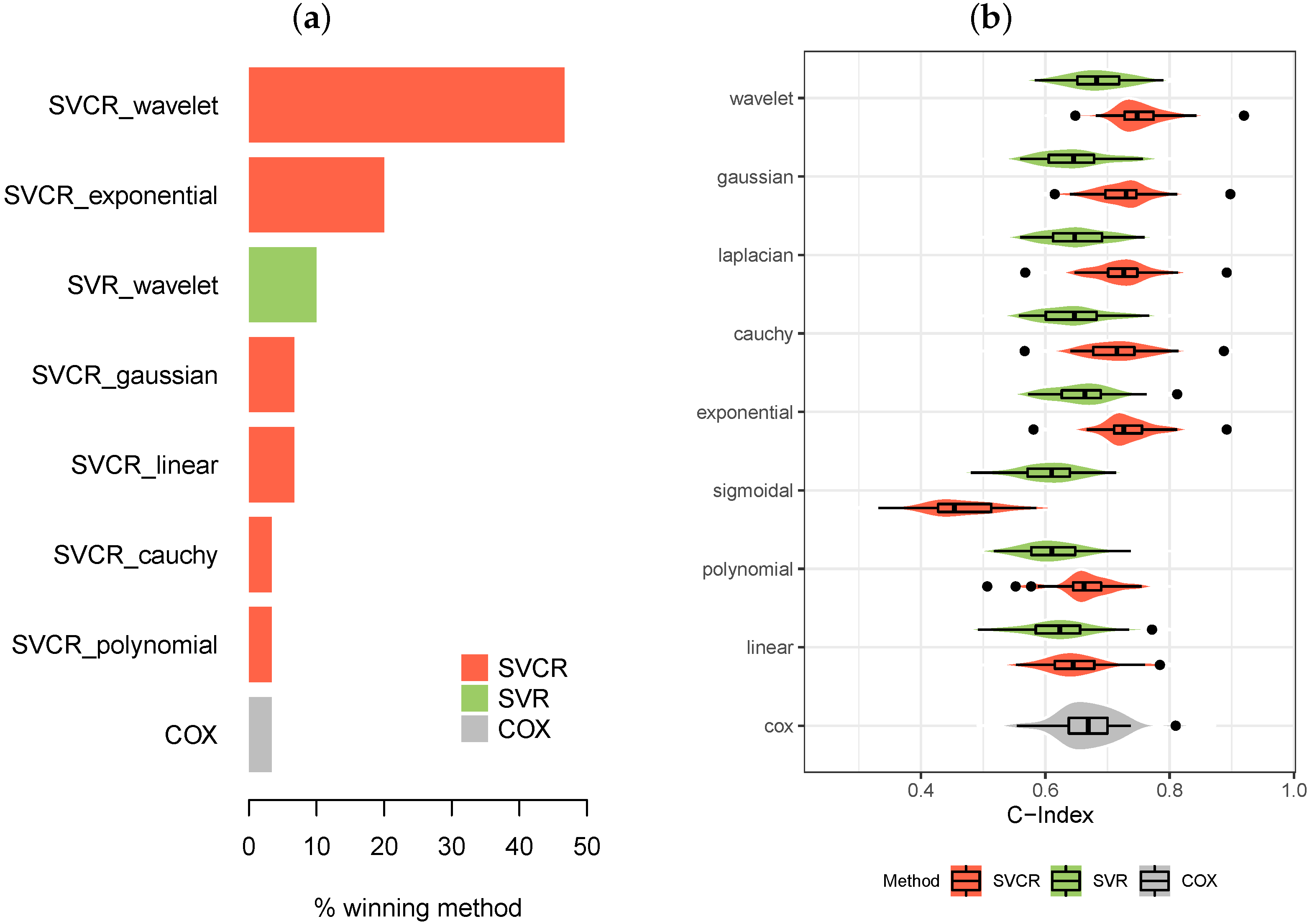
Figure 2, in turn, shows the rate of times each model was considered the winner over the 30 repetitions performed during the experiments. In this way, it is possible to observe, once again, the superiority of the wavelet kernel over the other kernels, either for the pure SVR approach, or mainly for the SVCR approach.
5.2. Biomedical Real Data
The dataset is based on research conducted by the Heart Institute at the “das Clínicas” Hospital, Faculty of Medicine, Universidade de São Paulo, Brazil (
https://www.hc.fm.usp.br, accessed on 18 Janary 2023), with the purpose of comparing the length of stay for heart disease patients undergoing cardiac surgery [
42]. This study considered 145 patients and 7 variables, of which 5 are the explanatory variables, as well as the response variable and the censoring indicator. The data were recently analyzed by [
43], using the Weibull regression model and the random survival forest (RSF) model.
The response variable, T, represents the amount of time (in hours) from the patient’s admission to their discharge from the surgical ward and is accompanied by an indicator variable, . If , there is censoring, meaning the exact length of stay is unknown. If is non-zero, the length of stay is known exactly. Additionally, the following explanatory variables were taken into account: the age of the patient in years (), the type of protocol (), which can be either conventional (0) or fast track (1), race (), which is divided in the Brazilian classification into white (1), black (2), and yellow (3), sex (), which is divided between female (0) and male (1), and the type of patient (), separated into congenital (0) and coronary (1).
Table 5 presents the descriptions of some of these variables along with their corresponding descriptive statistics. It was observed that for patients with congenital heart disease who were monitored under the traditional protocol, their age ranged from 0.3 to 49 years, while for those under the fast-track protocol, their age ranged from 0.8 to 38 years. For patients with coronary heart disease who were monitored under the traditional protocol, their age ranged from 18 to 81 years, and for those under the fast-track protocol, their age ranged from 38 to 79 years. The censuring rate (
r) for these data is 0.041.
The parameters used in the grid-search for the tuning process were similar to previous applications varying the parameters
,
and
A. The concordance was investigated by repeated holdout validation with 100 repetitions and a split ratio of 70–30% of training–test, respectively.
Figure 3 displays the grid search results of the wavelet SVCR for the 36 different possibilities, where it is observed that the highest values of C-index are obtained by increasing the values of
A.
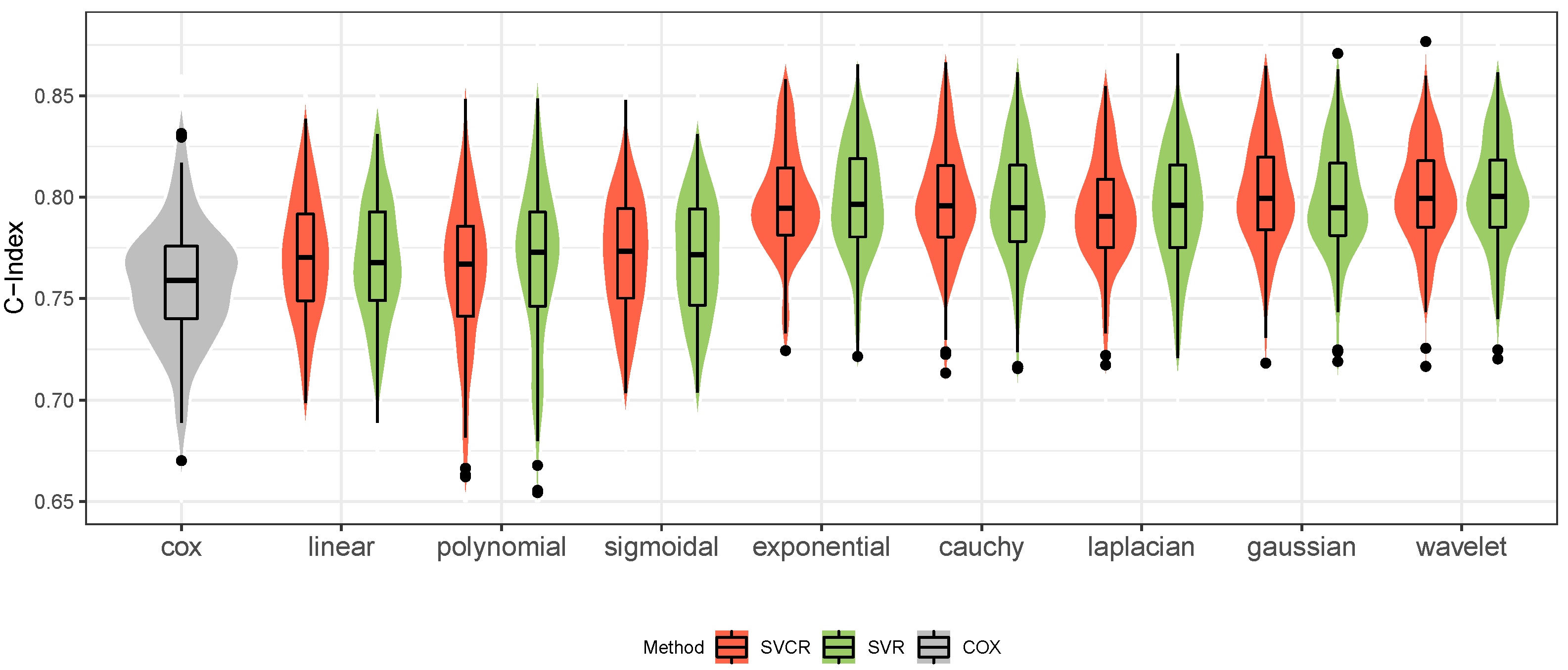
Table 6 presents the average values obtained from 100 repetitions, revealing the superior performance of the wavelet kernel for both SVR and SVCR approaches. Notably, the results show less variation in the wavelet kernel across tests with the SVR approach, which is expected due to the low censuring rate. This trend is further illustrated in
Figure 4, where the wavelet and Gaussian kernel models exhibit the best performance.
6. Final Comments
This paper proposes the WSVRC approach and compares different methods and kernel functions applied to survival data. Three different approaches are discussed: (i) the standard survival analysis approach, i.e., the Cox proportional hazards model; (ii) the support vector machine approach for regression models, i.e., the SVR; and (iii) the support vector approach for censored data, i.e., the SVCR, with the novel WSVCR model. The simulation results and applications show that the WSVCR approach is either equivalent to or outperforms the other methods. Hence, it is not advisable to persist with a model that requires a strong assumption to be validated. Instead, the WSVCR approach, which is more flexible and general, may be employed.
Furthermore, this article presents an extensive study on different kernel functions and demonstrates that kernels such as exponential, cauchy, and Laplacian show good performance and are not often considered in many papers, as most of them only employ the most common kernels (i.e., linear, polynomial, and Gaussian).
Author Contributions
Conceptualization, A.A.; methodology, A.A. and M.M.; software, M.M., J.S.P. and A.A.; validation, A.A. and R.O.; investigation, M.M., R.O. and A.A.; data curation, M.M. and J.S.P.; writing—original draft preparation, M.M. and J.S.P.; writing—review and editing, M.M., A.A. and R.O.; supervision, A.A. All authors have read and agreed to the published version of the manuscript.
Funding
This research was partially supported by the National Council for Scientific and Technological Development (CNPq) through the grant 305305/2019-0 (R.O.), Comissão de Aperfeiçoa-mento de Pessoal do Nível Superior (CAPES), from the Brazilian government and Science Foundation Ireland Career Development Award grant number 17/CDA/4695 and SFI research centre award 12/RC/2289P2 (M.M.).
Institutional Review Board Statement
Not applicable.
Informed Consent Statement
Not applicable.
Data Availability Statement
Not applicable.
Conflicts of Interest
The authors declare no conflict of interest.
Appendix A
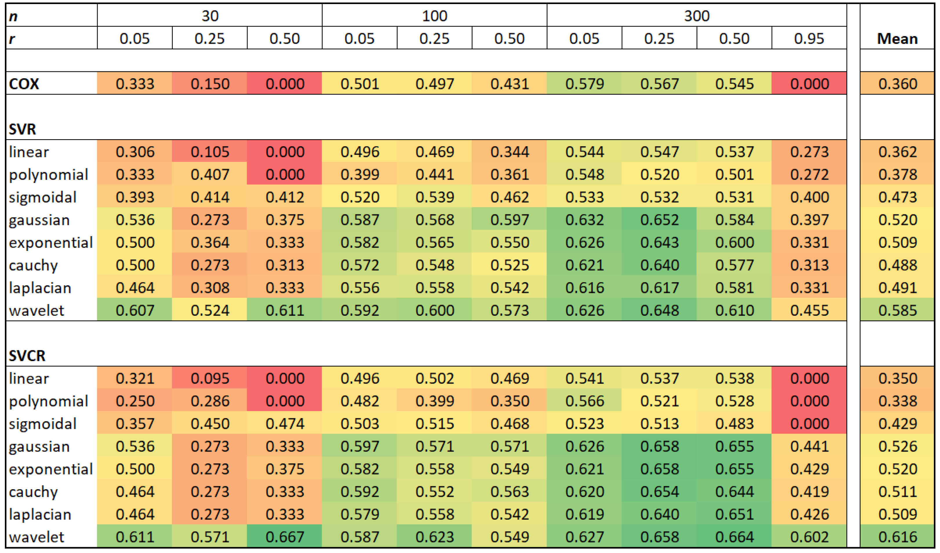
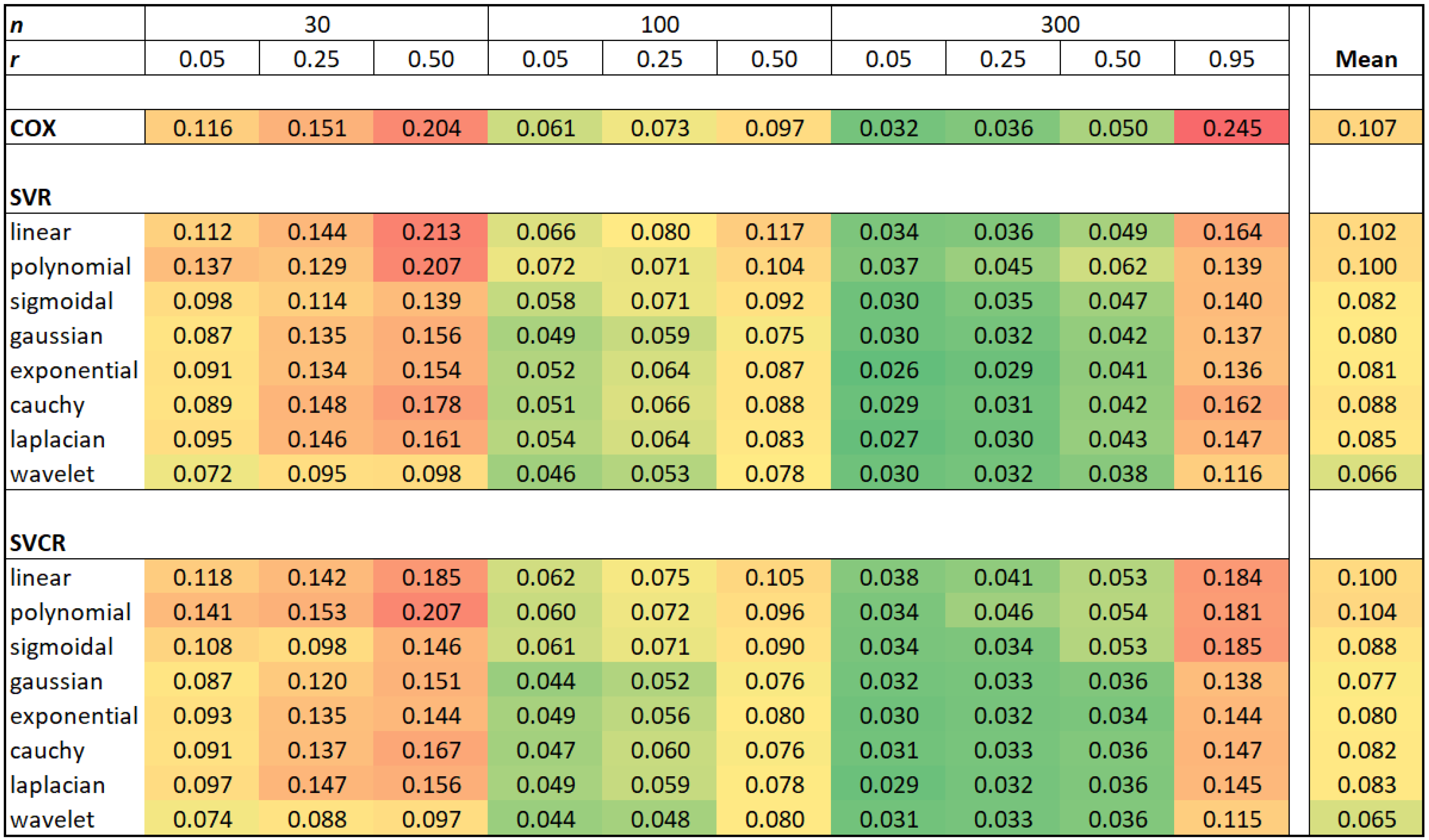
This Appendix refers to more general summary of the simulation results displayed in
Section 4. The
Figure A1,
Figure A2,
Figure A3 and
Figure A4 are related to the median, minimum, maximum and standard deviation over the 100 holdout repetitions. The values are showed in traffic light scale.
Figure A1.
Median of C-index distribution in the simulation study.
Figure A1.
Median of C-index distribution in the simulation study.
Figure A2.
Minimum of C-index distribution in the simulation study.
Figure A2.
Minimum of C-index distribution in the simulation study.
Figure A3.
Maximum of C-index distribution in the simulation study.
Figure A3.
Maximum of C-index distribution in the simulation study.
Figure A4.
Standard deviation of C-index distribution in the simulation study.
Figure A4.
Standard deviation of C-index distribution in the simulation study.
References
- Kaplan, E.L.; Meier, P. Nonparametric Estimation from Incomplete Observations. J. Am. Stat. Assoc. 1958, 53, 457–481. [Google Scholar] [CrossRef]
- Cox, D.R. Regression Models and Life-Tables. J. R. Stat. Soc. 1972, 34, 187–220. [Google Scholar] [CrossRef]
- Fouodo, C.J.; König, I.R.; Weihs, C.; Ziegler, A.; Wright, M.N. Support Vector Machines for Survival Analysis with R. R J. 2018, 10, 412–423. [Google Scholar] [CrossRef]
- Vapnik, V.N. The Nature of Statistical Learning Theory; Springer: Berlin/Heidelberg, Germany, 1995; pp. 412–414. [Google Scholar]
- Cervantes, J.; Li, X.; Yu, W.; Li, K. Support vector machine classification for large data sets via minimum enclosing ball clustering. Neurocomputing 2008, 71, 611–619. [Google Scholar] [CrossRef]
- Zhang, L.; Zhou, W.; Jiao, L. Wavelet support vector machine. IEEE Trans. Syst. Man Cybern. Part (Cybernetics) 2004, 34, 34–39. [Google Scholar] [CrossRef]
- Van, M.; Hoang, D.T.; Kang, H.J. Bearing fault diagnosis using a particle swarm optimization-least squares wavelet support vector machine classifier. Sensors 2020, 20, 3422. [Google Scholar] [CrossRef]
- Fan, Y.; Sun, Z. CPI big data prediction based on wavelet twin support vector machine. Int. J. Pattern Recognit. Artif. Intell. 2021, 35, 2159013. [Google Scholar] [CrossRef]
- Hazarika, B.B.; Gupta, D.; Natarajan, N. Wavelet kernel least square twin support vector regression for wind speed prediction. Environ. Sci. Pollut. Res. 2022, 22, 86320–86336. [Google Scholar] [CrossRef]
- Sun, W.; Xu, C. Carbon price prediction based on modified wavelet least square support vector machine. Sci. Total Environ. 2021, 754, 142052. [Google Scholar] [CrossRef]
- Yahia, S.; Said, S.; Zaied, M. Wavelet extreme learning machine and deep learning for data classification. Neurocomputing 2022, 470, 280–289. [Google Scholar] [CrossRef]
- Mo, Z.; Zhang, Z.; Tsui, K.L. The variational kernel-based 1-D convolutional neural network for machinery fault diagnosis. IEEE Trans. Instrum. Meas. 2021, 70, 1–10. [Google Scholar] [CrossRef]
- Szu, H.H.; Telfer, B.A.; Kadambe, S.L. Neural network adaptive wavelets for signal representation and classification. Opt. Eng. 1992, 31, 1907–1916. [Google Scholar] [CrossRef]
- Liu, J.W.; Zuo, F.L.; Guo, Y.X.; Li, T.Y.; Chen, J.M. Research on improved wavelet convolutional wavelet neural networks. Appl. Intell. 2021, 51, 4106–4126. [Google Scholar] [CrossRef]
- Zubek, V.B.; Khan, F.M. Support Vector Regression for Censored Data (SVRc): A Vovel Tool for Survival Analysis. In Proceedings of the 2008 Eighth IEEE International Conference on Data Mining, Pisa, Italy, 15–19 December 2008; Volume 1. [Google Scholar]
- Chen, Y.; Jia, Z.; Mercola, D.; Xie, X. A gradient boosting algorithm for survival analysis via direct optimization of concordance index. Comput. Math. Methods Med. 2013, 2013, 873595. [Google Scholar] [CrossRef]
- Shivaswamy, P.K.; Chu, W.; Jansche, M. A support vector approach to censored targets. In Proceedings of the Seventh IEEE International Conference on Data Mining (ICDM 2007), Omaha, NE, USA, 28–31 October 2007; pp. 655–660. [Google Scholar]
- Van Belle, V.; Pelckmans, K.; Van Huffel, S.; Suykens, J.A. Support vector methods for survival analysis: A comparison between ranking and regression approaches. Artif. Intell. Med. 2011, 53, 107–118. [Google Scholar] [CrossRef]
- Therneau, T.M.; Lumley, T. Package ‘survival’. R Top. Doc. 2015, 128, 28–33. [Google Scholar]
- Wang, J.; Williams, M.; Karafili, E. Apply Machine Learning Approaches to Survival Data; Imperial College: London, UK, 2018. [Google Scholar]
- Brentnall, A.R.; Cuzick, J. Use of the concordance index for predictors of censored survival data. Stat. Methods Med. Res. 2018, 27, 2359–2373. [Google Scholar] [CrossRef]
- Mann, H.B.; Whitney, D.R. On a test of whether one of two random variables is stochastically larger than the other. Ann. Math. Stat. 1947, 18, 50–60. [Google Scholar] [CrossRef]
- Wilcoxon, F. Probability tables for individual comparisons by ranking methods. Biometrics 1947, 3, 119–122. [Google Scholar] [CrossRef]
- Steck, H.; Krishnapuram, B.; Dehing-Oberije, C.; Lambin, P.; Raykar, V.C. On ranking in survival analysis: Bounds on the concordance index. Adv. Neural Inf. Process. Syst. 2007, 20. [Google Scholar]
- Cortes, C.; Vapnik, V. Support-vector networks. Mach. Learn. 1995, 20, 273–297. [Google Scholar] [CrossRef]
- Drucker, H.; Burges, C.J.; Kaufman, L.; Smola, A.J.; Vapnik, V. Support vector regression machines. Adv. Neural Inf. Process. Syst. 1997, 28, 155–161. [Google Scholar]
- Zanaty, E.; Afifi, A. Support vector machines (SVMs) with universal kernels. Appl. Artif. Intell. 2011, 25, 575–589. [Google Scholar] [CrossRef]
- Courant, R.; Hilbert, D. Methods of Mathematical Physics; Interscience Publ. Inc.: New York, NY, USA, 1953; Volume 1, p. 106. [Google Scholar]
- Jebara, T. Multi-task feature and kernel selection for SVMs. In Proceedings of the Twenty-First International Conference on Machine Learning, Banff, AL, Canada, 4–8 July 2004; p. 55. [Google Scholar]
- Chapelle, O.; Vapnik, V. Model selection for support vector machines. In Proceedings of the Advances in Neural Information Processing Systems, Denver, CO, USA, 29 November–4 December 1999; pp. 230–236. [Google Scholar]
- Yger, F.; Rakotomamonjy, A. Wavelet kernel learning. Pattern Recognit. 2011, 44, 2614–2629. [Google Scholar] [CrossRef]
- Gholizadeh, S.; Salajegheh, E.; Torkzadeh, P. Structural optimization with frequency constraints by genetic algorithm using wavelet radial basis function neural network. J. Sound Vib. 2008, 312, 316–331. [Google Scholar] [CrossRef]
- R Core Team. R: A Language and Environment for Statistical Computing; R Foundation for Statistical Computing: Vienna, Austria, 2020. [Google Scholar]
- Frank, M.; Wolfe, P. An algorithm for quadratic programming. Nav. Res. Logist. Q. 1956, 3, 95–110. [Google Scholar] [CrossRef]
- Platt, J. Sequential Minimal Optimization: A fast Algorithm for Training Support Vector Machines. Adv. Kernel-Methods-Support Vector Learn. 1998, 208. [Google Scholar]
- Bender, R.; Augustin, T.; Blettner, M. Generating survival times to simulate Cox proportional hazards models. Stat. Med. 2005, 24, 1713–1723. [Google Scholar] [CrossRef]
- Carroll, K.J. On the use and utility of the Weibull model in the analysis of survival data. Control Clin. Trials 2003, 24, 682–701. [Google Scholar] [CrossRef]
- Crowther, M.J.; Lambert, P.C. Simulating biologically plausible complex survival data. Stat. Med. 2013, 32, 4118–4134. [Google Scholar] [CrossRef]
- Tantithamthavorn, C.; McIntosh, S.; Hassan, A.E.; Matsumoto, K. An empirical comparison of model validation techniques for defect prediction models. IEEE Trans. Softw. Eng. 2016, 43, 1–18. [Google Scholar] [CrossRef]
- Louzada, F.; Ara, A.; Fernandes, G.B. Classification methods applied to credit scoring: Systematic review and overall comparison. Surv. Oper. Res. Manag. Sci. 2016, 21, 117–134. [Google Scholar] [CrossRef]
- Cawley, G.C.; Talbot, N.L.; Janacek, G.J.; Peck, M.W. Sparse bayesian kernel survival analysis for modeling the growth domain of microbial pathogens. IEEE Trans. Neural Netw. 2006, 17, 471–481. [Google Scholar] [CrossRef] [PubMed]
- Fernandes, A.M.d.S.; Mansur, A.J.; Canêo, L.F.; Lourenço, D.D.; Piccioni, M.A.; Franchi, S.M.; Afiune, C.M.C.; Gadioli, J.W.; Oliveira, S.d.A.; Ramires, J.A.F. Redução do período de internação e de despesas no atendimento de portadores de cardiopatias congênitas submetidos à intervenção cirúrgica cardíaca no protocolo da via rápida. Arq. Bras. Cardiol. 2004, 83, 18–26. [Google Scholar] [CrossRef] [PubMed]
- Cavalcante, T.; Ospina, R.; Leiva, V.; Cabezas, X.; Martin-Barreiro, C. Weibull Regression and Machine Learning Survival Models: Methodology, Comparison, and Application to Biomedical Data Related to Cardiac Surgery. Biology 2023, 12, 442. [Google Scholar] [CrossRef] [PubMed]
| Disclaimer/Publisher’s Note: The statements, opinions and data contained in all publications are solely those of the individual author(s) and contributor(s) and not of MDPI and/or the editor(s). MDPI and/or the editor(s) disclaim responsibility for any injury to people or property resulting from any ideas, methods, instructions or products referred to in the content. |
© 2023 by the authors. Licensee MDPI, Basel, Switzerland. This article is an open access article distributed under the terms and conditions of the Creative Commons Attribution (CC BY) license (https://creativecommons.org/licenses/by/4.0/).


