Image Segmentation of the Sudd Wetlands in South Sudan for Environmental Analytics by GRASS GIS Scripts

Abstract

This paper presents the object detection algorithms GRASS GIS applied for Landsat 8-9 OLI/TIRS data. The study area includes the Sudd wetlands located in South Sudan. This study describes a programming method for the automated processing of satellite images for environmental analytics, applying the scripting algorithms of GRASS GIS. This study documents how the land cover changed and developed over time in South Sudan with varying climate and environmental settings, indicating the variations in landscape patterns. A set of modules was used to process satellite images by scripting language. It streamlines the geospatial processing tasks. The functionality of the modules of GRASS GIS to image processing is called within scripts as subprocesses which automate operations. The cutting-edge tools of GRASS GIS present a cost-effective solution to remote sensing data modelling and analysis. This is based on the discrimination of the spectral reflectance of pixels on the raster scenes. Scripting algorithms of remote sensing data processing based on the GRASS GIS syntax are run from the terminal, enabling to pass commands to the module. This ensures the automation and high speed of image processing. The algorithm challenge is that landscape patterns differ substantially, and there are nonlinear dynamics in land cover types due to environmental factors and climate effects. Time series analysis of several multispectral images demonstrated changes in land cover types over the study area of the Sudd, South Sudan affected by environmental degradation of landscapes. The map is generated for each Landsat image from 2015 to 2023 using 481 maximum-likelihood discriminant analysis approaches of classification. The methodology includes image segmentation by ‘i.segment’ module, image clustering and classification by ‘i.cluster’ and ‘i.maxlike’ modules, accuracy assessment by ‘r.kappa’ module, and computing NDVI and cartographic mapping implemented using GRASS GIS. The benefits of object detection techniques for image analysis are demonstrated with the reported effects of various threshold levels of segmentation. The segmentation was performed 371 times with 90% of the threshold and minsize = 5; the process was converged in 37 to 41 iterations. The following segments are defined for images: 4515 for 2015, 4813 for 2016, 4114 for 2017, 5090 for 2018, 6021 for 2019, 3187 for 2020, 2445 for 2022, and 5181 for 2023. The percent convergence is 98% for the processed images. Detecting variations in land cover patterns is possible using spaceborne datasets and advanced applications of scripting algorithms. The implications of cartographic approach for environmental landscape analysis are discussed. The algorithm for image processing is based on a set of GRASS GIS wrapper functions for automated image classification.

1. Introduction

1.1. Background

Automatic segmentation is one of the important tasks required in environmental analytics and satellite image processing for pattern recognition. The Sudd is the largest wetland area in the world and the largest swamp area in the Nile Basin. The effects from hydrological, climate, and anthropogenic factors results in annual flooding of the Sudd, which yearly varies in extent and intensity. At the same time, the Sudd marshes provide key water and food resources for populations and habitats for species. A script-based framework of image processing is presented the GRASS GIS for monitoring the Sudd swamps using a time series of nine Landsat images from 2015 to 2023. The GRASS GIS techniques are successfully employed to detect changes in inundated areas of the Sudd wetlands during the last nine years to contribute to the environmental monitoring of East Africa, South Sudan (Figure 1).

A satellite image is far from being a random configuration of pixels. Rather, it exhibits a high degree of organisation, e.g., reflected in its spatial and spectral properties, such as geometric shapes of land cover types, various levels of brightness, and texture of patterns. In this regard, one of the main tasks in satellite image processing is the detection of image structures, such as polygons and groups of pixels, which form a fundamental matrix of images [1]. The most widely accepted approach to this task is image segmentation, which partitions the image into several segments representing distinct regions based on the characteristics of the pixels constituting the image. The algorithms of image partition divide a whole image into multiple segments, with a general aim to discriminate relevant and important parts of the image from the entire array of pixels on the image [2,3,4].

1.2. Current Research Status

New scripting languages present more powerful approaches to remote sensing data processing, providing a cost-effective alternative to the state-of-the-art image processing software. In this work, we present a set of scripting algorithms through the Geographic Resources Analysis Support System (GRASS) GIS to satellite image processing. The biggest algorithmic challenge we face when putting the idea of script-based image processing into practice is pattern recognition, which is also the reason why the GRASS GIS concept was undertaken in this study. This paper builds on and extends our previous research on satellite image processing using scripting algorithms [5,6].

In contrast to the previously used Python and R tools, the GRASS GIS presents a more powerful toolset for image processing. Hence, after a first look at the data quality in the RGB image scenes, one may be tempted to not even try to interpret the land cover patterns due to the high similarity of the individual patches. However, in this paper, we show that an appropriate combination of the GRASS GIS modules, image enhancement, clustering, classification, and interpretation enables us to differentiate the land cover types through recognition of patches on the images taken at different time periods.

Satellite image segmentation have received significant attention in recent years. Models developed for it have been used in numerous applications, such as surficial materials mapping [7], machine-learning-based computer vision [8], change detection threshold techniques [9], contextual pattern recognition for object detection [10,11,12], statistical segmentation [13,14], fusion detection with spectral and thermal feature combination [15], and texture synthesis [16], among many others. The segmentation of a satellite images is based on probabilistic modelling, which is applicable to a wide range of image structures [17].

Nevertheless, much software for image processing is distributed on a commercial basis. In order to reduce the cost and increase the effectiveness of image processing, a lot of approaches are proposed as an alternative to proprietary software for image processing, some of them using programming and scripting methods and some of them using embedded algorithms and libraries. Alternative ways of image processing may be used as components of workflow in various approaches to image analysis, to enhance image quality, and to adjust bands of satellite channels for specific landscape types. At the same time, various software has different mechanisms and algorithms of image processing, controlling the techniques of raster data processing. Therefore, understanding the workflow and way of image processing, the effects of specific libraries, and their performance during scripting is of great importance.

Through detecting objects and boundaries, segmentation supplies essential information for detecting relevant landscape patches of Earth visible on spaceborne images at various scales [18]. The essential part of the segmentation algorithm consists in the partition of images using thresholds, which analyses the natural image and seeks to divide the image into the regions of interest and other parts through analysis of the properties of pixels characterising land cover types in the landscapes. Various modifications of threshold algorithms exist that aim to optimise the process. Examples include, for instance, multilevel thresholding [19,20,21], double threshold approaches for two-dimensional Otsu image segmentation [22,23], weighted threshold algorithms using thread segmentation [24], and mean-shift clustering algorithms [25], to mention a few.

Specifically for remote sensing applications, segmentation recognises objects through grouping pixels with similar values of spectral reflectance identified as threshold values into unique segments on the image [26]. Threshold algorithms present an efficient method of image partition, which employs machine vision to derive the parameters of pixels discriminating the region of interest on the image from the background using properties of cells [27]. The extended approach of multilevel thresholding divides the image into multiple regions based on the level of colour intensity defined for each segment [28,29,30].

1.3. Examples of Tools and Software

Relevant examples of satellite image processing show that segmentation applied to environmental mapping gives rise to a semantically meaningful detection of vegetation assemblages, which are equivalent to habitats [31]. Selected previous works on satellite image segmentation include various developed algorithms, e.g., discriminating the regions against neighbours by semantic approach and normalisation using deep features in network convergence [32], contrasting land categories using diversity in pixels and smoothing shapes of the regions [33], iterative mean-shift clustering optimisation [34], layering images and segmenting through the R-Convolutional Neural Networks (CNNs) [35], evaluating the saliency in pixels using weighted dissimilarities in patches [36], and extracting contours by simplification [37,38].

Intuitively, using the patchy texture of images enables the detection of homogenous habitats for use in various image processing and computer vision applications in environmental analyses. The advantage of employing segmentation approaches in remote sensing data analysis is that the results are based on feature extraction independent of the choice of parametrisation of segments. A wide range of satellite image segmentations have also been reported, with case studies including the detection of shorelines [39], burned areas [40,41], or forest variables [42] and change detection in wetlands [43]. If a trackable parametrisation exists, similar to image classification, then it can be used directly with no loss of information in segmentation [44]. In such cases, the strategy of object detection in segmentation algorithms is based on the identification of the regions on the image which present an assembly of contiguous pixels that meet threshold criteria [45,46].

Conventional spectral clustering techniques have revealed critical links between polygonal approximation and the definition of the segments in image partition. This is achieved using the embedded segmentation algorithms [47,48,49]. More complex cases reduce the level of the fragmentation through contouring segment carcasses derived from the upscaled colour texture features and adjusted to the level of fragmentation [50]. In this way, colour features perform better in the classification tasks, since the region is formed by an optimised size of clusters forming segments of pixels that depict their major contour and colours [51]. Such similarity between the segments and separated objects can further be used to convert the bitmap image into segments. Other algorithms include image filtering, which can be performed through the similarity of pixels analysed by Euclidean and Mahalanobis distances, as well as segmentation that splits the image into several clusters on the scene [52,53,54].

The success of image processing can be evaluated through measured characteristics of the land cover classes which indicate changes in landscapes over time. The traditional methods of evaluation land cover types include the classification of scenes and detecting diverse landscape types using image analysis. Such an approach provides direct information on variations in land cover types and landscape dynamics due to the relationship between spectral brightness and the properties of land cover types. As a general rule, the combination of various Landsat bands enables to detect various land cover types, along with the increased wetness or dryness of soil, which indicates the content of water and may point to the desertification of landscapes or, on the contrary, increases in swamp marshes.

1.4. Research Goals and Gaps

A major advantage of the machine learning approach to remote sensing applications and computer vision is that it allows optimised modelling through algorithms of automatic image processing [55,56,57,58]. Thus, specifically for image segmentation, machine learning proposes embedded techniques of image discrimination to find the contours of the objects [59,60,61]. However, the general workflow of image partition is still not fully automated for geospatial data and requires an optimised approach. This especially concerns such tasks as object recognition, image partition, and identification of image segments as separated objects for satellite imagery. Meanwhile, using segmentation techniques for remote sensing data processing suggests the benefits of automation for environmental monitoring through the extraction of spatial information [62].

Given the benefits of image segmentation algorithms, their geospatial application to satellite image partition promises to be an advantageous technique for environmental monitoring. Image processing techniques using only a classification approach are suitable for capturing categories of land patches, since they operate without any prior information or training samples. On the other hand, using segmentation prior to classification increases accuracy, since it helps extract features in an image using image partition, which improves the classification process. For example, landscape pattern recognition can be implemented using the partition of the bitmap satellite image by the optimisation technique of regrouping patches [63]. Moreover, the approaches of change detection based on image segmentation are often used for mapping based on remote sensing data [64].

In view of the discussed benefits of the advanced methods of image analysis, the GRASS GIS scripting framework was applied in this work for the environmental monitoring of East African landscapes with the case study of the Sudd wetlands, South Sudan. The strategy of scripting is successful in the case of automatic image processing and implementing the optimised workflow of image processing [65,66]. Automatic image processing using scripts enables avoiding the erroneous matching of pixels and misclassification while grouping cells into clusters due to finding correspondences among pixels with similar spectral reflectances using the machine-based algorithms of computer vision.

1.5. Motivation

The contribution of this research consists in the environmental monitoring of East Africa, South Sudan using advanced methods of programming applied to image processing. Using these methods, it was demonstrated how landscapes change over time. The innovation of this research consists in a novel developed workflow that includes several libraries of GRASS GIS for diversified steps of image processing: segmentation, clustering, classification, accuracy assessment, and mapping. It has been shown that segmentation serves as a useful seed for image classification and detection of land cover classes. Therefore, in this paper, an automated segmentation of the Landsat satellite images using a region growing and merging algorithm is presented. The employed approach includes a script-based framework by the Geographic Resources Analysis Support System (GRASS) Geographic Information System (GIS) [67]. The GRASS GIS was used due to its high computational functionality, cartographic functionality, logic, and flexibility of syntax [68]. Such advantages of the software enables one to improve the performance of image segmentation, clustering, and classification for the recognition of land cover classes in the Sudd wetlands of South Sudan, Eastern Africa (Figure 1).

The segmentation was compiled using nine Landsat images as a preprocessing step for image classification. The main idea behind segmentation is to use the collection of the raster scenes obtained from the archives of the United States Geological Survey (USGS) for the detection of landscape patches to map flooded areas of the Sudd wetlands which experience spatio-temporal changes over time [69,70,71]. To demonstrate the value of image segmentation techniques, we use them as priors in image classification and object detection as land cover classes. The classified series of images provides insights into the characteristics of flooded marshes and surrounding landscapes in the Sudd region reflected in the images [72].

The problem of image segmentation is addressed by presenting the advanced scripting algorithm based on the GRASS GIS syntax [73,74,75,76]. In contrast to the existing image classification techniques which group pixels with similar spectral reflectance into classes [77,78,79,80], image segmentation is an object-based recognition techniques. It enables to identify contiguous region blocks on the images based on landscape categories. This presents a more advanced approach, which is useful both independently and linked to the next object-oriented classification process for noise reduction and to increase the effectiveness of image processing through increased accuracy and speed of image processing. Several modules of the GRASS GIS were applied to provide a new foundation for the automatic segmentation of the short-term time series of the satellite images. Of these, the most important module, ‘i.segment’, was used to detect patches in wetlands, and ‘i.maxlik’ was used for image classification. Image analysis aimed at assessing the difference in the flooded areas by pixels assigned to segments as groups of the image processed as bitmap graphics. The example of satellite image segmentation and classification using GRASS GIS syntax is discussed to show how the general theory of image partition is applied to a particular case of East African wetlands.

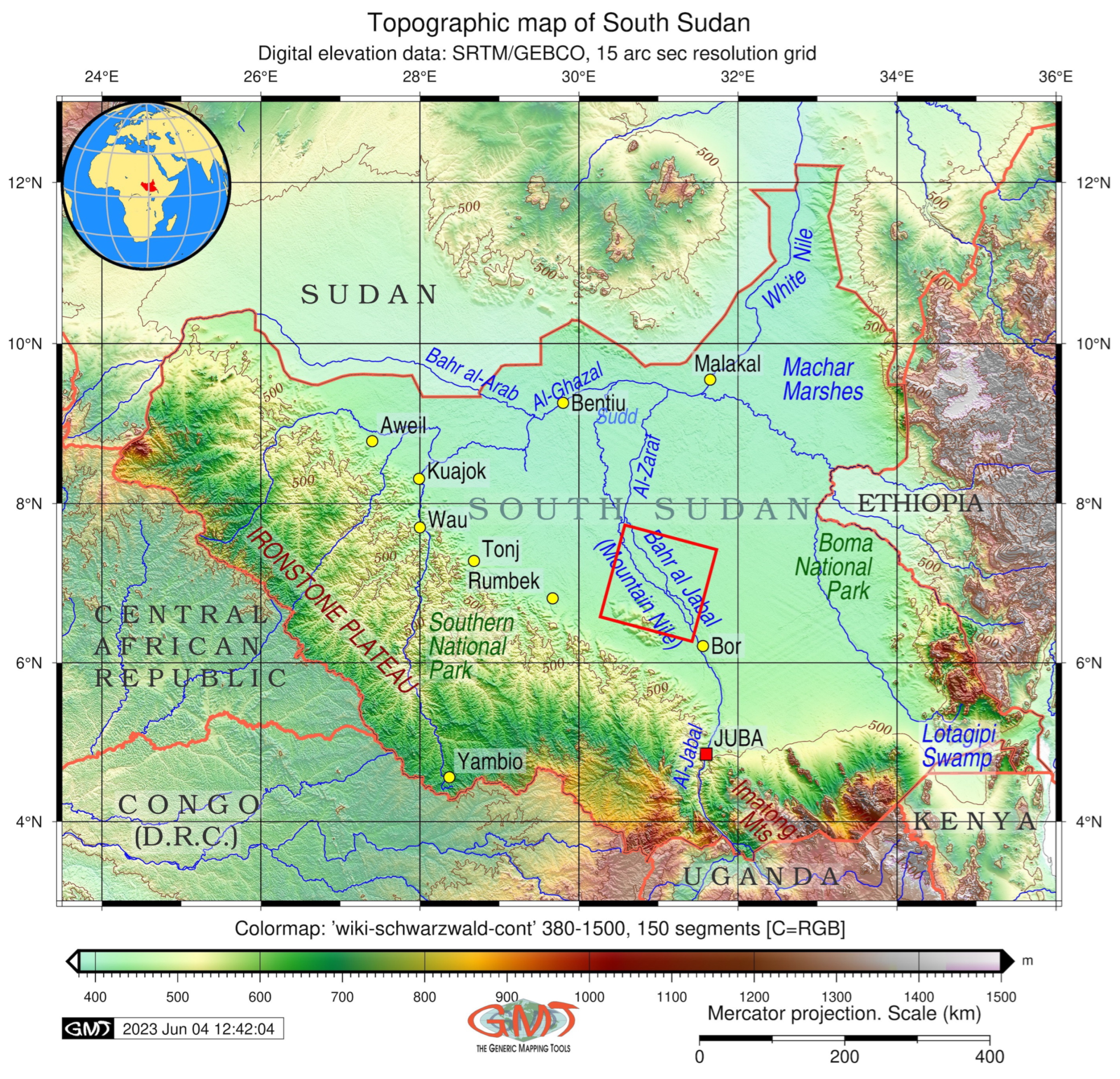
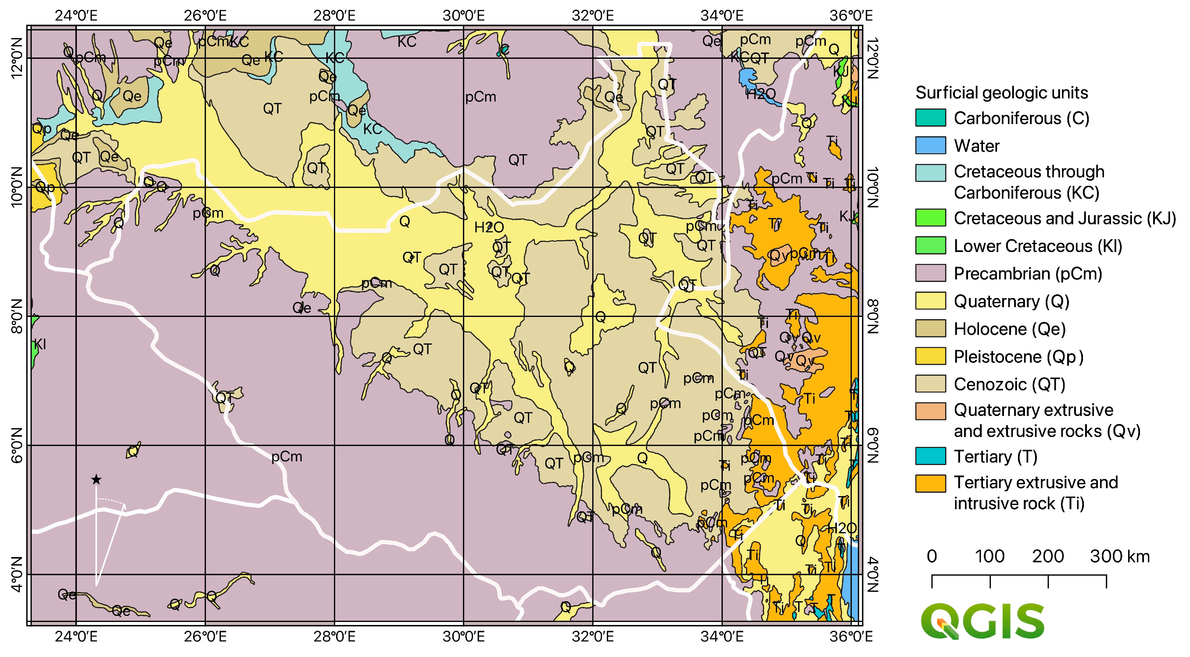
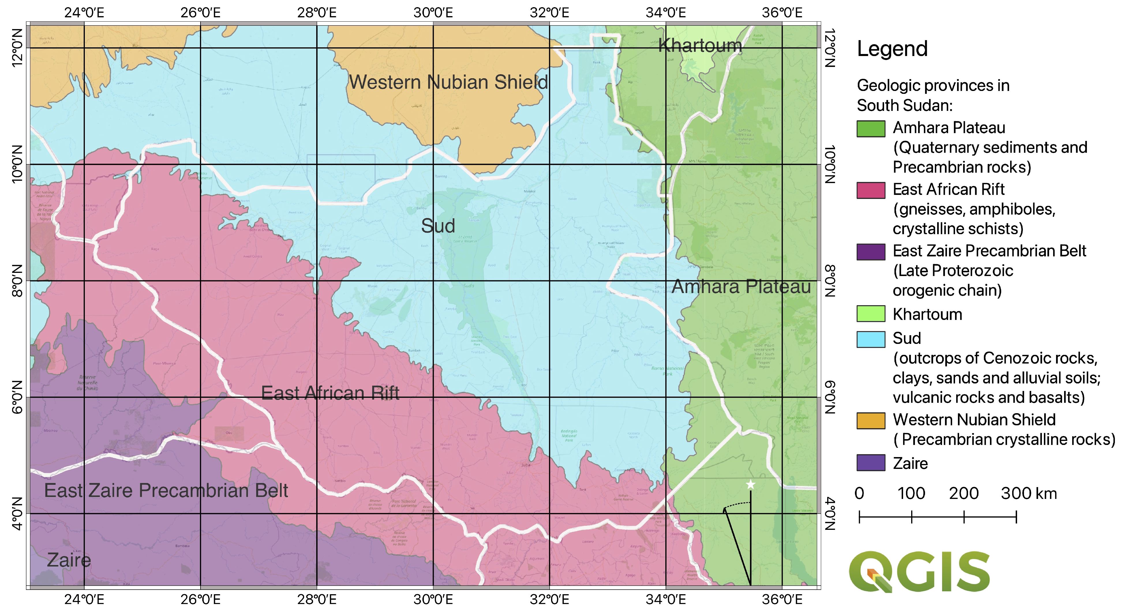
2. Characterisation of Study Area

The Sudd is a large area of wetlands located in South Sudan (Figure 1). The total area of swamp varyies between 30,000 to 40,000 km${}^2$ according to the wet or dry seasons [81]. The origin of these wetlands is strongly related to the geologic evolution of the Nile River basin, which affected the development of nearby landscapes [82]. Thus, the Sudd wetlands were formed in the course of the geologic development of the Upper Nile. Specifically, the study area is situated around Lake No, near the Bahr al-Jabal section of the White Nile (Mountain Nile), a branch of the Greater Nile [83]. Major geologic units include the Quaternary outcrops with clayey sediments of the Cenozoic (QT) Nile floodplain, shown in Figure 2.

The Nile River basin forms a part of the Great Rift Valley, which originated from a system of rift and faults with correspondent geomorphic forms, such as hilly areas, valleys, and plains [84,85]. Possible movements along these faults are reflected in the recent relief and the structure of the Quaternary sediment complex around the Sudd. The topographic analysis shows that the Sudd region has a contrasting relief, with river meanders having northward-oriented general gradient [86]. Moreover, the topography of south Sudan is strongly connected to the hydrology of the Sudd swamps, which is reflected in morphological features on seasonally flooded grasslands and slopes. The effects from topography and hydrology of the Nile, together with climate factors (precipitation, atmospheric circulation, and temperature), determined the formation of the wetland ecosystems of the Sudd. Thus, the plain geomorphology of the Nile floodplain provided perfect conditions for a series of basins which serve as reservoirs and accumulate water in the Sudd marshes during wet periods [87].

The Sudd wetlands are formed as a downstream of Lake Victoria and Lake Albert in the Nile Basin in the Sudd geologic province [88] (Figure 3). Recently detected diatoms proved the existence of the large Lake Sudd, which covered central and southern Sudan during the Holocene, when active tectonic structures significantly reduced their activity, acquiring the segmented character of the Sudd wetlands [89]. Other studies also reported the existing series of the interconnected basins along the Nile distributed over the territory of the modern Sudd province (Figure 3) during the Tertiary period [90]. Such palaeographic conditions contributed to further development of the current lacustrine environment in the Sudd. The dominated soil type in the Sudd wetlands is heavy clays and fine-grained sedimentary rocks [91]. Clayey soil creates favourable conditions for the formation of wetlands due to high impermeability and low porosity, which contribute to the accumulation of water [92]. As a consequence, a highly specific hydrogeological structure of the impermeable clays results in a very limited groundwater influence on the hydrology of the Sudd, where a top layer of vertisol is about 50 cm, and sands are distributed at depths of 30 m and below [93].

Climate factors affect the Sudd swamps through water balance [94] and evaporation [95]. The average temperature is 18.5 ${}^{\circ }$C, while the precipitation is 320 mm. High evaporation over the Sudd marshes results in strong effects on the regional water cycle of the Nile hydrology, which is amplified to a large extent by the Sudd wetland area: it is the largest wetland area existing in the world and the largest freshwater swamp region in the Nile Basin [96]. The environmental measures were undertaken to decrease evaporation from the Sudd by constructing Jonglei channels [97].

Climate effects on the Sudd wetlands are related to changes in precipitation and temperature: the increase in rainfall during the El Niño phases leads to warming and a rise in temperatures [98]. The dry season includes summer months, while the rainy season includes autumn–winter months. The transitional period is spring time. Climate factors threaten the hydrology and environmental sustainability of the Sudd wetlands [99]. Other climatic issues are related to the rise of Lake Victoria in 1960s, which triggered water losses in the Sudd [100]. The integrated effects from all these factors result in the highly unstable dynamics of the Sudd’s hydrology. Thus, the intensity of annual flooding differs significantly by years and affects the extent of the wetlands [101]. During the wet season, the Sudd increases in extent by almost twice due to the excess of water, which results in an extended area of floodplains affected by recurring inundation.

The Sudd wetlands play a strategic role in livelihoods, environmental sustainability, biodiversity balance, and the maintenance of water resources in South Sudan [102]. The value of the water resources in the Sudd relies on its economic and environmental services, high biodiversity impact, and fishery and food resources [103], which are necessary for social development and the existence of the local population [104]. At the same time, the ecosystems of the Sudd form a part of the global tropical wetland system, which is an important source of biodiversity and carbon storage in soils and vegetation [105], contributing to biogeochemical cycles and climate regulation [106]. The Sudd wetlands are known for hierarchical and complex food webs with diverse types of aquatic plants, animals, and microbial communities. The dominating vegetation types in the Sudd include papyrus, herbaceous plants, water hyacinth, marsh sedges, and grasslands [107]. Their distribution differs by habitat in the open-water areas with floating and submerged plants, as well as seasonally flooded grasslands occupied by the adapted plants.

Climate–hydrological fluctuations have cumulative environmental effects on the sustainability of the Sudd ecosystems. Thus, during the flood period, large areas of grasslands in the permanent Sudd swamps are inundated, which triggers fish migration into other sections of the floodplain [108]. Human-related factors affecting the Sudd ecosystems include overexploitation of the natural resources, increased pollution [109], landscape fragmentation [110], and habitat changes [111], which are reflected in the recent dynamics of land cover types in the Sudd region. At the same time, small grassland patches are hotspots of biodiversity in the fragmented landscapes and should be conserved for environmental sustainability [112].

3. Materials and Methods

In the following section, we present the scripting algorithm of GRASS GIS to process a series of satellite images through the powerful functionality of its tuned modules that are adjusted to diverse tasks of image processing and modelling. Our procedure works by running the script via the terminal command console shell, which makes it flexible and easier to handle and interpret the spaceborne data. Our pipeline then creates the set of commands used for image processing via the modules that include the multiline code snippets integrated in a script for image processing (Figure 4).

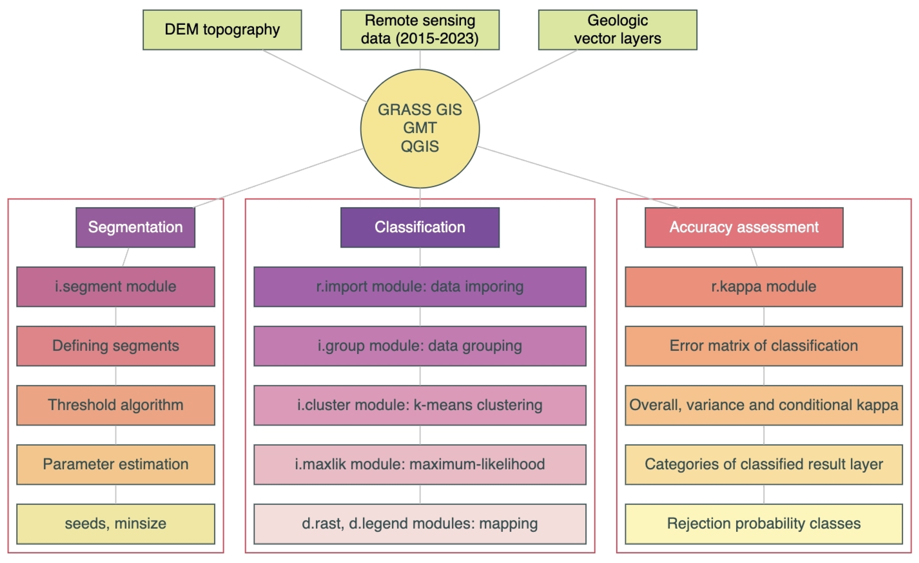
3.1. Software and Tools

A general scheme summarising the approach in this study is visualised in Figure 4. The data include topographic DEM, geologic layers, and remote sensing data processed with GRASS GIS, GMT, and QGIS. While the GRASS GIS tool was used for image processing, other software was used as an auxiliary tool for creating the methodology flowchart and topographical and geological mapping.

3.2. Data Collection and Import

The full dataset included in the framework is available at the United States Geological Survey (USGS) (Figure 5).

The Landsat images from 8 and 9 OLI/TIRS sensors were downloaded from the EarthExplorer repository: URL https://earthexplorer.usgs.gov/ (accessed on 30 July 2023). The EarthExplorer aims at Earth observation data, collected for the multiscale monitoring of Earth-related processes using remote sensing data. It is supported by the USGS, which coordinates and promotes storage of the datasets in digital format for queries. It enables downloading the satellite images and provides cartographic information for data. Besides Landsat, it also supports other remote sensing products, such as radar data, aerial imagery, Digital Elevation Models (DEM), Advanced Very High Resolution Radiometer (AVHRR), etc. The reason for the nine satellite images consists in demonstrating the dynamics of the land cover types within a comparable period. Another reason consists in the available images with low cloudiness, which are below 10% for the scenes takes in the appropriate seasons.

The images cover 9 years, from 2015 to 2023, Figure 5. These years were chosen for the two following factors: the availability of the cloud-free images or those with minimised cloudiness (below 10%) and the gap between the years enabling the comparison and analysis of environmental dynamics. The choice of image data is explained by the two criteria: (1) the cloudiness of the image is below 10% for all the scenes; (2) the images are captured in the dry period to objectively assess the postflood scenario. The wet period of the Sudd region is accompanied by heavy rainfalls that last throughout the summer period. The exact period differs significantly by year and, according to various information sources, may last between April and September [113] or from March to October, according to the Climate Change Knowledge Portal. The data import was performed using the ‘r.import’ command in the GRASS GIS module. The scripts are shown in Appendix A of this study with the code for data import.

The greatest concentration of rainfalls in the Sudd is recorded between June and September [114]. Therefore, all the images were taken during the dry period to avoid the months from June to September. Since flooding and seasonal dynamics vary yearly, each scene was inspected to evaluated the quality and distinguished contours of the diverse land cover types. Each Landsat OLI/TIRS image included eleven spectral bands in visual, panchromatic, and near-infrared channels. Besides the satellite Landsat images, this study also included auxiliary data, such as topographic data (GEBCO/SRTM grid), geologic USGS data, and descriptive information from textual sources regarding the social and economic activities in the Sudd region, as well as statistical and descriptive environmental reports on South Sudan available online), which were used for environmental analysis.

3.3. Data Preprocessing

The overview topographic map of the study area shown in Figure 1 was mapped using the Generic Mapping Tools (GMT) software version 6.1.1. [115]. The applied GMT scripting technique was derived from the existing works [116,117]. The geological maps were plotted using QGIS. The remaining workflow was performed using the GRASS GIS using diverse modules, following existing similar works using GRASS GIS in environmental applications [118,119,120,121]. A folder with the uploaded Landsat imagery was stored in the ‘Location/Mapset’ working directory of the GRASS GIS with relevant subdirectories. Here, all the map layers were located and hierarchy-supported for imported satellite images following the standard GRASS GIS workflow [122]. The codes were written using the Xcode and run from the GRASS GIS console. The files were imported in TIFF format using Listing A1 and stored in the WGS84 coordinate system.

The atmospheric correction method included the algorithms of the embedded GRASS GIS module ‘i.landsat.toar’. This module enables to convert the DN pixel values to reflectance values using DOS1 from Digital Number (DN) to reflectance. Before creating an RGB composite, it is important to perform the atmospheric correction and thus convert the digital number data (DN) to reflectance or radiance. Otherwise, the colours of a natural RGB composite do not look convincing but rather hazy. This conversion is performed using the metadata file which is included in the dataset with i.landsat.toar, which calculates the top-of-atmosphere radiance or reflectance and temperature for the Landsat MSS/TM/ETM+/OLI.

The general outline of the data processing includes data capture of the Landsat 8-9 OLI/TIRS images, data preprocessing, data conversion, segmentation, classification, validation, computing the land cover classes by covered area, and mapping. The workflow aimed at detecting variations in the wetland areas and identifying the extent of the flooded area in the Sudd marshes over the nine-year period. For a comparison of gradual changes, a one-year interval was selected between each pair of images. To ensure that technical requirements of code quality are met, several tests were carried out for Landsat images on various years using different parameters of segmentation threshold. This aimed at analysing the behaviour of the algorithm for various levels of image fragmentation using different threshold levels. The obtained image samples were stored in a separate folder of the GRASS GIS with a path to the working folder of the repository.

3.4. Metadata and Extent

A dataset of the nine Landsat 8-9 OLI/TIRS images containing TIFF raster files was analysed for metadata, with the parameters summarised in

Table 1. Metadata for Landsat 8-9 OLI/TIRS images.

Proj.	Zone	Dat.	Ellips.	N	S	W	E	Nsres	Ewres	Rows	Cols	Cells
UTM	36	WGS84	WGS84	915,615	682,785	190,785	419,115	30	30	7761	7611	59,068,971

Abbreviations in Table 1: Proj—projection; Dat.—datum; Ellips—ellipsoid; N—north; S—south; W—west; E—east; nsres—resolution in north–south direction; ewres—resolution in east–west direction; cols—columns.

. The Landsat images were taken on the following periods: 8 January 2015, 12 February 2016, 31 December 2017, 1 February 2018, 8 March 2019, 26 March 2020, 29 March 2021, 19 January 2022, 14 May 2023.

Visual bands of the original Landsat images (channels 1 to 7) were uploaded in TIFF format, processed and converted into several segments. The region extent and groups of the bands were defined on the Landsat images using the parameters in the scene by the snippet of code presented in Listing A2. The region borders for the Landsat scenes covering the Sudd area are as follows: north: n = 915,615; south: s = 683,085; west: w = 185,985; east: e = 414,315.

3.5. Defining Segments

The approach of the GRASS GIS to image segmentation is based on the use of the module ‘i.segment’. The algorithm groups similar pixels on the satellite image into unique segments. The thresholding algorithm assigns pixels on the image based on the similarity between two neighbour segments and detects the segments. This enables the detection of the flooded area and automatically recognises changes in the landscapes. The segmentation was performed with a 90% threshold and minsize = 5; the process was converged in 41 iterations. The process was completed in 50 min for the Landsat satellite image for 2023. The region IDs were assigned to all the regions, including the remaining single-cell regions. Overall, 8464 segments were created for one Landsat image (2023).

Afterwards, the minimal size was changed to 100 to check the effects from the modified parameters on the results of the segmentation process. For modified parameters, the seeds were used to optimise the procedure and to provide the basis information for image classification. These included random segments which were selected automatically using previous segmentation rounds and used to start the segmentation process anew, using the code shown in Listing A3.

3.6. Threshold Algorithm

The threshold algorithm searches for the bounds of each segment on the image and plots the image generated using threshold parameters according to the similarity level below the input threshold for a coarse analysis. The rise of threshold level increases the fragmentation of the segments accordingly; see Figure 6. In turn, if the similarity distance is smaller, the pixels are assigned to other neighbour segment. Afterwards, the algorithm sets a start–end position, and the process is repeated iteratively until no more merges are possible for the segments of landscape patches during a complete pass of image segmentation. The segmented image is then visualised using the code in Listing A4 and saved as standard TIFF output format in full-resolution mode using GRASS GIS. The information on the Landsat scene is retrieved from the file, and the segments are visible in the visualised image.

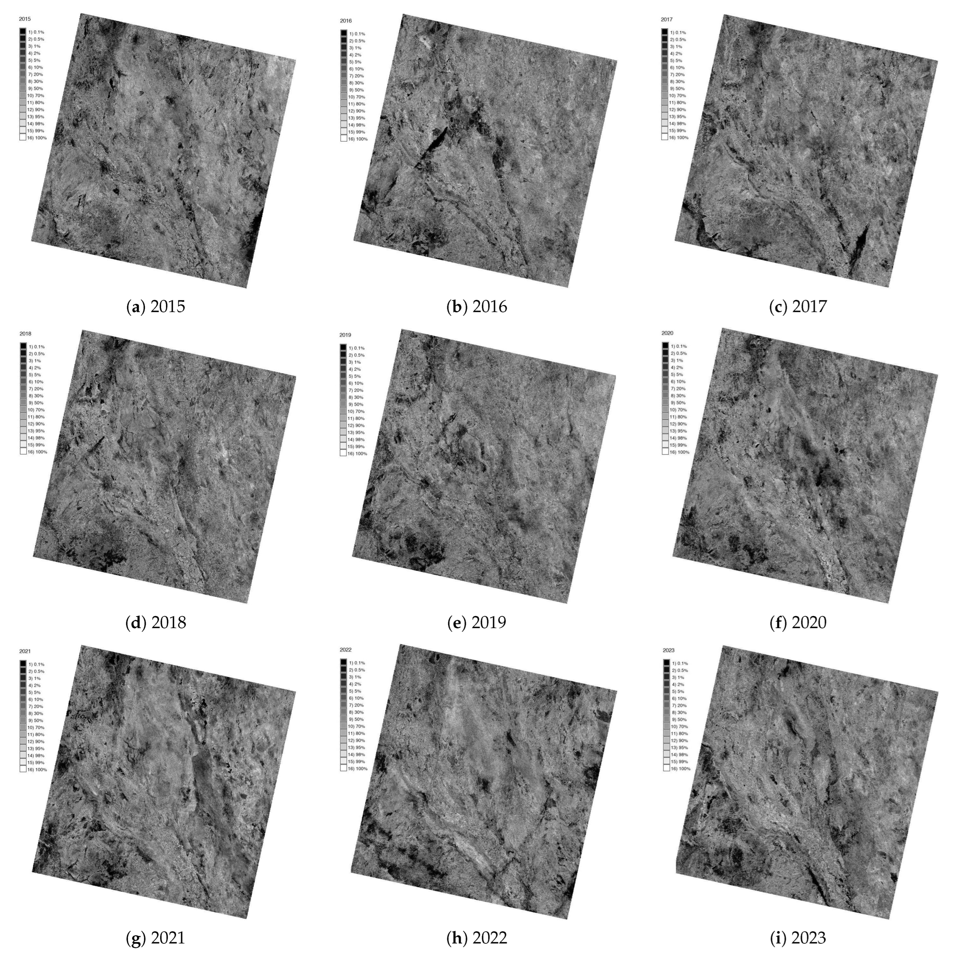
3.7. Image Segmentation

The images resulted from the segmentation at the two levels of threshold are shown in Figure 6. The code for processing the image with script is based on defining the objects through image segmentation that contains patches of regions with similar parameters of the pixels located inside. Here, the similarity between the current segment and each of its neighbours is computed using a search algorithm, which includes the given distance formula for a target segment. The processing of these segments is possible at both high and low threshold modes and defined similarity parameters. It displays merged segments if they meet technical criteria and analyses the coverage of the valid segments using the algorithm function on an image. Then, it computes the position for each pair of the segments, which shows the best mutual similarity in a target region of the image using iteration for each next region.

Accordingly, the search for the closest segment is based on a similarity between the segments and objects. In such a way, the algorithm is propagated along the image, searching for every consecutive object iteratively to determine which objects are merged. The values of the smaller distance between the objects were evaluated to indicate a closer match within each iteration on the image. Thus, a similarity score of zero is assigned for identical pixels which are assigned to an identical segment. In case of the lower threshold of segments on the images, the similarity between the two segments is lower than a given threshold value. In such a case, the combination of these region is performed using the minimal size parameter. According to this principle, all the segments with a lesser number of pixels are merged with their similar neighbour. Such an approach enables the optimisation of segments through the distribution of the array of pixels into the segments.

3.8. Parameter Estimation

The estimation of segmentation parameters was based on the tested variants of the threshold value of the segments in a relative number, which is always between 0.0 and 1.0. A changed degree of segment fragmentation is visible in trial cases (Figure 5). The tested segment size has a thickness varying from a threshold = 0.90 to a threshold = 0.05, and a seed minimal size is defined at 100 pixels. The repetitive iterations described above divided the image into several segments, indicating land cover classes. The resolution of 30 pixels for the Landsat image is used as the optimal parameter for a given landscape patch, allowing one to indicate small segments on an image. A lower threshold allows only large groups of vegetation to be merged using valued pixels with similar spectral reflectance values. In contrast, a higher threshold (close to one) allows neighbouring land cover classes to be merged. Thus, the threshold level of image segmentation is scaled to the actual data range.

To reduce the noise effect and to optimise data processing, a minimal size greater than one was added as an additional step of image processing. During this step, the threshold of segmentation is ignored to avoid too fragmented images. Thus, for segments smaller then the defined size, this parameter merges tiny patches with their most appropriate neighbours. In such a way, the original Landsat scene is partitioned by the complete image according to the values of the pixels’ colour and intensity. The process of thresholding was based on the analysis and separation of the pixels compared against the value of the minimum segment size. It aims to discriminate the meaningful part of the image containing landscape patches from the noise pixels.

3.9. Clustering

The performance of the segmentation was a slow process and required further postprocessing for identification of the land cover classes within the Sudd area. To address this, a three-step process was implemented: First, the segmentation was executed as discussed in the previous subsection. This produces segments that include identity grid pixels, in which we expect to landscape patches. The grid cells were then generalised, and the classification process was performed using the ‘i.maxlik’ module, which uses the maximum-likelihood discriminant analysis classifier. Third, the accuracy assessment is performed using the GRASS GIS module ‘r.kappa’, which computes error matrices and kappa parameters for accuracy assessment of classification for each Landsat scene. The code for the maximum-likelihood classification is presented in Listing A5.

The clustering algorithm approach by the ‘i.cluster’ module is a powerful tool for image partition prior to classification. It operates on an image using defined parameters, such as initial number of clusters, minimum distance between them, coherence between loops, and minimum area for each cluster. The robustness of clustering is tuned by the correspondence between the iterations and the defined maximum number of loops. The initial cluster means for each band are defined by values of the first cluster as a band mean corrected for standard deviation, and all other clusters are distributed equally between the first and last clusters, as implemented in GRASS GIS.

The flexibility of clustering is that all clusters less than the defined minimum are merged smoothly, which outperforms similar algorithms of image partition. Hence, the clusters are regrouped accordingly in the iterative way. Here, each pixel is assigned according to the closest distance to a given cluster using the algorithm of Euclidean distance, and the results are saved in a signature file, which is then used for classification by the ‘i.maxlik’ module of GRASS GIS. The clustering report is generated automatically for an image, with an example presented in Appendix C. Thus, clustering presents the advanced object-based detection method. which creates signatures for the next step of image classification, which computes the distance between pixels using the similarity method.

3.10. Classification

Afterwards, the maximum-likelihood discriminant analysis classifies the generated clusters, segments and covariance matrices, computed previously. These are used to define categories of each evaluated cell. The 30-resolution remote sensing imagery corresponds to the following land cover types in the Sudd region [123]: (1) Cropland; (2) Herbaceous coverage; (3) Forest; (4) Mosaic tree canopies; (5) Shrubland; (6) Grassland; (7) Flooded and inundated areas; (8) Bare areas; (9) Built-up areas; (10) and Water areas. These land cover types were used for landscape analysis. Hence, the pixels are assigned to the categories of the land cover classes according to the calculated highest probability of belonging to the given class on the image based on their spectral reflectance. The assignment of pixels into classes of land cover types is based on the signature file (“signaturefile”), which contains the cluster and covariance matrices calculated by the module ‘i.cluster’ and is shown in Listing A5. In such a way, the maximum-likelihood classifier partitions the total number of pixels on the whole Landsat scene using the segmentation and clustering results as preprocessing steps for image classification that sequentially examine all current segments in the raster map.

The pixels were grouped into segments representing land cover types as separate segment objects, and the map is generated for each Landsat image from 2015 to 2023 using the maximum-likelihood discriminant analysis approach of classification. The description is created for the segments of each land cover type of the Sudd in the relevant images. The segments of land cover classes which have a sharp transient from neighbouring class are considered as another category. Afterwards, valid segments in connected landscapes are regrouped using the trial tests for various threshold parameters. The segments from the Sudd landscapes are combined into maps and compared for various years from 2015 to 2023. The distinct classes are detected using the GRASS GIS algorithms iteratively for each segment using image analysis.

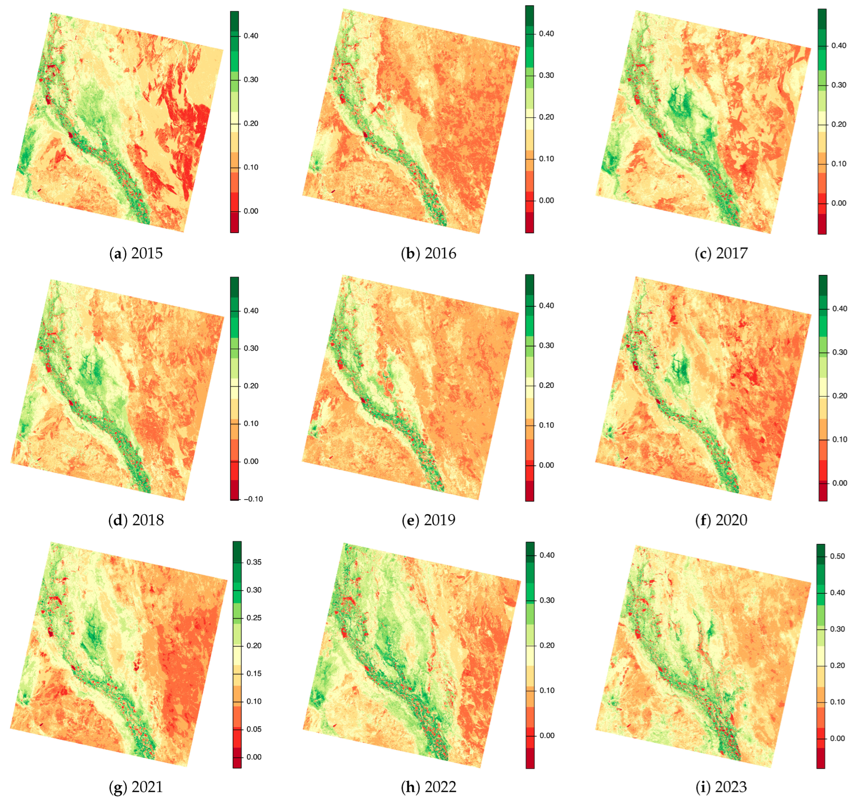
3.11. Calculating the NDVI

To evaluate the distribution of healthy vegetation over the study area in the postflood scenario, the NDVI was computed using the script in Listing A6. For atmospheric corrections, the values of the Digital Number (DN) of the pixel were converted to reflectance values using DOS1 to avoid a hazy background. This conversion is performed using the metadata file which is included in the dataset with ‘i.landsat.toar’ and information about the sun elevation for each scene. Using the ‘i.landsat.toar’ module, the top-of-atmosphere radiance and temperature were corrected for the Landsat OLI sensor. Afterwards, the NDVI was computed using the existing combination of the Red and NIR bands of the image, and the images were visualised using the script presented in Listing A6.

3.12. Accuracy Assessment

The accuracy assessment was performed in two ways. First, the error matrix and kappa parameters were computed by the ‘r.kappa’ module of GRASX GIS. Second, the rejection probability classes were calculated to estimate the pixel classified according to confidence levels based on the classification of the satellite images. This was implemented using the ‘i.maxlik’ module and resulted in plotted maps showing the rejected threshold results, as shown above in Listing A5. The confusion matrix was estimated by kappa with computed possible misclassification cases and derived kappa index of agreement. This was performed using the code in Listing A7.

Image processing by GRASS GIS also included the removal of the noise signals from the images through the adjusted segmentation threshold and image partitioning into segments for monitoring inundated areas and classification. The results of the kappa calculation are presented as confusion matrices in a tabular format (kappa.csv). These tables were computed for each classified Landsat image and present the calculation results, reporting data for every category of land cover classes, as summarised in the Appendix B.

4. Results

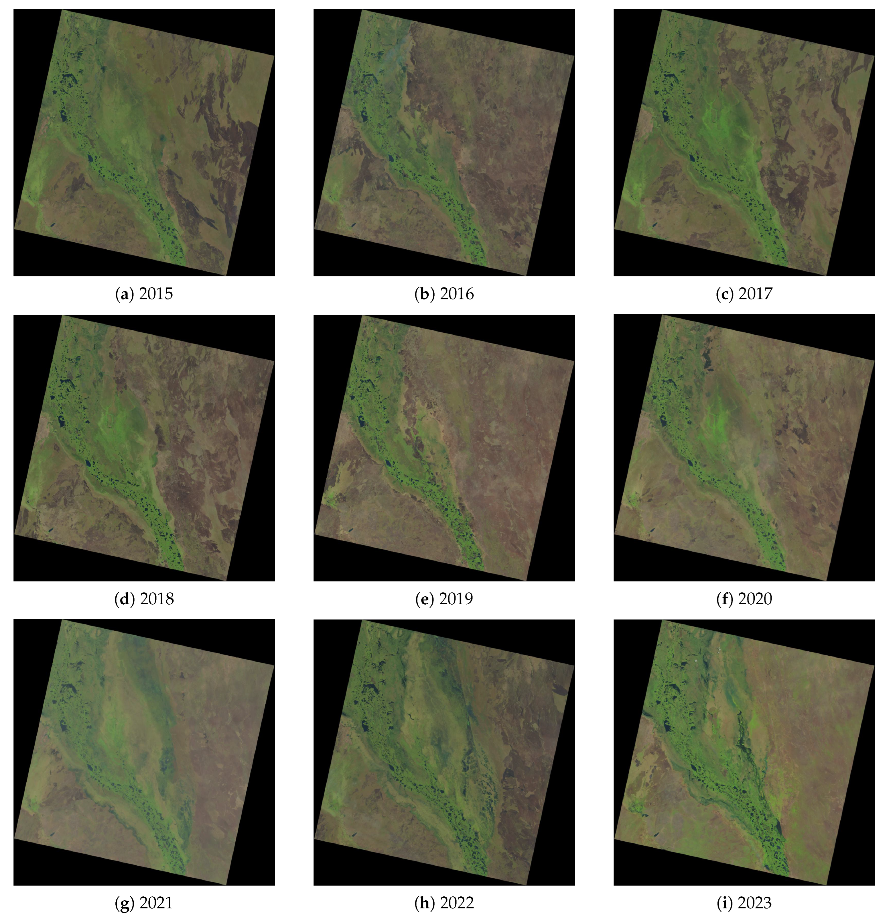
4.1. Remote Sensing Data Analysis

The algorithms of the GRASS GIS described above and summarised in scripts were applied to process the Landsat satellite images, with the results of the segmentation shown in Figure 6. Scenes were segmented for each year with the visualised maps. Remote sensing data organisation and management were performed using the GRASS GIS software. It presents a multifunctional GIS as well as workspace and editing system for remote sensing and cartographic data storage and processing [122]. Its effective functionality enables one to perform various steps of image processing and spatial data processing: storage and organising, navigating and visual inspection, projecting, formatting and converting, image analysis, handling metadata adding annotations on maps, visualising and analysing diverse features related to Earth observation data, and mapping. Other advantages include open-source availability and double-mode functionality: using either scripts or a Graphical User Interface (GUI). Moreover, GRASS GIS enables one to operate large datasets in vector and raster formats. Here, each folder of Landsat images contained 800–900 MB, which resulted in the processing of 9 Gb for nine satellite images, effectively processed by the GRASS GIS.

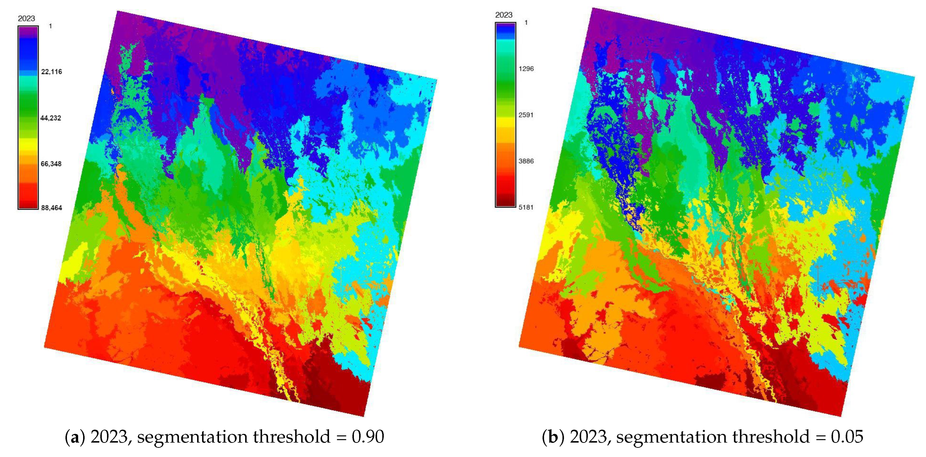
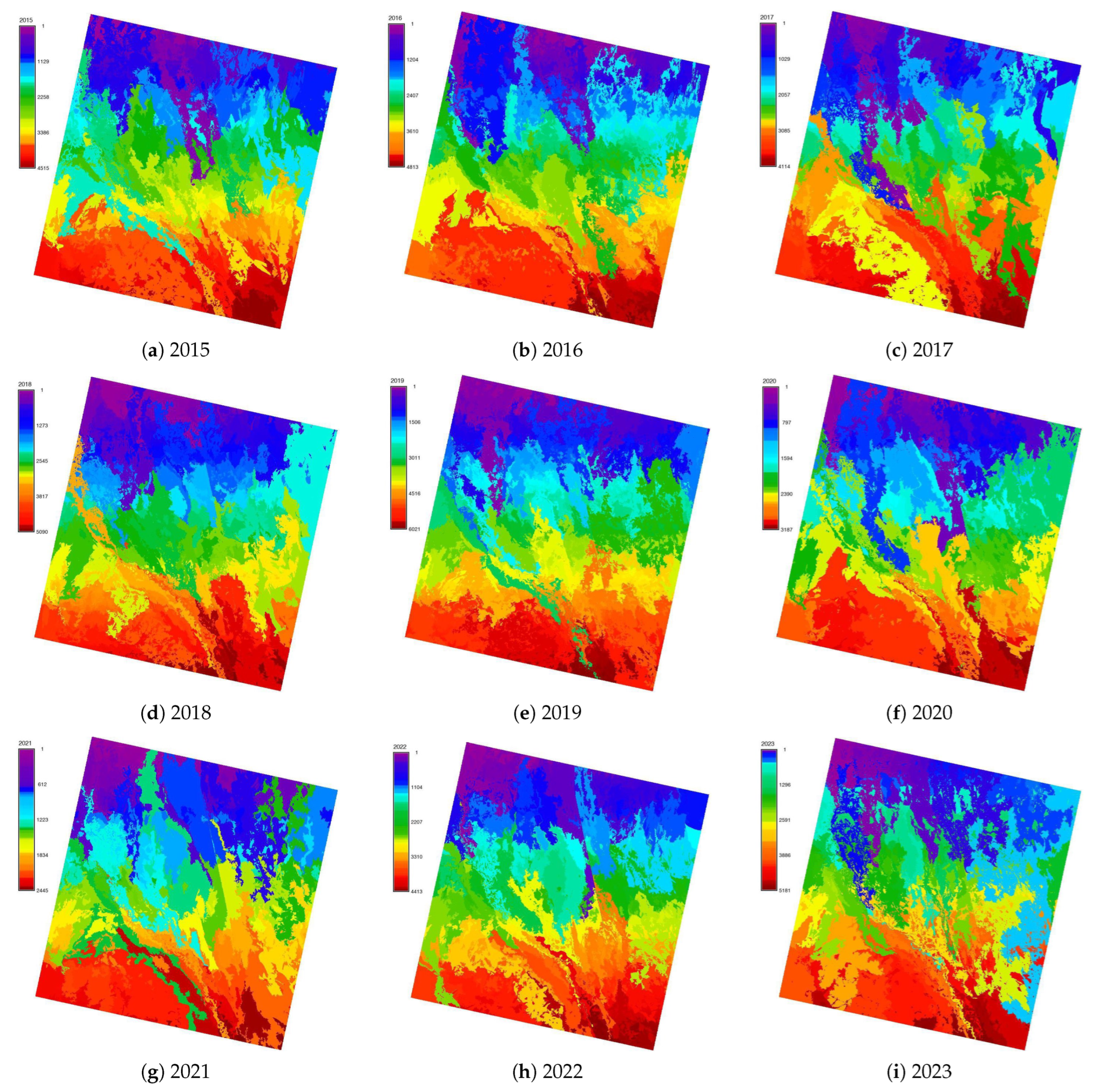
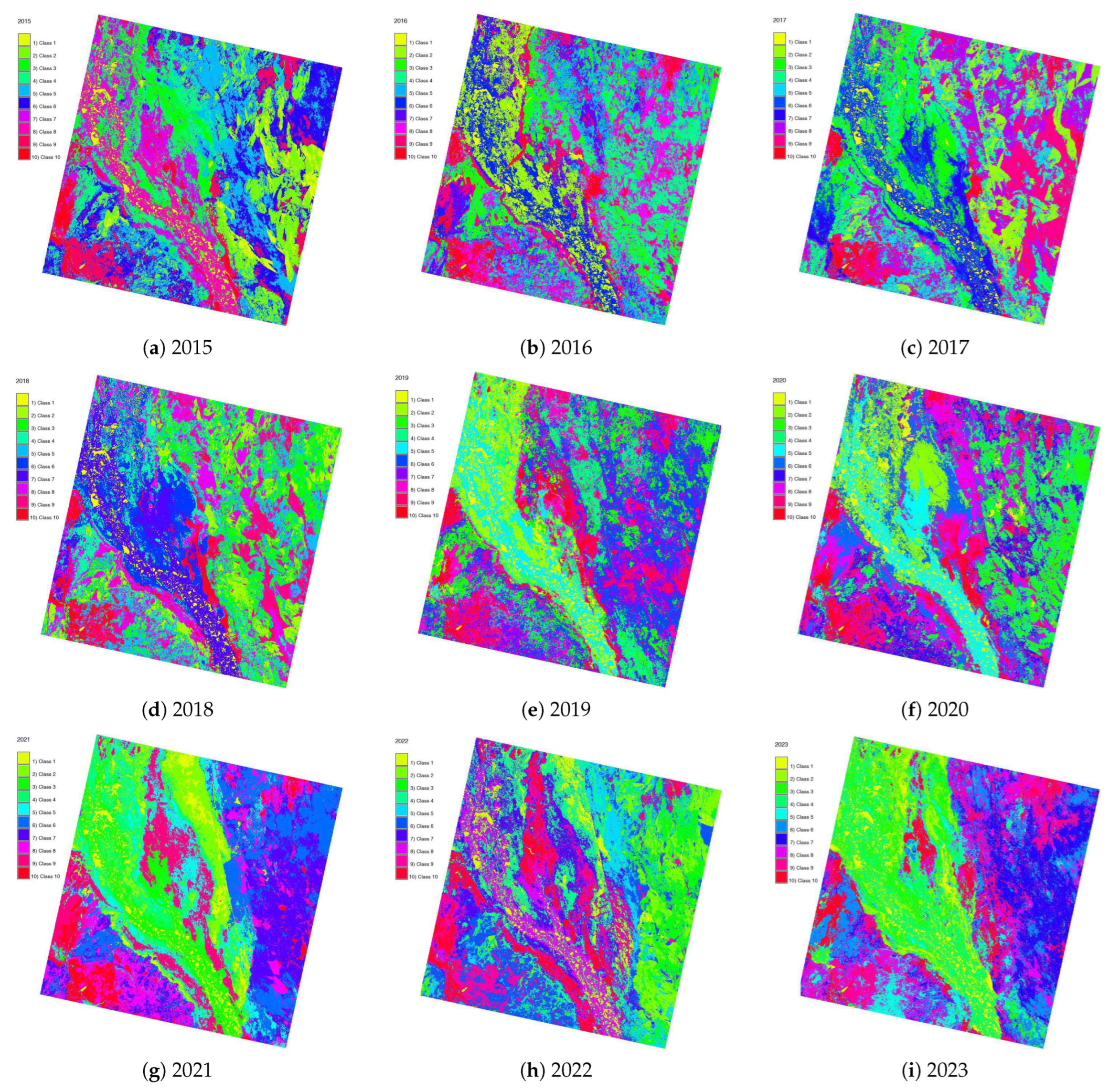
4.2. Detection of Segmented Areas

The results of Landsat 8-9 OLI/TIRS image segmentation are presented in Figure 7.

The computed areas by land cover classes and their changes by years are summarised in

Table 2. Computed areas of land cover classes derived from the classified Landsat 8-9 OLI/TIRS images for the region of the Sudd, South Sudan in the period from 2015 to 2023.

Year	Class 1	Class 2	Class 3	Class 4	Class 5	Class 6	Class 7	Class 8	Class 9	Class 10
2015	1,501,537.8	243,574.1	317,231.5	17,077.0	241,763.7	734,523.3	447,070.3	528,704.9	466,546.4	281,024.0
2016	606,130.3	594,056.0	251,200.3	478,775.3	108,958.6	202,940.2	558,836.7	132,573.3	471,370.5	386,764.2
2017	344,062	395,409.0	458,500.0	458,986.4	526,807.8	540,912.0	761,353.5	468,330.1	664,728.9	873,149.5
2018	427,690.5	1,054,373.0	1,083,009.3	881,093.1	881,190.4	705,596.0	526,685.1	315,125.8	1,128,926.5	495,258.0
2019	376,759.4	332,136.8	251,513.7	982,144.2	124,956.3	757,819.1	1,090,100.0	625,188.6	109,114.2	689,025.5
2020	272,113.4	180,816.8	419,207.8	402,059.3	493,457.7	1,156,585.4	937,007.5	584,898.4	1,567,576.9	752,311.4
2021	416,413.7	234,023.4	189,669.0	414,165.1	490,691.7	578,060.7	118,864.8	467,398.9	283,889.0	355,065.7
2022	307,658.6	1,168,006.6	147,964.0	423,542.0	617,279.5	442,903.9	383,683.5	788,245.4	770,970.0	267,592.8
2023	0.0	29,203.0	1,599,665.7	434,129.5	1,012,475.1	1,032,878.3	934,255.0	1,214,757.6	167,164.5	687,965.9

. The classes signify the following land cover types: (1) Cropland; (2) Herbaceous coverage; 473 areas (3) Forest; (4) Mosaic tree canopies; (5) Shrubland; (6) Grassland; (7) Flooded and inundated; 474 areas; (8) Bare areas; (9) Built-up areas; (10) Water areas. These land cover types were used 475 times for landscape analysis.

A multiscale time series analysis demonstrated changes in flooded areas of the Sudd region, revealed in the maps by gradual changes in the landscapes, which are visible on the segmented Landsat images taken yearly from 2015 to 2023. For the Landsat 8-9 OLI/TIRS scenes, the results of the image segmentation performed using the identical parameters defined for all the images are summarised in

Table 3. Results of the segmentation procedure for Landsat 8-9 images with No of created segments.

Year	Scene ID	Iterations	Segments
8 January 2015	$LC08\_L1TP\_173055\_20150108\_20200910\_02\_T1$	37	4515
12 February 2016	$LC08\_L1TP\_173055\_20160212\_20200907\_02\_T1$	37	4813
31 December 2017	$LC08\_L1TP\_173055\_20171231\_20200902\_02\_T1$	38	4114
1 February 2018	$LC08\_L1TP\_173055\_20180201\_20200902\_02\_T1$	36	5090
8 March 2019	$LC08\_L1TP\_173055\_20190308\_20200829\_02\_T1$	34	6021
26 March 2020	$LC08\_L1TP\_173055\_20200326\_20200822\_02\_T1$	39	3187
29 March 2021	$LC08\_L1TP\_173055\_20210329\_20210408\_02\_T1$	35	2445
19 January 2022	$LC09\_L1TP\_173055\_20220119\_20230501\_02\_T1$	35	4413
14 May 2023	$LC09\_L1TP\_173055\_20230514\_20230514\_02\_T1$	41	5181

Notation for Table 3: The Landsat images were selected with cloudiness below 10% to achieve maximal distinguishability of the contours of the images.

. Here, the number of iterations (passes) depends on the level of fragmentation of the image and varies by years. Segmentation and processing of the Landsat 8-9 OLI/TIRS datasets by GRASS GIS served for detecting flooded areas and monitoring the inundated areas in the Sudd marshes. The detected large seasonal changes in wetlands result from variation in the flow of Nile tributaries and Victoria Lake, as well as climate–hydrological pulsing. The approach is based on the analysis of landscape patches, grouping segments on the images, and hierarchical clustering (subgroups of landscapes using various threshold levels) for classification following image segmentation (Figure 7).

Detecting and recognising the segments on the Landsat images implies identifying the fields of regions which correspond to the 10 major land cover types in the Sudd wetlands of South Sudan. These regions are grouped into semantic categories (landscape patches and land cover types). The hierarchical level of the geometric objects with regard to their scale (small-, middle-, and large-size) was applied, and the threshold was optimised. The detection of segments on the images was based on the mean shift image segmentation, including filtering and clustering (Figure 7). Since both algorithms are embedded in the ‘i.segment’ module, the images were segmented without the priori landscape-dependent information, which ensured independent interpretation.

The grouping decision is made using the features of pixels that match target classes (‘segment’/‘not segment’), colour, distance to the threshold in pixels, and the spectral reflectance of the pixel. The shape of the segment is defined through the boundary constraints, which limits the adjacency of pixels and segments on a satellite image. In such a way, the image is represented as a vector geometric structure, recognised and identified by a computer vision approach. The assessment is based on the connectivity of pixels constituting the segment, except for the threshold fitness and the difference between several segments, which break the image scene into a mosaic of patches.

Defining the segments on an image series enabled us to detect inundated areas after flood disasters and compare changes in complex channel and lagoon systems within the area of the Sudd marshes (Figure 8). The areas covered by water are distinct from the neighbour regions and only include pixels with corresponding spectral reflectance for water, which shows a contrast between the red and near-infrared (NIR) areas. The segments show the location of the Bahr al Jabal flow and its floodplain with distributed small tributaries separated based on the values of pixels, which are different from the forest land cover types or those covered by agricultural vegetation. The consequences of the flood events are visible on the corresponding image scenes by an analysis of land cover changes. Thus, the changed pattern of the postflood landscapes as a consequence of severe floods in July 2014 triggered by seasonal rainfalls is visible in the image in Figure 8a. Social consequences of such disasters include worsened living conditions and the displacement of 68% of 1.3 M people [124].

Winter months after the annual flood peak are characterised by the saturated soils with the highest moisture level, which cannot retain additional water due to the reached saturation level. Therefore, even minimal rainfall triggers further catastrophic flooding and results in chained consequences. Thus, occasional rainfalls contribute to the high level of inundated lands (Figure 8b–d). Flash floods and heavy rains between June and November 2018 affected over 142,000 people, with damaged households and livelihoods [125]. The consequences of these disasters with flooded grassland ecosystems and inundated areas (bright green areas) are visible in the image taken in early 2019, shown in Figure 8e. Abnormally heavy seasonal flooding in South Sudan in July 2019 devastated large areas of the Sudd and surrounding areas of the White Nile tributaries, swamps, and lakes [126]. The postflood image in early 2020 shows inundated areas and landscapes (Figure 8f).

The increased in flooded areas (bright green areas; Figure 8g) resulted from the worst floods in Sudan in August 2020, which were reported by the United Nations Office for the Coordination of Humanitarian Affairs (UN OCHA) [127]. The social consequences of such events are around 600,000 people being affected by disasters along the White Nile since July 2020, and widespread flooding continued in until autumn 2020. The largest affected state is Ayod, with 150,000 affected and displaced people due to the flood’s effects. The affected land cover changes are reflected in the postflood image of March 2021, shown in Figure 8g.

The NDVI maps for a time series of the images show the distribution of vegetation in the postflooded scenario, shown in Figure 9. The floods in August 2021 represent the disaster in the Sudd due to the heavy showers in southwestern South Sudan, resulting in floods and river overflow. The flooding in 2021 was particularly dire in central regions of the country along the Upper Nile region, including the Jonglei state where the Sudd area extends [128].

The social consequences of floods for the local population are reported accordingly [129]. It is also noted by the World Health Organization (WHO) [130] that severe floods in July 2022 resulted in evacuations and damage to one million people, and 7380 people were displaced in South Sudan. The consequences for infrastructure include blocked routes by increased flood waters, which disabled humanitarian actions. The southern part of the country, including Bentiu and Jongleis state, were the most affected. The increased inundated areas as a postflood consequence in 2023 are visible as bright-green-coloured areas, shown in Figure 9i. To evaluate the rejection probability classes, maps of pixels classified according to confidence levels were made based on the classification of nine satellite images, shown in Figure 10.

Spectral information relevant to land cover classes is obtained from the landscape analysis of the Sudd area, while the information on flooding detected in each image is retrieved through segmentation. The land cover classes are identified during classification using the distinct colours of segments and constructing the morphological shapes of the represented objects (e.g., the flow of the Nile River) in each of the images. All the pixels encompassed inside each segment are identified iteratively by the machine and interpreted accordingly. The information from landscape patches is used to find the variations by years and propagate inundated areas using comparative analysis. Afterwards, the segments are identified as land cover classes for each segment of the image, and the metadata of the segments are updated for each scene accordingly.

5. Discussion

5.1. Advantages of the Tools

This paper presents an alternative algorithm of scripts-based remote sensing data analysis for environmental modelling. A multiple-methodology approach was applied to various steps of research. Image segmentation, classification, NDVI calculation, computing land cover classes, and validation of the results with accuracy assessment were performed using the GRASS GIS using a time series of the Landsat satellite images, while the QGIS was applied for geological mapping, and the topographic map was plotted using GMT. The presented series of maps supports the evaluation of the environmental setting in the Sudd region, South Sudan. Thus, based on the satellite computations of the flooded area in the Sudd, the obtained maps estimated the extent of 10 major land cover classes and flooded areas, with notable extent especially in the years 2016, 2018, and 2020. Additionally, the maximum flood extent occurs early, with an earlier peak in the flooded extent of inundated areas, which is related to the Sudd’s hydrodynamics. Thus, the expanded flooding in the wetlands of the Sudd might have caused backwater effects that affected the wetland’s extent and behaviour.

In this way, the current paper contributed to monitoring the Sudd wetlands through image analysis, including segmentation and classification, with the aim to determine landscape changes over the past nine years. The important deliverables of this work include image segmentation and classification to identify the diverse land cover classes for analysis of vegetation and flooded areas based on image analysis techniques. In contrast to the former reported results [131] where low-resolution SAR imagery was used and processed using ENVISAT software for the period of 2007–2011, this study presented a scripts-based approach using an open-access high-resolution dataset, which enables the repeatability and continuation of this study. Previous works also reported an increase in peak flood area, which ranges considerably from 2007 to 2009, and classified permanent flooding, seasonal flooding, and intermittent flooding areas. Likewise, this study reports an increase in the inundated areas of the Sudd for the years 2016, 2018, and 2020.

5.2. Key Deliverables

The wetland systems of the Sudd are one of the most important ecosystems of South Sudan and are included in the list of the Ramsar Convention on Wetlands of International Importance Especially as Waterfowl Habitat due to their hydrological importance in the Nile Basin, as well as the high number of endangered and vulnerable species therein. The Sudd plays a crucial role in regulating the balance of floodwater and accumulating sediments from the Mountain Nile. Moreover, since over half of the water is evaporated in the Sudd, it serves as an important mechanism of hydrological stability in the Nile River. Therefore, the disturbed flooding system will necessarily affect the Nile Basin and involve negative environmental consequences. The decrease in wetland area and the changed hydrological regime of marshes can directly and indirectly affect the Nile Basin and thus increase the negative effects of climate change. In this regard, conservation actions focused on the Sudd wetlands support the regulation of the following climate–environmental issues: increase in temperatures, unstable precipitation patterns, unbalanced crop planting, deforestation, carbon emissions related to regional agriculture sector, etc.

The floods presented in simulated models are also related to the drought periods, which are reflected in the periods of minimum flood extent in the years 2015, 2019, and 2021. This also supports the findings from previous works on climate–environmental relationships and report on the impact of the Sudd wetlands on atmospheric moisture fluxes in South Sudan through evaporation [132]. The presented geospatial visualisation supported sustainable monitoring of the Sudd wetlands and the mapping of the inundated areas using segmentation and classification as comparative analysis and NDVI calculation to detect vegetation areas. Furthermore, topographic and geologic data were used for the analysis of geomorphic structures, main geologic units, and provinces to show the distribution of Quaternary sediments characterised by clayey soils, which create perfect conditions for the extension of swamps and wetlands.

5.3. Reliability of Methods

The demonstrated results are based on Landsat 8-9 OLI/TIRS products, which continues existing studies using Landsat products for the Sudd area [133]. The images were processed and tested using GRASS GIS to contribute to the initiatives on digital environmental monitoring of African wetlands. In relevant studies [95], spatial constraints in flooded areas were exploited using data from MODIS imagery and reported a connectivity between swamps in the wetlands of the Sudd. In this regards, this study supports the analysis of changes in flooded areas of the Sudd through presenting a cartographic mapping based on the open-source remote sensing data and advanced techniques of image processing. Landscape analysis included the detection of segments corresponding to the flooded land areas from pixel-based data extraction. Creating a novel series of maps based on the segmentation and classification of the remote sensing data aims at the environmental monitoring of South Sudan and, specifically, detecting the inundated areas of the Sudd wetlands. It is furthermore intended to present novel information accessible to ecologists and environmental modellers as an information source for conservation actions and detecting vulnerable regions prone to inundation during flood periods with links to the ecology in the Sudd wetlands.

The study aimed at monitoring flooded areas of the Sudd and affected land cover types for analysis of the climate–environmental effects on the sustainability of wetlands. To this end, a series of numerical experiments and cartographic data processing using remote sensing data were performed to evaluate the changes in the Sudd wetlands in regard to the Nile’s environmental setting in South Sudan. The detected variation in segments by years indicated difference in peaks of flooding, which were visualised using processing Landsat 8-9 OLI/TIRS images. The fluctuated flooded areas of the Sudd wetlands in South Sudan (dry land or filled by water) were recognised during the period of 9 years. The recognition of the of the pixels was based on the discrimination of spectral reflectance properties based on threshold criteria, which is an essential part of the segmentation algorithm. Thus, pixels were assigned to segments of the images that were distinct from the others, which identified the following land cover classes of the Sudd wetlands: sand, marsh, flooded areas, bare land, etc.

From a cartographic perspective, the demonstrated application and functionality of the GRASS GIS also contributes to the continuation of the environmental research focused in the Sudd ecosystems due to the open-source availability of the used tools. Thus, the GRASS GIS software was used for processing the remote sensing data and image analysis, which can be continued in similar studies using presented scripts. The demonstrated and explained cartographic tasks included the conversion of raster satellite images into the maps of segmented patches and classification of the land cover types. Technically, the algorithms for region growing and merging were employed for discrimination of various land cover classes using unique IDs in segmentation by the ‘i.segment’ module. A collection of contiguous pixels that meet these criteria is merged and assigned to segments as objects. The classification was based on the ‘i.maxlike’ module. The input dataset included 9 satellite images in a raster TIFF format obtained from the USGS. The algorithms of the GRASS GIS were discussed in detail with comments provided on scripts, demonstrating the efficiently of this software for the processing and segmentation of satellite images.

6. Conclusions

This research developed links between the technical approach of cartographic data processing by GRASS GIS and environmental analysis of the Sudd area using image processing. In this way, it presents the first data-driven approach that can make its own decisions on the variations in the flooded areas of the unique Sudd wetland system in South Sudan. The cartographic interpretation of the vegetation and inundated areas was performed using data collected in a sequence of nine years (from 2015 to 2023) for a retrospective analysis of changes in the Sudd marshes. In this respect, the research performed monitoring and mapping of the extent of floods in South Sudan using a comparison of images as a short-term time series of satellite images. The analysis of the remote sensing data and supplementary information supported the detection of the areas prone to flooding. Future similar studies may also consider the overlay of the presented maps with additional cartographic materials, as well as the use of biogeochemical and environmental data as additional information for extended research.

The use of additional data for the presented research would enable one to extend the environmental analysis and monitoring in further directions. The methods of image processing by GRASS GIS are applicable to other research areas, since the Landsat images have comparable technical characteristics standardised for the satellite products of Landsat. Furthermore, this study can be continued by using new Landsat images covering other periods. Since access to the USGS EarthExplorer repositories with Landsat data are open and freely available, the use of images for various periods can support long-term environmental monitoring of South Sudan. As a continuation of this work, these data can be reused for recommendations regarding preventive measures to avoid the risks of flooding using data on wetland boundaries, as well as the inflow and outflow of water affecting vegetation communities in the Sudd marshes. Furthermore, the communication and results dissemination to involved parties can assist with decision making regarding the extent of the inundated areas. This especially concerns fishery communities or farmers depending on the flood periods in the Sudd area.

References

1. Solomon, C.; Breckon, T. Image Segmentation. In Fundamentals of Digital Image Processing; John Wiley & Sons, Ltd.: Hoboken, NJ, USA, 2010; Chapter 10; pp. 263–290. [Google Scholar] [CrossRef]
2. Li, W.; Zhao, W.; Yu, J.; Zheng, J.; He, C.; Fu, H.; Lin, D. Joint semantic–geometric learning for polygonal building segmentation from high-resolution remote sensing images. ISPRS J. Photogramm. Remote Sens. 2023, 201, 26–37. [Google Scholar] [CrossRef]
3. Dong, X.; Zhang, C.; Fang, L.; Yan, Y. A deep learning based framework for remote sensing image ground object segmentation. Appl. Soft Comput. 2022, 130, 109695. [Google Scholar] [CrossRef]
4. Wang, J.; Feng, Z.; Jiang, Y.; Yang, S.; Meng, H. Orientation Attention Network for semantic segmentation of remote sensing images. Knowl.-Based Syst. 2023, 267, 110415. [Google Scholar] [CrossRef]
5. Lemenkova, P.; Debeir, O. Satellite Image Processing by Python and R Using Landsat 9 OLI/TIRS and SRTM DEM Data on Côte d’Ivoire, West Africa. J. Imaging 2022, 8, 317. [Google Scholar] [CrossRef] [PubMed]
6. Lemenkova, P.; Debeir, O. Multispectral Satellite Image Analysis for Computing Vegetation Indices by R in the Khartoum Region of Sudan, Northeast Africa. J. Imaging 2023, 9, 98. [Google Scholar] [CrossRef]
7. Li, F.; Wong, A.; Clausi, D.A. Comparison of unsupervised segmentation methods for surficial materials mapping in Nunavut, Canada using RADARSAT-2 polarimetric, Landsat-7, and DEM data. In Proceedings of the 2014 IEEE Geoscience and Remote Sensing Symposium, Quebec City, QC, Canada, 13–18 July 2014; pp. 2727–2730. [Google Scholar] [CrossRef]
8. Bona, D.S.; Murni, A.; Mursanto, P. Semantic Segmentation And Segmentation Refinement Using Machine Learning Case Study: Water Turbidity Segmentation. In Proceedings of the 2019 IEEE International Conference on Aerospace Electronics and Remote Sensing Technology (ICARES), Yogyakarta, Indonesia, 17–18 October 2019; pp. 1–5. [Google Scholar] [CrossRef]
9. Raši, R.; Kissiyar, O.; Vollmar, M. Land cover change detection thresholds for Landsat data samples. In Proceedings of the 2011 6th International Workshop on the Analysis of Multi-Temporal Remote Sensing Images (Multi-Temp), Trento, Italy, 12–14 July 2011; pp. 205–208. [Google Scholar] [CrossRef]
10. Herlawati, H.; Handayanto, R.T.; Atika, P.D.; Sugiyatno, S.; Rasim, R.; Mugiarso, M.; Hendharsetiawan, A.A.; Jaja, J.; Purwanti, S. Semantic Segmentation of Landsat Satellite Imagery. In Proceedings of the 2022 Seventh International Conference on Informatics and Computing (ICIC), Denpasar, Bali, Indonesia, 8–9 December 2022; pp. 1–6. [Google Scholar] [CrossRef]
11. Yang, D.; Wu, D.; Ding, H. Study on land use change detection based on Landsat data with object-oriented method. In Proceedings of the 2021 International Conference on Computer Information Science and Artificial Intelligence (CISAI), Kunming, China, 17–19 September 2021; pp. 268–272. [Google Scholar] [CrossRef]
12. Tunay, M.; Marangoz, M.A.; Karakis, S.; Atesoglu, A. Detecting Urban Vegetation from Different Images Using an Object-Based Approach in Bartin, Turkey. In Proceedings of the 2007 3rd International Conference on Recent Advances in Space Technologies, Istanbul, Turkey, 14–16 June 2007; pp. 636–640. [Google Scholar] [CrossRef]
13. Xiong, Y.; Chen, Y.; Han, W.; Tong, L. A new aerosol retrieval algorithm based on statistical segmentation using Landsat-8 OLI data. In Proceedings of the 2016 IEEE International Geoscience and Remote Sensing Symposium (IGARSS), Beijing, China, 10–15 July 2016; pp. 4059–4062. [Google Scholar] [CrossRef]
14. Kochher, R.; Sharma, A. Improved principle component analysis based gray stretch algorithm for landsat image segmentation. In Proceedings of the 2016 2nd International Conference on Next Generation Computing Technologies (NGCT), Dehradun, India, 14–16 October 2016; pp. 765–771. [Google Scholar] [CrossRef]
15. Liu, Y.; Yao, L.; Xiong, W.; Zhou, Z. Fusion detection of ship targets in low resolution multi-spectral images. In Proceedings of the 2016 IEEE International Geoscience and Remote Sensing Symposium (IGARSS), Beijing, China, 10–15 July 2016; pp. 6545–6548. [Google Scholar] [CrossRef]
16. Lohmann, G. Co-occurrence-based analysis and synthesis of textures. In Proceedings of the 12th International Conference on Pattern Recognition, Jerusalem, Israel, 9–13 October 1994; Volume 1, pp. 449–453. [Google Scholar] [CrossRef]
17. Buscombe, D.; Goldstein, E.B. A Reproducible and Reusable Pipeline for Segmentation of Geoscientific Imagery. Earth Space Sci. 2022, 9, e2022EA002332. [Google Scholar] [CrossRef]
18. Tzotsos, A.; Karantzalos, K.; Argialas, D. Multiscale Segmentation and Classification of Remote Sensing Imagery with Advanced Edge and Scale-Space Features. In Scale Issues in Remote Sensing; John Wiley & Sons, Ltd.: Hoboken, NJ, USA, 2014; Chapter 9; pp. 170–196. [Google Scholar] [CrossRef]
19. Turajlic, E.; Buza, E.; Akagic, A. Honey Badger Algorithm and Chef-based Optimization Algorithm for Multilevel Thresholding Image Segmentation. In Proceedings of the 2022 30th Telecommunications Forum (TELFOR), Belgrade, Serbia, 5–16 November 2022; pp. 1–4. [Google Scholar] [CrossRef]
20. Chen, H.; Deng, X.; Yan, L.; Ye, Z. Multilevel thresholding selection based on the fireworks algorithm for image segmentation. In Proceedings of the 2017 International Conference on Security, Pattern Analysis, and Cybernetics (SPAC), Shenzhen, China, 15–17 December 2017; pp. 175–180. [Google Scholar] [CrossRef]
21. Liu, W.; Shi, H.; Pan, S.; Huang, Y.; Wang, Y. An Improved Otsu Multi-Threshold Image Segmentation Algorithm Based on Pigeon-Inspired Optimization. In Proceedings of the 2018 11th International Congress on Image and Signal Processing, BioMedical Engineering and Informatics (CISP-BMEI), Beijing, China, 13–15 October 2018; pp. 1–5. [Google Scholar] [CrossRef]
22. Chao, J.; Xiaoxiao, Y.; Xiaohai, W. Algorithm of Double Threshold Image Segmentation Combined QGA with Two-Dimensional Otsu. In Proceedings of the 2020 5th International Conference on Mechanical, Control and Computer Engineering (ICMCCE), Harbin, China, 25–27 December 2020; pp. 2219–2223. [Google Scholar] [CrossRef]
23. Tang, Z.; Wu, Y. One image segmentation method based on Otsu and fuzzy theory seeking image segment threshold. In Proceedings of the 2011 International Conference on Electronics, Communications and Control (ICECC), Ningbo, China, 9–11 September 2011; pp. 2170–2173. [Google Scholar] [CrossRef]
24. Zhao, N.; Sui, S.K.; Kuang, P. Research on image segmentation method based on weighted threshold algorithm. In Proceedings of the 2015 12th International Computer Conference on Wavelet Active Media Technology and Information Processing (ICCWAMTIP), Chengdu, China, 18–20 December 2015; pp. 307–310. [Google Scholar] [CrossRef]
25. Barbato, M.P.; Napoletano, P.; Piccoli, F.; Schettini, R. Unsupervised segmentation of hyperspectral remote sensing images with superpixels. Remote Sens. Appl. Soc. Environ. 2022, 28, 100823. [Google Scholar] [CrossRef]
26. Pal, R.; Mukhopadhyay, S.; Chakraborty, D.; Suganthan, P.N. Very high-resolution satellite image segmentation using variable-length multi-objective genetic clustering for multi-class change detection. J. King Saud Univ. Comput. Inf. Sci. 2022, 34, 9964–9976. [Google Scholar] [CrossRef]
27. Du, W.; Tian, X.; Sun, Y. A dynamic threshold edge-preserving smoothing segmentation algorithm for anterior chamber OCT images based on modified histogram. In Proceedings of the 2011 4th International Congress on Image and Signal Processing, Shanghai, China, 15–17 October 2011; Volume 2, pp. 1123–1126. [Google Scholar] [CrossRef]
28. Choi, J.; Choi, H.H.S.; Chen, M. Multi-Level Thresholding Grayscale Image Segmentation Implemented with Genetic Algorithm. In Proceedings of the 2018 IEEE MIT Undergraduate Research Technology Conference (URTC), Cambridge, MA, USA, 5–7 October 2018; pp. 1–5. [Google Scholar] [CrossRef]
29. Kaihua, W.; Tao, B. Optimal Threshold Image Segmentation Method Based on Genetic Algorithm in Wheel Set Online Measurement. In Proceedings of the 2011 Third International Conference on Measuring Technology and Mechatronics Automation, Shanghai, China, 6–7 January 2011; Volume 2, pp. 799–802. [Google Scholar] [CrossRef]
30. Chaofu, Z.; Li-Ni, M.; Lu-Na, J. Threshold infrared image segmentation based on improved genetic algorithm. In Proceedings of the IET International Conference on Information Science and Control Engineering 2012 (ICISCE 2012), Shenzhen, China, 7–9 December 2012; pp. 1–4. [Google Scholar] [CrossRef]
31. Munyati, C.; Ratshibvumo, T.; Ogola, J. Landsat TM image segmentation for delineating geological zone correlated vegetation stratification in the Kruger National Park, South Africa. Phys. Chem. Earth Parts A/B/C 2013, 55–57, 1–10. [Google Scholar] [CrossRef]
32. Wang, X.; Jing, S.; Dai, H.; Shi, A. High-resolution remote sensing images semantic segmentation using improved UNet and SegNet. Comput. Electr. Eng. 2023, 108, 108734. [Google Scholar] [CrossRef]
33. Maurya, A.; Akashdeep; Mittal, P.; Kumar, R. A modified U-net-based architecture for segmentation of satellite images on a novel dataset. Ecol. Inform. 2023, 75, 102078. [Google Scholar] [CrossRef]
34. Banerjee, B.; Varma G., S.; Buddhiraju, K.M. Satellite image segmentation: A novel adaptive mean-shift clustering based approach. In Proceedings of the 2012 IEEE International Geoscience and Remote Sensing Symposium, Munich, Germany, 22–27 July 2012; pp. 4319–4322. [Google Scholar] [CrossRef]
35. He, Y.; Sun, X.; Gao, L.; Zhang, B. Ship Detection Without Sea-Land Segmentation for Large-Scale High-Resolution Optical Satellite Images. In Proceedings of the IGARSS 2018—2018 IEEE International Geoscience and Remote Sensing Symposium, Valencia, Spain, 22–27 July 2018; pp. 717–720. [Google Scholar] [CrossRef]
36. Zhao, J.; Chen, S.; Zhao, D.; Zhu, H.; Chen, X. Unsupervised saliency detection and a-contrario based segmentation for satellite images. In Proceedings of the 2013 Seventh International Conference on Sensing Technology (ICST), Wellington, New Zealand, 3–5 December 2013; pp. 678–681. [Google Scholar] [CrossRef]
37. Wu, Q.; Gan, Y.; Lin, B.; Zhang, Q.; Chang, H. An active contour model based on fused texture features for image segmentation. Neurocomputing 2015, 151, 1133–1141. [Google Scholar] [CrossRef]
38. Ratajczak, R.; Crispim-Junior, C.F.; Faure, E.; Fervers, B.; Tougne, L. Automatic Land Cover Reconstruction From Historical Aerial Images: An Evaluation of Features Extraction and Classification Algorithms. IEEE Trans. Image Process. 2019, 28, 3357–3371. [Google Scholar] [CrossRef] [PubMed]
39. Erdem, F.; Bayram, B.; Bakirman, T.; Bayrak, O.C.; Akpinar, B. An ensemble deep learning based shoreline segmentation approach (WaterNet) from Landsat 8 OLI images. Adv. Space Res. 2021, 67, 964–974. [Google Scholar] [CrossRef]
40. Kotaridis, I.; Lazaridou, M. Integrating image segmentation in the delineation of burned areas on Sentinel-2 and Landsat 8 data. Remote Sens. Appl. Soc. Environ. 2023, 30, 100944. [Google Scholar] [CrossRef]
41. Toulouse, T.; Rossi, L.; Akhloufi, M.; Celik, T.; Maldague, X. Benchmarking of wildland fire colour segmentation algorithms. IET Image Process. 2015, 9, 1064–1072. [Google Scholar] [CrossRef]
42. Mäkelä, H.; Pekkarinen, A. Estimation of timber volume at the sample plot level by means of image segmentation and Landsat TM imagery. Remote Sens. Environ. 2001, 77, 66–75. [Google Scholar] [CrossRef]
43. Zhang, M.; Zhang, H.; Yao, B.; Lin, H.; An, X.; Liu, Y. Spatiotemporal changes of wetlands in China during 2000–2015 using Landsat imagery. J. Hydrol. 2023, 621, 129590. [Google Scholar] [CrossRef]
44. Kharma, N.; Mazhurin, A.; Saigol, K.; Sabahi, F. Adaptable image segmentation via simple pixel classification. Comput. Intell. 2018, 34, 734–762. [Google Scholar] [CrossRef]
45. Aalan Babu, A.; Mary Anita Rajam, V. Water-body segmentation from satellite images using Kapur’s entropy-based thresholding method. Comput. Intell. 2020, 36, 1242–1260. [Google Scholar] [CrossRef]
46. Awad, M.M.; Chehdi, K. Satellite image segmentation using hybrid variable genetic algorithm. Int. J. Imaging Syst. Technol. 2009, 19, 199–207. [Google Scholar] [CrossRef]
47. Saha, S.; Maulik, U. A new line symmetry distance based automatic clustering technique: Application to image segmentation. Int. J. Imaging Syst. Technol. 2011, 21, 86–100. [Google Scholar] [CrossRef]
48. A, P.; Kumar, L.S. Automatic cloud segmentation from INSAT-3D satellite image via IKM and IFCM clustering. IET Image Process. 2020, 14, 1273–1280. [Google Scholar] [CrossRef]
49. Cong, L.; Ding, S.; Wang, L.; Zhang, A.; Jia, W. Image segmentation algorithm based on superpixel clustering. IET Image Process. 2018, 12, 2030–2035. [Google Scholar] [CrossRef]
50. Vansteenkiste, E.; Gautama, S.; Philips, W. Analysing multispectral textures in very high resolution satellite images. In Proceedings of the IGARSS 2004. 2004 IEEE International Geoscience and Remote Sensing Symposium, Anchorage, AK, USA, 20–24 September 2004; Volume 5, pp. 3062–3065. [Google Scholar] [CrossRef]
51. Vansteenkiste, E.; Schoutteet, A.; Gautama, S.; Philips, W. Comparing color and textural information in very high resolution satellite image classification. In Proceedings of the 2004 International Conference on Image Processing, ICIP ’04, Singapore, 24–27 October 2004; Volume 5, pp. 3351–3354. [Google Scholar] [CrossRef]
52. Zhang, J.; Cui, Y.; Lu, S.; Xiao, L. Multilayer image segmentation based on Gaussian weighted Euclidean distance and nonlinear interpolation. In Proceedings of the 2017 10th International Congress on Image and Signal Processing, BioMedical Engineering and Informatics (CISP-BMEI), Shanghai, China, 14–16 October 2017; pp. 1–5. [Google Scholar] [CrossRef]
53. Bayram, E.; Nabiyev, V. Image segmentation by using K-means clustering algorithm in Euclidean and Mahalanobis distance calculation in camouflage images. In Proceedings of the 2020 28th Signal Processing and Communications Applications Conference (SIU), Istanbul, Turkey, 5–7 October 2020; pp. 1–4. [Google Scholar] [CrossRef]
54. Selvarasu, N.; Nachiappan, A.; Nandhitha, N.M. Abnormality Detection from Medical Thermographs in Human Using Euclidean Distance Based Color Image Segmentation. In Proceedings of the 2010 International Conference on Signal Acquisition and Processing, Bangalore, India, 9–10 February 2010; pp. 73–75. [Google Scholar] [CrossRef]
55. Yamashita, H.; Sonobe, R.; Hirono, Y.; Ikka, T. Dissection of hyperspectral reflectance to estimate nitrogen and chlorophyll contents in tea leaves based on machine learning algorithms. Sci. Rep. 2020, 10, 17360. [Google Scholar] [CrossRef]
56. Oliveira, R.A.; Näsi, R.; Niemeläinen, O.; Nyholm, L.; Alhonoja, K.; Kaivosoja, J.; Jauhiainen, L.; Viljanen, N.; Nezami, S.; Markelin, L.; et al. Machine learning estimators for the quantity and quality of grass swards used for silage production using drone-based imaging spectrometry and photogrammetry. Remote Sens. Environ. 2020, 246, 111830. [Google Scholar] [CrossRef]
57. Bauer, A.; Bostrom, A.G.; Ball, J.; Applegate, C.; Cheng, T.; Laycock, S.; Rojas, S.M.; Kirwan, J.; Zhou, J. Combining computer vision and deep learning to enable ultra-scale aerial phenotyping and precision agriculture: A case study of lettuce production. Hortic. Res. 2019, 6, 70. [Google Scholar] [CrossRef]
58. Onishi, M.; Ise, T. Explainable identification and mapping of trees using UAV RGB image and deep learning. Sci. Rep. 2021, 11, 903. [Google Scholar] [CrossRef]
59. Pavani, V.; Divya, K.; Likhitha, V.V.; Mounika, G.S.; Harshitha, K.S. Image Segmentation based Imperative Feature Subset Model for Detection of Vehicle Number Plate using K Nearest Neighbor Model. In Proceedings of the 2023 Third International Conference on Artificial Intelligence and Smart Energy (ICAIS), Coimbatore, India, 2–4 February 2023; pp. 704–709. [Google Scholar] [CrossRef]
60. Zhang, J.H.; Chen, Y.J.; Kuo, Y.F.; Chen, C.Y. Fast automatic segmentation of cells and nucleuses in large-scale liquid-based monolayer smear images. In Proceedings of the 2017 International Conference on Image and Vision Computing New Zealand (IVCNZ), Christchurch, New Zealand, 4–6 December 2017; pp. 1–6. [Google Scholar] [CrossRef]
61. Mohamed, C.; Nsiri, B.; Abdelmajid, S.; Abdelghani, E.M.; Brahim, B. Deep Convolutional Networks for Image Segmentation: Application to Optic Disc detection. In Proceedings of the 2020 International Conference on Electrical and Information Technologies (ICEIT), Rabat, Morocco, 4–7 March 2020; pp. 1–3. [Google Scholar] [CrossRef]
62. Colwell, R. Remote Sensing and Spatial Information. Nature 1981, 293, 364. [Google Scholar] [CrossRef]
63. Li, C.; Balla-Arabe, S.; Yang-Song, F. Embedded Implementation of VHR Satellite Image Segmentation. In Architecture-Aware Optimization Strategies in Real-Time Image Processing; John Wiley & Sons, Ltd.: Hoboken, NJ, USA, 2017; Chapter 6; pp. 113–139. [Google Scholar] [CrossRef]
64. Lei, T.; Nandi, A.K. Image Segmentation for Remote Sensing Analysis. In Image Segmentation; John Wiley & Sons, Ltd.: Hoboken, NJ, USA, 2022; Chapter 10; pp. 229–262. [Google Scholar] [CrossRef]
65. Borcard, D.; Gillet, F.; Legendre, P. Numerical Ecology with R, 1st ed.; Use R! Springer: New York, NY, USA, 2011. [Google Scholar] [CrossRef]
66. Lemenkova, P. Mapping Climate Parameters over the Territory of Botswana Using GMT and Gridded Surface Data from TerraClimate. ISPRS Int. J. Geo-Inf. 2022, 11, 473. [Google Scholar] [CrossRef]
67. Neteler, M.; Beaudette, D.E.; Cavallini, P.; Lami, L.; Cepicky, J. GRASS GIS. In Open Source Approaches in Spatial Data Handling; Springer: Berlin/Heidelberg, Geramny, 2008; pp. 171–199. [Google Scholar] [CrossRef]
68. Neteler, M.; Mitasova, H. Open Source GIS—A GRASS GIS Approach, 3rd ed.; Springer: New York, NY, USA, 2008. [Google Scholar]
69. Petersen, G.; Fohrer, N. Flooding and drying mechanisms of the seasonal Sudd flood plains along the Bahr el Jebel in southern Sudan. Hydrol. Sci. J. 2010, 55, 4–16. [Google Scholar] [CrossRef]
70. Sosnowski, A.; Ghoneim, E.; Burke, J.J.; Hines, E.; Halls, J. Remote regions, remote data: A spatial investigation of precipitation, dynamic land covers, and conflict in the Sudd wetland of South Sudan. Appl. Geogr. 2016, 69, 51–64. [Google Scholar] [CrossRef]
71. Mulatu, D.W.; Ahmed, J.; Semereab, E.; Arega, T.; Yohannes, T.; Akwany, L.O. Stakeholders, Institutional Challenges and the Valuation of Wetland Ecosystem Services in South Sudan: The Case of Machar Marshes and Sudd Wetlands. Environ. Manag. 2022, 69, 666–683. [Google Scholar] [CrossRef] [PubMed]
72. Chen, L.; Jin, Z.; Michishita, R.; Cai, J.; Yue, T.; Chen, B.; Xu, B. Dynamic monitoring of wetland cover changes using time-series remote sensing imagery. Ecol. Inform. 2014, 24, 17–26. [Google Scholar] [CrossRef]
73. Lemenkova, P. Dataset compilation by GRASS GIS for thematic mapping of Antarctica: Topographic surface, ice thickness, subglacial bed elevation and sediment thickness. Czech Polar Rep. 2021, 11, 67–85. [Google Scholar] [CrossRef]
74. Lemenkova, P.; Debeir, O. Computing Vegetation Indices from the Satellite Images Using GRASS GIS Scripts for Monitoring Mangrove Forests in the Coastal Landscapes of Niger Delta, Nigeria. J. Mar. Sci. Eng. 2023, 11, 871. [Google Scholar] [CrossRef]
75. Hofierka, J.; Mitášová, H.; Neteler, M. Chapter 17 Geomorphometry in GRASS GIS. In Geomorphometry; Developments in Soil Science; Hengl, T., Reuter, H.I., Eds.; Elsevier: Amsterdam, The Netherlands, 2009; Volume 33, pp. 387–410. [Google Scholar] [CrossRef]
76. Lemenkova, P.; Debeir, O. GDAL and PROJ Libraries Integrated with GRASS GIS for Terrain Modelling of the Georeferenced Raster Image. Technologies 2023, 11, 46. [Google Scholar] [CrossRef]
77. Di Vittorio, C.A.; Georgakakos, A.P. Land cover classification and wetland inundation mapping using MODIS. Remote Sens. Environ. 2018, 204, 1–17. [Google Scholar] [CrossRef]
78. Lemenkova, P.; Debeir, O. Recognizing the Wadi Fluvial Structure and Stream Network in the Qena Bend of the Nile River, Egypt, on Landsat 8-9 OLI Images. Information 2023, 14, 249. [Google Scholar] [CrossRef]
79. Campos-Taberner, M.; García-Haro, F.; Martínez, B.; Izquierdo-Verdiguier, E.; Atzberger, C.; Camps-Valls, G.; Gilabert, M.A. Understanding deep learning in land use classification based on Sentinel-2 time series. Sci. Rep. 2020, 10, 17188. [Google Scholar] [CrossRef]
80. Lemenkova, P.; Debeir, O. R Libraries for Remote Sensing Data Classification by k-means Clustering and NDVI Computation in Congo River Basin, DRC. Appl. Sci. 2022, 12, 12554. [Google Scholar] [CrossRef]
81. Mohamed, Y.; Savenije, H. Impact of climate variability on the hydrology of the Sudd wetland: Signals derived from long term (1900–2000) water balance computations. Wetl. Ecol. Manag. 2014, 22, 191–198. [Google Scholar] [CrossRef]
82. Adamson, D.; Gasse, F.; Street, F.; Williams, M.A.J. Late Quaternary history of the Nile. Nature 1980, 288, 50–55. [Google Scholar] [CrossRef]
83. Broun, A.F. Some Notes on the “Sudd”-Formation of the Upper Nile. J. Linn. Soc. Lond. Bot. 1905, 37, 51–58. [Google Scholar] [CrossRef]
84. Chorowicz, J. The East African rift system. J. Afr. Earth Sci. 2005, 43, 379–410. [Google Scholar] [CrossRef]
85. Lemenkova, P. Tanzania Craton, Serengeti Plain and Eastern Rift Valley: Mapping of geospatial data by scripting techniques. Est. J. Earth Sci. 2022, 71, 61–79. [Google Scholar] [CrossRef]
86. Petersen, G.; Fohrer, N. Two-dimensional numerical assessment of the hydrodynamics of the Nile swamps in southern Sudan. Hydrol. Sci. J. 2010, 55, 17–26. [Google Scholar] [CrossRef]
87. Sutcliffe, J.V. A Hydrological Study of the Southern Sudd Region of the Upper Nile. Hydrol. Sci. Bull. 1974, 19, 237–255. [Google Scholar] [CrossRef]
88. Berry, L.; Whiteman, A.J. The Nile in the Sudan. Geogr. J. 1968, 134, 1–33. [Google Scholar] [CrossRef]
89. El Shafie, A.G.A.; Elsayed Zeinelabdein, K.A.; Eisawi, A.A. Paleogeographic evolution and paleoenvironmental reconstruction of the Sudd area during the Early-Mid Holocene, Sudan. J. Afr. Earth Sci. 2011, 60, 13–18. [Google Scholar] [CrossRef]
90. Salama, R.B. The evolution of the River Nile. The buried saline rift lakes in Sudan—I. Bahr El Arab Rift, the Sudd buried saline lake. J. Afr. Earth Sci. (1983) 1987, 6, 899–913. [Google Scholar] [CrossRef]
91. Wolman, M.G.; Le Meur, C.; Giegengack, R.F. The Nile River: Geology, Hydrology, Hydraulic Society. In Large Rivers; John Wiley & Sons, Ltd.: Hoboken, NJ, USA, 2022; Chapter 24; pp. 704–736. [Google Scholar] [CrossRef]
92. Lindh, P.; Lemenkova, P. Permeability, compressive strength and Proctor parameters of silts stabilised by Portland cement and ground granulated blast furnace slag (GGBFS). Arch. Mech. Eng. 2022, 69, 667–692. [Google Scholar] [CrossRef]
93. Whiteman, A.J. Geology of the Sudan Republic; Cambridge University Press: Cambridge, UK, 1971. [Google Scholar]
94. Sutcliffe, J.V.; Parks, Y.P. Comparative water balances of selected African wetlands. Hydrol. Sci. J. 1989, 34, 49–62. [Google Scholar] [CrossRef]
95. Di Vittorio, C.A.; Georgakakos, A.P. Hydrologic Modeling of the Sudd Wetland using Satellite-based Data. J. Hydrol. Reg. Stud. 2021, 37, 100922. [Google Scholar] [CrossRef]
96. Woodward, J.C.; Macklin, M.G.; Krom, M.D.; Williams, M.A. The River Nile: Evolution and Environment. In Large Rivers; John Wiley & Sons, Ltd.: Hoboken, NJ, USA, 2022; Chapter 14; pp. 388–432. [Google Scholar] [CrossRef]
97. Sutcliffe, J.V.; Parks, Y.P. Hydrological modelling of the Sudd and Jonglei Canal. Hydrol. Sci. J. 1987, 32, 143–159. [Google Scholar] [CrossRef]
98. Birkett, C.; Murtugudde, R.; Allan, T. Indian Ocean Climate event brings floods to East Africa’s lakes and the Sudd Marsh. Geophys. Res. Lett. 1999, 26, 1031–1034. [Google Scholar] [CrossRef]
99. Mitchell, S.A. The status of wetlands, threats and the predicted effect of global climate change: The situation in Sub-Saharan Africa. Aquat. Sci. 2013, 75, 95–112. [Google Scholar] [CrossRef]
100. Sutcliffe, J.; Brown, E. Water losses from the Sudd. Hydrol. Sci. J. 2018, 63, 527–541. [Google Scholar] [CrossRef]
101. Gabr, S.; El Bastawesy, M. The Implications of the Topographic, Hydrologic and Tectonic Settings Onthe Development of Bahr El-Ghazal Catchment, South Sudan. Int. J. Water Resour. Arid. Environ. 2013, 2, 90–101. [Google Scholar]
102. Benansio, J.S.; Funk, S.M.; Lino, J.L.; Balli, J.J.; Dante, J.O.; Dendi, D.; Fa, J.E.; Luiselli, L. Perceptions and attitudes towards climate change in fishing communities of the Sudd Wetlands, South Sudan. Reg. Environ. Chang. 2022, 22, 78. [Google Scholar] [CrossRef]
103. Bailey, R.G. An appraisal of the fisheries of the Sudd wetlands, River Nile, southern Sudan. Aquac. Res. 1989, 20, 79–89. [Google Scholar] [CrossRef]
104. Assessment, M.E. Ecosystems and Human Well-Being: Wetlands and Water; World Resources Institute: Washington, DC, USA, 2005. [Google Scholar]
105. Thompson, J.R.; Polet, G. Hydrology and land use in a sahelian floodplain wetland. Wetlands 2000, 20, 639–659. [Google Scholar] [CrossRef]
106. Fynn, R.W.S.; Murray-Hudson, M.; Dhliwayo, M.; Scholte, P. African wetlands and their seasonal use by wild and domestic herbivores. Wetl. Ecol. Manag. 2015, 23, 559–581. [Google Scholar] [CrossRef]
107. Pacini, N.; Hesslerová, P.; Pokorný, J.; Mwinami, T.; Morrison, E.H.; Cook, A.A.; Zhang, S.; Harper, D.M. Papyrus as an ecohydrological tool for restoring ecosystem services in Afrotropical wetlands. Ecohydrol. Hydrobiol. 2018, 18, 142–154. [Google Scholar] [CrossRef]
108. Hickley, P.; Bailey, R.G. Fish communities in the eastern, seasonal-floodplain of the Sudd, Southern Sudan. Hydrobiologia 1987, 144, 243–250. [Google Scholar] [CrossRef]
109. Löw, F.; Stieglitz, K.; Diemar, O. Terrestrial oil spill mapping using satellite earth observation and machine learning: A case study in South Sudan. J. Environ. Manag. 2021, 298, 113424. [Google Scholar] [CrossRef]
110. Collins, C.D.; Banks-Leite, C.; Brudvig, L.A.; Foster, B.L.; Cook, W.M.; Damschen, E.I.; Andrade, A.; Austin, M.; Camargo, J.L.; Driscoll, D.A.; et al. Fragmentation affects plant community composition over time. Ecography 2017, 40, 119–130. [Google Scholar] [CrossRef]
111. Nagendra, H.; Lucas, R.; Honrado, J.P.; Jongman, R.H.; Tarantino, C.; Adamo, M.; Mairota, P. Remote sensing for conservation monitoring: Assessing protected areas, habitat extent, habitat condition, species diversity, and threats. Ecol. Indic. 2013, 33, 45–59. [Google Scholar] [CrossRef]
112. Yan, Y.; Jarvie, S.; Zhang, Q.; Zhang, S.; Han, P.; Liu, Q.; Liu, P. Small patches are hotspots for biodiversity conservation in fragmented landscapes. Ecol. Indic. 2021, 130, 108086. [Google Scholar] [CrossRef]
113. Martin, E.; Burgess, N. Sudd Flooded Grasslands. Online, OneEarth. 2023. Available online: https://www.oneearth.org/ecoregions/sudd-flooded-grasslands/ (accessed on 10 August 2023).
114. Climatic Research Unit (CRU) of University of East Anglia. Climate Change Knowledge Portal. 2023. Available online: https://climateknowledgeportal.worldbank.org/country/sudan/climate-data-historical (accessed on 8 August 2023).
115. Wessel, P.; Luis, J.F.; Uieda, L.; Scharroo, R.; Wobbe, F.; Smith, W.H.F.; Tian, D. The Generic Mapping Tools Version 6. Geochem. Geophys. Geosystems 2019, 20, 5556–5564. [Google Scholar] [CrossRef]
116. Lemenkova, P. Console-Based Mapping of Mongolia Using GMT Cartographic Scripting Toolset for Processing TerraClimate Data. Geosciences 2022, 12, 140. [Google Scholar] [CrossRef]
117. Lemenkova, P. Handling Dataset with Geophysical and Geological Variables on the Bolivian Andes by the GMT Scripts. Data 2022, 7, 74. [Google Scholar] [CrossRef]
118. Hofierka, J.; Lacko, M.; Zubal, S. Parallelization of interpolation, solar radiation and water flow simulation modules in GRASS GIS using OpenMP. Comput. Geosci. 2017, 107, 20–27. [Google Scholar] [CrossRef]
119. Jasiewicz, J.; Metz, M. A new GRASS GIS toolkit for Hortonian analysis of drainage networks. Comput. Geosci. 2011, 37, 1162–1173. [Google Scholar] [CrossRef]
120. Jasiewicz, J. A new GRASS GIS fuzzy inference system for massive data analysis. Comput. Geosci. 2011, 37, 1525–1531. [Google Scholar] [CrossRef]
121. Sorokine, A. Implementation of a parallel high-performance visualization technique in GRASS GIS. Comput. Geosci. 2007, 33, 685–695. [Google Scholar] [CrossRef]
122. Neteler, M.; Bowman, M.H.; Landa, M.; Metz, M. GRASS GIS: A multi-purpose open source GIS. Environ. Model. Softw. 2012, 31, 124–130. [Google Scholar] [CrossRef]
123. Food and Agriculture Organization of the United Nations (FAO UN). Land Cover Atlas of the Republic of South Sudan; FAO: Rome, Italy, 2023. [Google Scholar] [CrossRef]
124. ReliefWeb. South Sudan: Floods—August 2014. 2014. Available online: https://m.reliefweb.int/disaster/14337/fl-2014-000123-ssd?lang=fr (accessed on 9 August 2023).
125. ReliefWeb. Sudan: Floods—July 2018. 2018. Available online: https://reliefweb.int/disaster/fl-2018-000128-sdn (accessed on 11 August 2023).
126. United Nations Office for the Coordination of Humanitarian Affairs (UN OCHA). South Sudan: Floods Emergency Response Strategy and Funding Requirements as of 14 November 2019. 2019. Available online: https://reliefweb.int/report/south-sudan/south-sudan-floods-emergency-response-strategy-and-funding-requirements-14 (accessed on 11 August 2023).
127. United Nations Office for the Coordination of Humanitarian Affairs (UN OCHA). South Sudan Flooding Snapshot. 3 September 2020. Available online: https://www.unocha.org/ (accessed on 10 August 2023).
128. South Sudan Crisis Group. Floods, Displacement and Violence in South Sudan. 2021. Available online: https://southsudan.crisisgroup.org/ (accessed on 10 August 2023).
129. ReliefWeb. South Sudan: Floods 2021–2022. 2022. Available online: Https://reliefweb.int/disaster/fl-2021-000108-ssd (accessed on 10 August 2023).
130. World Health Organization (WHO). Weekly Bulletin on Outbreaks and Other Emergencies. 2022. Available online: https://www.afro.who.int/health-topics/disease-outbreaks/outbreaks-and-other-emergencies-updates (accessed on 10 August 2023).
131. Wilusz, D.C.; Zaitchik, B.F.; Anderson, M.C.; Hain, C.R.; Yilmaz, M.T.; Mladenova, I.E. Monthly flooded area classification using low resolution SAR imagery in the Sudd wetland from 2007 to 2011. Remote Sens. Environ. 2017, 194, 205–218. [Google Scholar] [CrossRef]
132. Mohamed, Y.A.; van den Hurk, B.J.J.M.; Savenije, H.H.G.; Bastiaanssen, W.G.M. Impact of the Sudd wetland on the Nile hydroclimatology. Water Resour. Res. 2005, 41, 1–14. [Google Scholar] [CrossRef]
133. Petersen, G.; Sutcliffe, J.V.; Fohrer, N. Morphological analysis of the Sudd region using land survey and remote sensing data. Earth Surf. Process. Landforms 2008, 33, 1709–1720. [Google Scholar] [CrossRef]
Figure 1. Topographic map of South Sudan. Software: GMT v. 6.1.1. Data source: GEBCO. Rotated read square shows the study area of the Sudd wetlands. Map source: author.
Analytics 02 00040 g001
Figure 2. Surficial geologic units in South Sudan and surrounding area. Software: QGIS version 3.32. Data source: USGS. Map source: author.
Analytics 02 00040 g002
Figure 3. Geologic provinces in South Sudan and surroundings. Software: QGIS version 3.32. Data source: USGS. Map source: author.
Analytics 02 00040 g003
Figure 4. Methodological flowchart scheme. Software: R version 4.3.1. Graph source: author.
Analytics 02 00040 g004
Figure 5. The Sudd wetlands in the Landsat images in natural colours for 8 recent years (2015–2023). The acquisition period of each image is as follows: (a) 8 January 2015, (b) 12 February 2016; (c) 31 December 2017; (d) 1 February 2018; (e) 8 March 2019; (f) 26 March 2020; (g) 29 March 2021; (h) 19 January 2022; (i) 14 May 2023.
Analytics 02 00040 g005
Figure 6. Segmentation the Landsat 8-9 OLI/TIRS image of the Sudd area for 2023: (a) segmentation parameters include minsize = 5 and threshold = 0.90, (b) minsize = 100 and threshold = 0.05 and included seeds from the previous segmentation.
Analytics 02 00040 g006
Figure 7. Segmentation maps of the satellite images of the Sudd wetlands, South Sudan based on the time series of the Landsat 8-9 OLI/TIRS images (2015–2023).
Analytics 02 00040 g007
Figure 8. Classification maps of the satellite images of the Sudd wetlands, South Sudan based on the time series of the Landsat 8-9 OLI/TIRS images (2015–2023). The classification shows the categories of land cover classes based on the maximum-likelihood algorithm using GRASS GIS.
Analytics 02 00040 g008
Figure 9. Normalised difference vegetation index (NDVI) computed based on the satellite images of the Sudd wetlands, South Sudan: Landsat 8-9 OLI/TIRS images (2015–2023).
Analytics 02 00040 g009
Figure 10. Rejection probability classes with pixels classified according to confidence levels based on the classification of the satellite images of the Sudd wetlands, South Sudan: Landsat 8-9 OLI/TIRS images (2015–2023).
Analytics 02 00040 g010