

On the Human Thermal Load in Fog


Abstract
:1. Introduction
2. Materials and Methods
2.1. Clothing Thermal Resistance–Operative Temperature Model
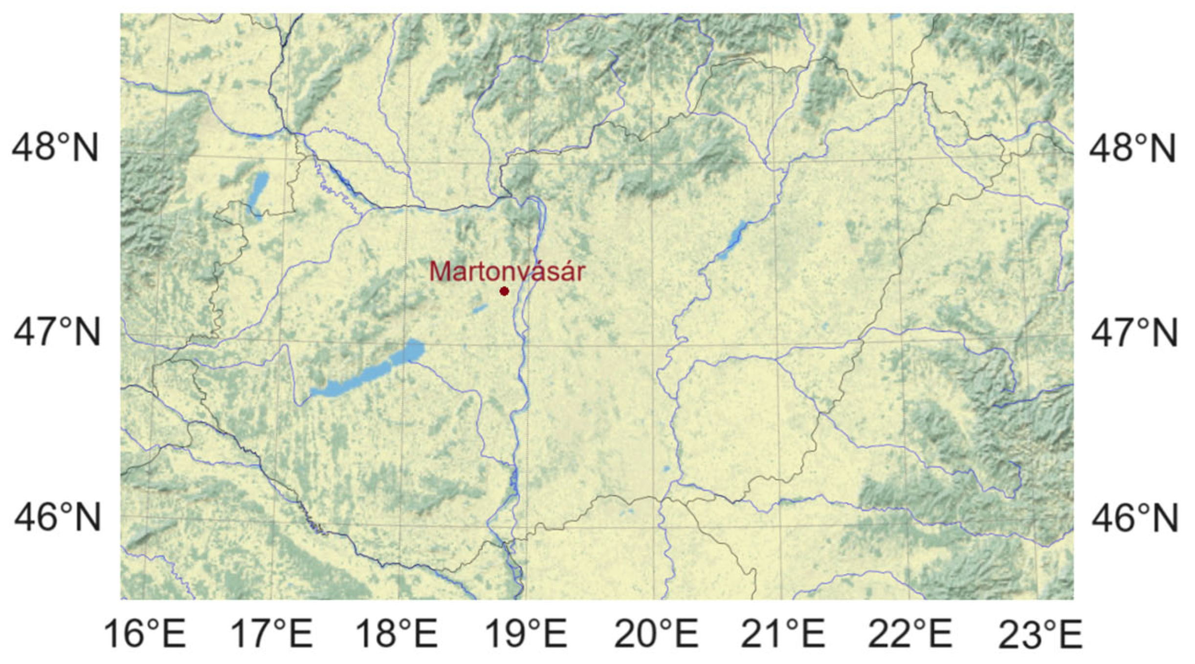
2.2. Location
2.3. Data
2.3.1. Human Data
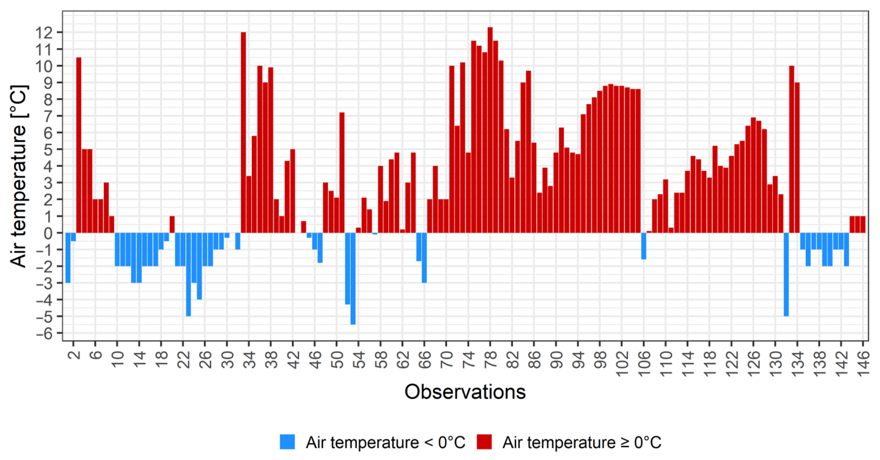
2.3.2. Weather Data
3. Results
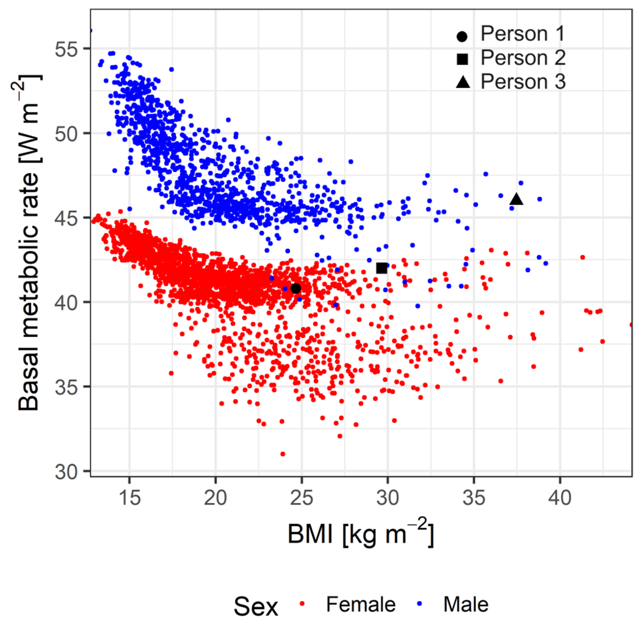
3.1. The Mb–BMI Relationships
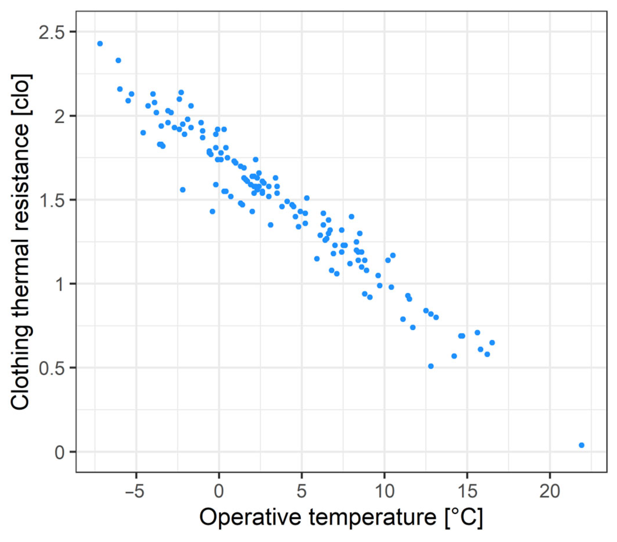
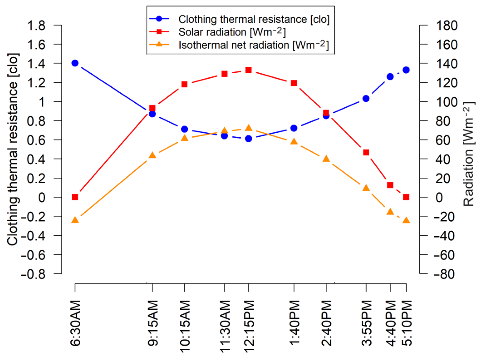
3.2. Clothing Thermal Resistance and Operative Temperature Values Observed in the Fog
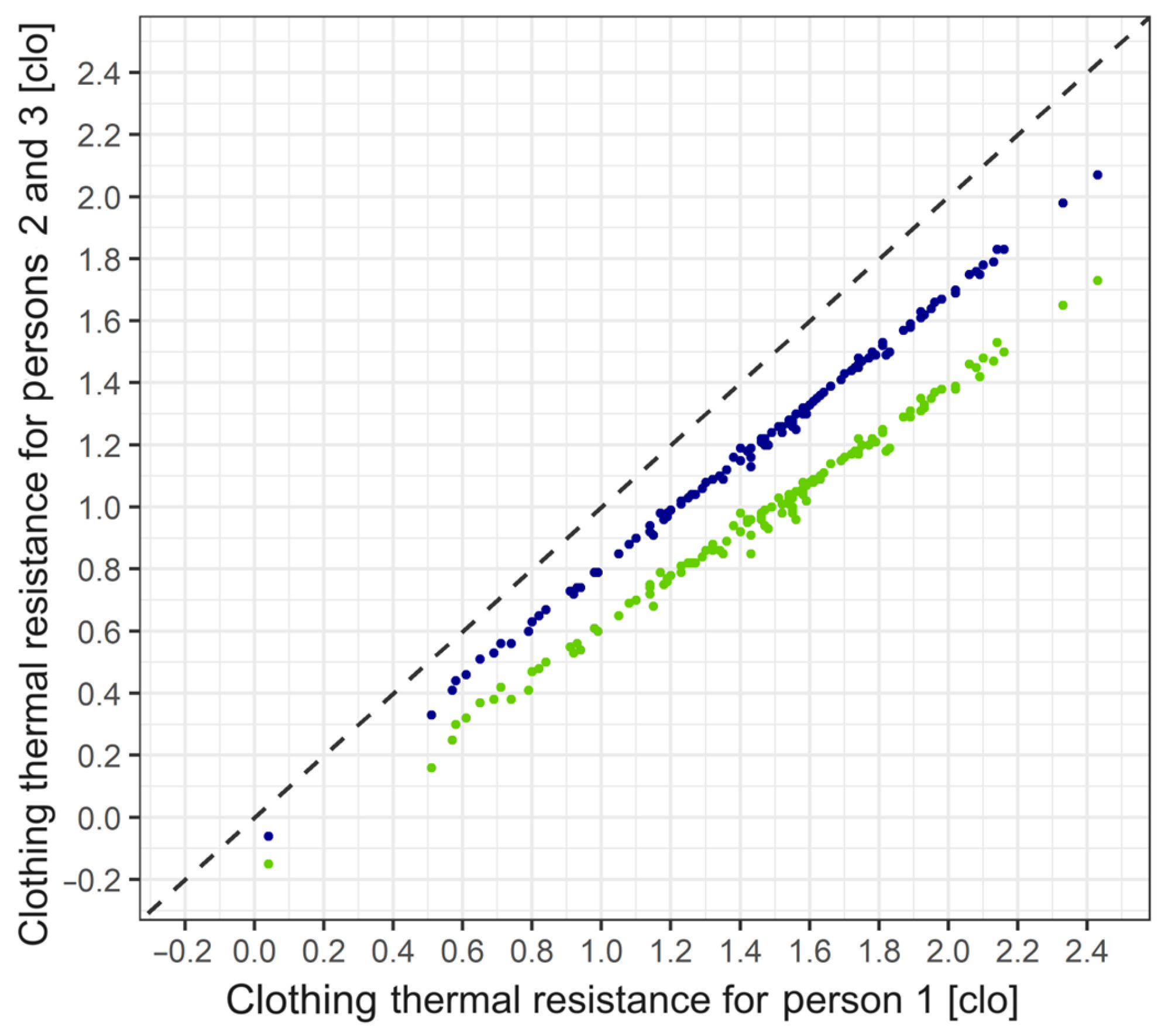
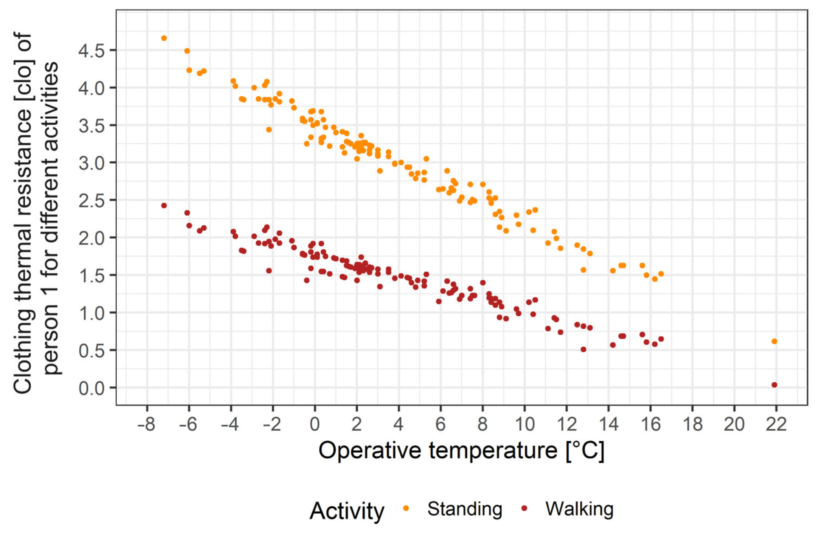
3.3. Sensitivity to Human Factors
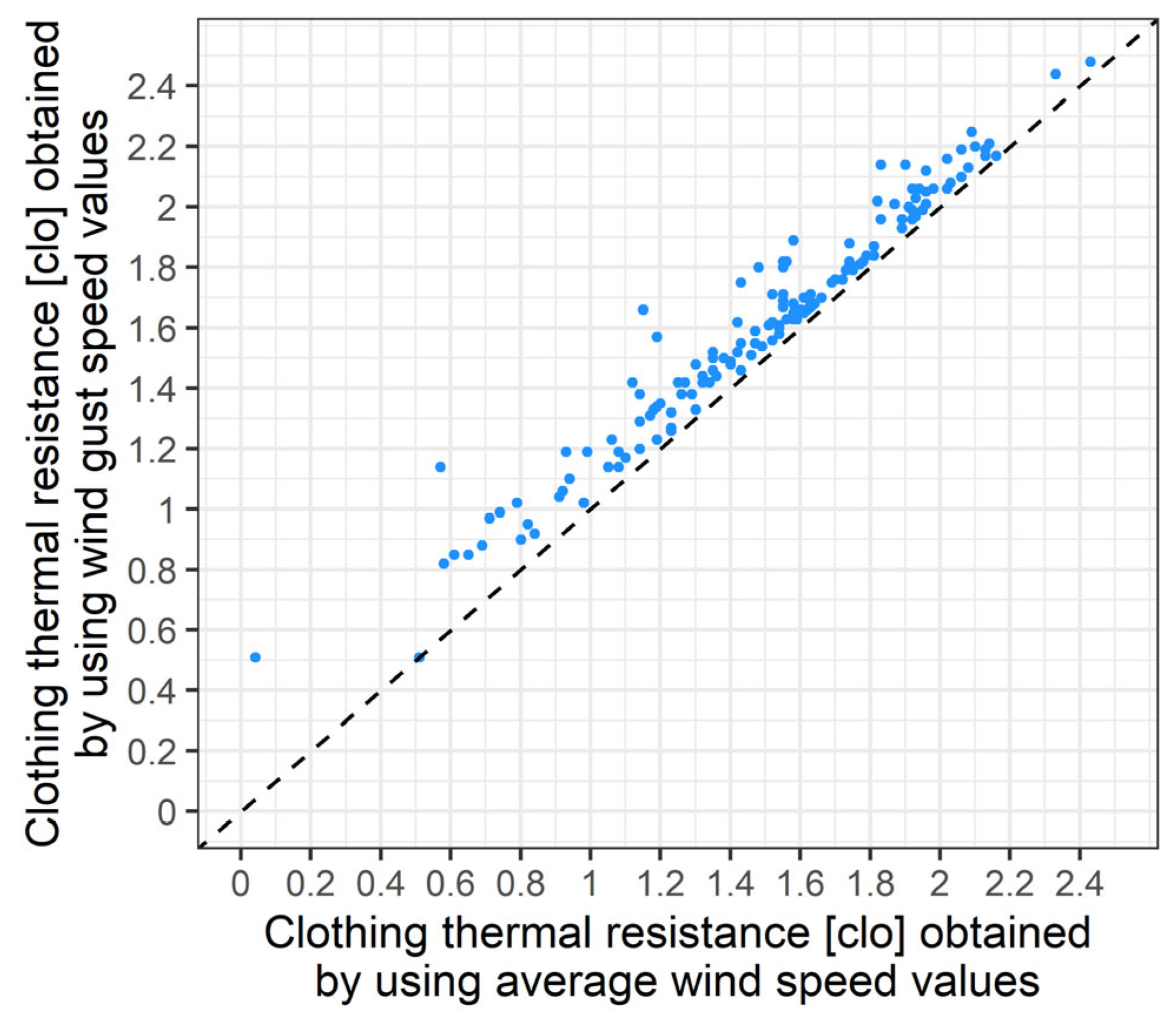
3.4. Sensitivity to Wind Speed
4. Discussion
5. Conclusions
Supplementary Materials
Author Contributions
Funding
Data Availability Statement
Conflicts of Interest
References
- Antal, E. The frequency of fog and its duration in different macrosynoptic situations (A köd gyakorisága és tartama a különböző makroszinoptikus helyzetekben in Hungarian). Időjárás 1958, 62, 39–45. [Google Scholar]
- Kéri, M. The reflection of the metropolitan character in Budapest’s foggy conditions (A nagyvárosi jelleg tükröződése Budapest ködviszonyaiban in Hungarian). Időjárás 1965, 69, 265–270. [Google Scholar]
- Cséplő, A.; Sarkadi, N.; Horváth, Á.; Schmeller, G.; Lemler, T. Fog climatology in Hungary. Időjárás 2019, 123, 241–264. [Google Scholar] [CrossRef]
- Bendix, J. Fog climatology of the Po Valley. Riv. Meteorol. Aeronaut. 1994, 54, 25–36. [Google Scholar]
- Cermak, J.; Eastman, R.M.; Bendix, J.; Warren, S.G. European climatology of fog and low stratus based on geostationary satellite observations. Q. J. R. Meteorol. Soc. 2009, 135, 2125–2130. [Google Scholar] [CrossRef]
- Egli, S.; Thies, B.; Drönner, J.; Cermak, J.; Bendix, J. A 10 year fog and low stratus climatology for Europe based on Meteosat Second Generation data. Q. J. R. Meteorol. Soc. 2017, 143, 530–541. [Google Scholar] [CrossRef]
- Mensbrugghe, V. The formation of fog and of clouds, translated from Ciel et Terre. Symons’s Mon. Meteor. Mag. 1892, 27, 40–41. [Google Scholar]
- Weinstein, A.I.; Silverman, B.A. A numerical analysis of some practical aspects of airborne urea seeding for warm fog dispersal at airports. J. Appl. Meteorol. 1973, 12, 771–780. [Google Scholar] [CrossRef]
- Wantuch, F. Visibility and fog forecasting based on decision tree method. Időjárás 2001, 105, 29–38. [Google Scholar]
- Wu, Y.; Abdel-Aty, M.; Lee, J. Crash risk analysis during fog conditions using real-time traffic data. Accid. Anal. Prev. 2018, 114, 4–11. [Google Scholar] [CrossRef]
- Zhu, Y.; Li, Z.; Zu, F.; Wang, H.; Liu, Q.; Qi, M.; Wang, Y. The propagation of fog and its related pollutants in the Central and Eastern China in winter. Atmos. Res. 2022, 265, 105914. [Google Scholar] [CrossRef]
- Katić, K.; Li, R.; Zeiler, W. Thermophysiological models and their applications: A review. Build. Environ. 2016, 106, 286–300. [Google Scholar] [CrossRef]
- Mayer, H.; Höppe, P.R. Thermal comfort of man in different urban environments. Theor. Appl. Climatol. 1987, 38, 43–49. [Google Scholar] [CrossRef]
- Fröhlich, D.; Matzarakis, A. Modeling of changes in thermal bioclimate: Examples based on urban spaces in Freiburg, Germany. Theor. Appl. Climatol. 2013, 111, 547–558. [Google Scholar] [CrossRef]
- Bröde, P.; Krüger, E.L.; Fiala, D. UTCI: Validation and practical application to the assessment of urban outdoor thermal comfort. Geogr. Pol. 2013, 86, 11–20. [Google Scholar] [CrossRef]
- Schär, C.; Vidale, P.L.; Lüthi, D.; Frei, C.; Häberli, C.; Liniger, M.A.; Appenzeller, C. The role of increasing temperature variability in European summer heatwaves. Nature 2004, 427, 332–336. [Google Scholar] [CrossRef]
- Matzarakis, A.; Mayer, H. Another kind of environmental stress: Thermal stress. WHO Newsl. 1996, 18, 7–10. [Google Scholar]
- Matzarakis, A.; Mayer, H. Heat stress in Greece. Int. J. Biometeorol. 1997, 41, 34–39. [Google Scholar] [CrossRef]
- Potchter, O.; Cohen, P.; Lin, T.P.; Matzarakis, A. Outdoor human thermal perception in various climates: A comprehensive review of approaches, methods and quantification. Sci. Total Environ. 2018, 631–632, 390–406. [Google Scholar] [CrossRef]
- Höppe, P. The Energy Balance in Humans (Original Title—Die Energiebilanz des Menschen); Universitat Munchen, Meteorologisches Institut: Munich, Germany, 1984. [Google Scholar]
- Matzarakis, A.; Mayer, H.; Iziomon, M.G. Applications of a universal thermal index: Physiological equivalent temperature. Int. J. Biometeorol. 1999, 43, 76–84. [Google Scholar] [CrossRef]
- Matzarakis, A.; Rutz, F.; Mayer, H. Modelling radiation fluxes in simple and complex environments—Application of the RayMan model. Int. J. Biometeorol. 2007, 51, 323–334. [Google Scholar] [CrossRef]
- Fiala, D.; Havenith, G.; Bröde, P.; Kampmann, B.; Jendritzky, G. UTCI–Fiala multi-node model of human heat transfer and temperature regulation. Int. J. Biometeorol. 2011, 56, 429–441. [Google Scholar] [CrossRef]
- Havenith, G.; Fiala, D.; Blazejczyk, K.; Richards, M.; Bröde, P.; Holmér, I.; Rintamaki, H.; Benshabat, Y.; Jendritzky, G. The UTCI-clothing model. Int. J. Biometeorol. 2012, 56, 461–470. [Google Scholar] [CrossRef]
- Bröde, P.; Fiala, D.; Blazejczyk, K.; Holmér, I.; Jendritzky, G.; Kampmann, B.; Tinz, B.; Havenith, G. Deriving the operational procedure for the Universal Thermal Climate Index (UTCI). Int. J. Biometeorol. 2012, 56, 481–494. [Google Scholar] [CrossRef]
- Błażejczyk, K.; Twardosz, R. Secular changes (1826–2021) of human thermal stress according to UTCI in Kraków (southern Poland). Int. J. Climatol. 2023, 43, 4220–4230. [Google Scholar] [CrossRef]
- Höppe, P. The physiological equivalent temperature—A universal index for the biometeorological assessment of the thermal environment. Int. J. Biometeorol. 1999, 43, 71–75. [Google Scholar] [CrossRef]
- Ács, F.; Szalkai, Z.; Kristóf, E.; Zsákai, A. Thermal Resistance of Clothing in Human Biometeorological Models. Geogr. Pannonica 2023, 27, 83–90. [Google Scholar] [CrossRef]
- Ács, F.; Zsákai, A.; Kristóf, E.; Szabó, A.I.; Breuer, H. Human thermal climate of the Carpathian Basin. Int. J. Climatol. 2021, 41, E1846–E1859. [Google Scholar] [CrossRef]
- Ács, F.; Kristóf, E.; Zsákai, A. Individual local human thermal climates in the Hungarian lowland: Estimations by a simple clothing resistance-operative temperature model. Int. J. Climatol. 2023, 43, 1273–1292. [Google Scholar] [CrossRef]
- Auliciems, A.; de Freitas, C.R. Cold stress in Canada. A human climatic classification. Int. J. Biometeorol. 1976, 20, 287–294. [Google Scholar] [CrossRef]
- Auliciems, A.; Kalma, J.D. A Climatic Classification of Human Thermal Stress in Australia. J. Appl. Meteorol. 1979, 18, 616–626. [Google Scholar] [CrossRef]
- Yan, Y.Y. Climate Comfort Indices. In Encyclopedia of World Climatology; Oliver, J.E., Ed.; Springer: Dordrecht, The Netherlands, 2005; pp. 227–231. [Google Scholar] [CrossRef]
- Yan, Y.Y.; Oliver, J.E. The Clo: A Utilitarian Unit to Measure Weather/Climate Comfort. Int. J. Climatol. 1996, 16, 1045–1056. [Google Scholar] [CrossRef]
- Campbell, G.S.; Norman, J. An Introduction to Environmental Biophysics, 2nd ed.; Springer: New York, NY, USA, 1997; ISBN 978-0-387-94937-6. [Google Scholar]
- Fanger, P.O. Thermal comfort. In Analysis and Applications in Environmental Engineering; Danish Technical Press: Copenhagen, Denmark, 1970. [Google Scholar]
- Weyand, P.G.; Smith, B.R.; Puyau, M.R.; Butte, N.F. The mass-specific energy cost of human walking is set by stature. J. Exp. Biol. 2010, 213, 3972–3979. [Google Scholar] [CrossRef] [PubMed]
- Frankenfield, D.; Roth-Yousey, L.; Compher, C. Comparison of Predictive Equations for Resting Metabolic Rate in Healthy Nonobese and Obese Adults: A Systematic Review. J. Am. Diet. Assoc. 2005, 105, 775–789. [Google Scholar] [CrossRef] [PubMed]
- Mifflin, M.D.; St Jeor, S.T.; Hill, L.A.; Scott, B.J.; Daugherty, S.A.; Koh, Y.O. A new predictive equation for resting energy expenditure in healthy individuals. Am. J. Clin. Nutr. 1990, 51, 241–247. [Google Scholar] [CrossRef]
- Dubois, D.; Dubois, E.F. The Measurement of the Surface Area of Man. Arch. Intern. Med. 1915, 15, 868–881. [Google Scholar] [CrossRef]
- Thermal Comfort. Innova Air Tech Instruments A/S. 2002. Available online: http://www.labeee.ufsc.br/sites/default/files/disciplinas/Thermal%20Booklet.pdf (accessed on 2 February 2024).
- Mihailović, D.T.; Ács, F. Calculation of daily amounts of global radiation in Novi Sad. Időjárás 1985, 89, 257–261. (In Hungarian) [Google Scholar]
- Brunt, D. Notes on radiation in the atmosphere. Q. J. R. Meteorol. Soc. 1932, 58, 389–420. [Google Scholar] [CrossRef]
- Konzelmann, T.; van de Wal, R.S.W.; Greuell, W.; Bintanja, R.; Henneken, E.A.C.; Abe-Ouchi, A. Parameterization of global and longwave incoming radiation for the Greenland Ice Sheet. Glob. Planet. Chang. 1994, 9, 143–164. [Google Scholar] [CrossRef]
- Ács, F.; Breuer, H.; Skarbit, N. Climate of Hungary in the twentieth century according to Feddema. Theor. Appl. Climatol. 2015, 119, 161–169. [Google Scholar] [CrossRef]
- Ács, F.; Kristóf, E.; Szabó, A.I.; Zsákai, A. New statistical deterministic method for estimating human thermal load and sensation—Application in the Carpathian region. Theor. Appl. Climatol. 2023, 151, 691–705. [Google Scholar] [CrossRef]
- Utczás, K.; Zsákai, A.; Muzsnai, Á.; Fehér, V.P.; Bodzsár, É. The analysis of bone age estimations performed by radiological and ultrasonic methods in children aged between 7–17 years (Radiológiai és ultrahangos módszerrel végzett csontéletkor-becslések összehasonlító elemzése 7–17 éveseknél in Hungarian). Anthrop. Közl. 2015, 56, 129–138. [Google Scholar] [CrossRef]
- Zsákai, A.; Bodzsár, É. The relationship between reproductive ageing and the changes of bone structure in women (A reprodukciós öregedés és csontszerkezet változásának kapcsolata nőknél in Hungarian). Anthrop. Közl. 2016, 57, 77–84. [Google Scholar] [CrossRef]
- Fehér, V.P.; Annár, D.; Zsákai, A.; Bodzsár, É. The determinants of psychosomatic health complaints in 18–90 year-old women (Pszichoszomatikus tünetek gyakoriságát befolyásoló tényezők 18–90 éves nők körében in Hungarian). Anthrop. Közl. 2019, 60, 65–77. [Google Scholar] [CrossRef]
- Di Napoli, C.; Pappenberger, F.; Cloke, H.L. Assessing heat-related health risk in Europe via the Universal Thermal Climate Index (UTCI). Int. J. Biometeorol. 2018, 62, 1155–1165. [Google Scholar] [CrossRef]
- Amaro-Gahete, F.J.; Sanchez-Delgado, G.; Alcantara, J.M.A.; Martinez-Tellez, B.; Acosta, F.M.; Merchan-Ramirez, E.; Löf, M.; Labayen, I.; Ruiz, J.R. Energy expenditure differences across lying, sitting, and standing positions in young healthy adults. PLoS ONE 2019, 14, e0217029. [Google Scholar] [CrossRef]
- Júdice, P.B.; Hamilton, M.T.; Sardinha, L.B.; Zderic, T.W.; Silva, A.M. What is the metabolic and energy cost of sitting, standing and sit/stand transitions? Eur. J. Appl. Physiol. 2016, 116, 263–273. [Google Scholar] [CrossRef] [PubMed]
- Bašarin, B.; Lukić, T.; Matzarakis, A. Review of Biometeorology of Heatwaves and Warm Extremes in Europe. Atmosphere 2020, 11, 1276. [Google Scholar] [CrossRef]
- Köppe, C.; Kovats, S.; Jendritzky, G.; Menne, B. Heat Waves: Risks and Responses, No. 2; Health and Global Environmental Change Series; World Health Organisation: Copenhagen, Denmark, 2004. [Google Scholar]
- Holmér, I. Assessment of cold stress in terms of required clothing insulation—IREQ. Int. J. Ind. Ergon. 1988, 3, 159–166. [Google Scholar] [CrossRef]
- Kuchcik, M.; Blažejczyk, K.; Halaś, A. Long-term changes in hazardous heat and cold stress in humans: Multicity study in Poland. Int. J. Biometeorol. 2021, 65, 1567–1578. [Google Scholar] [CrossRef] [PubMed]
- Nastos, P.T.; Matzarakis, A. The effect of air temperature and human thermal indices on mortality in Athens, Greece. Theor. Appl. Climatol. 2012, 108, 591–599. [Google Scholar] [CrossRef]
- Błażejczyk, A.; Błażejczyk, K.; Baranowski, J.; Kuchcik, M. Heat stress mortality and desired adaption responses of healthcare system in Poland. Int. J. Biometeorol. 2018, 62, 307–318. [Google Scholar] [CrossRef] [PubMed]
- Błażejczyk, K.; Kunert, A. Bioclimatic Principles of Recreation and Tourism in Poland (Bioklimatyczne Uwarunkowania Rekreacji i Turystyki w Polsce in Polish); Polish Academy of Sciences S. Leszczycki Institute of Geography and Spatial Organization: Warsaw, Poland, 2011; p. 365. [Google Scholar]


| Person | Sex | Age [Years] | Body Mass [kg] | Body Length [cm] | Basal Metabolic Heat Flux Density [W m−2] |
|---|---|---|---|---|---|
| person 1 | male | 68 | 89 | 190 | 39.56 |
| person 2 | male | 53 | 95 | 179 | 41.81 |
| person 3 | male | 24 | 120 | 179 | 45.93 |
Disclaimer/Publisher’s Note: The statements, opinions and data contained in all publications are solely those of the individual author(s) and contributor(s) and not of MDPI and/or the editor(s). MDPI and/or the editor(s) disclaim responsibility for any injury to people or property resulting from any ideas, methods, instructions or products referred to in the content. |
© 2024 by the authors. Licensee MDPI, Basel, Switzerland. This article is an open access article distributed under the terms and conditions of the Creative Commons Attribution (CC BY) license (https://creativecommons.org/licenses/by/4.0/).
Share and Cite
Kristóf, E.; Ács, F.; Zsákai, A. On the Human Thermal Load in Fog. Meteorology 2024, 3, 83-96. https://doi.org/10.3390/meteorology3010004
Kristóf E, Ács F, Zsákai A. On the Human Thermal Load in Fog. Meteorology. 2024; 3(1):83-96. https://doi.org/10.3390/meteorology3010004
Chicago/Turabian StyleKristóf, Erzsébet, Ferenc Ács, and Annamária Zsákai. 2024. "On the Human Thermal Load in Fog" Meteorology 3, no. 1: 83-96. https://doi.org/10.3390/meteorology3010004