A Wind Field Reconstruction from Numerical Weather Prediction Data Based on a Meteo Particle Model

Abstract

In the present work, a methodology for wind field reconstruction based on the Meteo Particle model (MPM) from numerical weather prediction (NWP) data is presented. The development of specific wind forecast services is a challenging research topic, in particular for what concerns the availability of accurate local weather forecasts in highly populated areas. Currently, even if NWP limited area models (LAMs) are run at a spatial resolution of about 1 km, this level of information is not sufficient for many applications; for example, to support drone operation in urban contexts. The coupling of the MPM with the NWP limited area model COSMO has been implemented in such a way that the MPM reads the NWP output over a selected area and provides wind values for the generic point considered for the investigation. The numerical results obtained reveal the good behavior of the method in reproducing the general trend of the wind speed, as also confirmed by the power spectra analysis. The MPM is able to step over the intrinsic limitations of the NWP model in terms of the spatial and temporal resolution, even if the MPM inherits the bias that inevitably affects the COSMO output.

1. Introduction

The need for accurate wind prediction is particularly felt in many application fields. Wind turbines need to be strategically placed to capture as much energy as possible, since the amount of power that can be harnessed from the wind is directly proportional to its speed. Thunderstorms, tornadoes, and hurricanes are characterized by strong winds that can cause injury and damage to critical facilities. It is well known that small drones are vulnerable to the action of winds, especially at low altitudes. Areas with high wind are considered as hazards for drones, since they cannot be visually detected by the pilot or detected by sensors [1]. For this reason, the development of specific forecast services is a challenging research topic, in particular for what concerns the availability of accurate local weather forecasts in highly populated areas. In this view, the SESAR U-SPACE program [2] was established in order to develop a UTM (Unmanned Traffic Management) system with an advanced introduction of procedures and services designed to support efficient and protected access to the airspace for a high number of drones.

In the last decade, several methodologies for the estimation of winds at low altitudes in urban areas have been developed. Some of them were originally developed for reconstruction at high altitudes and successively adapted to treat different heights. Statistical data and techniques based on the Kalman filter [3] were used in Ref. [4] to estimate the wind values aimed to the trajectory definition. In 2014, de Jong et al. [5] introduced the AWEA (airborne wind-estimation algorithm) algorithm based on the fact that aircrafts are equipped with automatic systems (e.g., ADS-B [6]) for atmospheric data, permitting the reception of information from vehicles in proximity and providing high-fidelity and high-resolution user-tailored wind profiles. Recently, Kiessling et al. [7] developed the random Fourier features, a novel interpolation model based on a machine-learning approach, resulting in a competitive model with respect to other statistical interpolation models, such as kriging or other machine-learning methods, e.g., random forests and neural networks. In 2018, Sun et al. [8] introduced the Meteo Particle Model (MPM), aimed at providing an estimate of atmospheric variables inside the airspace using surveillance data from aircrafts. This model is based on the usage of a stochastic process to obtain weather information (wind and temperature) in a short time range (less than 24 h) in areas where observations are lacking, starting from the data collected along high-density flight trajectories. Variables are reconstructed using virtual particles that are generated every time new observations are available. Successively, in the frame of the METSIS project [9], Sunil et al. extended the MPM to low altitudes, evaluating the wind fields over an area of about 3600 m² by using a Monte Carlo approach and assuming that they were pseudostatic on a short time scale, thus being able to consider the effects of the presence of obstacles (trees, buildings). The applicability of the MPM at different altitudes was investigated by Zhu et al. [10] over an area of 600 km in diameter. In Ref. [11], Bucchignani analyzed the main methodologies used to estimate low-altitude winds in urban areas. The most promising technique among those examined was the one based on the MPM due to its flexibility features and the accuracy in the results obtained: in fact, the MPM was able to address the random characteristics of the wind through particles and preserved the stability through the use of a large number of particles.

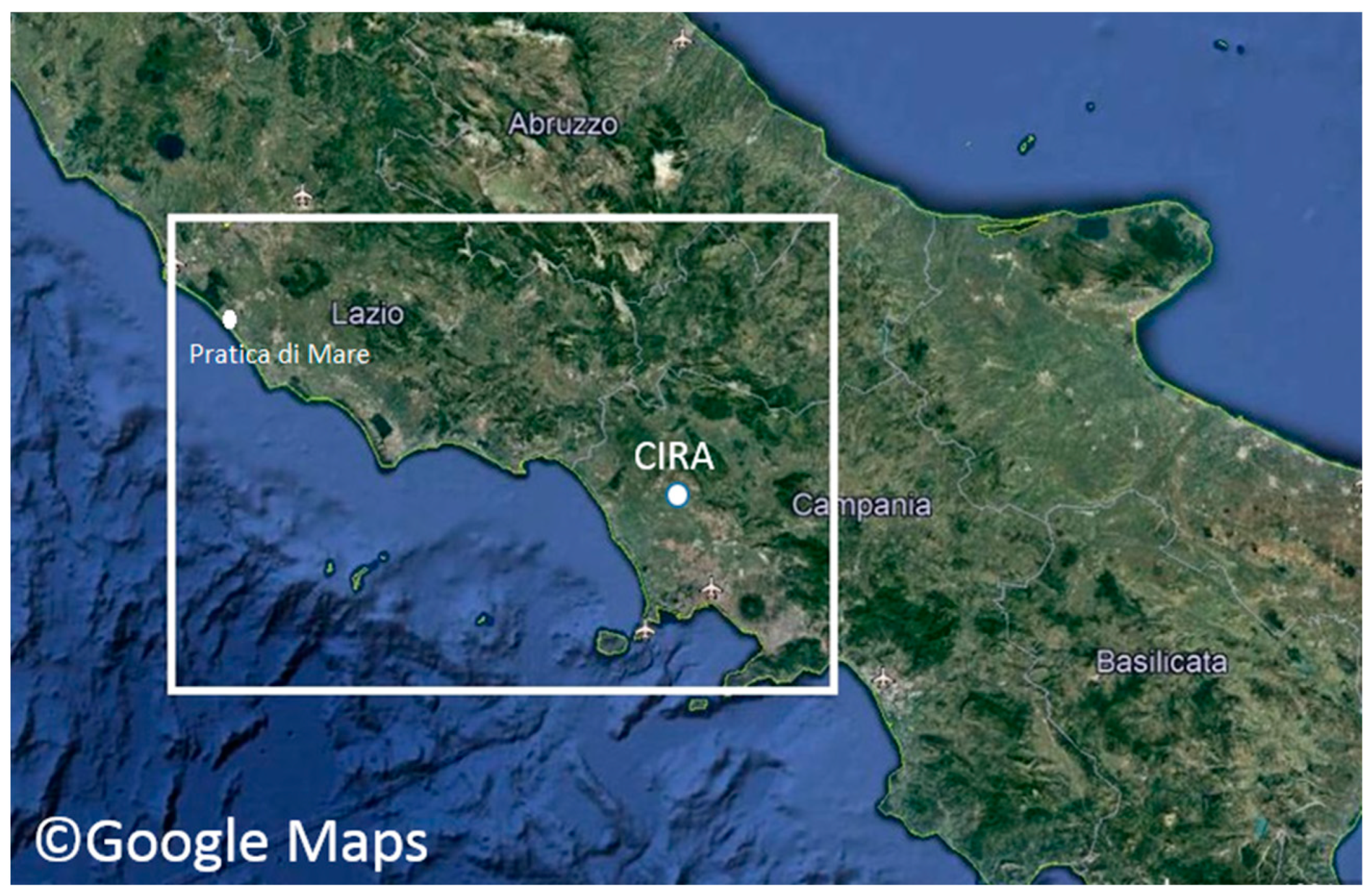
At the Italian Aerospace Research Center (CIRA, Italy), an operational platform HW/SW is currently available, made up of a ground element (the Meteo Service Center) that, through MATISSE software version 1 [12], collects, processes, and prepares observational and atmospheric forecast data (in different time ranges). Numerical forecasts are taken from the operational prediction system COSMO [13] and the new-generation system ICON [14]: a configuration for these models at a resolution of about 1 km, including urban parameterizations for a proper representation of the subdaily dynamic behavior in urban areas, has been developed over an area located in southern Italy. Moreover, CIRA is carrying out the EDUS project, “Infrastrutture di elaborazione dati locali per U-SPACE”, aimed to enhance the Meteo Service Center in order to integrate data and algorithms with newer ones suitable for the treatment of urban wind. However, limitations in the applications of the reconstruction methodologies for wind fields are related to the fact that reliable estimations can be produced only if a sufficient number of drones are already flying in the area considered and/or if a sufficient number of weather stations are available; this limitation can be mitigated by using the data provided by NWPs. In fact, as stated in Ref. [11], a step forward would be represented by the coupling of an NWP model with the MPM due to the feasibility of the MPM and the accuracy in the results obtained with this model. Currently, even if the NWP limited area models (LAMs) are run at a spatial resolution of about 1 km (thanks to the growth of computational resources), this level of information is still not sufficient to support drone operation in urban contexts. For this reason, further enhancements are still needed, as discussed in the present work. The proposed coupling will ensure that estimations can be generated in any geographical area, not only where an adequate number of drones are already flying. It is worth noting that this approach for low-altitude wind reconstruction could also be applied to other practical applications, like utility-scale wind turbine applications [15,16]. The main aim of this work is the presentation of this coupled system, along with the verification of its capabilities over a selected test case. This paper is organized as follows: Section 2 contains a description of the MPM. Section 3 describes examples of MPM applications reported in the literature. Section 4 contains a description of the adopted NWP model and observational data. The methodology is described in Section 5, while, in Section 6, the main results are presented. Conclusions are then discussed in Section 7.

2. The Meteo Particle Model

For the wind field reconstruction, inversion methods were employed to estimate the characteristics of the atmospheric or wind conditions based on the data collected from various sources. These methods typically involve solving mathematical equations or optimization problems to find the most likely set of parameters that would explain the observed data. Then, observations were integrated into the inversion process, adjusting the model parameters to best match the real-world observations. Finally, the reliability and accuracy of the inversion results were assessed, as well as the results of the variations in the input data and model assumptions. The Meteo Particle Model was developed by Sun et al. [8] with the aim of providing a reconstruction of the atmospheric variables inside the airspace using only surveillance data from aircrafts. The method is exhaustively described in [8,9], and also summarized in Ref. [11], so only the main steps are recalled here.

2.1. Selection of the Input Data

A reference domain D was chosen, in which periodic measurements were available from aircrafts or drones flying inside it. The measurements performed by the different aircrafts were collected and stored in a specific measurement array; then, a probabilistic selection process was adopted to remove the incorrect measurements that could occur. In this way, the data related to extreme values had a low probability of being selected. A Gaussian probabilistic function was defined, starting from the current observations (array x), once the mean μ and variance σ were calculated:

$$p=\exp \left[-\frac{1}{2}\frac{{\left(x-\mu \right)}^T(x-\mu )}{k_1\sigma }\right]$$

in which k₁ is a control parameter defined as an acceptance probability factor. The numerical value k₁ is defined in an empirical way, and its value can be augmented to allow for a larger tolerance (an increase in the number of accepted measurements). The authors of the method proposed to assign the value 3 to this parameter.

2.2. Construction of the Particles

The method is based on the idea of using “particles”, which are virtual objects able to carry information on the state of the wind and temperature. Specifically, N particles (the integer number N is selected by the user according to specific needs) were generated, close to the position of the aircraft that performed the evaluation, every time new measurements were available. Successively, the method assumes that the particles move according to a Gaussian random walk model in the horizontal direction, while, along the vertical direction, the motion follows a zero-average Gaussian track. The particles with a motion that fell outside of the domain were removed, while the remaining ones were classified according to their age, which was set as equal to zero at the time of the initialization, and which increased in the successive steps.

2.3. Evaluation of the Variable Values at a Generic Point

The main aim of the method was the evaluation of the values of the wind components u, v, and w at a generic point of the domain D. This can be achieved as a weighted average of the values carried by the particles, belonging to an ensemble p which includes all the particles and whose coordinates are within a maximum distance from the coordinates of the position being considered:

$$u\left(x,y,z\right)={\sum }_i{W}_{p,i}{u}_{p,i}$$

$$v\left(x,y,z\right)={\sum }_i{W}_{p,i}{v}_{p,i}$$

$$w\left(x,y,z\right)=\sum _i{W}_{p,i}{w}_{p,i}$$

in which u_pi, v_pi, and w_pi are the velocity components of the i-th particle. The previous sums are extended to all the particles of the p ensemble.

The weight W assigned to each particle is calculated as a product of two exponential functions: the first one represents a relationship between the weight itself and the distance d between the particle and the position considered, while the second one establishes a relation between the weight and the distance d₀ of the particle from its origin:

$$W_p=f_d\left(d\right)·f_0\left(d_0\right)$$

$$f_d(d)=\mathrm{e}\mathrm{x}\mathrm{p} [-\frac{{\left(d\right)}^2}{2C_d^2}]$$

$$f_0(d_0)=\mathrm{e}\mathrm{x}\mathrm{p} [-\frac{{\left(d_0\right)}^2}{2C_d^2}]$$

in which C_d is a weighting parameter. These formulae are based on the IDV technique (inverse distance-weighted) [17]. The MPM does not use a predefined grid, but the numerical values can be calculated at a generic point provided that a sufficient number of particles are present close to the point.

3. MPM: Examples of Practical Applications

The MPM has been used for practical applications in several contexts. In the frame of the METSIS project (METeo Sensors In the Sky) [9], the model was used to support the wind nowcasting inside the U-SPACE Weather Information Service. Specifically, wind data were generated in the area considered, starting from the measurements performed by the drones themselves; the data were then provided to the drone operators by using the mentioned information service. The evaluation of the accuracy of the wind estimations was carried out through a series of experiments, and presented by Sunil et al. in Ref. [9]. Three measurement drones were used to collect the data needed by the MPM, located in such a way as to form an equilateral triangle, while a reference drone was used to determine the accuracy of the methodology. A parametric analysis was conducted by varying the size of the triangle and the altitude, and by considering the presence of different obstacles (no obstacle, a trailer, a tree). The results showed that the performances for the wind speed in terms of the mean absolute error (MAE) were satisfactory, with a larger MAE for the scenario including an obstacle. The accuracy for the direction was rather scarce, especially for smaller wind speeds.

The MPM was used by Sun et al. [18] for the reconstruction of wind fields, starting from observational data from the ADS-B [6] (an aviation surveillance technology, in which an aircraft determines its position via satellite navigation, such as GNSS or other sensors) and Mode-S [19] for an area located in the vicinity of Delft, about 600 km in diameter. The model was validated by using the data provided by the analyses of the GFS meteorological model [20] for one week, starting on 27 July 2017. It was found that, for a low wind speed, the results were less aligned with the reference data. This inaccuracy could be due to the fact that the GFS data were interpolated and smoothed over larger periods of time and areas. Moreover, it was found that the correctness of the results was largely influenced by the input data accuracy.

Finally, Zhu et al. [10] investigated the applicability of the method to different levels of altitude, considering the same area as used by Sun et al. [18]. The accuracy of the MPM was evaluated against the ERA-5 reanalysis [21] at a resolution of 0.25°. It was found that the MAE speed error increased with the altitude (from 1 m/s at 1 km to 8 m/s at 12 km), while the MAE was related to direction ranges between 4 and 14°.

4. The NWP Model and Observational Data

4.1. The LAM COSMO Model

Scientific and technological progress has led to an increase in the capabilities of weather forecasting over the past 40 years. Mazzarella et al. [22] investigated whether NWP-based weather forecasts at a high-resolution (including data assimilation) could improve the capability of the prediction of extreme events in order to understand if such models could be suitable for supporting air traffic management. They found that, for a specific test case, the model was able to provide forecasts at least 1 h in advance, giving ATM operators sufficient time to manage air traffic and calculate new landing trajectories prior to an extreme event. In the present work, the MPM model was coupled with the limited-area model COSMO [13], which is a nonhydrostatic dynamic downscaling model for three-dimensional compressible flows developed by the European consortium COSMO (COnsortium for Small-scale MOdeling). This model treats the atmosphere as an ideal mixture of dry air, water vapor, and liquid and solid water subject to gravity and to Coriolis forces [23]. A convective-scale model configuration characterized by a horizontal resolution of about 1 km was developed at CIRA, and is running daily over an area (12.22–14.55° E; 40.63–41.88° N) (Figure 1) located in southern Italy. The computational domain has 260 × 138 points, while the number of vertical levels is set as equal to 60. The time step is set as equal to 10 s. The initial and boundary conditions are provided by the ECMWF IFS global model [24] at a spatial resolution of 0.075°.

The capabilities of the COSMO model in simulating the main atmospheric variables over this domain have already been tested against the data provided by the CIRA weather instrumentation and other data, and the results were presented in [25]. In particular, the wind values were validated against the data provided by the wind profiler installed at CIRA (owned by ARPAC—Environmental Protection Agency of Campania Region), revealing the good model performance and suggesting the great potential of the model to support forecasts for drone flights.

For the purposes of the present work, the COSMO output data over a 10 km × 10 km subgrid have been extracted for the MPM application, whose size appears to be reasonable for a drone flight area. This subgrid is centered over the target point located at the CIRA facilities (14.160 E; 41.120 N) (shown in Figure 1). The original coordinate values in degrees have been converted into meters, assuming the bottom-left point of the subgrid as the origin (0,0).

4.2. Observational Data

The model evaluation was conducted using 10 m wind values provided by two weather stations, MAWS301, installed at CIRA. They were produced by Vaisala, powered by photovoltaic panels, and equipped with a 12 V/27 Ah buffer battery. Specifically, Weather Station 1 is equipped with various sensors for measuring several atmospheric variables, while Weather Station 2 is only equipped with an anemometer for measuring the wind at 10 m (the direction and intensity). For each of the two weather stations, data reception occurs via a data logger positioned at the base of the pole, which communicates via a radio-modem with an antenna positioned on the roof of the CIRA main building in line of sight with the two transmitting antennas. These communications take place in UHF, and the frequency used is set at 395 MHz. Furthermore, dedicated software automatically creates two text files per day (one for each station), in which all the measurements taken over the course of 24 h are saved, with a time resolution of 1 min.

5. Description of the Methodology

The coupling of the MPM with the LAM COSMO has been realized in such a way that the MPM reads the hourly NWP output at a high resolution over the considered subgrid, generates particles at each grid point, and provides wind values for every minute at the generic point considered for the investigation. Since the observational data are available only at 10 m of height, in the present work, only the 10 m wind velocity provided by COSMO was considered. The tool works through the following steps:

• The daily output NWP files related to a subgrid are read. This subgrid is made up of n × n points (in the present study, n has been set as equal to 10) centered over the location object of the investigation, and contains 24 hourly values of 10 m wind velocity (horizontal u and v components).
• For every 24 h, a family of N particles is generated, which are initially located in the grid points at a height of 10 m (Figure 2a), and which are characterized by a velocity equal to the wind velocity in the corresponding points. The age of this family (α) is initially equal to zero, but at each successive hour, its age is increased by 1 unit.
• For every 60 min of the current hour, the updated position of the particles is calculated, considering their own velocity components, u_i and v_i (with i = 1 … N):

$$x_{p,i,t+∆t}=x_{p,i,t}+∆P_{x,i,t}$$

$$y_{p,i,t+∆t}=y_{p,i,t}+∆P_{y,i,t}$$

in which the ΔP factors are calculated as:

$${∆P}_{x,i,t}=k_2{\sigma u}_i∆t$$

$${∆P}_{y,i,t}=k_2{\sigma v}_i∆t$$

meaning that the particles move according to a random track horizontal motion, characterized by a small bias (σ), conveniently controlled by the k₂ factor (the particle random walk factor), which was originally set as equal to 10 in Ref. [8], but which was modified for other applications (e.g., it was set as equal to 8 in Ref. [10]). The time step Δt is equal to 1 min.

Then, the three particles closest to the target point were individuated by means of exhaustive research, and the provisional velocity at the target point was calculated as the weighted mean of the velocity values of these three particles (Figure 2b). The weight to be assigned to each particle was calculated as a function of the distance of the target point from the particle itself.

• Finally, the velocity in the target point is calculated as the weighted mean among the provisional values associated to the families generated until this point. The weight to be assigned to each provisional value is calculated as a function of the age (α) of the corresponding family:

$$f(\alpha )=\mathrm{e}\mathrm{x}\mathrm{p} [-\frac{{\left(\alpha \right)}^2}{2C_{\alpha }^2}]$$

(1)

where α is a number that represents the age of the particle and C_α is a control parameter (aging parameter) chosen by the user. It could be set as equal to 30, according to the indications of the authors of the method. The algorithm is summarized in Figure 3.

6. Results

The coupled NWP–MPM system was tested for each day of the period from 1 to 30 June 2020, considering three different MPM configurations. Each configuration was characterized by the specific values of the control factors defined in the previous sections, as summarized in

Table 1. Values of the control factors defined in the MPM for the three configurations tested.

Factor	Config 1	Config 2	Config 3
Acceptance probability factor k1	3	4	7
Particle random walk factor k2	10	9	8
Aging parameter C0	30	40	50

. These values were chosen according to the experiments performed and considering the recommendations provided in specific works in the literature. As described later, the first configuration (Config 1) provided the best results, and was selected for a more detailed analysis. Figure 4 shows the position of the first family of particles for 1 June 2020 at (a) the beginning of the simulation at 1:00 a.m. (which is assumed as t = 0) and after (b) 1 min, (c) 2 min, and (d) 10 min, respectively. The velocity vectors that characterize each particle are also shown. The 10 × 10 subgrid extracted from COSMO is visible in Figure 4a: in fact, as already described, at the beginning of the simulation, the position of the particles coincides with those of the grid points. Figure 5 shows the wind field reconstruction performed by the MPM after 1 min in the neighborhood of the target point (5560 m; 4670 m). The wind vectors reconstructed in the sample points at a distance of 100 m between one another in the two directions are represented by red arrows, while the original wind vectors provided by COSMO are represented by black arrows.

Figure 6 shows the time series of the wind speed for the days from 1 to 6 June 2020 provided by the MPM and by the weather station at a frequency of 1 m. The original COSMO data (for the grid point closest to the target one) are also shown (identified by green asterisks), which are available every hour. These plots reveal the good behavior of the MPM in reproducing the general trend of the wind speed over the whole days considered; in particular, the wind increase observed almost every day between 600 and 800 m (i.e., between 11 a.m. and 1 p.m.) is well captured. Non-negligible discrepancies are, however, observed on some days, in particular in the last hours of each simulation, along with some overestimations in the central part of the day, in particular on 1 June 2020. It is worth noting that most of the inaccuracies are inherited by the COSMO model output; however, the MPM is able to overperform the NWP model (see

Table 2. Numerical values of the BIAS and the RMSE of the wind speed (m/s) for the COSMO and MPM for three different configurations with respect to the observations, obtained as average values over the period 1–30 June 2020.

Model	BIAS Speed	Max BIAS Speed	RMSE Speed
COSMO	0.10	0.24	0.46
MPM 1	0.03	0.84	0.37
MPM 2	0.04	0.88	0.39
MPM 3	0.07	0.92	0.52

and

Table 3. Numerical values of the BIAS and the RMSE of the wind direction (°) for the COSMO and MPM for three different configurations with respect to the observations, obtained as average values over the period 1–30 June 2020.

Model	BIAS Direction	Max BIAS Direction	RMS Direction
COSMO	14	81	26
MPM 1	12	72	24
MPM 2	16	68	32
MPM 3	19	88	36

for a detailed comparison), as discussed later. The time series were processed by using an FFT aimed to produce the power spectra of the wind at regularly spaced bins to measure the amount of variability occurring at different frequency bands. Figure 7 shows the mean power spectra (log–log representation) related to the time series of 1 June 2020, related to the observational data (left) and the MPM data (right), respectively. It can be observed that the two spectra appear similar and that the main observed frequency (0.0027, corresponding to a period of 6 h) is well captured by the model.

In order to quantify the model performances, standard indices for the performance evaluation have been calculated: the mean bias (BIAS) and the root mean square error (RMSE), defined as:

$$\mathrm{B}\mathrm{I}\mathrm{A}\mathrm{S}=\frac{1}{N}\sum _{i=1}^N\left(S_i-O_i\right)$$

(2)

$$\mathrm{R}\mathrm{M}\mathrm{S}\mathrm{E}=\sqrt{\frac{1}{N}\sum _{i=1}^N{\left(S_i-O_i\right)}^2}$$

(3)

where S_i and O_i are, respectively, the simulated and observed values at the i-th time step. N is the number of time steps considered (1440 for each day).

Table 2 shows the numerical values of these indicators related to the wind speed for the COSMO and MPM (three configurations) with respect to the observations, obtained considering the whole period (1–30 June 2020). Specifically, the BIAS and RMSE speeds are obtained considering the daily values first and then averaging them over the thirty days considered. The max BIAS speed is the maximum value among the thirty daily values. The COSMO grid data for the CIRA position are interpolated by using an ordinary kriging methodology.

The analysis of Table 2 reveals that the best performance of the MPM was obtained with Config 1, and that the MPM was able to overperform the NWP COSMO on average, even if, on some days, the MPM was characterized by larger biases.

Table 3 shows the numerical values of the same indicators related to the wind direction (°) for the COSMO and MPM (three configurations) with respect to the observations over the same period. It can be seen that, even if the model overperformed the COSMO output, the direction accuracy on some days was rather scarce, as also observed in [9], especially at smaller wind speeds.

The World Meteorological Organization (WMO) has provided reference values for the accuracy of the wind measurements, i.e., 0.5 m/s (<5 m/s) and 10% (>5 m/s) for the speed and 5° for the direction [26], implying that the accuracy obtained in the present application is acceptable for the speed, while it should be improved for the direction.

7. Conclusions

In the present work, a methodology for wind field reconstruction based on the Meteo Particle Model from numerical weather prediction data was presented. The problem of wind forecasting is particularly felt for aeronautical applications; in fact, several studies (e.g., [27]) have examined the effect of errors in wind forecasting on continuous descent operations, finding that an accurate knowledge of wind conditions is important, since about 2/3 of the errors are due to an incorrect wind forecast. Moreover, the meteorological conditions in urban environments require detailed analysis because of the influence that the characteristics of the urban fabric can have on local meteorological conditions. The impact can be more or less significant depending on the field of applications. Beyond the applications to drones, the present approach for low-altitude wind reconstruction can also be applied to other cases, e.g., ship–helicopter operational limitation analysis [28], crane safety in the construction industry [29], and as a further input to national meteorological services.

The coupling of the MPM with the LAM COSMO has been implemented in such a way that the MPM reads the NWP output at a high resolution over a selected region and provides wind values for the generic point considered in the investigation. The numerical results obtained revealed the good behavior of the method in reproducing the general trend of the wind speed, as also confirmed by the power spectra analysis. The MPM was able to step over the intrinsic limitations of the NWP model in terms of the spatial and temporal resolution, even if, as expected, the MPM inherited the bias that inevitably affected the COSMO output. For this reason, in the opinion of the author, a step forward will be represented by the application of a bias-correction technique [30] to the NWP output, performed considering a validation period in which observed and modeled time series are available and overlapped. In fact, NWP postprocessing has become a standard practice; for example, by using the model output statistics (MOSs) that model the bias as a function of the input variables or the Kalman filter, a technique that estimates the true state of a dynamic system from noisy measurement data [31]. Even if the original implementation of the MPM with aircraft surveillance data [8] was three-dimensional (including particle vertical motion), in the present implementation, the vertical wind values for the considered test case result are negligible with respect to the horizontal ones, so they were neglected. Of course, in future applications, it will also be necessary to consider the vertical motion, especially when complex wind fields are considered. In a similar manner, the sensitivity of the results to the number of initial particles will be investigated, as well as the distribution of the initial set of particles along different layers.

Although not within the scope of the present project, it would also be useful to consider a future perspective where the training of the MPM methodology can start to consider the structures and obstacles present in specific urban environments. The usage of machine-learning techniques (ML) can be effective in enhancing the quality of weather forecasting models by identifying patterns in historical data [32,33]. The effectiveness of ML derives from the fact that it can be trained using various data sources (e.g., weather station data) and can incorporate supplementary data sources (e.g., crowdsourced observations). Given that the training of particles still requires a specific task for the single urban area, it could be useful to underline the importance of installing specific sensors capable of measuring wind variations in the vicinity of obstacles or structures to configure the particles more appropriately.