Article

The Impact of the Tropical Sea Surface Temperature Variability on the Dynamical Processes and Ozone Layer in the Arctic Atmosphere

by
Andrew R. Jakovlev
and
Sergei P. Smyshlyaev
*
Department of Meteorological Forecasting, Russian State Hydrometeorological University, 192007 Saint-Petersburg, Russia
*
Author to whom correspondence should be addressed.
Meteorology 2024, 3(1), 36-69; https://doi.org/10.3390/meteorology3010002
Submission received: 16 November 2023 / Revised: 9 January 2024 / Accepted: 16 January 2024 / Published: 22 January 2024
(This article belongs to the Special Issue Early Career Scientists' (ECS) Contributions to Meteorology (2023))

Abstract

:
Tropical sea surface temperature (SST) variability, mainly driven by the El Niño–Southern Oscillation (ENSO), influences the atmospheric circulation and hence the transport of heat and chemical species in both the troposphere and stratosphere. This paper uses Met Office, ERA5 and MERRA2 reanalysis data to examine the impact of SST variability on the dynamics of the polar stratosphere and ozone layer over the period from 1980 to 2020. Particular attention is paid to studying the differences in the influence of different types of ENSO (East Pacific (EP) and Central Pacific (CP)) for the El Niño and La Niña phases. It is shown that during the CP El Niño, the zonal wind weakens more strongly and changes direction more often than during the EP El Niño, and the CP El Niño leads to a more rapid decay of the polar vortex (PV), an increase in stratospheric air temperature and an increase in the concentration and total column ozone than during EP El Niño. For the CP La Niña, the PV is more stable, which often leads to a significant decrease in Arctic ozone. During EP La Niña, powerful sudden stratospheric warming events are often observed, which lead to the destruction of PV and an increase in column ozone.

1. Introduction

El Niño–Southern Oscillation (ENSO) is a phenomenon in the tropical eastern Pacific Ocean that causes sea surface temperatures (SST) to rise and is one of the most significant oceanic phenomena affecting the atmosphere not only locally but also globally. The opposite phase of El Niño, La Niña, causes a decrease in sea surface temperatures. The atmospheric component of ENSO is the Southern Oscillation, which results in differences in atmospheric pressure between the eastern and western parts of the Pacific Ocean, which leads to deep convection and increased humidity [1]. Various ways in which ENSO influences processes in regions around the world through so-called telecommunications have been identified [2,3].
Recent studies of the extratropical response to ENSO highlight two of the most important factors affecting the strength of the distance connection: the intensity of the equatorial SST anomaly and its longitudinal localization [4,5,6,7,8,9]. Longitudinal localization makes it possible to distinguish two types of El Niño: East Pacific (EP) El Niño, characterized by the maximum SST warming in the Eastern Pacific Ocean, and Central Pacific (CP) El Niño, with the highest anomaly located in the center of the tropical part of the Pacific Ocean [10,11,12]. The amplitude of observed SST anomalies can also characterize the variety of ENSOs: moderate and extreme/severe events, where “strong” El Niño events are usually classified as EP-type events (for example, 1982/83, 1997/98), and “moderate” events, which belong to the CP type [13]. However, during the El Niño CP, the SST maximum is located near or inside a warm basin with well-developed deep convection. This leads to the intensive release of heat and moisture into the atmosphere at the beginning of the event, and during the El Niño EP, deep convection begins later, in the climax phase, when the SST in the eastern part of the Pacific rises to 27 °C, i.e., to the threshold development of deep convection. Thus, the pattern of distant connection of moderate CP events can be as pronounced as during a strong El Niño EP [6,7,14,15].
Over the past decades, through observations and numerical modeling, it has been established that the ENSO impacts not only the troposphere but also the stratosphere [16,17]. The ENSO affects the temperature and wind in the tropical stratosphere and, consequently, the radiation balance and chemical composition of the atmosphere [18]. The El Niño phase also leads to warming and weakening of the winter stratospheric polar vortex in the Northern and Southern hemispheres [18]. The weakening of the winter polar vortex, associated with a change in the direction of the westerly winds, is called a large sudden stratospheric warming (SSW). These events have been shown to affect surface weather and Northern Hemisphere (NH) winter climate for days after the event. Although the probability of SSW occurrence in El Niño and La Niña years is almost the same, in El Niño years it is even higher, and SSWs themselves are usually more powerful than in La Niña years [19,20], but this relationship remains ambiguous because of the sensitivity of both ENSO and SSW to their respective classification, large sample variability in observations, and possible model errors affecting relationships in models [21]. Because ENSO and SSW events have a significant impact on winter weather, understanding their interaction is important to improve forecasting.
The Arctic stratospheric polar vortex (PV) is formed from November to April and is characterized by an area of low pressure, low air temperatures and intense cyclonic circulation over the North Pole. Previous studies have shown that anomalies that occur in the stratosphere can descend and cause anomalous processes in the troposphere [22,23,24,25,26,27]. On the whole, the positive phase of the Arctic oscillation (AO) is associated with intense zonal stratospheric circulation, while the negative phase corresponds to a weak PV [24,25]. However, this relationship is complex and experiences great interannual variability. A possible teleconnection between the ENSO and PV phases through the stratospheric path was studied in [27]. It has been established that the tropospheric anomalies have the same sign as the anomalies in the stratosphere, only in the case of the El Niño/weak eddy and La Niña/strong eddy phenomena. On the contrary, the surface patterns for El Niño/strong eddy and La Niña/weak eddy combinations are not zone-symmetric but are characterized by a tripolar pattern. The anomalies of the AO associated with changes in the intensity of the stratospheric PV may also have the opposite sign. For example, in the winter of 2015/16, a negative AO-like pattern was established over the Northern Hemisphere simultaneously with a stronger-than-usual stratospheric PV [27]. The different relationship between AO and stratospheric PV may be the result of contributions from other phenomena such as the Quasi-Biennial Oscillation, the Pacific-North American pattern, and others.
A strong stratospheric PV leads to a decrease in temperature in the Arctic stratosphere, which contributes to the formation of polar stratospheric clouds involved in the activation of ozone-depleting substances, which leads to greater ozone depletion [28,29]. In the NH, the El Niño interaction with the stratospheric PV occurs through the Aleutian depression [18,30,31]. Abnormally high temperatures in the eastern equatorial part of the Pacific Ocean led to the release of heat into the tropical troposphere and, as a result, to the formation of positive pressure anomalies in the region of the Hawaiian anticyclone. This anomaly propagates poleward in the form of a long Rossby wave, leading to negative pressure anomalies over the North Pacific Ocean (intensification in the Aleutian depression) and Mexico and a positive anomaly over Canada [32,33]. The deepening of the Aleutian Basin increases the amplitude of the stationary wave, which is accompanied by an increase in the propagation of planetary waves into the stratosphere. Therefore, the temperature of the polar stratosphere rises rapidly, and the western flux slows down or even changes direction to the east. Zonal mean wind anomalies can propagate downward from the upper stratosphere to the troposphere and to the surface in February–March, having a simultaneous stable negative AO imprint on sea level pressure and surface temperature [34]. During the cold phase of La Niña, the fluxes of the Aleutian Low and wave activity into the stratosphere weaken and, as a result, the stratospheric PV increases [35,36,37].
It remains controversial whether the location along the equator in the Pacific Ocean and the amplitude of SST anomalies affect the magnitude of the stratospheric polar vortex. For NH, some note small differences in the stratospheric response between the EP and CP El Niño [38], while other studies state that only EP El Niño events weaken the stratospheric vortex [34,39]. It was shown in [40] that both phenomena contribute to the weakening of the vortex; however, during the EP El Niño, it is more pronounced at the beginning of the boreal winter. A stronger response of the Arctic stratosphere to EP events compared to CP El Niño was demonstrated in [41], which indicates a higher amplitude of the wave with zonal wave number 1 associated with EP El Niño, based on the analysis of ensemble calculations with the GEOS Chemical climate model. The weaker response of the Arctic stratosphere to CP events may be due to the smaller deepening of the Aleutian Basin after the CP El Niño compared to the EP El Niño [18].
Despite significant progress in understanding the ENSO teleconnections with the stratosphere over the past 10 years, our estimates of the influence of El Niño on the stratospheric polar vortex are often ambiguous and even contradictory for both the NH and the SH. In addition, little is known about the difference in the response of the stratosphere to the two phases of ENSO and, especially, about the differences between the influence of two types of CP and EP on the stability of the polar vortex and the ozone content for the El Niño and La Niña phases. The study [42] shows that the ENSO is associated with the weakening of the stratospheric polar vortex, but emphasizes that the response of the polar stratosphere strongly depends on the ENSO types, differs between hemispheres, and changes from the lower to the middle stratosphere.
Regarding the impact of ENSO on atmospheric ozone, most previous studies have focused on tropical ozone [43,44] and some other studies on the impact of ENSO on the ozone layer in the polar region [45]. Some studies show [46] that ENSO events have a strong impact on the ozone layer in the North and South Pacific, Central Europe and the South Indian Ocean. The impact of ENSO on the ozone layer in the polar stratosphere is due to the impact of planetary waves and the Brewer–Dobson circulation.
ENSO can impact tropical ozone through convection [43,47] and stratospheric ozone at high latitudes [48,49] due to the propagation and scattering of ultralong Rossby waves at mid-latitudes [30,50]. Because the polar warming associated with ENSO warming is a manifestation of enhanced Brewer–Dobson (BD) circulation, during the ENSO warm phase, more ozone can be transported from a source area in the tropics to high polar latitudes. In fact, interannual fluctuations in ozone and temperature in the northern polar stratosphere are associated with wave activity on a planetary scale [51,52,53]. In the arctic and middle latitudes [48], anomalous accumulation of ozone was reported during a strong and prolonged ENSO event in 1940–1942. At the same time, ozone changes occur with a delay of three months after ENSO and 20 months before ENSO [54]. To assess the effect of ENSO on the general circulation, and hence on the ozone content in the polar stratosphere, it is necessary to analyze the circulation processes, primarily the BD circulation. As is known, the circulation transfer of gaseous species between the lower and middle atmosphere has a significant effect on the distribution of ozone and other gases in the atmosphere [55]. The BD circulation [56,57] is set in motion by a force associated with upward-propagating planetary and gravitational waves, as well as baroclinic waves [58]. Ozone molecules formed as a result of photochemical processes in the tropical middle and upper stratosphere are transported to the pole by the BD circulation. This study improves the understanding of the links between ENSO and processes in the Arctic stratosphere with a focus on the ozone layer. ENSO-related changes in stratospheric air temperature and ozone are also being studied and discussed.
Previous studies have shown that the stability of PV in the Arctic stratosphere is significantly affected by downward wave coupling (DWC) processes, which lead to enhanced PV stability and ozone loss through heterogeneous chemical processes during winter and spring months [59]. Winter seasons with weak DWC and dissipating waves are characterized by an unstable vortex, which leads to a warm stratosphere and increased column ozone. A study [60] demonstrated stronger ozone mixing at levels where ozone decreases toward the pole (above 550 K altitude) and weaker ozone mixing when ozone increases toward the pole (below 550 K altitude). The imbalance between weakened isentropic eddy transport and enhanced cross-isentropic advection leads to a slow recovery of the ozone after SSW [60]. Different phases and types of ENSO, accompanied by stronger or weaker residual circulation, can contribute to weakening or strengthening the DWC, the frequency of SSWs, and affect the stability of the PV. Other remote forcing such as QBO can also affect PV stability [61]. At the same time, parallel changes in ENSO phases and types can strengthen or weaken the remote influence on the occurrence of stratospheric–tropospheric DWC [61].
In [62], a weak but significant radiative effect from the ozone-wave heating in September, when the polar vortex begins to form, independent of the QBO phase, was noted. In October, ozone-wave heating affects upwelling waves, which differ for eastern and western QBOs. Ozone waves attenuate the zonal wind most strongly in the fall and become less significant in the winter when internal variability becomes dominant [62]. A study [63] showed that during the eastern QBO, the wave-induced slowing is irreversible in the main vortex region (between 40 and 60 N) and reversible to the south (20 to 40 N). During the western QBO, the wave-induced deceleration is reversible in the main vortex region and irreversible to the south (between 20 and 40 N) [63]. Accordingly, the main processes occur between 60 and 40 N during the eastern QBO and between 20 and 40 N during the western QBO. During both QBO phases, the wave-induced deceleration is reversible toward the 60 N pole. The difference in the QBO phases may lead to differences in the effect of ENSO on the polar stratosphere.
The study [64] demonstrated that accounting for the changes in both QBO and ENSO phases is necessary to predict a realistic SSW frequency. Neglecting ENSO and QBO phase variability leads to an underestimation of SSW frequency from six to one warming per decade. A nonlinear relationship between the influence of ENSO and QBO on polar processes was also shown there, as the changes obtained by modeling the influence of each individual factor when added together do not lead to the result obtained by modeling the influence of the combination of both factors. The marked drop in SSW frequency when neither QBO nor warm ENSO events are included suggests that this change is well outside the natural variability of the polar vortex. ENSO initiates polar stratospheric warming/cooling earlier in the season compared to QBO, and the response is limited to a much shorter time period (January through April) compared to QBO (which produces a maximum temperature response between December and June) [64].
A study [65] shows an increase in SSW during El Niño and a decrease during La Niña, although this is not statistically significant. It is suggested that ENSO may have an influence in the middle of winter (January–February) since the ENSO signal of the mean stratospheric state reaches its maximum at this time of the year. It has been established [65] that SSWs in the middle of winter occurred more often (less frequently) in the El Niño (La Niña) years.
In this work, in development of previous studies, the differences in the influence of two types of ENSO—Central Pacific and Eastern Pacific—on the stability of the polar vortex, the temperature of the polar stratosphere and the ozone content in the winter–spring period are considered for two ENSO phases: El Niño and La Niña.

2. Initial Data and Methods

The ENSO phases—El Niño and La Niña—were identified based on the results of an analysis of sea surface temperature anomaly in the tropical part of the Pacific Ocean, in the region from 5 S latitude up to 5 N latitude and from 160 E to 90 W, which is wider than the zone corresponding to the Niño index 3.4 [18,42], and covers both the eastern and central parts of the Pacific Ocean. To increase the reliability of determining the ENSO phases, data from two SST reanalyses were used: Met Office and ERA5. Monthly average SST data were considered, and ENSO phases were determined from six-month averages from September to February. If the value of the SST anomaly for this period exceeded 0.4 degrees, then this autumn–winter period was identified as the El Niño phase; if the SST anomaly was less than −0.4 degrees, then it was identified as the La Niña phase. SST anomalies in the range from −0.4 to 0.4 degrees were interpreted as corresponding to the neutral phase of ENSO. If the region of high or low temperatures was localized in the eastern part of the Pacific Ocean (from 150 W to 90 W), then this type of ENSO was defined as Eastern Pacific (EP) and if in the region from 160 E to 150 W—as the Central Pacific (CP) ENSO type [18,42].
Met Office SSTs were generated from the Met Office Marine Data Bank (MDB), including data received through the Global Telecommunications System (GTS). In order to expand data coverage, monthly median SSTs for 1871–1995 were also used from the Integrated Ocean and Atmosphere Data Set (COADS) (now ICOADS) where MDB data were missing. Met Office SSTs are reconstructed from measurements using a two-step space-reduced optimal interpolation procedure, followed by overlaying improved gridded observations onto the reconstructions to recover local details [66,67].
The SST ERA5 data are a combination of Met Office data and the Operational Sea Surface Temperature and Sea Ice Analysis (OSTIA) system [68]. These two products show broad agreement on the global mean SST, suggesting that the combined time series should be consistent over time. The differences are mainly in small-scale variability, where OSTIA better resolves tropical instability waves and sub-mesoscale eddies in the mid-latitudes. High-resolution features enable OSTIA to better match surface wind scatter meter observations in 4D-Var (DA) data assimilation, improving forecast estimates for up to 3 days.
To assess the influence of ENSO phases and types on temperature and ozone in the Arctic stratosphere, ERA5 and MERRA2 zonal wind speed, temperature and ozone content were used. Monthly and daily averaged data are used with resolution: from 88 S to 88 N with 4-degree latitude steps and from 180 W to 180 E with 5-degree longitude steps. The zonal wind speed averaged over a circle of latitude at the Arctic border (in the latitude range from 60 N to 68 N) in the lower stratosphere (15–25 km) was considered as an indicator of the stability of the polar vortex. When the eastern wind exceeded 15 m/s, the polar vortex was considered stable [69], which formed conditions for the isolation of the polar stratosphere, its cooling, the formation of polar stratospheric clouds and ozone destruction [19]. To estimate the degree of cooling of the polar stratosphere, temperatures north to 70 N averaged over an altitude from 15 to 25 km and correlated with ENSO phases and types and zonal wind at the polar boundary. Similarly, average values for total column ozone and its mixing ratio for the latitudes from 70 N to 90 N and altitudes 15–25 km were correlated with ENSO phases and types. To assess the impact of ENSO on the processes of heat and mass transport to the polar stratosphere by the Brewer–Dobson circulation and wave activity, the residual meridional circulation [70] and the Plumb wave activity flux [71] were calculated and analyzed.
The ERA5 Atmospheric Characteristics prepared by the European Center for Medium-Range Weather Forecasts (ECMWF) is a global reanalysis of the atmosphere, available from 1 January 1980 to the present [72]. It provides hourly estimates of a large number of atmospheric variables, including data on zonal wind, temperature, mixture ratio, and total ozone used in this paper. The data assimilation system used to derive ERA5 includes a 4-dimensional variational analysis (4D-Var) with a 12 h analysis window. The spatial resolution of the data set is approximately 30 km, with 137 altitude levels from the surface to 80 km [72]. The National Aeronautics and Space Administration (NASA) Modern Age Retrospective Analysis for Research and Applications Version 2 (MERRA2) provides atmospheric data from 1980 to the present [73]. It uses the GEOS model with an assimilation system to perform long-term global reanalysis based on ground and space observations.
Because the polar vortex typically exists mostly in winter and chemical destruction of ozone occurs in early spring, the analysis was based on temperature and ozone changes from January through March. Another reason for special attention to the winter–spring period is the fact that the maximum SST changes during the Southern Oscillation occur at the end of the year and the beginning of the next year. At the same time, both the average values for January–March and the changes in temperature and ozone during each month during this period were considered, taking into account the possibility of a time lag between the maximum manifestation of the Southern Oscillation and the response of the Arctic stratosphere.
To assess the differences between the influence of different phases and types of the Southern Oscillation on the Arctic processes, we compared the average values of the zonal wind at the border of the Arctic, as well as the temperatures and ozone levels inside the Arctic region for winters corresponding to the El Niño and La Niña phases, the Central Pacific and East Pacific types. The interannual changes in the total ozone content and temperature of the lower stratosphere, as well as the altitudinal features of differences in temperature and ozone content from January to March for different ENSO phases and types, were analyzed.

3. Results

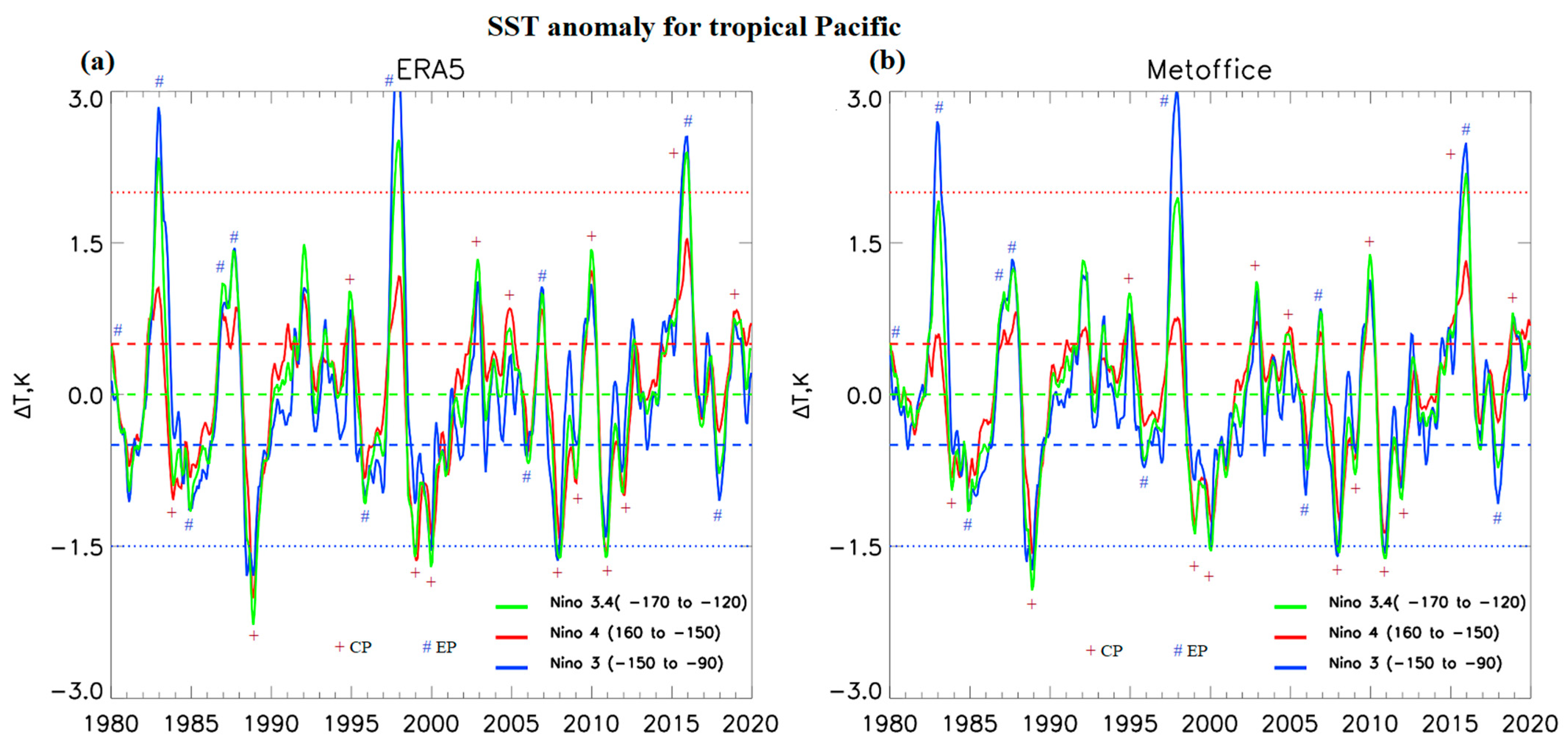
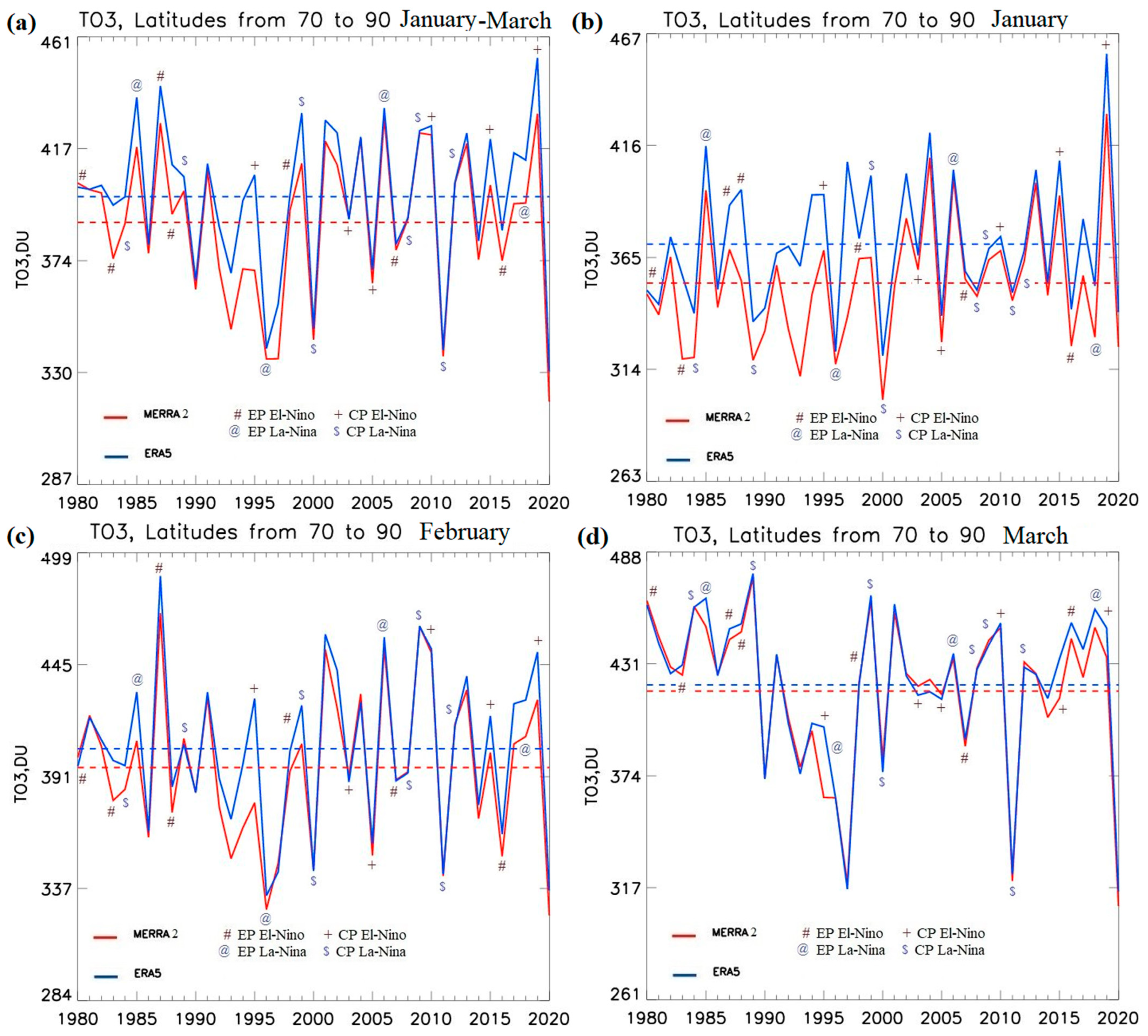
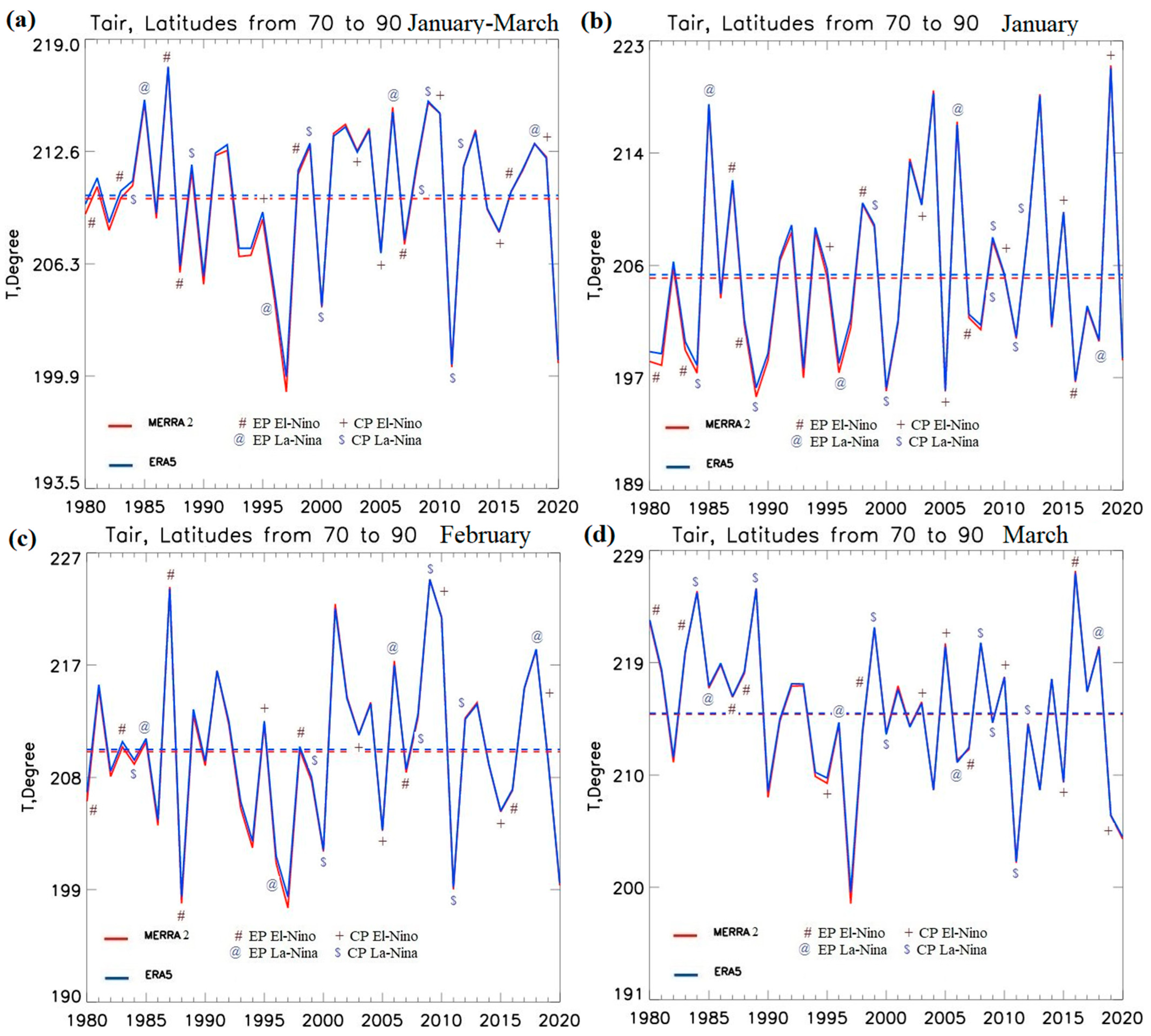
3.1. Analysis of Interannual Variability of Sea Surface Temperature in the Tropical Pacific and Total Column Ozone and Air Temperature in the Arctic Stratosphere

Although previous studies have repeatedly classified ENSO into phases and types (for example [19,74,75,76,77]), this work once again classifies them based on reanalysis data. To increase the validity of the conclusion, two sets of reanalysis data were used: MetOffice and ERA-5. The SST anomalies in the tropical part of the Pacific Ocean in the region of 5 S–5 N, 170 W–120 W (Nino 3.4 area), as well as at 160 E–150 W (Central Pacific) and 150 W–90 W (Eastern Pacific) for the period from 1980 to 2020 are presented in Figure 1. Pronounced El Niño phases, according to the reanalysis data, were observed in 1983, 1987, 1988, 1992, 1995, 1998, 2003, 2005, 2007, 2010, 2016 and 2019, while La Niña phases were observed in 1984, 1985, 1989, 1996, 1999, 2000, 2006, 2008, 2009, 2011, 2012 and 2018. At the same time, the most powerful El Niño events occurred in 1982–1983, 1997–1998 and 2015–2016, when SST anomalies exceeded 2.5 K. The most powerful phases of La Niña were observed in 1988–1989, 1999–2000, 2007–2008 and 2010–2011, when SST anomalies reached −1.5 K. It can also be noted that the pronounced SST anomalies for both El Niño and La Niña cases were reached during the period from December to February, i.e., during the winter months of the Northern Hemisphere. And, consequently, the El Niño and La Niña phenomena reach their maximum development in the winter months, so during these months, the heat and mass flows into the upper tropical troposphere and stratosphere change most strongly compared to the neutral phase.
Based on the analysis of SST anomalies and following previous studies, El Niño and La Niña phases were classified into EP and CP types, respectively. The EP type includes such El Niño and La Niña events when SST anomalies at the 150 W–90 W region (blue line in Figure 1) were above (in the case of El Niño) and below (in the case of La Niña) the SST anomalies at the 160 E–150 W region (red line in Figure 1). Figure 1 demonstrates that the years 1983, 1987, 1988, 1998, 2007 and 2016 can be classified as EP El Niño, while the years 1985, 1996, 2006 and 2018 as EP La Niña. The CP type includes those El Niño and La Niña events at which SST anomalies at 160 E–150 W and 150 W–90 W are close to each other. From Figure 1, it is clear that El Niño 1995, 2003, 2005, 2010 and 2019, as well as La Niña 1984, 1989, 1999, 2000, 2008, 2009, 2011 and 2012, can be classified as CP type. A special case, as previously noted in [18], is the 1992 El Niño, which does not belong to any type—that is, it is an El Niño that changes from the CP type to the EP type. Figure 1 depicts that, for this year, the SST anomalies are largest at 170 W–120 W (green line).
Next, to assess the degree of ENSO phases’ and types’ impact on the processes in the Arctic stratosphere, the monthly mean MERRA2 and ERA5 total column ozone and temperature of the lower stratosphere (15–30 km) in the Arctic region (70–90 N) for the period from 1980 to 2020 were tested for consistency to ENSO phases and types. Interannual variability of Arctic total column ozone averaged over the period from January to March, as well as separately for January, February and March, is presented in Figure 2. Theoretically, during the El Niño phase, the total column ozone content in the Arctic should increase, since with an SST increase in the tropical zone, there is a mass and heat uplift there, followed by meridional transport enhancement from the tropics to the polar stratosphere, while during the La Niña phase, the total column ozone content should decrease due to the weakening of this transport [78,79]. Figure 2, together with the summary data on the anomaly of total column ozone shown in Table 1, demonstrates that out of 22 cases of total column ozone above the average value (dashed lines in Figure 2), according to both reanalysis data, 7 cases correspond to the El Niño phase, 8 cases correspond to the La Niña phase and 7 cases correspond to the neutral phase. Of the 15 cases where, according to both reanalysis data sets, the total column ozone is below average, 5 correspond to the El Niño phase, 3 correspond to the La Niño phase and 7 correspond to the neutral phase. In 1984, 1995, 2003 and 2008, different reanalyses depict anomalies from the average values in opposite directions, but these anomalies are small in magnitude. Overall, these results indicate that it is difficult to definitively say from this analysis that any phase of ENSO is more likely to contribute to a decrease or increase in Arctic ozone.
If we consider significant anomalies from the average value of total column ozone (more than 25 DU), then for such 8 cases of enhanced values, 3 belong to the El Niño phase, 4 belong to the La Niña phase and one case belongs to the neutral phase. For 7 low values, none belong to El Niño, 3 cases belong to La Niña and 4 belong to the neutral phase. At the same time, for the neutral phase with low values in 1990 and 1997, SST anomalies are close to the boundary of the La Niña phase. Thus, from a formal analysis of total column ozone anomalies for the entire winter–spring period from January to March, one can definitely conclude that a significant decrease in Arctic column ozone exceeding 25 DU is more likely for the La Niña phase or the near-La Niña neutral phase.
If we consider the types of ENSO phases, it can be noted that a decrease in the total ozone column to the lowest values is most likely during the CP La Niña (January–March). In 2000 and 2011, total column ozone decreased to 320–365 DU, which is 15–65 DU below the long-term average total ozone. But at the same time, in 1984, 1999 and 2009, the total ozone column was 2–40 units above average, indicating an increase in ozone due to previous strong El Niño (La Niña of 1984 and 1999 followed by strong El Niño of 1983 and 1998) as well as non-ENSO factors. On the EP La Niña, in most cases (1985, 2006 and 2018), the total ozone column reaches from 400 to 460 DU (12–48 DU above average). Although, in 1996, despite the EP La Niña, the total ozone content was 50 DU less than the average. As shown earlier, the La Niña maximum occurs in December–January.
If we consider the January anomalies of the total ozone column (Figure 2), which are determined mainly by dynamic processes [10,20,42], then out of 13 cases of significant ozone reduction, 5 correspond to CP La-Nina, 2—EP La-Nina, 2—EP El-Nino, 1 case—CP El-Nino and 3 cases correspond to the neutral phase. Moreover, in January, of all 8 cases of CP La Niña, only 2 (in 1999 and 2009) occur in winters with high ozone content, and 6 correspond to cases of low total column ozone. SSWs often occur in February and disrupt the stability of the polar vortex, leaving only three significant ozone decreases for La Niña CPs (1984, 2000 and 2011) in this month. In February, the total ozone content in 1989 and 2012 becomes 10–20 DU above average, and in 1999 the anomaly decreases—the total ozone column is above the norm by 20 DU. At the same time, in 1999, there are significant discrepancies between the reanalysis data. In other cases, the anomalies change little. In March, the polar vortex, most often, already begins to collapse as a result of the final warming, and at the same time, after the return of the sun, the chemical destruction of ozone is activated. As a result, the role of dynamic factors is further reduced, and only two episodes of significant ozone decrease remain for the La Niña CP (2000 and 2011).
For the EP La Niña, in February and March, the total ozone column in all cases except 1996 is above the average by 20–60 DU, then, as in 1996, by 10–50 DU below the average. In January, the total ozone column is below the average not only in 1996 but also in 2018. This means that the main impact of EP La Niña appears in February–March (i.e., with a shift of 2–3 months after the event). The impact of CP La Niña has been controversial, since the residual heat of a powerful El Niño (1983–1984 and 1998–1999), as well as processes not associated with ENSO, can impact stratospheric processes, although in most cases CP La Niña contributes to a decrease in total ozone column.
As for the El Niño phase, during the CP El Niño (2003, 2010, 2015 and 2019), the level of the total column ozone in January–March reaches values from 390 to 460 DU (4–50 units above average). At the same time, the data of the 1995 reanalysis gave contradictory estimates: the ERA5 data give a total content of 415 DU (30 DU above average), and the MERRA2 data give 370 DU (16 DU below average). Significant discrepancies in the reanalysis data are observed in 2015 and 2019, but in this case, the total values of the ozone column are higher than the average for all data. At the same time, in 2005 (CP El Niño), the ozone content was 24 DU below the average value. During the EP El Niño, the situation with the total ozone column is ambiguous: in 1980, 1987 and 1998, the total ozone column was 5–45 DU above average, and in 1983 and 2007 it was by 8–14 DU below the average. In 2016, there is a discrepancy in the reanalysis data. At the same time, it can be seen that the main impact of EP El Niño manifests itself in February–March. In January, in all cases except 1987 and 1988, the total ozone column is either below average or close to it, and in February and 1988, the total ozone column anomalies became below average. Only in 1987 did ozone anomalies exceed the average values by 60 DU. At the same time, in all cases, except for 2007 and 2016, there are significant discrepancies in the total ozone column between the reanalyses. The influence of CP El Niño starts to show up already in January and February, as can be seen from 2003, 2010 and 2019, when the total ozone column becomes higher than average by 20–60 DU. In 2005, the total ozone column was 10–30 DU below the average. In 1995, there is a significant discrepancy in the reanalysis data. Thus, El Niño contributes to an increase in ozone in February–March (that is, 2–3 months after the maximum of the El Niño phenomenon).
In the neutral phase, the total ozone column is both above and below average, but it is worth highlighting the years in which the total ozone column decreased to the state of the ozone hole: 1997 and 2020 (in these years, a stable PV was observed). At the same time, in 2020, the ozone content decreased by 78 DU, which is associated with the strongest and most stable for a long time (until April) PV. In addition, in 1997, the ozone content in February became below average, and in January it was above average. Possibly, the strong PV in 1997 and 2020 is associated with processes not related to the ENSO.
In addition to analyzing changes in the total column ozone, changes in air temperature in the Arctic stratosphere were analyzed (Figure 3). The correlation coefficient between air temperature and total ozone content is 0.90–0.95. The figure demonstrates that during the CP La Niña, the air temperature is lower than the long-term average in 2000 by 6.2, in 2011 by 9.6, and in 1999 and 2009 above average by 3.0–5.4 degrees. In 1989, 2008 and 2012, air temperatures were slightly higher than the long-term average. During CP La Niña, the probability of an SSW is minimal, although an SSW is still possible due to non-ENSO factors as well as residual heat from strong El Niño events (1984 and 1999). During the EP La Niña (1985, 2006 and 2018), the temperature exceeds the long-term average by 3.0–5.4, although in 1996 it is below the average by 5.8. During the CP El Niño (2003, 2010 and 2019), the temperature in the Arctic stratosphere is 2.7–4.8 above the long-term average, although in 1995 and 2005, it was 1.2–3.0 below average. During the EP El Niño, air temperatures in 1983, 1987, 1998 and 2016 were 0.4–7.4 above average (in 1998, during a powerful El Niño, it was 1.4 above normal and in 1987—7.4 above the norm), although in 1988 and 2007, the temperature was 2.6–4.2 below average. In the neutral phase, the air temperature in the Arctic stratosphere is both below and above average, but it is worth highlighting, as in the case of the total ozone column, 1997 and 2020, when the air temperature was below the long-term average by 9.3–11.0 degrees, which is associated with stable PV in these years due to processes not related to ENSO.
Thus, it turns out that both types of phases of El Niño and EP La Niña contribute to the formation of SSW and an increase in ozone content in the Arctic stratosphere, and CP La Niña will lead to a decrease in air temperature and a decrease in ozone content (although in some cases with La Niña CPs, SSWs and increased ozone levels are also observed). This is due to the fact that during the CP and EP phases of El Niño and EP La Niña, the transfer of heat and mass from the troposphere to the stratosphere and from the equator to the pole increases, which leads to an increase in air temperature in the stratosphere. An increase in heat and mass transfer contributes to an increase in the residual meridional circulation and the flow of wave activity, which affects the zonal wind and destroys the PV. As a result, the Brewer–Dobson circulation intensifies, which leads to an increase in the total ozone column.
According to previous studies [19,42,75,77], during the El Niño phase, in most cases, the PV weakens and becomes unstable. During the La Niña phase, the heat flux into the stratosphere decreases, which contributes to the stability of the PV, as a result of which the PV can exist until March–April. However, there are exceptions—in 1998–1999, the PV was very unstable, despite La Niña (perhaps this is due to the residual heat from El Niño 1997–1998, as well as other processes in the atmosphere) [19]. This means that the El Niño phenomenon contributes to PV instability, but does not necessarily lead to it, since PV is also affected by other processes such as solar activity, the Quasi-Biennial Oscillation and the North Atlantic Oscillation [42]. The same applies to the La Niña phase. The analysis carried out in this article showed that not only the ENSO phase, but also its type, play a key role in the total ozone column and air temperature in the stratosphere, and, hence, on the PV, which confirms the conclusions in [42]. During the CP La Niña, heat and mass transfer to the Arctic stratosphere is attenuated, which contributes to sustained PV and ozone depletion, although there are exceptions (1999 and 2009).
It can also be seen that the impact of El Niño and La Niña manifests itself in February–March, that is, with a shift of 2–3 months after the maximum of the event. If in January the air temperature during El Niño can be both above and below the average (as can be seen from Figure 3), then, in February, the SSW associated with El Niño begins to manifest itself—the air temperature becomes 2–20 above the average (before except for 1988 and 2005 when it was 5–10 below average). In March, the air temperature during El Niño is either close to or above average. At the same time, during the CP El Niño, the SSW occurs earlier (i.e., in January–February) than during the EP El Niño, as can be seen from the graphs. As for La Niña, its type plays the greatest role. In the CP La Niña, the air temperature is either close to or below average (in 2000 and 2011—5–10 below average), except for 1999 and 2009 (in March—2008), when the air temperature was 5–10 above average. During the EP La Niña, in all cases except 1996, the air temperature was 5–15 degrees higher than the average, which indicates powerful SSWs. Only in 1996 was it below average. But even in the neutral phase, there may be years with a stable PV and an ozone hole (1997 and 2020). At the same time, in 1997, the air temperature in January was above average. It is possible that the steady decrease in PV and temperature in 1997 and 2020 is associated with processes not related to the ENSO.
Based on this analysis, as well as review [18,42], a table of ENSO phases was constructed by their types and values of SST anomalies, as well as anomalies of the total ozone column and air temperature in the stratosphere at 70–90 N, presented below in Table 1. The table of SST anomalies shows that in 1980, 1983, 1987, 1988, 1998, 2007 and 2016, EP El Niño was observed (marked in red in the table). CP El Niño was observed in 1995, 2003, 2005, 2010, 2015 and 2019 (marked in yellow in the table). EP La Niña events were observed in 1985, 1996, 2006 and 2018 (marked in green in the table). CP La Niña events were observed in 1984, 1989, 1999, 2000, 2008, 2009, 2011 and 2012 (marked in blue in the table). El Niño 1992 and La Niña 2001 were also observed, which do not belong to any type (marked in gray). The most powerful were EP El Niño of the 1983, 1998 and 2016 types (SST anomalies over 2 degrees), and CP La Niña of the 1989, 2000 and 2011 types (SST anomalies over −1.1 degrees). The duration of the event also matters. The longer the duration of the ENSO event, the stronger its impact. The longest were EP El Niño 1982–1983 (16 months), EP El Niño 1986–1988 (17 months), CP La Niña 1988–1989 (16 months), CP La Niña 1998–2000 (25 months), CP La Niña 2010–2012 (21 months), El Niño 2014–2016 (19 months, which started as CP but became EP) and CP El Niño 2018–2019 (16 months). At the same time, it is also worth paying attention to some years with a neutral phase: 1986 (for 3 months in Nino3, the SST anomaly was less than −0.5), 1997 and 2013 (for 4 months in Nino4, the SST anomaly was less than −0.5), 2002 (during 5 months in Nino4, the SST anomaly was less than −0.5) and 2020 (in Nino3, the SST anomaly was more than 0.5 after El Niño 2018–2019). The year 1980 is disputable—the SST reanalysis data give a neutral phase (exceeding 0.5 degrees for no more than 3 months), but other studies give EP El Niño [18], so in the table, 1980 is still marked as EP El Niño.
As for the total ozone column, the anomaly values below −25 DU are marked in blue in the table, while those above 25 DU are marked in pink. The table shows that the decrease in the total ozone column to the state of the ozone hole (anomalies less than −25 DU) was in 1990, 1993, 1997 and 2020 (neutral phase), 2000 and 2011 (CP La Niña), 1996 (EP La Niña) and 2005 (CP El Niño, according to ERA5). Increases in ozone (anomalies over 25 DU) were in 2004 (according to MERRA2) and 2013 (neutral phase), 1987 (EP El Niño), 2010 and 2019 (CP El Niño), 1985 and 2006 (EP La Niña), 1999 (ERA5) and 2009 (CP La Niña) and 2001 (La Niña). Air temperature anomalies in the Arctic stratosphere, in general, correspond to the ozone content: with anomalies of the total ozone column of less than −25 DU, the temperature anomalies are less than −3.3 degrees, while with anomalies of more than 25 DU, the temperature anomalies are more than 3 degrees (except for 2019, where temperature anomalies are in the region of 2.1–2.4 degrees).
Thus, the decrease in the total ozone column and the formation of ozone holes are associated with a decrease in temperature in the Arctic stratosphere, which is a consequence of a stable PV. An increase in the total ozone column is associated with the warming of the Arctic stratosphere and SSW, which lead to the destruction of the PV and an increase in the Brewer–Dobson circulation, which increases the total ozone column. A decrease in air temperature in the Arctic stratosphere and a decrease in the total ozone column are most likely in years with a neutral phase and CP La Niña, while an increase in temperature, SSW, and an increase in ozone occur in years with EP La Niña and CP El Niño. However, in general, no direct significant relationship between ENSO and SSW and total ozone column was found when considering the entire time period from 1980 to 2020, since not all El Niño and La Niña phases observed during this period are strong enough to have a significant impact on the stratosphere; moreover, the Arctic stratosphere is also affected by processes not associated with ENSO [18].
Anomalies of the total ozone column and air temperature in the Arctic stratosphere for January, February and March were also analyzed separately. The data are presented in Table 2. As shown earlier, the influence of ENSO is manifested in the Arctic stratosphere in February–March, while in January, the ozone content and air temperature are influenced by factors not related to ENSO.
A decrease in the total column ozone to extremely low values (anomaly less than −25 DU) was often observed in years with a neutral ENSO phase: in January these were 1981, 1990, 1993 and 2020, in February—1986, 1993, 1994. Of these, we can highlight the years 1990, 1993 and 2020, when the overall ozone column anomaly was consistently below −25 DU throughout the winter period, indicating stable PV in these years. In January 1997, the total ozone column was high (an anomaly of more than 25 units), but in February, it changed to more than −25 units, which is associated with a stable PV. In terms of ENSO phases, total ozone was lowest in 1996, 2000 and 2011 (CP La Niña), and 2005 (CP El Niño) from January to March (in 2011 from February to March). That is, the decrease in the total ozone column to extremely low values during the La Niña CP is more frequent than during other ENSO phases and types. Therefore, during the CP La Niña, the PV is more stable and the SSW is less likely than during other ENSO phases. It should be noted that the La Niña CPs of 2000 and 2011 are the longest, lasting more than 20 months, which can also affect the stability of the PV and the total column ozone, leading to the formation of extremely low values.
As for the increase in the total ozone column to high values (an anomaly of more than 25 DU), in this case, the relationship with ENSO appears to be more significant. In January, the teleconnection with the ENSO is insignificant—the excess of the ozone anomaly by more than 25 DU was noted in the years with the neutral phase—1997, 2002, 2004 and 2013, as well as in 1988 (EP El Niño), 2015 and 2019 (CP El Niño), 1985 and 2006 (EP La Niña) and 1999 (CP La Niña). In February, the situation began to change—the total ozone column increased in 1981 and 1991 (neutral phase) but decreased in 1997 to the state of the ozone hole. Possibly, the situation in 1997 (the ozone anomaly is higher by 25 DU in January) is related to the residual influence of the 1996 EP La Niña, although there may be factors not related to the ENSO. At EP El Niño, the total ozone column increased in 1987, at CP El Niño, in 2010, and at CP La Niña, in 2009 (while decreasing in 1999). In March, the impact of ENSO is quite significant: the total ozone column increased: during the EP El Niño in 1980, 1987, 1988, and 2016; during the CP El Niño in 2010 and 2019; during the EP La Niña in 1985 and 2018; during the CP La Niña in 1984, 1999, and 2009, and only in 1981 during the neutral phase. It should be noted that El Niño 1987–1988 and 2016 are quite long—more than 15 months, which also leads to an increase in the SSW and an increase in the total ozone column.
Thus, it turns out that an increase in the total ozone column to high values (an anomaly above 25 DU), and, consequently, an SSW, is most likely during the El Niño phase and the EP La Niña (as can be seen from the total ozone column anomalies in March) (Table 3). A decrease in the total ozone column to the state of an ozone hole (an anomaly less than −25 DU), and, consequently, a stable PV and a decrease in temperature in the Arctic stratosphere, are most likely during the neutral phase (Table 3). The impact of the CP La Niña phase is ambiguous—it gives both a decrease in the total ozone column to the state of the ozone hole (2000 and 2011) and an increase in the total ozone column (1999, 2009), which may be associated with the duration of La Niña—more than 20 months in 2000 and 2011, and less than a year otherwise. Based on the analysis of graphs and tables, a final table of the number of years was constructed depending on the anomalies of the total ozone column and ENSO phases for the period from January to March, as well as for each of these months.
In addition to ENSO, the stability of the PV, and hence the total ozone content, is influenced by DWC, as well as ozone waves and QBO. As studies [59,60,61] show, a stable PV and a decrease in total ozone content to the ozone hole state are observed in years with strong DWC, while in years with weak DWC, the PV becomes unstable, and the total ozone content increases. The analysis of ENSO phases and total ozone content shows that strong DWC probably occurs during the neutral phase and CP La Niña, while El Niño and EP La Niña phases contribute to the weakening of DWC due to increased heat and mass fluxes and wave activity into the polar stratosphere. Meanwhile, the total ozone and PV content in the polar stratosphere are also affected by radiation-related ozone waves [62] and the QBO phase [63]. The intensification of ozone waves leads to an increase in total ozone content during the fall months and early winter [62]. As for the QBO phase, in this case, the western phase contributes to a stronger PV and lower total ozone content, whereas the eastern phase contributes to a weaker PV and higher total ozone content [63]. Differences related to the ENSO influence (especially the CP La Niña phase) can be related to different QBO phases, as well as to different phases of solar activity, which has an influence on ozone waves.
Based on the analysis of SST anomalies, the total ozone column, and air temperature, the years with the most characteristic SST values for the ENSO phase and its type, and the impact on dynamic and chemical processes in the Arctic stratosphere, were selected. For EP El Niño, these are 1982–1983, 1997–1998 and 2015–2016; for CP El Niño, 2002–2003, 2009–2010 and 2018–2019; for EP La-Nina, 1984–1985, 2005–2006 and 2017–2018, for CP La Niña, 1988–1989, 1999–2000 and 2010–2011. Over the years, the average values for the zonal wind, ozone concentration, and air temperature were calculated, which makes it possible to analyze the processes in the Arctic stratosphere associated with the state of the PV, which is presented later in the article.

3.2. Analysis of Telecommunications and ENSO Impacts on the Stratosphere and Ozone Layer

For a detailed analysis of the processes of interaction between the troposphere and stratosphere in different phases of El Niño and La Niña, average values were calculated for years with EP and CP El Niño and EP and CP La Niña. For the analysis of stratospheric dynamics, only MERRA-2 data are used further, since ERA-5 data are available at pressure levels only up to 1 mb (about 48 km), while atmospheric dynamics was considered up to heights of about 60 km, since the residual circulation and wave activity in the upper stratosphere and lower mesosphere also affect processes in the middle and lower stratosphere. Figure 4 shows the zonal average profiles of zonal wind speed at 64 N latitude. Differences in El Niño and La Niña ozone concentrations for EP and CP types, as well as differences between EP and CP types for El Niño and La Niña (ozone concentration anomaly) at 80–90 N, are shown in Figure 5. Figure 6 and Figure 7 show the average zonal air temperature profiles at 70–90 N latitude, and ozone concentration at 80–90 N latitude.
To explain the reasons for changes in the concentration and total column ozone depending on ENSO, dynamic and thermal processes in the stratosphere were studied. To carry this out, the zonal wind speed at the boundary of the polar region and the air temperature inside it was analyzed. Figure 4 demonstrates that in the El Niño phase, the zonal wind reaches 20 m/s from November to January on the El Niño VP and until December on the El Niño CP, after which it decreases to values less than 10 m/s and changes sign in the opposite direction, which is a sign of the destruction of the PV. During the CP La Niña phase, the zonal wind in the winter months has large positive values (more than 30 m/s), which indicates a stable PV and westerly transport of air mass. Only in April does the zonal wind change to the opposite direction. However, during the La Niña EP, the zonal wind from January weakens to values less than 10 m/s and changes sign, which indicates the destruction of the EP. The correlation coefficients between zonal wind and ENSO phases are 0.75–0.85.
An area of positive zonal wind values with values greater than 15 m/s over the Arctic is a sign of the presence of a stable PV, so its decrease below this threshold indicates instability of the PV. Of particular importance are the values of the zonal wind at the boundary of the polar region (about 64 N), which can be considered a characteristic of the degree of isolation of polar latitudes from the exchange of heat and mass with mid-latitudes. If the values of the zonal wind over the Arctic, and especially 64 N, change sharply, then the PV becomes unstable. Zonal wind patterns can be influenced by atmospheric processes, most notably the Quasi-Biennial Oscillation, North Atlantic Oscillation and ENSO. The impact of ENSO is due to the transfer of heat and mass from the troposphere to the stratosphere [20,80,81]. During El Niño, the lower troposphere warms, causing the Aleutian Low to deepen. As a result, the vertical transfer of heat and mass into the upper troposphere, as well as into the lower stratosphere, increases. This leads to an increase in temperature in the stratosphere and SSW. Since warm air is less dense than cold air, the values of pressure and geopotential change, and, consequently, the values of pressure gradients. An increase in temperature in the stratosphere and in the SSE leads to a decrease in the temperature contrast between the Arctic and tropical stratosphere, which leads to a decrease in pressure gradients. A decrease in pressure gradients leads to a weakening of zonal transport in the stratosphere and, as a consequence, to a weakening of PV. Therefore, during strong El Niño years, the zonal wind over the Arctic weakens, leading to PV instability. In addition, the type of El Niño is also important: with a CP El Niño, the PV is destroyed in January, and with an EP El Niño—in February. Therefore, during an EP El Niño, the PV is more stable than during an EP El Niño. In years with the CP La Niña phase, the transfer of heat and mass into the stratosphere weakens, the Aleutian Low fills, which contributes to a decrease in temperature in the stratosphere, so the temperature contrast between the Arctic and tropical stratosphere increases. As a result, pressure gradients increase and, as a consequence, the zonal wind intensifies, which leads to a weakening of the SSW and a stable PV. However, during the EP La Niña, the zonal wind weakens and changes sign, leading to PV instability, indicating an increase in heat and mass fluxes in the atmosphere and the EP. Thus, it turns out that the CP La Niña contributes to a weakening of heat and mass fluxes into the atmosphere, while the CP La Niña contributes to its increase. This may be due to an increase in temperature and pressure contrast between the western and eastern areas of the Pacific Ocean during the La Niña EP. It is also known that, in 1999, there was an increase in temperature in the stratosphere and a powerful SSW, as a result of which the PV turned out to be unstable, despite the fact that in 1999, the CP La Niña phase was observed. This may be due to residual heat from the powerful El Niño of 1998, as well as the influence of non-ENSO processes [82].
To assess the impact of changes in PV on the ozone layer due to changes in ENSO phases and types, the relative percent differences in ozone concentrations between the two ENSO phases and between the two types for each ENSO phase were calculated (Figure 5). As can be seen from the figure, in the case of the EP type, the ozone concentration during La Niña exceeds the concentration during El Niño by 20% in January and by 20–40% in February, and in other months, the anomalies are insignificant. But in the case of the CP type, the ozone concentration during El Niño is higher than the La Niña concentration from January to March by 30–40%, while in September–October, it is lower by 20%, and in April, it is lower by 30% than in La Niña. During the El Niño phase, it is seen that with the EP type, the ozone concentration is lower than with the CP type by 20–30% in January–February, and in March–April, it is 10–20% higher. During the La Niña phase, the ozone concentration in the EP type is higher than in the CP type by 20–40% from December to March and lower by 10–20% in September–October and April.
It is also clear that the difference in ozone concentration anomalies between the El Niño types, as well as between the El Niño and La Niña WP types, is generally insignificant: only negative anomalies are noticeable (by 20–40% in January–February) in certain periods of time (approximately 10–20 days) and not at all altitudes. However, if we compare the La Niña CP type with the La Niña CP or El Niño CP, then a significant anomaly is observed in the winter months, amounting to 20–40% in the winter months throughout the entire thickness of the atmosphere. This means that the La Niña CP contributes to a significant decrease in ozone concentrations in the Arctic stratosphere during the winter months, which is associated with a stable PV and the absence of SSW. In other cases, SSWs occur in the stratosphere, which leads to a weakening of the PV and an increase in ozone concentration. At the same time, in the case of EP El Niño, the SSW occurs later (in February) than during EP El Niño and EP La Niña, therefore, the ozone concentration during EP El Niño is lower than during EP El Niño and EP La Niña, but higher than CP La Niña.
An analysis of the variability of ozone concentration demonstrates (Figure 6) that at low temperatures and stable PV in the Arctic stratosphere, extremely low ozone concentrations of less than 4.0 ppm or 6.7 × 10⁻⁶ kg/kg were registered. Analysis of zonal wind and air temperature found that only CP La Niña conditions contribute to a decrease in air temperature in the stratosphere, which reduces the probability of SSWs by weakening vertical heat fluxes into the stratosphere and leads to the depletion of stratospheric ozone. During the El Niño phase, conditions are formed that contribute to an increase in air temperature in the stratosphere and an increase in the probability of SSW, which leads to instability of PV and an increase in ozone concentration in the Arctic stratosphere. However, low ozone concentrations can also be observed during the El Niño phase, but with the EP type. This is due to the fact that the decrease in ozone concentration occurs due to the fact that, during the EP El Niño period, the PV is destroyed later (in February) than during the CP El Niño (in January). In addition, the decrease in ozone concentration occurs not only due to heat flows from the troposphere to the stratosphere and dynamical processes, but also as a result of photochemical processes initiated by heterogeneous processes on polar stratospheric clouds involving chlorine and bromine. During the EP La Niña, strong SSWs and weakening PVs occur more often, as shown by analysis of zonal wind speed and temperature, and, therefore, the EP La Niña contributes to an increase in ozone concentrations in the stratosphere of the Northern Hemisphere. Figure 6 also depicts that during the EP-type El Niño and La Niña in the autumn months, the ozone concentration is lower than during the CP-type, which may be due to the intensification of the chemical processes of ozone destruction on polar stratospheric clouds in the autumn months. The correlation coefficients of ozone concentration with zonal wind (Figure 4) are 0.85–0.90 and with ENSO phases are 0.7–0.8. The correlation coefficients of ozone concentration anomalies (Figure 5) with ENSO phases are 0.75–0.90.
An analysis of air temperature variability, which characterizes the degree of stability of air pollution and ozone depletion, is presented in Figure 7. As can be seen from the figure, during the El Niño phase, powerful SSWs are observed in February–March in the case of EP El Niño and in January–February in the case of CP El Niño. After the SSW, the region of low temperatures in the Arctic stratosphere quickly disappears, and if it is restored, it is in a weak and unstable form. During the CP La Niña, SSWs are rare and weaker than during El Niño, which leads to a fairly stable region of low temperatures in the Arctic stratosphere, a stable PV and a decrease in ozone concentration. However, during the EP La Niña in January–February, powerful SSWs are registered, which, as in the case of El Niño, lead to warming in the Arctic stratosphere. The correlation coefficients of air temperature with ozone concentration (Figure 6) are 0.8–0.9, with zonal wind—0.7–0.8, with ENSO phases—0.7–0.8.
In years with strong SSWs, the PV destabilizes and weakens, and in years without SSWs, it exists stably. It follows that El Niño and La Niña CP, which contribute to strong SSWs, also contribute to the destabilization of the PV, and the La Niña CP contributes to the weakening of the SSW and the stabilization of the PV. Thus, El Niño and EP La Niña contribute to an increase in ozone content, and CP La Niña—to a decrease. Similar results were obtained from the ERA 5 reanalysis data for air temperature, zonal wind speed and ozone concentration.
The lowest values of air temperature are typical for years with stable PV, whereas high values of temperature correspond to a weakened or unstable PV, especially if SSW occurs in January–February. This is due to the fact that after the formation of PV, the stratosphere cools, resulting in the formation of a low-temperature region, and a temperature gradient appears that maintains PV. If the PV is weakened or unstable, then the region cools slightly. If the temperatures in the Arctic stratosphere are sufficiently high (more than 200 K), then there is no temperature gradient, as a result of which the PV is formed only due to dynamical factors and will be less stable. In this case, periods of low temperatures, as is well known, can be interrupted by SSW, which can impact the stability of the PV. As mentioned earlier, the increase in temperature in the stratosphere and SSW can be caused by El Niño, which lead to the deepening of the Aleutian minimum and the vertical flux of heat into the stratosphere [20,80,81].
At the same time, the type of El Niño also influences SSW formation: during the CP El Niño, the SSW is observed in January, and during EP El Niño, in February. Therefore, during EP El Niño, the PV is more stable than during CP El Niño. However, SSWs can also be observed during EP La Niña [20,80,81], which may be associated with an increase in the heat flux into the stratosphere due to the contrast between the eastern and western parts of the Pacific Ocean. The more intense and longer the SSW, the less stable the PV. It can also be seen that the impact of ENSO on stratospheric processes does not appear immediately, but with a delay of approximately 1–3 months, which is associated with the inertia of atmospheric processes (for example, the deepening of the Aleutian Low) and the need for heat flux to overcome different layers of the atmosphere, including inversion layers.
As is known, the Brewer–Dobson circulation has a significant impact on the ozone content. During the El Niño phase, the heat flux into the atmosphere increases, which leads to a positive PNA phase and an increase in the eastward jet stream towards North America [42]. As a result, pressure increases in the area of the Hawaiian Islands and decreases over the Aleutian Islands (deepening of the Aleutian Basin). This leads to an increase in the meridional heat and mass transfer, which leads to an increase in the meridional residual circulation, which impacts the zonal wind and leads to PV instability. As a result, the PV weakens, which leads to an increase in the exchange of air masses between the equatorial and polar latitudes. This process enhances the Brewer–Dobson circulation, which transports ozone produced in the tropical stratosphere as a result of photochemical processes to the polar latitudes. Thus, El Niño contributes to an increase in the concentration and total content of ozone in the Arctic stratosphere. At the same time, the intensification of the residual meridional circulation and the Brewer–Dobson circulation occurs both during the EP El-Nino and during the CP El Niño, which means that both types of El Niño contribute to an increase in the ozone concentration in the Arctic stratosphere. At the same time, during EP El Niño, the impact on the zonal wind is weaker than during CP El Niño, since the SSW during EP El Niño occurs later than during CP El Niño, so the ozone content due to increased BD circulation will increase faster during CP El Niño than during EP El Niño.
During the CP La Niña phase, the transfer of heat and mass from the troposphere to the stratosphere weakens, which leads to an increase in pressure over the Aleutian Islands (filling of the Aleutian depression) and a decrease in pressure over the Hawaiian Islands, and a negative PNA phase (the jet stream is directed to the west, in side of Asia). As a result of all this, the temperature contrast between the Arctic and the tropics increases in the stratosphere, which leads to an increase in the zonal wind and PV stability. In this case, the meridional transfer between high and low latitudes is weakened. As a result, the meridional transfer of air masses from the equator to the pole in winter is insignificant, while the PV and zonal transfer are stable. Thus, the CP La Niña phase contributes to the weakening of the BD circulation, as a result of which the concentration and total content of ozone in the Arctic stratosphere decrease to the state of an ozone hole. However, during the EP La Niña phase, on the contrary, there is an increase in the BD circulation. It is possible that the increase in temperature contrast between the western and eastern parts of the Pacific Ocean during the EP La Niña leads to a deepening of the Aleutian Low, which contributes to an increase in the heat flux into the stratosphere and SSW. As a result, during the EP La Niña, the zonal wind and PV weaken, while the residual meridional circulation increases, which leads to an increase in the BD circulation and an increase in the concentration of ozone in the Arctic stratosphere.

3.3. Analysis of Residual Circulation, Brewer–Dobson Circulation and of Wave Activity Fluxes of Stratosphere

As is known, the Brewer–Dobson circulation has a significant impact on the ozone content. To assess the impact of ENSO on the Brewer–Dobson circulation and on the distribution of ozone in the atmosphere, a residual circulation analysis was carried out. Figure 8 shows the residual meridional circulation for the El Niño and La Niña phases of two types for January, February and March.
It can be seen from the figures that there are two main residual circulation cells in the atmosphere with ascending fluxes at low and middle latitudes of the Southern Hemisphere and descending fluxes at high latitudes of both hemispheres. In contrast to the mean Euler circulation, the residual circulation consists of two Hadley cells propagating from the equator to the pole [70]. At the same time, in winter, the circulation cell in the Northern Hemisphere is larger than in the Southern Hemisphere, and the velocity of the residual meridional and vertical wind is higher [70]. At altitudes less than 60 km, it can be observed that both components of the residual circulation give two cells: a smaller one in the Southern Hemisphere and a larger one in equatorial latitudes and in the Northern Hemisphere, which is typical for winter [70]. During the El Niño phase of both types over the Arctic from January to March, the values of this component are positive and reach 1–2 m/s. At the same time, at heights of 20–25 km above the Arctic, an increase in meridional transport is observed by 1–2 m/s during EP El Niño and by 0.5–1 m/s during CP El Niño. During the CP La Niña phase, a relatively stable area of negative values of the meridional component of the residual circulation (up to −2 m/s at altitudes of 30–40 km) is observed over the Arctic. However, during the EP La Niña over the Arctic, the values of the meridional component at heights up to 35 km are positive and reach 0.5–1 m/s, which indicates an intensification of the Brewer–Dobson circulation, as in the case of El Niño. The correlation coefficients between the residual circulation and ENSO phases are 0.85–0.95.
During the El Niño phase, the heat flux into the atmosphere increases, which leads to a positive PNA phase, and an increase in the jet stream to the east towards North America [42]. As a result, pressure increases in the area of the Hawaiian Islands and pressure decreases over the Aleutian Islands (deepening of the Aleutian depression). This leads to an increase in the meridional transfer of heat and mass, leading to an increase in the meridional residual circulation, which affects the zonal wind and leads to PV instability. As a result, the PV weakens, which leads to an increase in the exchange of air masses between the equatorial and polar latitudes. This process enhances the Brewer–Dobson circulation, which transports ozone produced in the tropical stratosphere by photochemical processes to the polar latitudes. Thus, El Niño contributes to an increase in the concentration and total content of ozone in the Arctic stratosphere. At the same time, the intensification of the residual meridional circulation and the Brewer–Dobson circulation occurs both during EP and CP El Niño, which means that both types of El Niño contribute to an increase in the ozone concentration in the Arctic stratosphere.
During the CP La Niña phase, the transfer of heat and mass from the troposphere to the stratosphere weakens, which leads to an increase in pressure over the Aleutian Islands (filling of the Aleutian depression), and a decrease in pressure over the Hawaiian Islands, and a negative PNA phase (the jet stream is directed westward, towards Asia). As a result of all this, the temperature contrast between the Arctic and the tropics increases in the stratosphere, which leads to an increase in the zonal wind and to the stability of the PV. In this case, the meridional transfer between high and low latitudes is weakened. As a result, the meridional component of the residual circulation and the meridional transport of air masses from the equator to the pole in winter are insignificant, while the PV and zonal transport are stable. Thus, the CP La Niña phase contributes to the weakening of the Brewer–Dobson circulation, as a result of which the concentration and total column of ozone in the Arctic stratosphere decrease to the state of the ozone hole. However, during the EP La Niña phase, on the contrary, there is an increase in the residual meridional circulation. It is possible that the increase in temperature contrast between the western and eastern parts of the Pacific Ocean during the EP La Niña leads to a deepening of the Aleutian depression, which contributes to an increase in the heat flux into the stratosphere and SSW. As a result, during the EP La Niña, the zonal wind and PV weaken, while the residual meridional circulation increases, which leads to an increase in the Brewer–Dobson circulation and an increase in the concentration of ozone in the Arctic stratosphere.
To analyze the processes associated with wave activity in the atmosphere, the Plumb flux of wave activity was considered. The meridional and vertical components of the wave activity flux and the divergence of the wave activity flux are analyzed. For the analysis, we used the results of calculations for the El Niño and La Niña phases of the EP and CP types. The analysis was carried out for January, February and March, since these months are of great importance for the analysis of PV and the flux of wave activity in the Northern Hemisphere. This is due to the fact that, in winter, the amplitudes of planetary waves reach their maximum values [71], and, as shown earlier in this article, the impact of ENSO on processes in the Arctic stratosphere is maximally manifested precisely in the winter months. During these months, wave propagation increases from west to east, from the equator to the pole and back, and also in the vertical direction [71]. At the same time, the propagation velocity and amplitudes of these waves may depend on the stability of the PV and heat fluxes in the atmosphere associated, in particular, with the ENSO [71]. Fluxes of wave activity can impact zonal wind and PV, as well as the Brewer–Dobson circulation and, consequently, the propagation of ozone in the stratosphere [71].
Figure 9 and Figure 10 show the average vertical zonal profiles of the meridional and vertical components of the wave activity flux for January, February and March.
As can be seen from Figure 9 and Figure 10, in the Northern Hemisphere at altitudes of 20–60 km, large values of the wave activity flux are observed: the meridional component is up to −150 m2 s−2, and the vertical component is up to 0.5–0.8 m2 s−2. This means that, during the winter months in the Northern Hemisphere, there is an increase in the wave activity flux in the stratosphere, which is associated with the presence of heat and mass transfer through the planetary Rossby waves in the Northern Hemisphere during the winter months. The correlation coefficients between the Plumb wave activity flux and ENSO phases are 0.7–0.9. The correlation coefficients between the vertical component of the Plumb flux and SSW events are 0.75–0.90.
During the EP El Niño phase, the meridional component of the wave activity flux in the Arctic stratosphere reaches values from −150 m2 s−2 in January to −100 m2 s−2 in February and up to −50 m2 s−2 in March, while the vertical component changes from 0.8 m2 s−2 in January to 0.8 m2 s−2 in February and up to 0.2–0.3 m2 s−2 in March. That is, in January–February, during the EP El Niño, the wave activity flux is the most powerful. During CP El Niño, the meridional component changes from −80 m2 s−2 in January to −50 m2 s−2 in March, and the vertical component changes from 0.7 m2 s−2 in January to 0.4 m2 s−2 in March. This means that during El Niño, an increase in the transfer of heat and mass from the troposphere to the stratosphere leads to an increase in the wave activity flux from the equator to the pole and from the troposphere to the stratosphere, which leads to an increase in the SSW and a weakening of the zonal wind and PV destruction. As a result of PV destruction, the Brewer–Dobson circulation intensifies, which leads to an increase in the ozone content in the atmosphere of the Northern Hemisphere. At the same time, during EP El Niño, the wave activity flux is stronger than during CP El Niño.
During the CP La Niña phase, the meridional component of the wave activity flux decreases to −20 m2 s−2 in February, and the vertical component to 0.1–0.2 m2 s−2 in February, which indicates a weakening of wave activity in the northern hemisphere. Thus, the phase of CP La Niña contributes to a decrease in the wave activity flux and, consequently, to an increase in zonal transport and an increase in PV. As a result, the probability of SSW decreases, and the Brewer–Dobson circulation weakens, so the concentration of ozone in the northern hemisphere can decrease down to the state of the ozone hole. As for the EP La Niña, in this case, the meridional component of the wave activity flux changes from −150 m2 s−2 in January to −70 m2 s−2 in March, and the vertical component changes from 0.8 m2 s−2 in January up to 0.8 m2 s−2 in February and up to 0.3–0.4 m2 s−2 in March. Thus, it turns out that, in contrast to the CP La Niña, the EP La Niña contributes to an increase in the wave activity flux into the Arctic stratosphere, which can also contribute to the SSW, and hence to the destruction of the PV and the intensification of the Brewer–Dobson circulation, leading to an increase in the total ozone column in the atmosphere of the Northern Hemisphere.
At the same time, it is shown that the EP El Niño leads to the greatest increase in the wave activity flux, which can be seen from the components of this flux and from the wave amplitudes. However, the most powerful SSWs and the greatest destruction of PV are observed precisely during CP El Niño and EP La Niña. This means that heat fluxes into the stratosphere and intensification of the residual meridional circulation still play the greatest role in the destruction of PV. However, the wave activity flux also has a significant impact on the PV and ozone concentration, as seen in the CP La Niña and EP El Niño: it is possible that it was the wave activity flux that led to the SSW and the increase in ozone concentration in the case of the EP El Niño.

4. Discussion

Based on the MERRA2 reanalysis data, the response of the Northern Hemisphere stratosphere to ENSO was studied, which differs depending on the two types of El Niño and La Niña: East Pacific and Central Pacific. In addition, taking into account previous results [42,83], the connection and response of ENSO in the stratosphere of middle and high latitudes for the Northern Hemisphere were analyzed. Our study complements previous studies [18,30,31,35,36,37,42,84,85,86,87,88,89] showing the weakening of stratospheric PV associated with El Niño and the heterogeneity of the Northern Hemisphere PV response to El Niño and La Niña in the cold half-year [90]. We emphasize that both of these features of the response of the polar stratosphere strongly depend on the types of El Niño and La Niña.
It is shown that the weakening of PV in the Arctic is observed in the stratosphere in February in response to the EP El Niño, and during the CP El Niño in November and December, the PV is weaker than during the EP El Niño and sharply weakens in January, although other studies [42] during the CP El Niño show an increase in PV in January. Thus, the response of the stratospheric circulation is the same for the two types of El Niño in February and the opposite in January. These differences may be related to the later SSW in EP El Niño, while the SSW occurs earlier in CP El Niño. According to the MERRA2 data, during the EP El Niño, the SSW occurs in February, although in 1997–1998, the SSW was in January; at the same time, it is considered in [91] that there was no SSW during the EP El Niño at all. At the same time, during EP El Niño, the spring warming of the stratosphere occurs earlier than during La Niña, especially in the 2015–2016 season [18]. At the same time, the wave activity flux during the CP El Niño is, in general, weaker than during the EP El Niño, but the PV during the EP El Niño is more stable than during the CP El Niño. Consequently, the destruction of the PV during El Niño, especially during the CP El Niño, is associated primarily with the SSW.
During the La Niña phase, the circulation processes in the Arctic stratosphere during the winter months strongly depend on the type of La Niña. Previous studies [18,26,64,92,93,94,95,96] have shown an increase in the probability and number of SSWs during the winter months during the El Niño phase, while the relationship with the La Niña phase is ambiguous. This study shows that during the CP La Niña phase, there are practically no SSWs, and the PV persists until April. During EP La Niña in January, powerful SSWs are observed, as well as an increase in the wave activity flux, which leads to the weakening and destruction of PV. Although, there are exceptions: in 1999, when observing the CP La Niña, a powerful SSW was observed, which led to the destruction of the PV [19], which may be associated with heat fluxes into the stratosphere from El Niño 1997–1998 and other processes not related to the ENSO.
With regard to stratospheric ozone, previous studies have focused mainly on the effect of ENSO on dynamic and thermal processes in the stratosphere, with little attention paid to remote communication and the impact on ozone. This study shows that ozone concentration increases during the El Niño phase in the winter months, which confirms the data [77]. In this case, the type of El Niño plays a certain role. During EP El Niño, the ozone concentration rises in February, and during CP El Niño, as early as January. The increase in ozone concentration is primarily associated with increased BD circulation. The difference between the types of El Niño in January–February is due to the fact that during EP El Niño, the SSW occurs later than during CP El Niño, and, therefore, during EP El Niño, the PV is more stable. As a result, the influx of ozone through the Brewer–Dobson circulation increases during EP El Niño in February, while during CP El Niño, it increases in January. It is also shown that in the autumn months, the ozone concentration during the EP El Niño is lower than during the CP El Niño, which may be due to the intensification of the chemical processes of ozone destruction.
During the La Niña phase, as in the case of dynamic and thermal processes, the ozone concentration strongly depends on the type of La Niña. During the CP La Niña, the ozone concentration in the Arctic stratosphere during the winter months decreases to the state of an ozone hole, which is associated with a stable PV, the absence of SSWs, and a weak BD circulation. Therefore, ozone does not enter the Arctic stratosphere. During EP La Niña, ozone concentrations increase significantly during the winter months. This is due to powerful SSWs in January, which leads to a weakening of the PV. The analysis of the residual meridional circulation and the wave activity flux also shows that these processes are much stronger during EP La Niña than during CP La Niña. The BD circulation also increased, resulting in an increase in ozone during the EP La Niña. At the same time, in the autumn months, the ozone concentration at EP La Niña is lower than at CP La Niña, which, like during EP El Niño, may be due to increased chemical processes of ozone destruction.
DWCs are known [59,60,61,62,63,64,65,66,67,68,69,70,71,72,73,74,75,76,77,78,79,80,81,82,83,84,85,86,87,88,89,90,91] to enhance PV and decrease total ozone. This study showed that during the El Niño and EP La Niña phases, strong SSWs occur, PV weakens, and total ozone content increases. This suggests that during these ENSO phases, there is a weakening of the DWC, which is associated with enhanced heat and mass fluxes to the stratosphere. This is evidenced by the strengthening of the residual circulation and wave activity flux during the El Niño and EP La Niña phases. At the neutral phase and CP La Niña, the heat and mass fluxes to the stratosphere are weakened, resulting in stronger DWC events, which contribute to the enhanced PV and decreased total ozone.
In addition to ENSO, QBOs play a significant role in the SSW occurrence [62,63,64,65,70,71,96]. Differences in the impact on the PV and ozone layer in different El Niño years may be due not only to the strength and duration of the El Niño phase but also to different QBO phases: in the western QBO phase, the probability of SSWs during El Niño is significantly lower than in the eastern phase [62,63,64,65,70,71,96]. The same is true for the La Niña phase: the strong SSWs that occurred in years with CP La Niña and in years with a neutral phase may be related to the eastern QBO phase, which favors PV instability and enhanced heat fluxes and wave activity [62,63,64,65,70,71,96]. Also, the increase in the total ozone content in the years with a neutral phase and CP La Niña can be related to ozone waves, which are determined by solar activity [62].
The study [65] shows significant eddy heat flux anomalies over the eastern North Pacific for El Niño associated with Rossby waves and an eastward shift of the climatological center of positive v*T* over the Aleutian Islands. The anomalies have the opposite sign for La Niña, but the z500 amplitude is much weaker and the statistical significance of v*T* is limited. On the other hand, the dominant SSW precursor signal during the observed El Niño/La Niña winters and in the corresponding numerical experiments is consistent with a wavelike pattern over Eurasia that strongly resembles a mode of variability called the Scandinavian pattern [65]. Although their signal is similar to the SSW precursor, the wave number decomposition of the Eurasian wave pattern shows that it is dominated by WN1 for El Niño, while WN2 is enhanced, becoming comparable to WN1 for La Niña. It is suggested [65] that ENSO modifies the background stationary wave pattern, which is superimposed by the Eurasian wave pattern associated with SSW: El Niño (La Niña) leads to a counterclockwise strengthening and expansion (clockwise weakening and contraction) of the Aleutian minimum, favoring WN1 (WN2) in the North Pacific; and because of its internal symmetry (namely, arithmetic), the stationary vortex wave number decomposition is affected by WN1 (WN2) strengthening over Eurasia.

5. Conclusions

An analysis of the ERA5 and Met Office reanalysis data on SST, as well as the ERA5 and MERRA2 reanalysis data on air temperature, ozone concentration, and the zonal wind speed component, allows us to make the following assumptions about the teleconnections and impacts of the ENSO on stratospheric processes and the ozone layer:
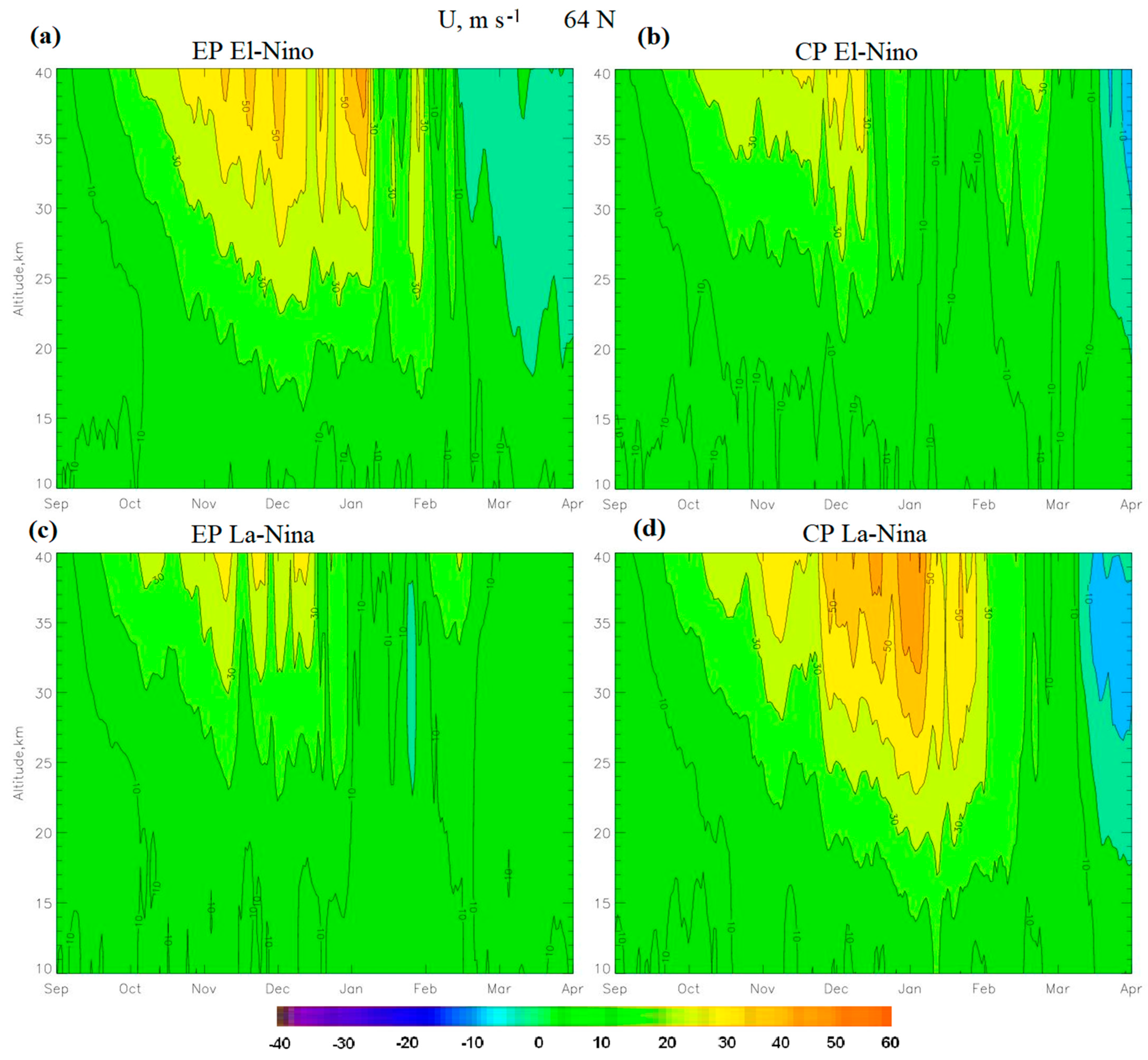
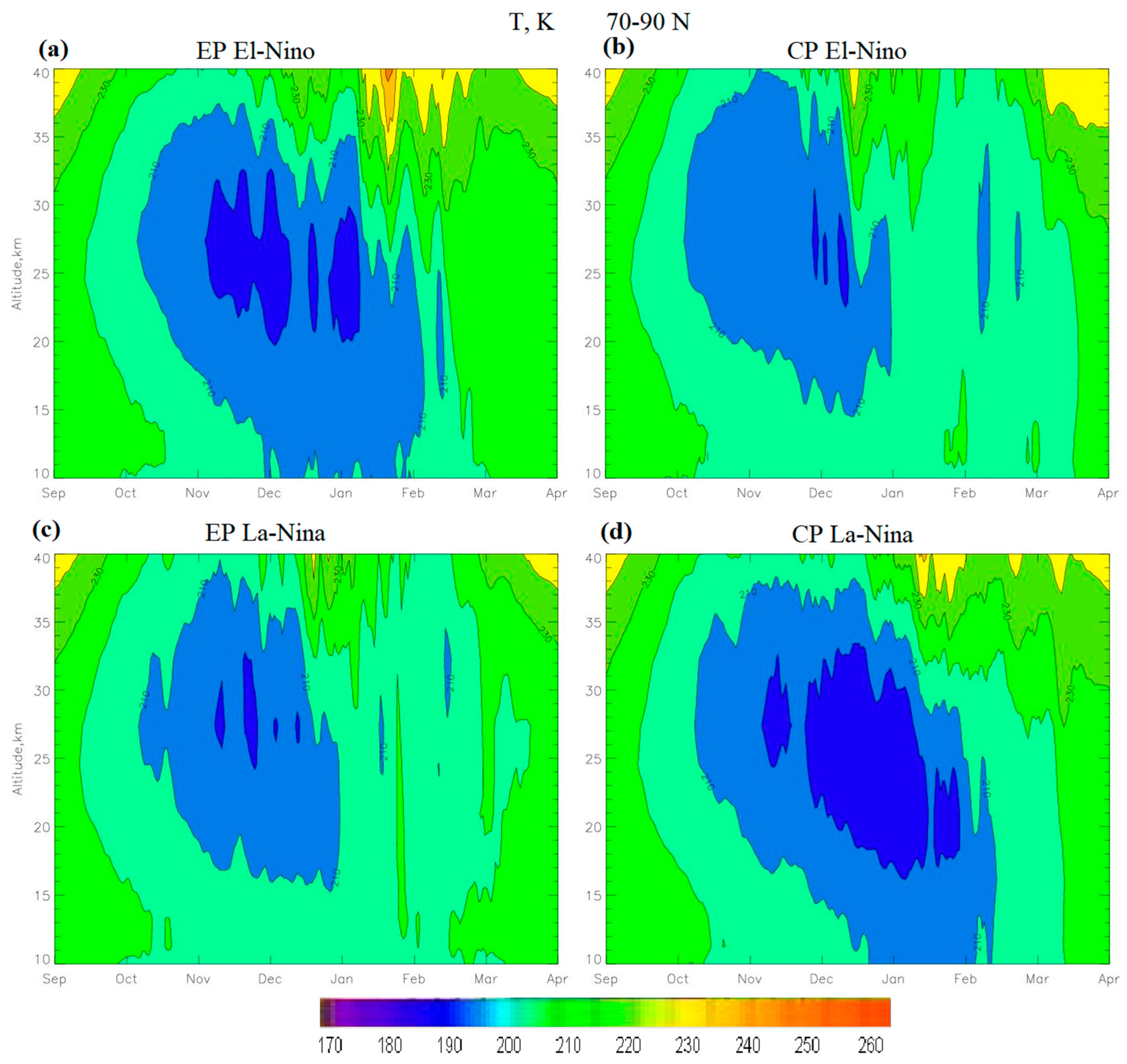
  • The El Niño phase leads to an increase in heat and mass fluxes into the stratosphere, which contributes to an increase in the SSW and a weakening of the PV. At the same time, it has been shown that during the CP El Niño, the SSW is stronger and occurs earlier than during the EP El Niño. As a result, the PV in the CP El Niño is weaker than in the EP El Niño.
  • The circulation processes during the La Niña phase depend on the type of La Niña. With CP La Niña, there is no SSW, as a result of which the PV is stable. During the EP La Niña, powerful SSWs are observed, which lead to a weakening of the PV. Analysis of the duration of ENSO phases showed that the longer the duration of an ENSO event, the stronger its influence. For example, the longer the El Niño lasts, the more powerful the SSW and the increase in total ozone associated with it.
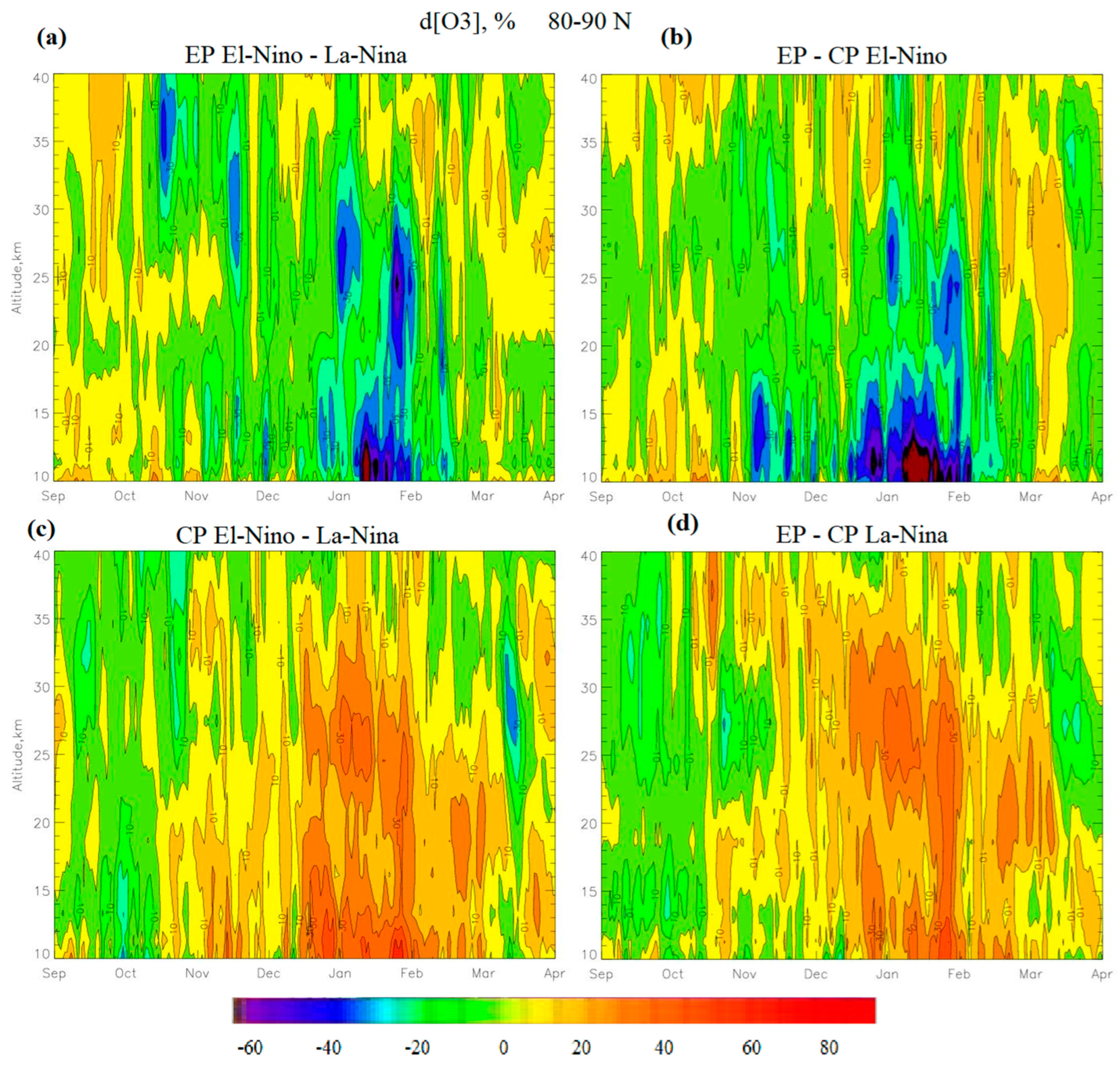
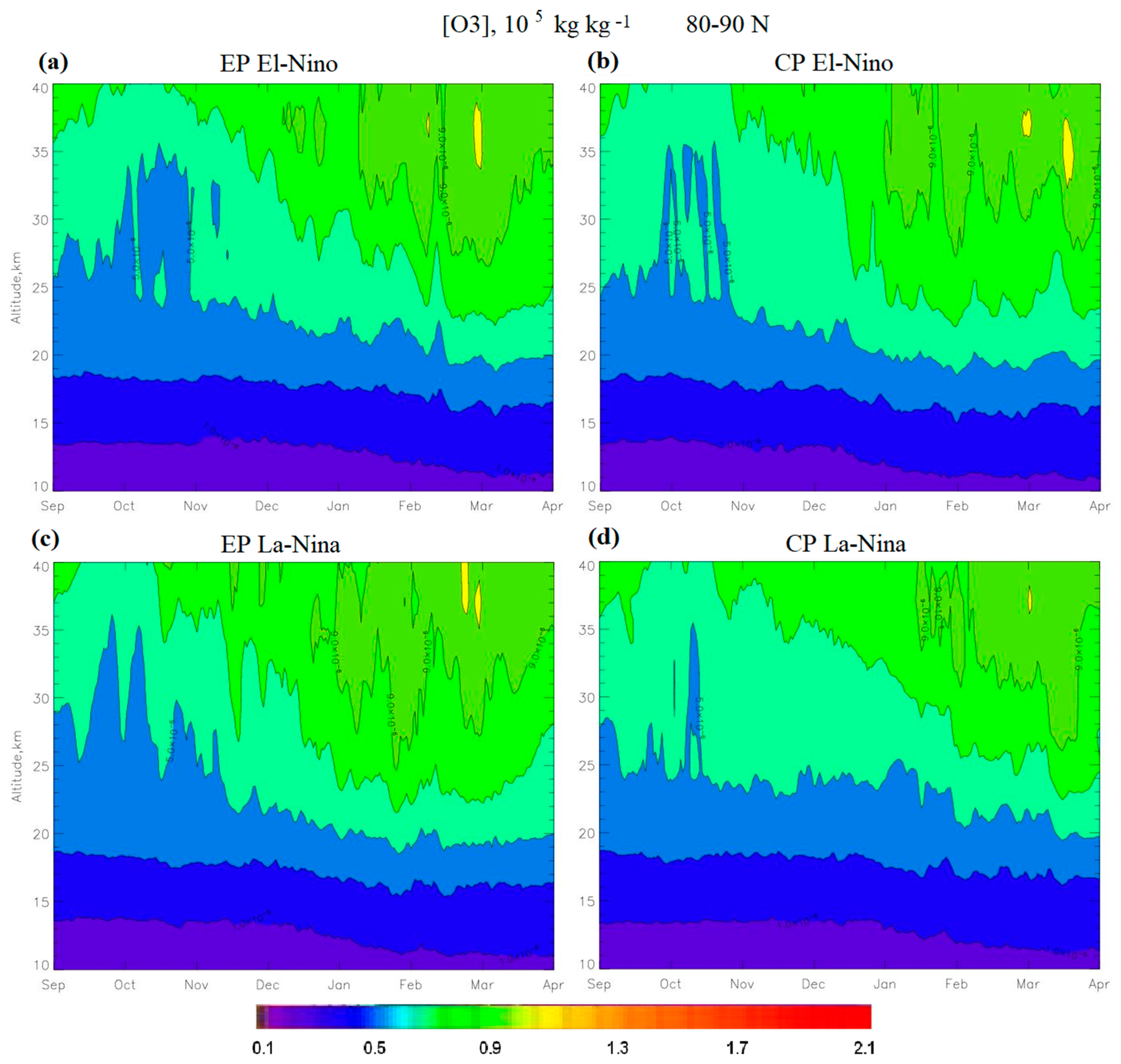
  • The largest increase in ozone occurs during CP El Niño and EP La Niña. During these phases, the SSWs are the most powerful and occur in January, leading to the destruction of the PV, which leads to an increase in the BD circulation. During EP El Niño, the SSW occurs in February, so the PV is more stable than during CP El Niño and EP La Niña, and the ozone concentration increases later and not as much as during CP El Niño and EP La Niña. At CP La Niña, there are no SSWs, the PV is stable, so the BD circulation is weak, and the ozone concentration decreases to the state of the ozone hole.
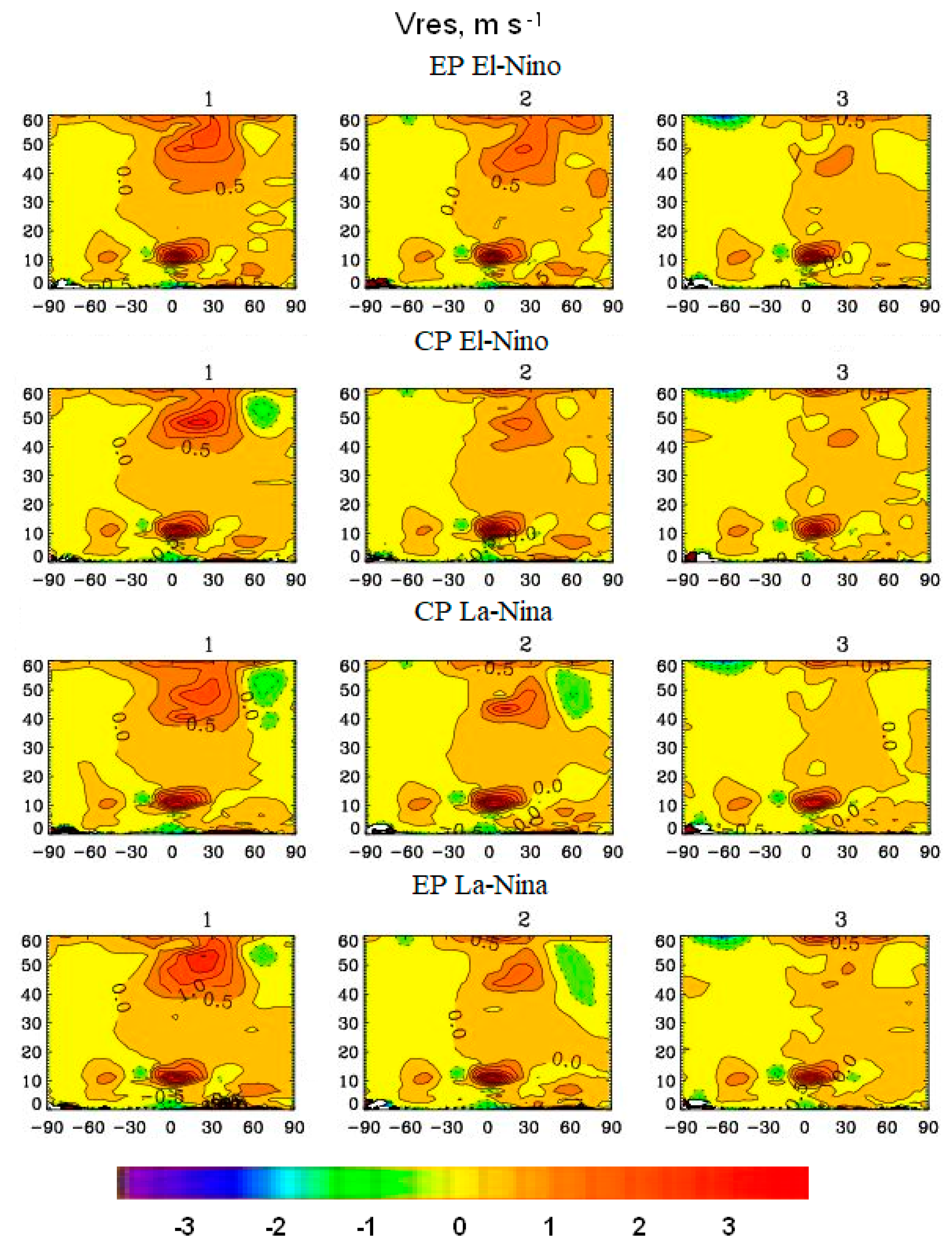
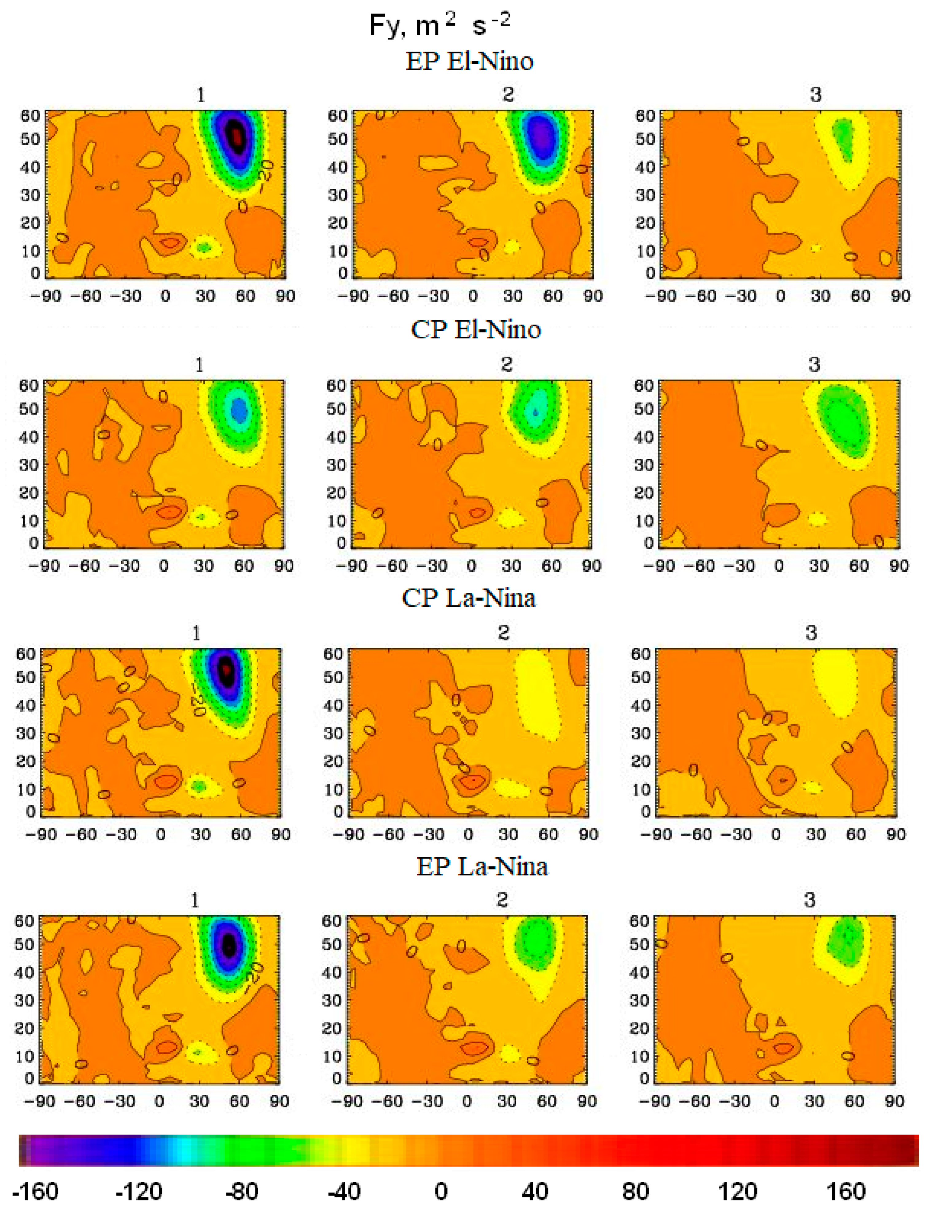
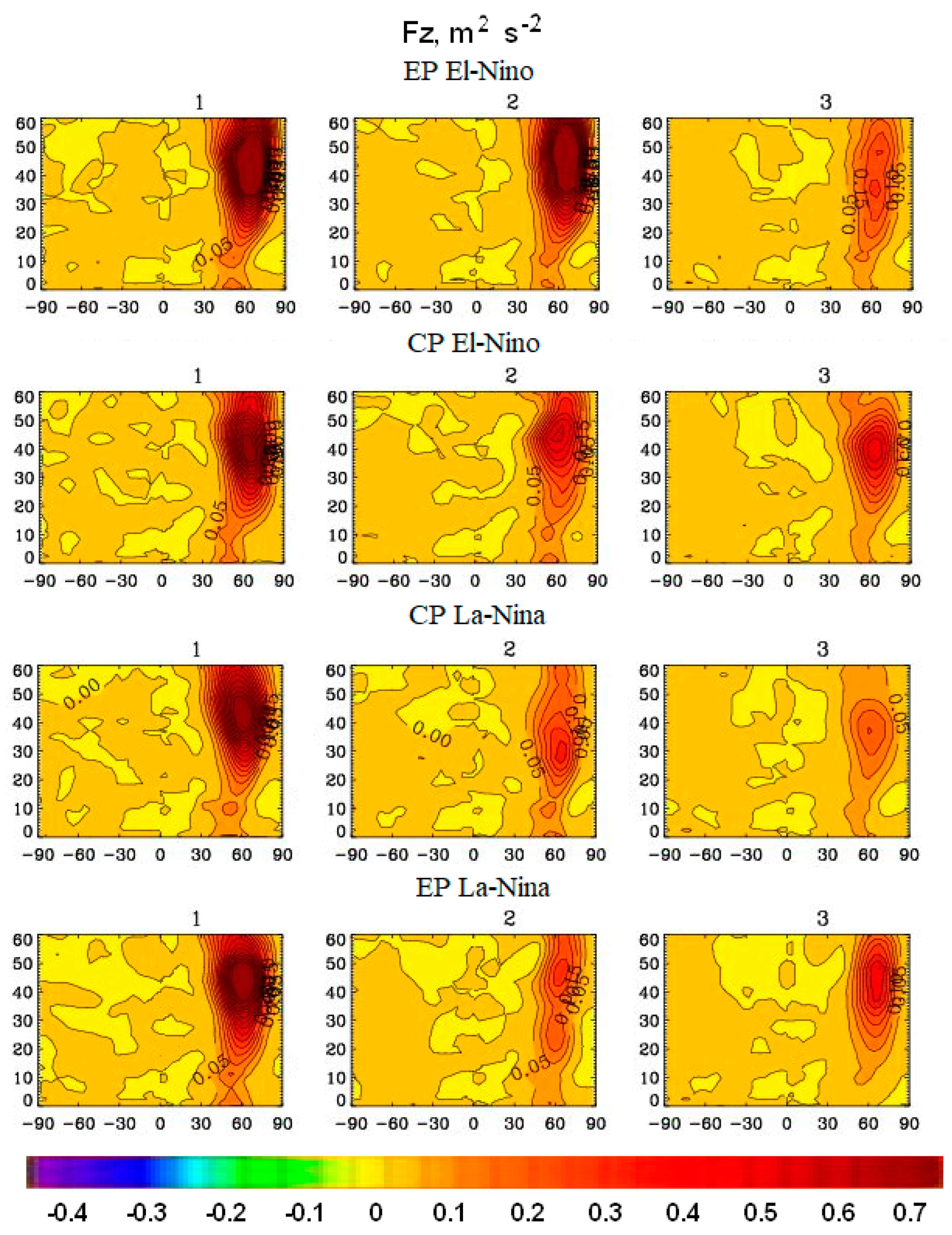
  • The largest intensification of the residual meridional circulation occurs at the El Niño phases of both types. At the EP La Niña phase, the residual meridional circulation in the Northern Hemisphere is intensified in February–March, while at CP La Niña, the residual circulation is not intensified. As for the wave activity flux, the greatest strengthening of the meridional and vertical components is observed at EP El Niño in February, also the wave activity flux strengthens at CP El Niño and EP La Niña, while at CP La Niña it weakens. Thus, the El Niño and EP La Niña phases contribute to the enhanced heat and mass transport through the residual circulation and wave activity flux, which contributes to the weakening of DWC and PV, strengthening of SSW and increase in total ozone.

Author Contributions

Conceptualization, S.P.S.; methodology, S.P.S.; formal analysis, A.R.J.; data curation, A.R.J.; writing—original draft preparation, A.R.J.; writing—review and editing, S.P.S.; visualization, A.R.J. All authors have read and agreed to the published version of the manuscript.

Funding

Work is executed at the Russian State Hydrometeorology University within the limits of the state task of the Ministry of Higher Education and Science of the Russian Federation (project No. FSZU-2023-0004). The change in gas structure of the atmosphere of the Arctic regions and Subarctic region was simulated with the support of the Russian Scientific Foundation (project No. 23-77-30008).

Data Availability Statement

The reanalysis data used in this article are available in the RSHU data service http://ra.rshu.ru/files/Jakovlev_Smyshlyaev_Meteorology_2024 (accessed on 15 January 2024).

Acknowledgments

We would like to thank the European Centre for Medium-Range Weather Forecasts (ECMWF) for providing the ERA5 Data Sets and NASA for providing the MERRA2 Data Set. The authors are grateful to the two anonymous referees for their attention to the manuscript and helpful and constructive comments.

Conflicts of Interest

The authors declare no conflict of interest.

References

  1. Czaja, A. Ocean-atmosphere coupling in midlatitudes: Does it invigorate or damp the storm track? In Proceedings of the ECMWF Seminar on Seasonal Prediction, Reading, UK, 3–7 September 2012; pp. 35–46. [Google Scholar]
  2. Bjerknes, J. Atmospheric teleconnections from the equatorial Pacific. Mon. Weather Rev. 1969, 97, 163–172. [Google Scholar] [CrossRef]
  3. Liu, Z.; Alexander, M. Atmospheric bridge, oceanic tunnel, and global climatic teleconnections. Rev. Geophys. 2007, 45, RG2005. [Google Scholar] [CrossRef]
  4. Graf, H.-F.; Zanchettin, D. Central Pacific El Niño, the “subtropical bridge”, and Eurasian climate. J. Geophys. Res. 2012, 117, D01102. [Google Scholar] [CrossRef]
  5. Frauen, C.; Dommenget, D.; Tyrrell, N.; Rezny, M.; Wales, S. Analysis of the Nonlinearity of El Niño–Southern Oscillation Teleconnections. J. Clim. 2014, 27, 6225–6244. [Google Scholar] [CrossRef]
  6. Zheleznova, I.V.; Gushchina, D.Y. The response of global atmospheric circulation to two types of El Niño. Russ. Meteorol. Hydrol. 2015, 40, 170–179. [Google Scholar] [CrossRef]
  7. Zheleznova, I.V.; Gushchina, D.Y. Circulation anomalies in the atmospheric centers of action during the Eastern Pacific and Central Pacific El Niño. Russ. Meteorol. Hydrol. 2016, 41, 760–769. [Google Scholar] [CrossRef]
  8. Zhou, X.; Li, J.P.; Xie, F.; Chen, Q.L.; Ding, R.Q.; Zhang, W.X.; Li, Y. Does Extreme El Nino Have a Different Effect on the Stratosphere in Boreal Winter Than Its Moderate Counterpart? J. Geophys. Res. 2018, 123, 3071–3086. [Google Scholar] [CrossRef]
  9. Zhou, X.; Chen, Q.; Wang, Z.; Xu, M.; Zhao, S.; Cheng, Z.; Feng, F. Longer duration of the weak stratospheric vortex during extreme El Niño events linked to spring Eurasian coldness. J. Geophys. Res. Atmos. 2020, 125, e2019JD032331. [Google Scholar] [CrossRef]
  10. Ashok, K.; Behera, S.K.; Rao, S.A.; Weng, H.; Yamagata, T. El Niño Modoki and its possible teleconnection. J. Geophys. Res. 2007, 112, C11007. [Google Scholar] [CrossRef]
  11. Capotondi, A.; Wittenberg, A.T.; Newman, M.; Di Lorenzo, E.; Yu, J.-Y.; Braconnot, P.; Cole, J.; Dewitte, B.; Giese, B.; Guilyardi, E.; et al. Understanding ENSO diversity. Bull. Am. Meteorol. Soc. 2015, 96, 921–938. [Google Scholar] [CrossRef]
  12. Timmermann, A.; An, S.-I.; Kug, J.-S.; Jin, F.-F.; Cai, W.; Capotondi, A.; Cobb, K.M.; Lengaigne, M.; McPhaden, M.J.; Stuecker, M.F.; et al. El Niño–Southern Oscillation complexity. Nature 2018, 559, 535–545. [Google Scholar] [CrossRef]
  13. Takahashi, K.; Dewitte, B. Strong and moderate nonlinear El Niño regimes. Clim. Dyn. 2016, 46, 1627–1645. [Google Scholar] [CrossRef]
  14. Yeh, S.-W.; Cai, W.; Min, S.-K.; McPhaden, M.J.; Dommenget, D.; Dewitte, B.; Collins, M.; Ashok, K.; An, S.I.; Yim, B.Y.; et al. ENSO atmospheric teleconnections and their response to greenhouse gas forcing. Rev. Geophys. 2018, 56, 185–206. [Google Scholar] [CrossRef]
  15. Taschetto, S.A.; Ummenhofer, C.C.; Stuecker, M.F.; Dommenget, D.; Ashok, K.; Rodrigues, R.R.; Yeh, S.-W. ENSO atmospheric teleconnections. In El Niño Southern Oscillation in a Changing Climate; McPhaden, M.J., Santoso, A., Cai, W., Eds.; AGU Monograph; American Geophysical Union: Washington, DC, USA, 2020. [Google Scholar]
  16. Calvo, N.; García-Herrera, R.; Garcia, R.R. The ENSO signal in the stratosphere. Ann. N. Y. Acad. Sci. 2008, 1146, 16–31. [Google Scholar] [CrossRef]
  17. Manzini, E. Atmospheric science: ENSO and the stratosphere. Nat. Geosci. 2009, 2, 749–750. [Google Scholar] [CrossRef]
  18. Domeisen, D.I.; Garfinkel, C.I.; Butler, A.H. The Teleconnection of El Niño Southern Oscillation to the Stratosphere. Rev. Geophys. 2019, 57, 5–47. [Google Scholar] [CrossRef]
  19. Jakovlev, A.R.; Smyshlyaev, S.P. Impact of the Southern Oscillation on Arctic Stratospheric Dynamics and Ozone Layer. Izv. Atmos. Ocean. Phys. 2019, 55, 86–99. [Google Scholar] [CrossRef]
  20. Pogoreltsev, A.I.; Savenkova, E.N.; Pertsev, N.N. Sudden Stratospheric Warmings: The Role of Normal Atmospheric Modes. Geomagn. Aeron. 2014, 54, 387–403. [Google Scholar] [CrossRef]
  21. Polvani, L.M.; Sun, L.; Butler, A.H.; Richter, J.H.; Deser, C. Distinguishing stratospheric sudden warmings from ENSO as key drivers of wintertime climate variability over the North Atlantic and Eurasia. J. Clim. 2017, 30, 1959–1969. [Google Scholar] [CrossRef]
  22. Baldwin, M.P.; Dunkerton, T.J. Propagation of the Arctic Oscillation from the stratosphere to the troposphere. J. Geophys. Res. 1999, 104, 430–937. [Google Scholar]
  23. Thompson, D.; Wallace, J. Observed linkages between Eurasian surface air temperature, the North Atlantic Oscillation, Arctic Sea level pressure and the stratospheric polar vortex. Geophys. Res. Lett. 1998, 25, 1297–1300. [Google Scholar] [CrossRef]
  24. Baldwin, M.P.; Dunkerton, T.J. Stratospheric harbingers of anomalous weather regimes. Science 2001, 294, 581–584. [Google Scholar] [CrossRef] [PubMed]
  25. Kuroda, K. Relationship between the Polar-Night Jet Oscillation and the Annular Mode. Geophys. Res. Lett. 2002, 29, 1240. [Google Scholar] [CrossRef]
  26. Li, Y.; Lau, N.-C. Influences of ENSO on stratospheric variability, and the descent of stratospheric perturbations into the lower troposphere. J. Clim. 2013, 26, 4725–4748. [Google Scholar] [CrossRef]
  27. Cheung, H.N.; Zhou, W.; Leung, M.Y.T.; Shun, C.M.; Lee, S.M.; Tong, H.W. A strong phase reversal of the Arctic Oscillation in midwinter 2015/2016: Role of the stratospheric polar vortex and tropospheric blocking. J. Geophys. Res. Atmos. 2016, 121, 13443–13457. [Google Scholar] [CrossRef]
  28. Manney, G.L.; Santee, M.L.; Rex, M.; Livesey, N.J.; Pitts, M.C.; Veefkind, P.; Nash, E.R.; Wohltmann, I.; Lehmann, R.; Froidevaux, L.; et al. Unprecedented Arctic ozone loss in 2011. Nature 2011, 478, 469. [Google Scholar] [CrossRef]
  29. Rao, J.; Garfinkel, C.I. Arctic Ozone Loss in March 2020 and Its Seasonal Prediction in CFSv2: A Comparative Study with the 1997 and 2011 Cases. J. Geophys. Res. Atmos. 2020, 125, e2020JD033524. [Google Scholar] [CrossRef]
  30. Garfinkel, C.I.; Hartmann, D.L. Different ENSO teleconnections and their effects on the stratospheric polar vortex. J. Geophys. Res. 2008, 113, D18114. [Google Scholar] [CrossRef]
  31. Baldwin, M.P.; O’Sullivan, D. Stratospheric effects of ENSO related tropospheric circulation anomalies. J. Clim. 1995, 8, 649–667. [Google Scholar] [CrossRef]
  32. Hoskins, B.J.; Karoly, D.J. The Steady Linear Response of a Spherical Atmosphere to Thermal and Orographic Forcing. J. Atmos. Sci. 1981, 38, 1179–1196. [Google Scholar] [CrossRef]
  33. Trenberth, K.E.; Branstator, G.W.; Karoly, D.; Kumar, A.; Lau, N.-C.; Ropelewski, C. Progress during TOGA in unferstanding and modeling global teleconnections associated with tropical sea surface temperatures. J. Geophys. Res. 1998, 103, 14291–14324. [Google Scholar] [CrossRef]
  34. Calvo, N.; Iza, M.; Hurwitz, M.M.; Manzini, E.; Peña-Ortiz, C.; Butler, A.H.; Cagnazzo, C.; Ineson, S.; Garfinkel, C.I. Northern Hemisphere stratospheric pathway of different El Niño flavors in CMIP5 models. J. Clim. 2017, 30, 4351–4371. [Google Scholar] [CrossRef]
  35. Garfinkel, C.I.; Hartmann, D.L. Effects of the El Niño Southern Oscillation and Quasi-Biennial Oscillation on polar temperatures in the stratosphere. J. Geophys. Res. 2007, 112, D19112. [Google Scholar] [CrossRef]
  36. Free, M.; Seidel, D.J. Observed El Niño—Southern Oscillation temperature signal in the stratosphere. J. Geophys. Res. 2009, 114, D23108. [Google Scholar] [CrossRef]
  37. Iza, M.; Calvo, N.; Manzini, E. The stratospheric pathway of La Niña. J. Clim. 2016, 29, 8899–8914. [Google Scholar] [CrossRef]
  38. Hurwitz, M.; Calvo, N.; Garfinkel, C.; Butler, A.; Ineson, S.; Cagnazzo, C.; Manzini, E.; Pena-Ortiz, C. Extra-tropical atmospheric response to ENSO in CMIP5 models. Clim. Dyn. 2014, 43, 3367–3375. [Google Scholar] [CrossRef]
  39. Xie, F.; Li, J.; Tian, W.; Feng, J.; Huo, Y. Signals of El Niño Modoki in the tropical tropopause layer and stratosphere. Atmos. Chem. Phys. 2012, 12, 5259–5273. [Google Scholar] [CrossRef]
  40. Garfinkel, C.I.; Hurwitz, M.M.; Waugh, D.W.; Butler, A.H. Are the teleconnections of central Pacific and eastern Pacific El Niño distinct in boreal wintertime? Clim. Dyn. 2012, 41, 1835–1852. [Google Scholar] [CrossRef]
  41. Weinberger, I.C.; White, I.; Oman, L. The Salience of Nonlinearities in the Boreal Winter Response to ENSO: Arctic Stratosphere and Europe. Clim. Dyn. 2019, 53, 4591–4610. [Google Scholar] [CrossRef]
  42. Kolennikova, M.; Gushchina, D. Revisiting the Contrasting Response of Polar Stratosphere to the Eastern and Central Pacific El Niños. Atmosphere 2022, 13, 682. [Google Scholar] [CrossRef]
  43. Xie, F.; Li, J.; Tian, W.; Zhang, J.; Sun, C. The relative impacts of El Nino Modoki, canonical El Nino, and QBO on tropical ozone changes since the 1980s. Environ. Res. Lett. 2014, 9, 064020. [Google Scholar] [CrossRef]
  44. Chandra, S.; Ziemke, J.R.; Min, W.; Read, W.G. Effects of 1997–1998 El Niño on tropospheric ozone and water vapor. Geophys. Res. Lett. 1998, 25, 3867–3870. [Google Scholar] [CrossRef]
  45. Cagnazzo, C.; Manzini, E.; Calvo, N.; Douglass, A.; Akiyoshi, H.; Bekki, S.; Chipperfield, M.; Dameris, M.; Deushi, M.; Fischer, A.M.; et al. Northern winter stratospheric temperature and ozone responses to ENSO inferred from an ensemble of chemistry climate models. Atmos. Chem. Phys. 2009, 9, 8935–8948. [Google Scholar] [CrossRef]
  46. Rieder, H.E.; Frossard, L.; Ribatet, M.; Staehelin, J.; Maeder, J.A.; Di Rocco, S.; Davison, A.C.; Peter, T.; Weihs, P.; Holawe, F. On the relationship between total ozone and atmospheric dynamics and chemistry at midlatitudes—Part 2: The effects of the El Niño/Southern Oscillation, volcanic eruptions and contributions of atmospheric dynamics and chemistry to long-term total ozone changes. Atmos. Chem. Phys. 2013, 13, 165–179. [Google Scholar] [CrossRef]
  47. Camp, C.; Roulston, M.; Yung, L. Temporal and spatial patterns of the interannual variability of total ozone in the tropics. J. Geophys. Res. 2013, 108, 4643. [Google Scholar] [CrossRef]
  48. Bonnimann, S.; Luterbacher, J.; Staehelin, J.; Svendby, T.M.; Hansen, G.; Svenøe, T. Extreme climate of the global troposphere and stratosphere 1940–1942 related to El Niño. Nature 2004, 431, 971–974. [Google Scholar] [CrossRef]
  49. Zhang, J.; Tian, W.; Wang, Z.; Xie, F.; Wang, F. The influence of ENSO on Northern mid-latitude ozone during the winter to spring transition. J. Clim. 2015, 28, 4774–4793. [Google Scholar] [CrossRef]
  50. Gettelman, A.; Randel, W.; Massie, S.; Wu, F. El Niño as a natural experiment for studying the tropical tropopause region. J. Clim. 2001, 14, 3375–3392. [Google Scholar] [CrossRef]
  51. Fusco, A.C.; Salby, M.L. Interannual variations of total ozone and their relationship to variations of planetary wave activity. J. Clim. 1999, 12, 1619–1629. [Google Scholar] [CrossRef]
  52. Randel, W.J.; Wu, F.; Stolarski, R. Changes in column ozone correlated with the stratospheric EP fux. J. Meteorol. Soc. Jpn. 2002, 80, 849–862. [Google Scholar] [CrossRef]
  53. Weber, M.; Dhomse, S.; Wittrock, F.; Richter, A.; Sinnhuber, B.-M.; Burrows, J.P. Dynamical control of NH and SH winter/spring total ozone from GOME observations in 1995–2002. Geophys. Res. Lett. 2003, 30, 1583. [Google Scholar] [CrossRef]
  54. Xie, F.; Li, J.; Tian, W.; Zhang, J. A connection from Arctic stratospheric ozone to El Niño-Southern oscillation. Environ. Res. Lett. 2016, 11, 124026. [Google Scholar] [CrossRef]
  55. Koval, A.V. Calculation of the Residual Mean Meridional Circulation According to the Middle and Upper Atmosphere Model. Uchonie Zap. RSHU 2019, 55, 25–32. (In Russian) [Google Scholar] [CrossRef]
  56. Brewer, A.W. Evidence for a world circulation provided by the measurements of helium and water vapor distribution in the stratosphere. Quart. J. Roy. Meteor. Soc. 1949, 75, 351–363. [Google Scholar] [CrossRef]
  57. Dobson, G.M.B. Origin and distribution of the polyatomic molecules in the atmosphere. Proc. R. Soc. Lond. Ser. A 1956, 236, 187–193. [Google Scholar]
  58. Shepherd, T.G. Transport in the middle atmosphere. J. Meteor. Soc. Jpn. 2007, 85B, 165–191. [Google Scholar] [CrossRef]
  59. Lubis, S.W.; Silverman, V.; Matthes, K.; Harnik, N.; Omrani, N.E.; Wahl, S. How Does Downward Planetary Wave Coupling Affect Polar Stratospheric Ozone in the Arctic Winter Stratosphere? Atmos. Chem. Phys. 2017, 17, 2437–2458. [Google Scholar] [CrossRef]
  60. de La Cámara, A.; Abalos, M.; Hitchcock, P.; Calvo, N.; Garcia, R.R. Response of Arctic ozone to sudden stratospheric warmings. Atmos. Chem. Phys. 2018, 18, 16499–16513. [Google Scholar] [CrossRef]
  61. Lubis, S.W.; Matthes, K.; Omrani, N.E.; Harnik, N.; Wahl, S. Influence of the Quasi-Biennial Oscillation and Sea Surface Temperature Variability on Downward Wave Coupling in the Northern Hemisphere. J. Atmos. Sci. 2016, 73, 1943–1965. [Google Scholar] [CrossRef]
  62. Silverman, V.; Harnik, N.; Matthes, K.; Lubis, S.W.; Wahl, S. Radiative effects of ozone waves on the Northern Hemisphere polar vortex and its modulation by the QBO. Atmos. Chem. Phys. 2018, 18, 6637–6659. [Google Scholar] [CrossRef]
  63. Silverman, V.; Lubis, S.W.; Harnik, N.; Matthes, K. A Synoptic View of the Onset of the Midlatitude QBO Signal. J. Atmos. Sci. 2021, 78, 3759–3780. [Google Scholar] [CrossRef]
  64. Richter, J.H.; Matthes, K.; Calvo, N.; Gray, L.J. Influence of the quasi-biennial oscillation and El Niño–Southern Oscillation on the frequency of sudden stratospheric warmings. J. Geophys. Res. 2011, 116, D2011. [Google Scholar] [CrossRef]
  65. Palmeiro, F.M.; García-Serrano, J.; Ruggieri, P.; Batté, L.; Gualdi, S. On the influence of ENSO on sudden stratospheric warmings. J. Geophys. Res. Atmos. 2023, 128, e2022JD037607. [Google Scholar] [CrossRef]
  66. Weather and Climate Change/Met Office. Available online: https://www.metoffice.gov.uk/hadobs/hadgem_sst/data/download.html (accessed on 20 March 2021).
  67. Kennedy, J. Uncertainties in Sea-Surface Temperature Measurements [Electronic Resource]; Met Office Hadley Centre, FitzRoy Road: Exeter, UK, 2008. Available online: https://icoads.noaa.gov/climar3/c3poster-pdfs/S1P1-Kennedy.pdf (accessed on 15 January 2024).
  68. Donlon, C.J.; Martin, M.; Stark, J.; Roberts-Jones, J.; Fiedler, E.; Wimmer, W. The Operational Sea Surface Temperature and Sea Ice Analysis (OSTIA) system. Remote Sens. Environ. 2011, 116, 140–158. [Google Scholar] [CrossRef]
  69. Smyshlyaev, S.P.; Pogoreltsev, A.I.; Drobashevskaya, E.A.; Galin, V.Y. Influence of wave activity on the conposition of the polar stratosphere. Geomagn. Aeron. 2016, 56, 95–109. [Google Scholar] [CrossRef]
  70. Butchart, N. The Brewer-Dobson circulation. Rev. Geophys. 2014, 52, 157–184. [Google Scholar] [CrossRef]
  71. Plumb, R.A. On the Three-Dimensional Propagation of Stationary Waves. J. Atmos. Sci. 1985, 42, 217–229. [Google Scholar] [CrossRef]
  72. Dee, D.P.; Uppala, S.M.; Simmons, A.J.; Berrisford, P.; Poli, P.; Kobayashi, S.; Andrae, U.; Balmaseda, M.A.; Balsamo, G.; Bauer, P.; et al. The ERA-Interim reanalysis: Configuration and performance of the data assimilation system. Q. J. R. Meteorol. Soc. 2011, 137, 553–597. [Google Scholar] [CrossRef]
  73. Gelaro, R.; McCarty, W.; Suarez, M.J.; Todling, R.; Molod, A.; Takacs, L.; Randles, C.; Darmenov, A.; Bosilovich, M.; Reichle, R.; et al. The Modern-Era Retrospective Analysis for Research and Applications, Version 2 (MERRA-2). J. Clim. 2017, 30, 5419–5454. [Google Scholar] [CrossRef]
  74. Jakovlev, A.R.; Smyshlyaev, S.P. The numerical simulations of global influence of ocean and El-Nino—La-Nina on structure and composition of atmosphere. Uchonie Zap. RSHU 2017, 49, 58–72. (In Russian) [Google Scholar]
  75. Jakovlev, A.R.; Smyshlyaev, S.P. Simulation of influence of ocean and El-Nino—Southern oscillation phenomenon on the structure and composition of the atmosphere. IOP Conf. Ser. Earth Environ. Sci. 2019, 386, 012021. [Google Scholar] [CrossRef]
  76. Jakovlev, A.R.; Smyshlyaev, S.P. Numerical Simulation of World Ocean Effects on Temperature and Ozone in the Lower and Middle Atmosphere. Russ. Meteorol. Hydrol. 2019, 44, 594–602. [Google Scholar] [CrossRef]
  77. Jakovlev, A.R.; Smyshlyaev, S.P.; Galin, V.Y. Interannual Variability and Trends in Sea Surface Temperature, Lower and Middle Atmosphere Temperature at Different Latitudes for 1980–2019. Atmosphere 2021, 12, 454. [Google Scholar] [CrossRef]
  78. Garcia-Herrera, R.; Calvo, N.; Garcia, R.R.; Giorgetta, M.A. Propagation of ENSO temperature signals into the middle atmosphere: A comparison of two general circulation models and ERA-40 reanalysis data. J. Geophys. Res. 2006, 111, D06101. [Google Scholar] [CrossRef]
  79. Sassi, F.; Kinnison, D.; Bolville, B.A.; Garcia, R.R.; Roble, R. Effect of El-Nino Southern Oscillation on the dynamical, thermal, and chemical structure of the middle atmosphere. J. Geophys. Res. 2004, 109, D17108. [Google Scholar] [CrossRef]
  80. Scott, R.; Polvani, L. Internal variability of the winter stratosphere. J. Atmos. Sci. 2006, 63, 2758–2778. [Google Scholar] [CrossRef]
  81. Karpechko, A.; Perlwitz, J.; Manzini, E. A model study of tropospheric impacts of the Arctic ozone depletion 2011. J. Geophys. Res. 2014, 119, 7999–8014. [Google Scholar] [CrossRef]
  82. Pogoreltsev, A.I.; Savenkova, E.N.; Aniskina, O.G.; Ermakova, T.S.; Chen, W.; Wei, K. Interannual and intraseasonal variability of stratospheric dynamics and stratosphere-troposphere coupling during northern winter. J. Atmos. Sol.-Terr. Phys. 2015, 136, 187–200. [Google Scholar] [CrossRef]
  83. Gushchina, D.; Kolennikova, M.; Dewitte, B.; Yeh, S.-W. On the relationship between ENSO diversity and the ENSO atmospheric teleconnection to high-latitudes. Int. J. Climatol. 2021, 42, 1303–1325. [Google Scholar] [CrossRef]
  84. Plumb, R.A. On the seasonal cycle of stratospheric planetary waves. Pure Appl. Geophys. 1989, 130, 233–242. [Google Scholar] [CrossRef]
  85. Rao, J.; Ren, R. Modeling study of the destructive interference between the tropical Indian Ocean and eastern Pacific in their forcing in the southern winter extratropical stratosphere during ENSO. Clim. Dyn. 2020, 54, 2249–2266. [Google Scholar] [CrossRef]
  86. Karoly, D.J. Southern Hemisphere circulation features associated with El Ni-ño-Southern Oscillation events. J. Clim. 1989, 2, 1239–1252. [Google Scholar] [CrossRef]
  87. Smith, K.L.; Kushner, P.J. Linear interference and the initiation of extratropical stratosphere-troposphere interactions. J. Geophys. Res. 2012, 117, D13107. [Google Scholar] [CrossRef]
  88. Rao, J.; Ren, R. A decomposition of ENSO’s impacts on the northern winter stratosphere: Competing effect of SST forcing in the tropical Indian Ocean. Clim. Dyn. 2016, 46, 3689–3707. [Google Scholar] [CrossRef]
  89. Rao, J.; Garfinkel, C.I.; Ren, R. Modulation of the northern winter stratospheric El Niño-Southern Oscillation teleconnection by the PDO. J. Clim. 2019, 32, 5761–5783. [Google Scholar] [CrossRef]
  90. Ayarzagüena, B.; Ineson, S.; Dunstone, N.; Baldwin, M.; Scaife, A. Intraseasonal Effects of El Niño–Southern Oscillation on North Atlantic Climate. J. Clim. 2018, 31, 8861–8873. [Google Scholar] [CrossRef]
  91. Palmeiro, F.; Iza, M.; Barriopedro, D.; Calvo, N.; Garcнa-Herrera, R. The complex behavior of El Niсo winter 2015–2016. Geophys. Res. Lett. 2017, 44, 2902–2910. [Google Scholar] [CrossRef]
  92. Bell, C.J.; Gray, L.J.; Charlton-Perez, A.J.; Joshi, M.M.; Scaife, A.A. Stratospheric communication of El Niсo teleconnections to European winter. J. Clim. 2009, 22, 4083–4096. [Google Scholar] [CrossRef]
  93. Domeisen, D.I.V.; Butler, A.H.; Frцhlich, K.; Bittner, M.; Mьller, W.; Baehr, J. Seasonal predictability over Europe arising from El Niсo and stratospheric variability in the MPI-ESM Seasonal Prediction System. J. Clim. 2015, 28, 256–271. [Google Scholar] [CrossRef]
  94. Garfinkel, C.I.; Butler, A.H.; Waugh, D.W.; Hurwitz, M.M.; Polvani, L.M. Why might stratospheric sudden warmings occur with similar frequency in El Nino and La Nina winters. J. Geophys. Res. 2012, 117, D19106. [Google Scholar] [CrossRef]
  95. Taguchi, M.; Hartmann, D.L. Increased occurrence of stratospheric sudden warmings during El Niсo as simulated by WACCM. J. Clim. 2006, 19, 332. [Google Scholar] [CrossRef]
  96. Kinoshita, T.; Tomikawa, Y.; Sato, K. On the Three-Dimensional Residual Mean Circulation and Wave Activity Flux of the Primitive Equations. J. Meteorol. Soc. Jpn. 2010, 88, 373–394. [Google Scholar] [CrossRef]
Figure 1. SST anomalies in the region of 5 S–5 N, 170 W–120 W (green), 160 E–150 W (red), 150 W–90 W (blue) according to ERA5 (a) and Met Office (b). The ENSO CP type is marked with a “+” sign, and the EP type is marked with a “#” sign.
Meteorology 03 00002 g001
Figure 2. Total ozone column in the Arctic (70–90 N latitude) on average for January–March (a), January (b), February (c), March (d) according to ERA5 (blue) and MERRA2 (red). At the same time, CP El Niño, EP El Niño, CP La Niña and EP La Niña are marked with the signs “+”, “#”, “$” and “@”, respectively.
Meteorology 03 00002 g002
Figure 3. Air temperature in the Arctic stratosphere (70–90 N, 15–30 km on average for January–March (a), for January (b), for February (c), for March (d) according to ERA5 (blue) and MERRA2 (red), with CP El Niño, EP El Niño, CP La Niña and EP La Niña marked with “+”, “#”, “$” and “@”, respectively.
Meteorology 03 00002 g003
Figure 4. Zonal average daily vertical profiles of zonal wind speed at 64 N according to MERRA2 reanalysis for years with EP El Niño (a), for years with CP El Niño (b), for years with EP La Niña (c), over the years with CP La Niña (d).
Meteorology 03 00002 g004
Figure 5. Zonal average daily vertical profiles of ozone anomalies in % at 80–90 N according to MERRA2 reanalysis. At the (a) are the relative differences in ozone concentrations between years with the El Niño and La Niña phases with the EP type, at the (c) are the relative differences between the years with the El Niño and La Niña phases with the CP type, at the (b) are the relative differences between years with the El Niño phase of the EP and CP types, and at the (d) are the relative differences between the years with the La Niña phase of the EP and CP types.
Meteorology 03 00002 g005
Figure 6. Zonal average daily vertical profiles of ozone mixing ratio at 80–90 N according to MERRA2 reanalysis for years with EP El Niño (a), for years with CP El Niño (b), for years with EP La Niña (c), over the years since CP La Niña (d).
Meteorology 03 00002 g006
Figure 7. Zonal mean daily vertical air temperature profiles at 70–90 N according to MERRA2 reanalysis data for years with EP El Niño (a), for years with CP El Niño (b), for years with EP La Niña (c), for years since CP La Niña (d).
Meteorology 03 00002 g007
Figure 8. Zonal average profiles of residual meridional circulation for January (1), February (2) and March (3).
Meteorology 03 00002 g008
Figure 9. Zonal average profiles of meridional component of Plumb flux for January (1), February (2) and March (3).
Meteorology 03 00002 g009
Figure 10. Zonal average profiles of vertical component of Plumb flux for January (1), February (2) and March (3).
Meteorology 03 00002 g010
Table 1. El Niño and La Niña types [18], SST anomalies and their duration in months in the regions 160 E–150 W (Nino3), 170 W–120 W (Nino3.4), 150 W–90 W (Nino4), as well as anomalies in the total ozone content and air temperature in the Arctic stratosphere (70–90 N). Red color—EP El Niño, yellow color—CP El Niño, green color—EP La Niña, blue color—CP La Niña, grey color—ENSO of unspecified type, pink color—TO3 anomaly >25 DU, cyan color—TO3 anomaly <−25 DU.
YearENSO PhaseCP/EPSST Anomaly (Duration of the Period with an SST Anomaly of More than 0.5 or −0.5, Months)TO3 Anomaly 70–90 N January–MarchT Anomaly 70–90 N 15–30 km January–March
160 E–150 W170 W–120 W150 W–90 WMERRA2ERA5MERRA2ERA5
1980El-NiñoEP0.30.5 (4)0.5 (4)154−0.9−0.5
1981Neutral 0.1−0.3−0.11330.71.0
1982Neutral −0.3−0.2−0.1114−1.8−1.5
1983El-NiñoEP0.5 (5)2.0 (13)2.2 (16)−14−30.00.3
1984La-NiñaCP−0.7 (12)−0.5 (12)−0.7 (3)−100.70.8
1985La-NiñaEP−0.7 (17)−1.0 (14)−1.0 (9)29395.45.4
1986Neutral −0.7 (3)−0.4−0.4−12−19−1.1−1.0
1987El-NiñoEP0.5 (5) 1.1 (17)0.9 (16)39437.47.3
1988El-NiñoEP0.7 (8)0.9 (17)1.1 (16)312−4.1−4.0
1989La-NiñaCP−1.5 (16)−1.5 (16)−1.6 (15)1281.61.7
1990Neutral −0.3−0.3−0.3−26−33−4.9−4.6
1991Neutral 0.4−0.10.220132.52.4
1992El-NiñoCP/EP0.5 (7)1.0 (8)0.8 (9)−18−122.72.9
1993Neutral 0.1−0.20.0−42−30−3.3−3.0
1994Neutral 0.30.10.2−18−2−3.2−3.0
1995El-NiñoCP0.7 (6)0.7 (6)0.8 (5)−198−1.2−0.9
1996La-NiñaEP−0.2−0.6 (6)−0.6 (7)−53−59−5.8−5.5
1997Neutral −0.1−0.4−0.5 (4)−53−42−11.0−10.3
1998El-NiñoEP0.7 (8)2.0 (11)2.2 (13)511.41.4
1999La-NiñaCP−1.0 (24)−0.6 (25)−0.7 (5)23323.03.0
2000La-NiñaCP−1.1 (24)−1.1 (25)−1.2 (12)−46−51−6.2−6.3
2001La-NiñaEP/CP−0.6 (6)−0.7 (6)−0.6 (4)32303.73.4
2002Neutral 0.1−0.3−0.5 (5)22244.23.9
2003El-NiñoCP0.7 (10)0.8 (10)0.9 (5)2−92.72.5
2004Neutral 0.30.20.333234.03.7
2005El-NiñoCP0.6 (7)0.5 (6)0.4−24−28−3.0−3.3
2006La-NiñaEP−0.1−0.7 (5)−0.7 (6)41345.24.8
2007El-NiñoEP0.5 (4)0.6 (5)0.7 (5)−11−18−2.6−2.5
2008La-NiñaCP−1.1 (11)−1.1 (11)−1.1 (12)1−81.61.7
2009La-NiñaCP−0.6 (4)−0.5 (5)−0.5 (4)35265.45.3
2010El-NiñoCP1.0 (9)1.0 (10)1.0 (11)34284.84.7
2011La-NiñaCP−1.4 (21)−1.5 (12)−1.5 (10)−52−59−9.6−9.6
2012La-NiñaCP−0.8 (21)−0.8 (8)−0.9 (5)1561.81.6
2013Neutral 0.2−0.1−0.6 (4)31253.93.6
2014Neutral −0.1−0.2−0.2−14−17−0.6−0.7
2015El-NiñoCP0.5 (19)0.5 (19)0.5 (3)1422−1.9−2.0
2016El-NiñoEP1.2 (19)2.1 (19)2.0 (13)−15−130.40.2
2017Neutral −0.2−0.3−0.47171.61.5
2018La-NiñaEP−0.2−0.7 (7)−0.7 (8)8143.12.9
2019El-NiñoCP0.6 (16)0.5 (9)0.6 (7)42542.42.1
2020Neutral 0.5 (16)0.10.3−70−68−9.3−9.3
Table 2. Total ozone content and air temperature in the Arctic stratosphere (70–90 N) for January, February and March according to ERA5 and MERRA2 reanalysis data. Red color—EP El Niño, yellow color—CP El Niño, green color—EP La Niña, blue color—CP La Niña, grey color—ENSO of unspecified type, pink color—TO3 anomaly >25 DU, cyan color—TO3 anomaly <−25 DU.
YearENSO PhaseCP/EPTO3 Anomaly 70–90 N January–MarchT Anomaly 70–90 N 15–30 km January–March
JanuaryFebruaryMarchJanuaryFebruaryMarch
MERRA2ERA5MERRA2ERA5MERRA2ERA5
1980El-NiñoEP−5−215−84641−6.4−4.07.9
1981Neutral −14−2725152821−6.75.23.6
1982Neutral 1231041260.8−2.0−4.1
1983El-NiñoEP−35−14−16−6810−5.60.45.3
1984La-NiñaCP−34−32−11−84339−7.2−1.010.6
1985La-NiñaEP42451327334413.20.82.3
1986Neutral −11−21−34−4085−1.5−6.14.2
1987El-NiñoEP1518748326287.313.61.5
1988El-NiñoEP125−22−183031−3.6−12.53.5
1989La-NiñaCP−35−351425856−9.13.010.8
1990Neutral −22−29−12−21−44−48−6.3−1.1−7.1
1991Neutral 8−4342718161.36.7−0.6
1992El-NiñoCP/EP−21−1−19−14−14−203.52.22.4
1993Neutral −42−10−44−34−39−45−7.8−4.62.4
1994Neutral −522−29−8−20−193.6−7.9−5.3
1995El-NiñoCP1523−1724−54−210.12.3−5.9
1996La-NiñaEP−37−49−68−71−54−57−7.3−9.2−0.8
1997Neutral −1637−46−59−98−104−3.8−12.9−16.2
1998El-NiñoEP113−2−1505.70.1−1.6
1999La-NiñaCP1231112146453.9−2.47.4
2000La-NiñaCP−53−51−49−59−34−44−8.7−8.2−1.6
2001La-NiñaEP/CP−2−757554041−3.512.22.4
2002Neutral 30322938959.24.5−1.0
2003El-NiñoCP6−5−4−162−55.71.41.1
2004Neutral 575135226−314.44.1−6.5
2005El-NiñoCP−27−33−42−46−2−7−8.7−6.56.1
2006La-NiñaEP48345854161612.07.5−3.9
2007El-NiñoEP2−12−6−15−28−28−3.0−1.7−3.0
2008La-NiñaCP−6−21−2−12128−4.02.86.1
2009La-NiñaCP11−2685926202.914.2−0.7
2010El-NiñoCP153554832310.211.13.2
2011La-NiñaCP−8−22−52−60−96−96−4.6−11.3−12.7
2012La-NiñaCP10−321111593.52.8−0.8
2013Neutral 463437359514.14.0−6.5
2014Neutral −6−18−24−27−13−7−3.8−1.13.0
2015El-NiñoCP4038716−4135.1−4.9−5.8
2016El-NiñoEP−29−30−43−412732−8.0−3.212.2
2017Neutral 3111122718−2.35.21.9
2018La-NiñaEP−25−1915233238−4.98.45.8
2019El-NiñoCP77873246172916.3−0.5−8.7
2020Neutral −29−31−71−68−109−105−6.3−11.0−10.7
Table 3. Selection of years with low (anomaly less than −25 DU) and high (anomaly more than 25 DU) total ozone at 70–90 N. for the period from January to March, as well as for January, February and March, depending on the phase of the ENSO.
MonthTotal Ozone Column Anomaly on 70–90 NNeutralEP El-NiñoCP El-NiñoEP La-NiñaCP La-Niña
January–March<−25 DU1990, 1993, 1997, 2020
4 years
0 years2005
1 year
1996
1 year
2000, 2011
2 years
>25 DU2004, 2013
2 years
1987
1 year
2010, 2019
2 years
1985, 2006
2 years
1999, 2009
2 years
January<−25 DU1981 (ERA5), 1990 (ERA5), 1993 (MERRA2), 2020
4 Years
1983 (MERRA2), 2016
2 years
2005
1 year
1996, 2018 (MERRA2)
2 years
1984, 1989. 2000
3 years
>25 DU1997 (ERA5), 2002, 2004, 2013
4 years
1988 (ERA5)
1 year
2015, 2019
2 years
1985, 2006
2 years
1999 (ERA5)
1 year
February<−25 DU1986, 1993, 1994 (MERRA2), 1997, 2014, 2020
6 years
2016
1 year
2005
1 year
1996
1 year
2000, 2011
2 years
>25 DU1981 (MERRA2), 1991, 2002, 2004 (MERRA2), 2013
5 years
1987
1 year
2010, 2019
2 years
1985 (ERA5), 2006
2 years
2009
1 year
March<−25 DU1990, 1993, 1997, 2020
4 years
2007
1 year
1995 (MERRA2)
1 year
1996
1 year
2000, 2011
2 years
>25 DU1981 (MERRA2)
1 year
1980, 1987, 1988, 2016
4 years
2010, 2019 (ERA5)
2 years
1985, 2018
2 years
1984, 1999, 2009 (MERRA2)
3 years
Disclaimer/Publisher’s Note: The statements, opinions and data contained in all publications are solely those of the individual author(s) and contributor(s) and not of MDPI and/or the editor(s). MDPI and/or the editor(s) disclaim responsibility for any injury to people or property resulting from any ideas, methods, instructions or products referred to in the content.

