

A Data-Driven Study of the Drivers of Stratospheric Circulation via Reduced Order Modeling and Data Assimilation

 , , , and
Abstract
:1. Introduction
1.1. General Background
- The interaction with waves propagating up from the troposphere;
- Differential radiative heating.
1.2. Data Assimilation and Reduced-Order Models
1.3. Our Main Focus
1.4. Outline of the Paper
2. Materials and Methods
2.1. Ruzmaikin Model
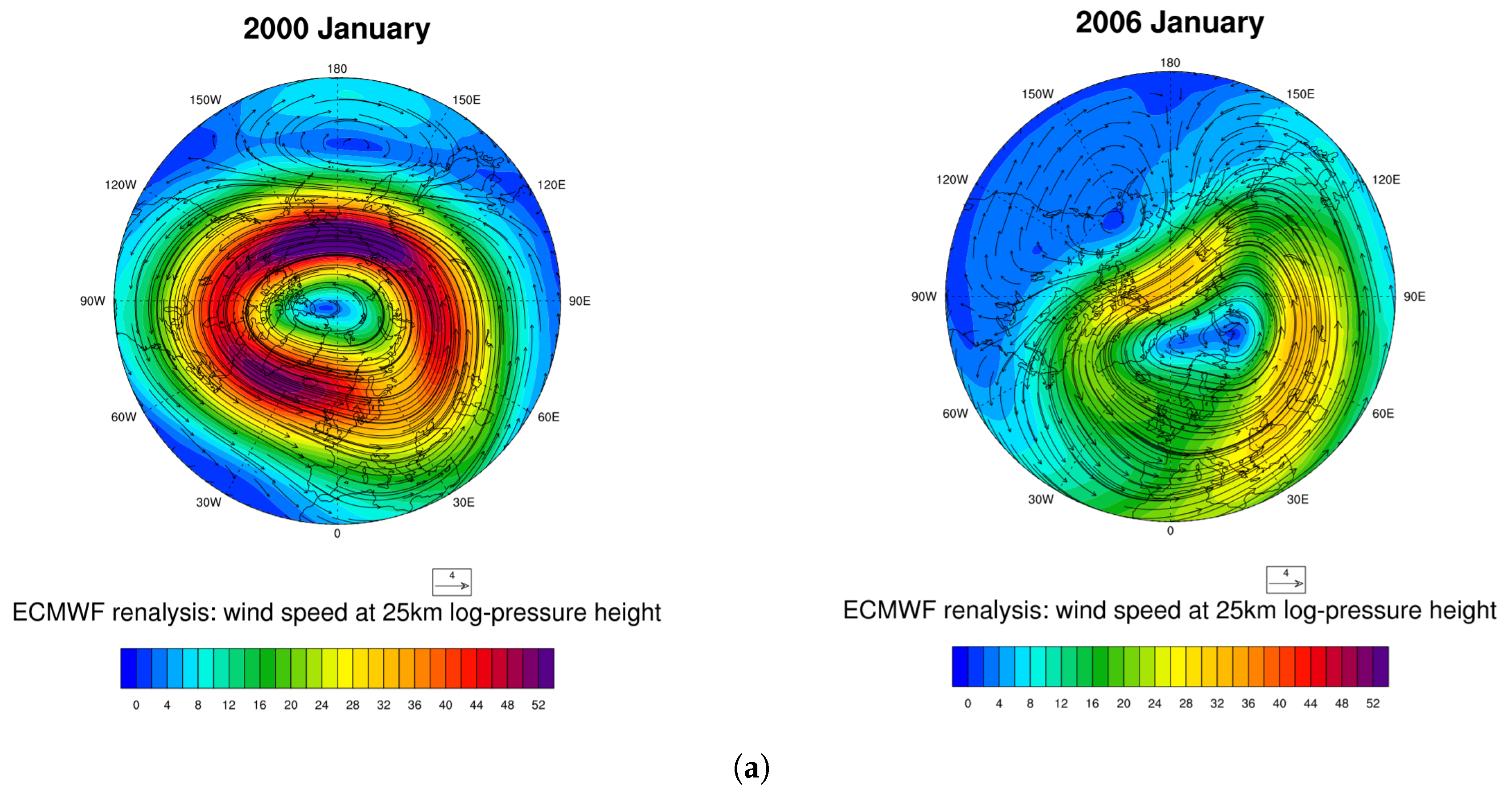
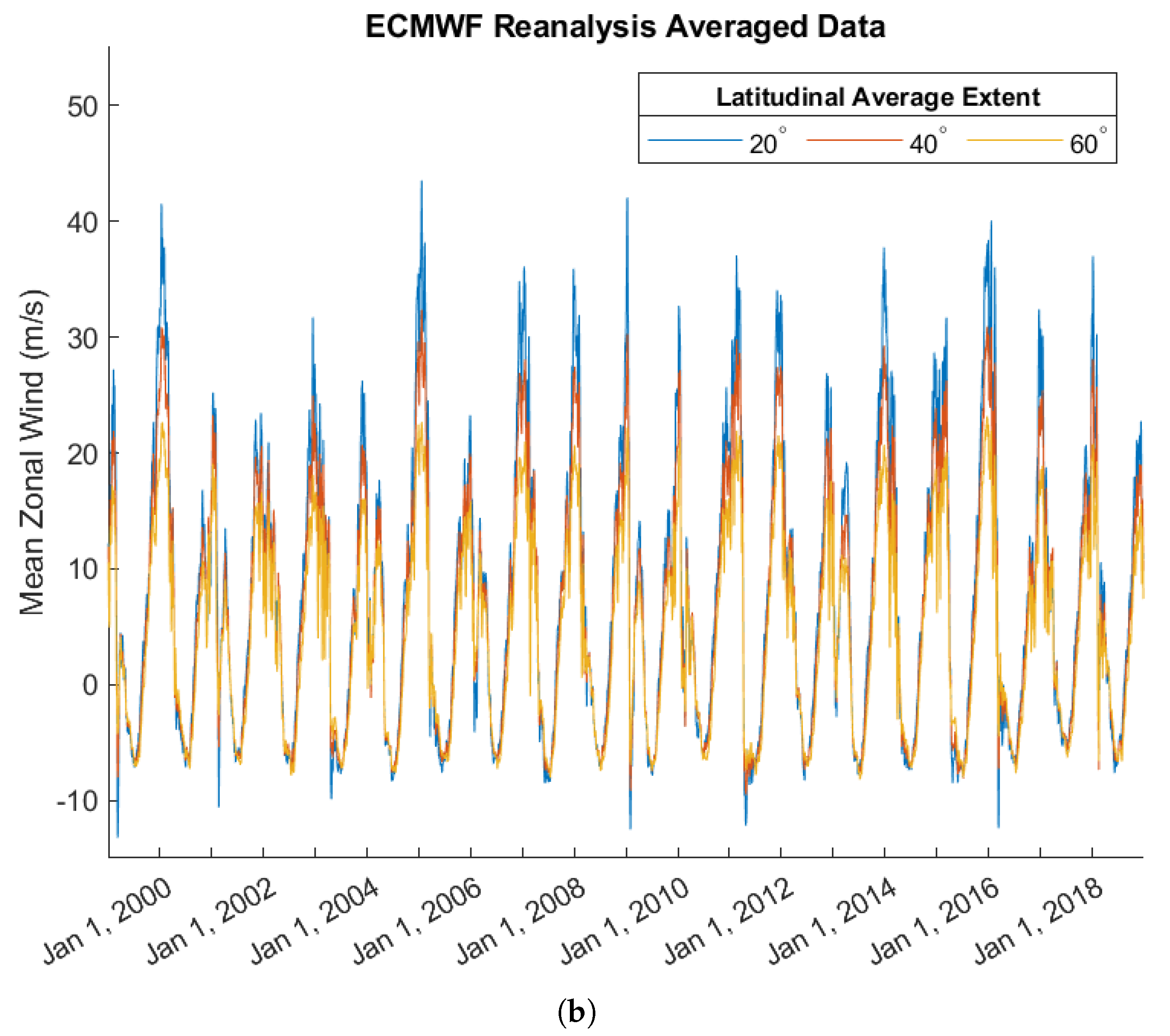
2.2. ECMWF Data
2.3. Data Assimilation
2.3.1. Particle Filter
2.3.2. ESMDA
- We start by sampling a large ensemble of realizations of the prior uncertain parameters, given their prescribed first-guess values and standard deviations;
- We then integrate the ensemble of model realizations forward in time to produce a prior ensemble prediction, which also characterizes the uncertainty;
- We compute the posterior ensemble of parameters by making use of the misfit between prediction and observations, and the correlations between the input parameters and the predicted measurements;
- Ultimately, we compute the posterior ensemble prediction by a forward ensemble integration. The posterior ensemble is then the “optimal” model prediction with the ensemble spread representing the uncertainty.
2.3.3. Twin Model Analysis
3. Results
3.1. Particle Filter
3.1.1. Identical Twin Model Experiments
3.1.2. ECMWF Data Assimilation
3.1.3. Particle Filter Summary
3.2. ESMDA Analysis
3.2.1. Free Parameters
3.2.2. Identical Twin Model Experiments
3.2.3. Parameterized and Free
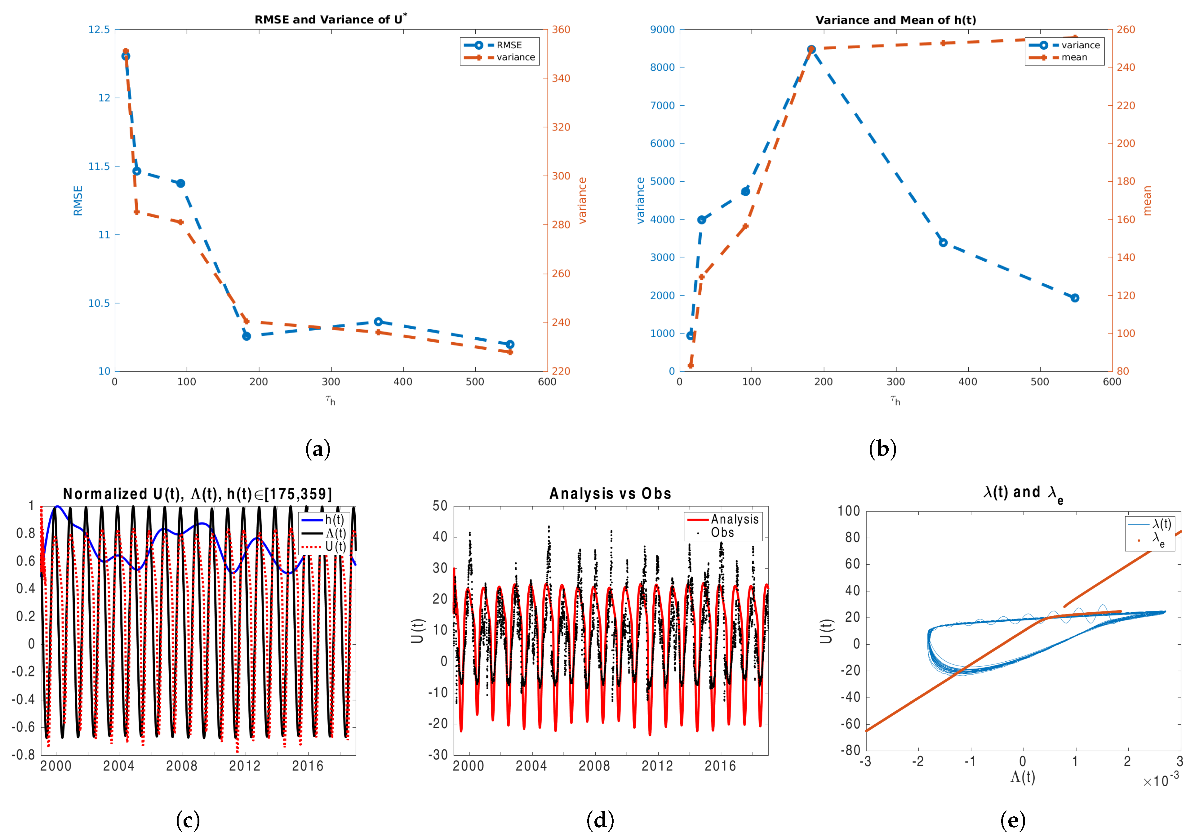
3.2.4. Free and Constant h
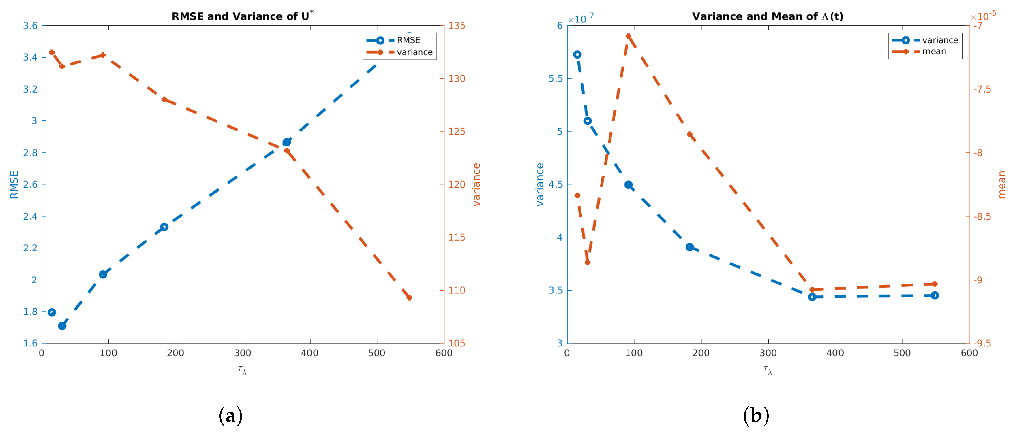
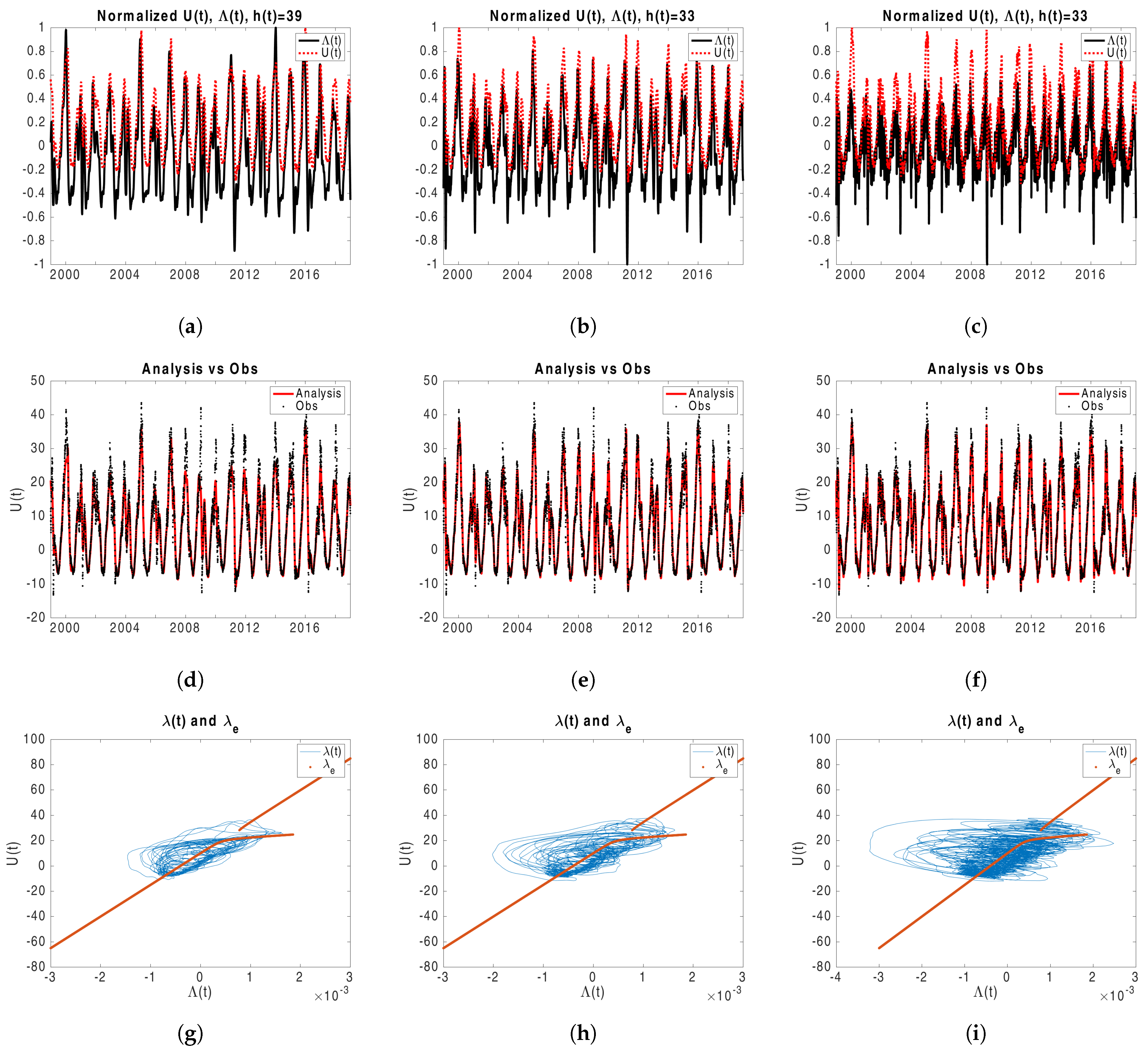
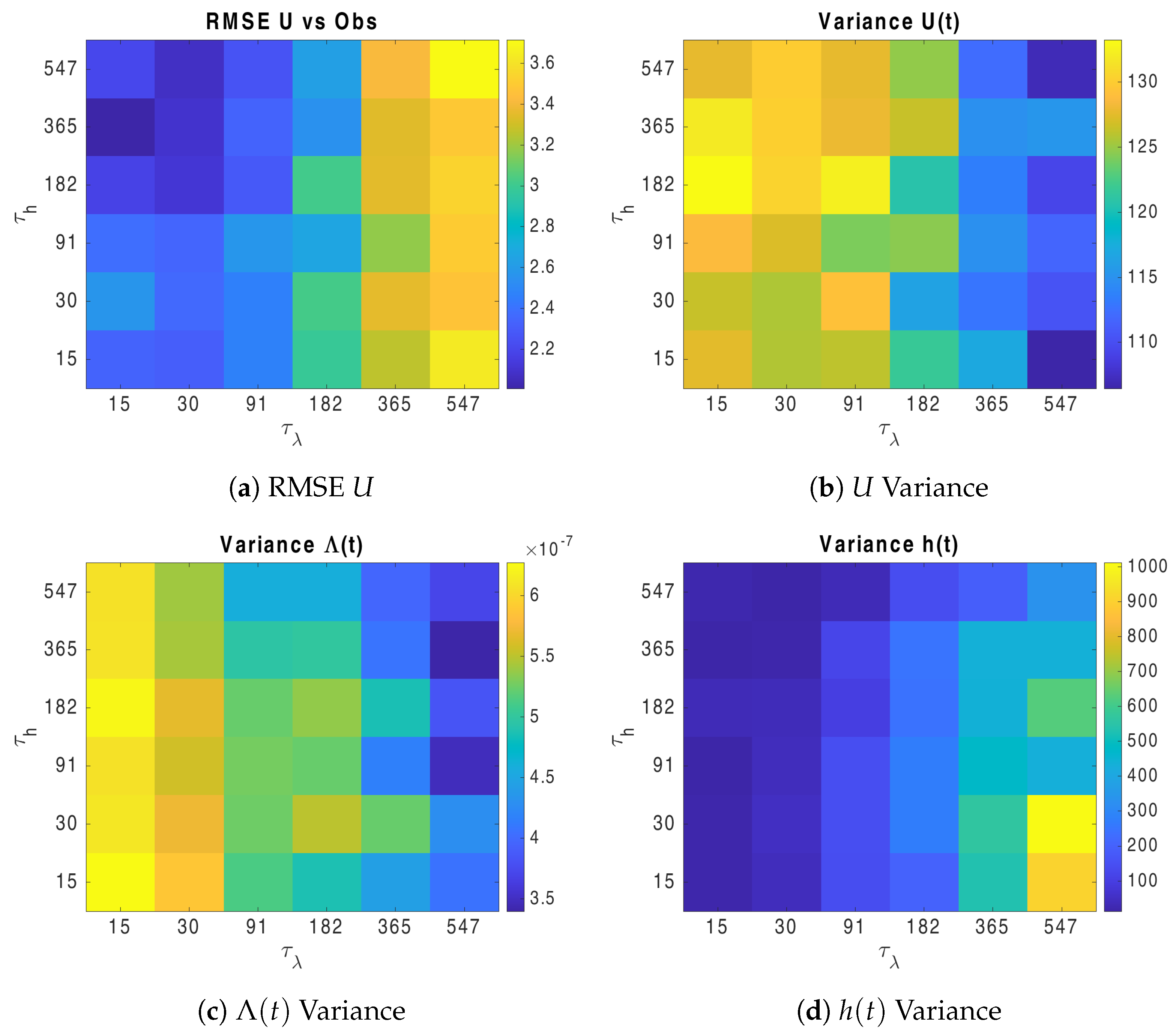
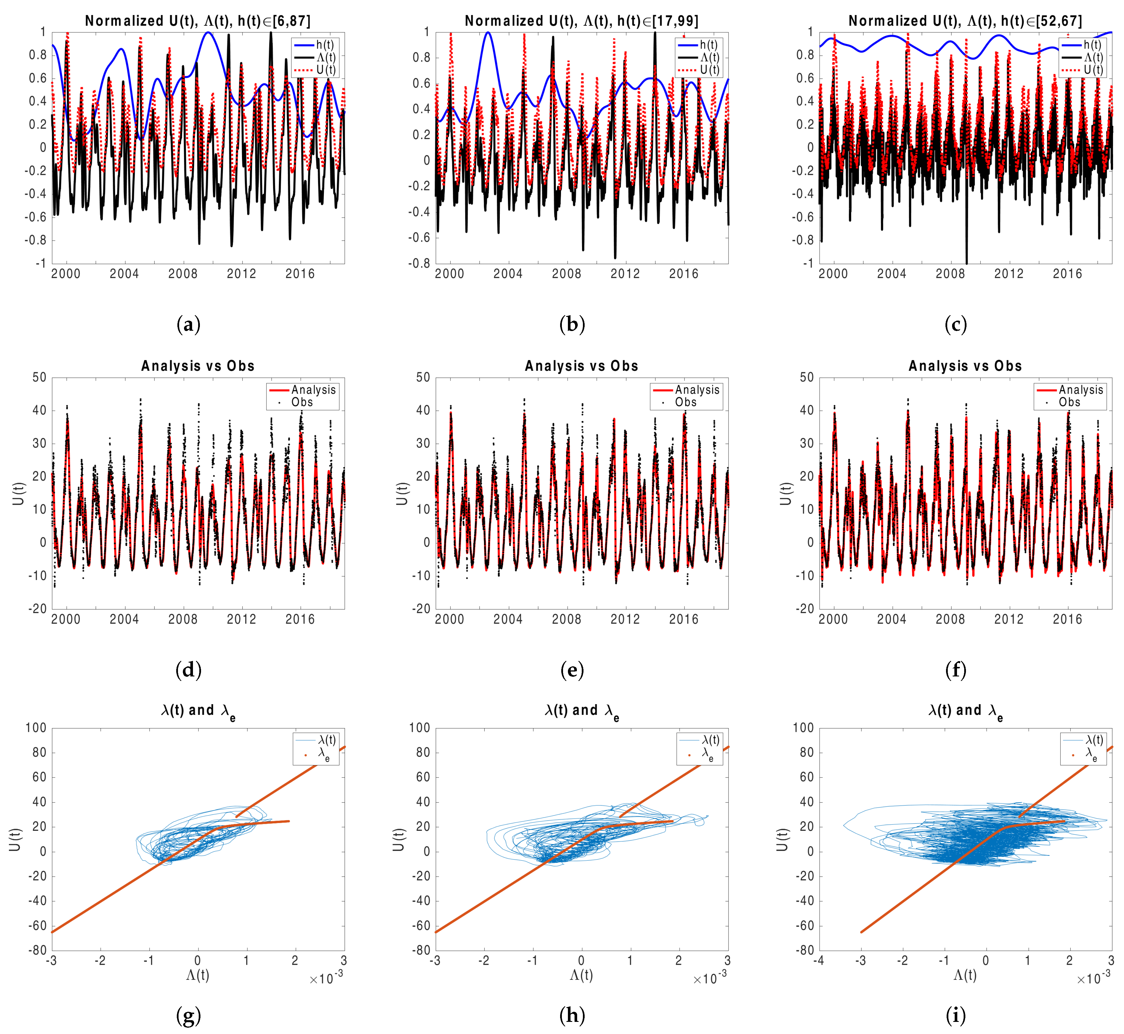
3.2.5. Free and
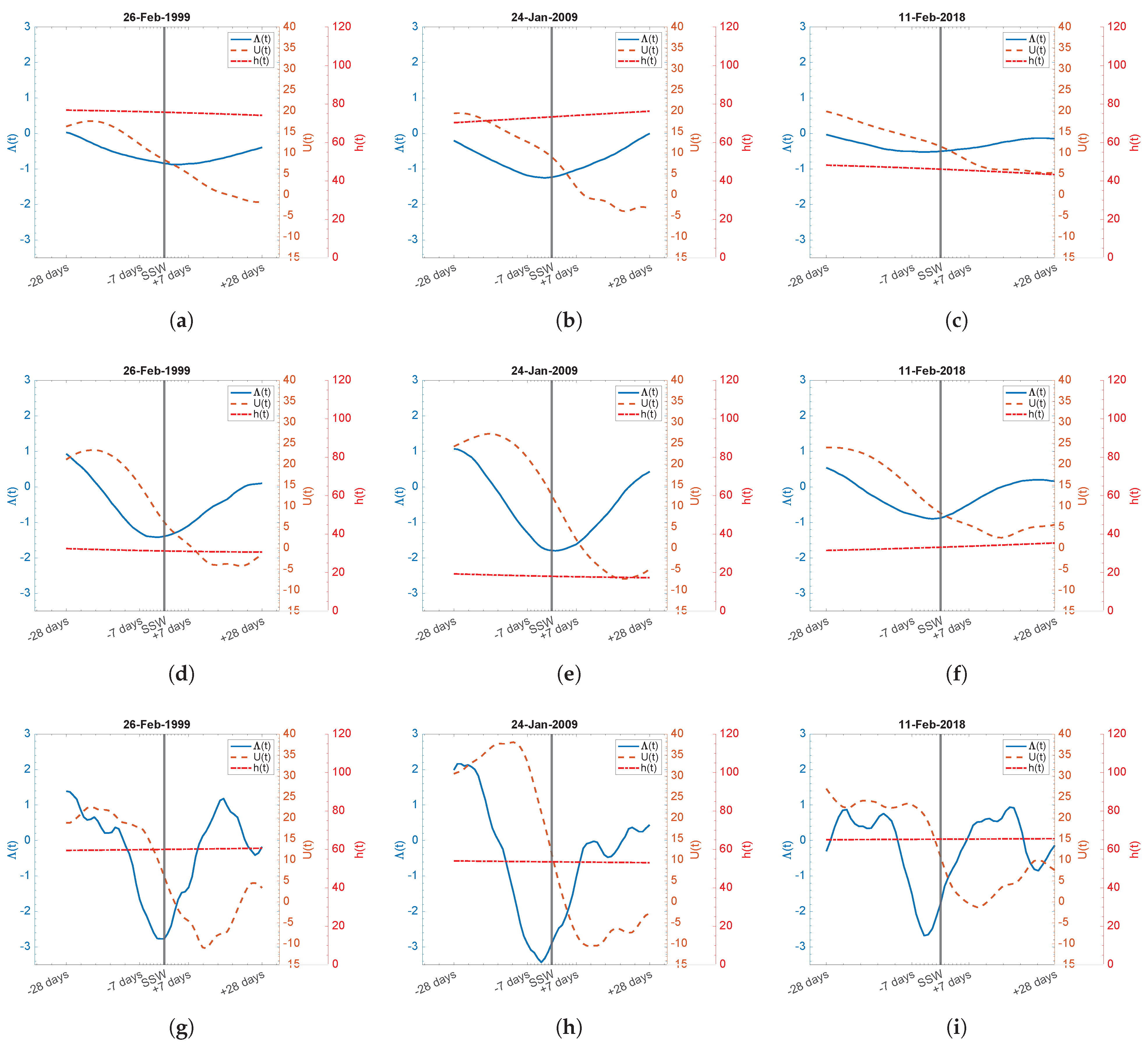
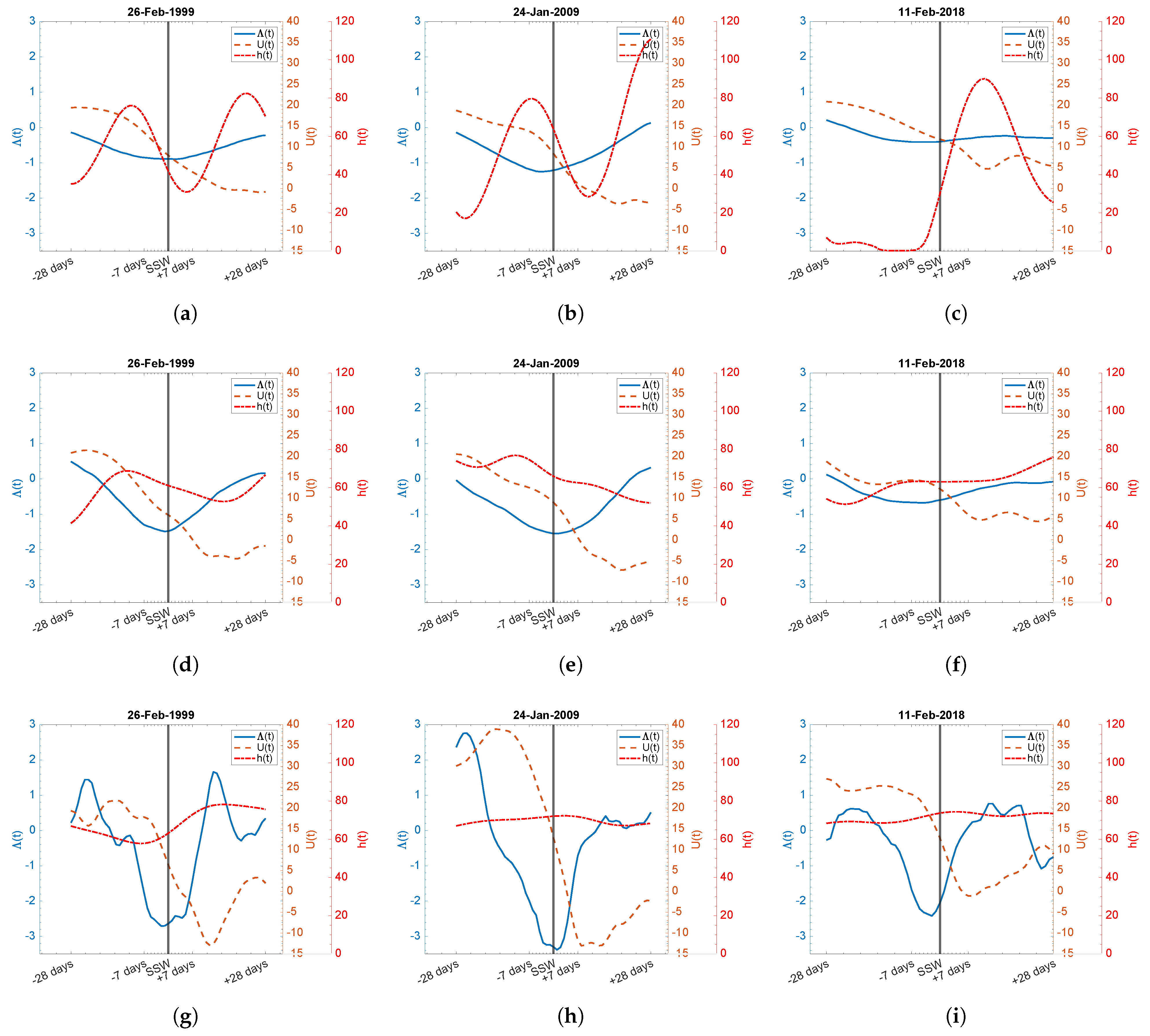
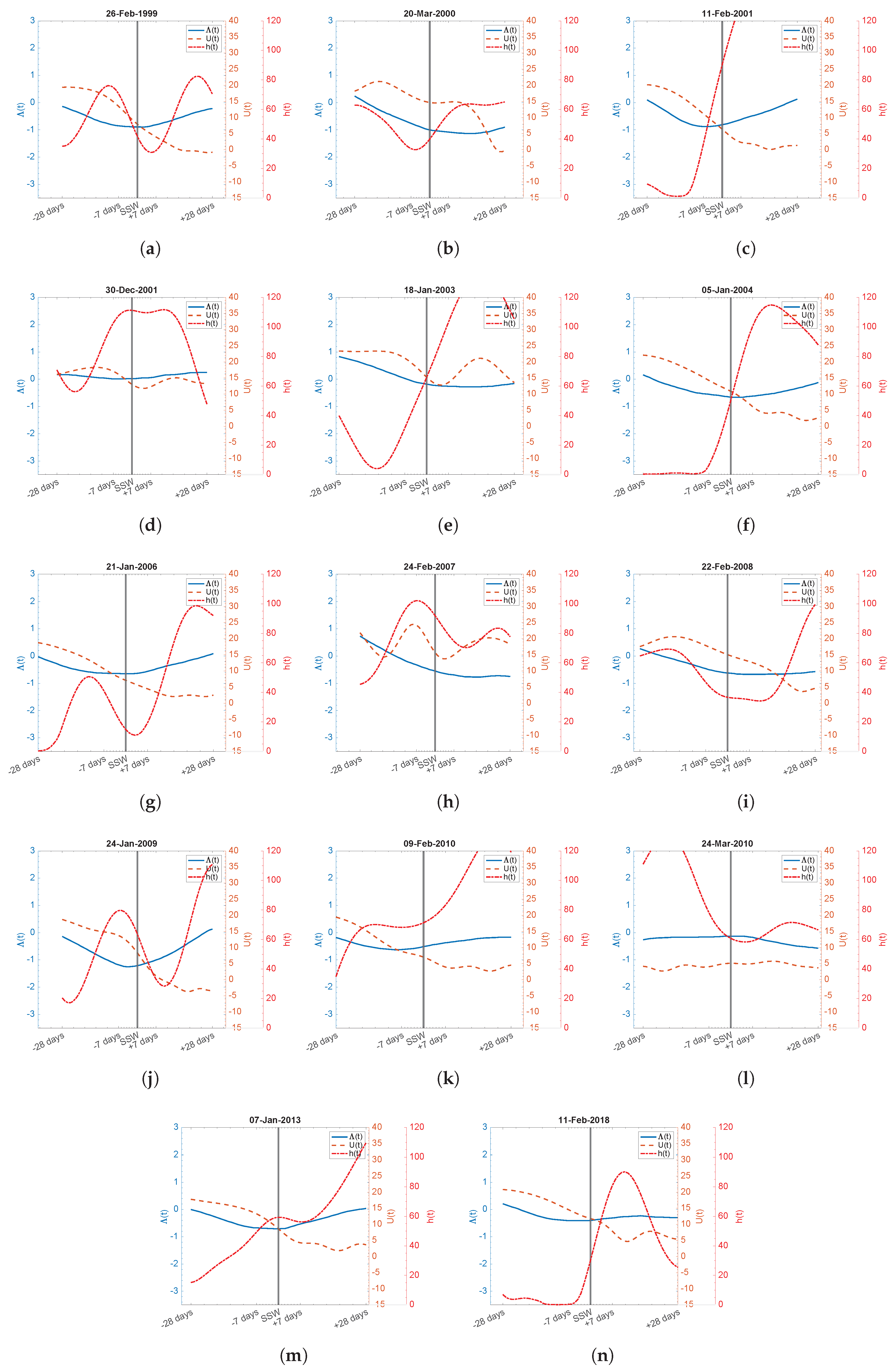
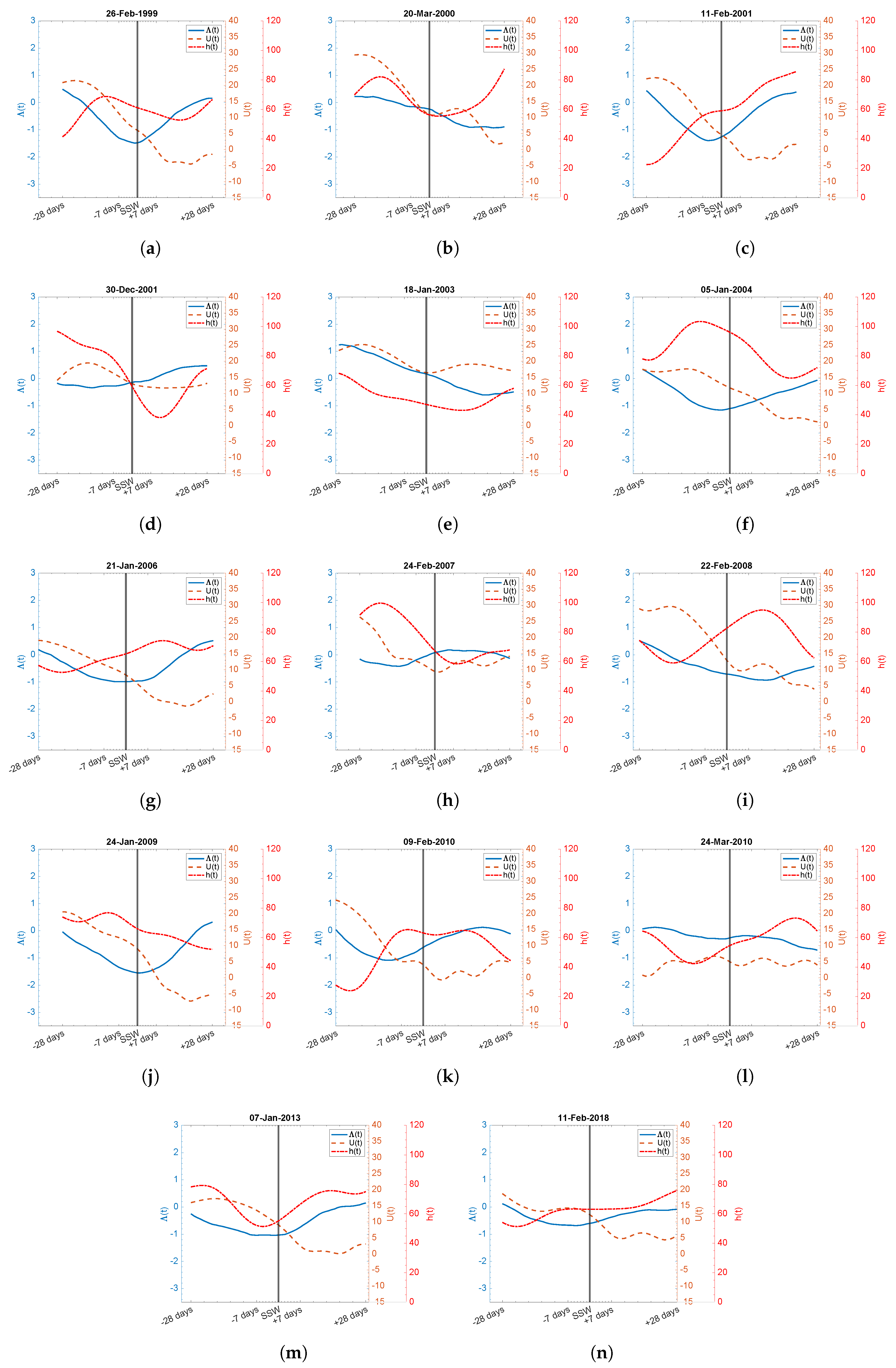
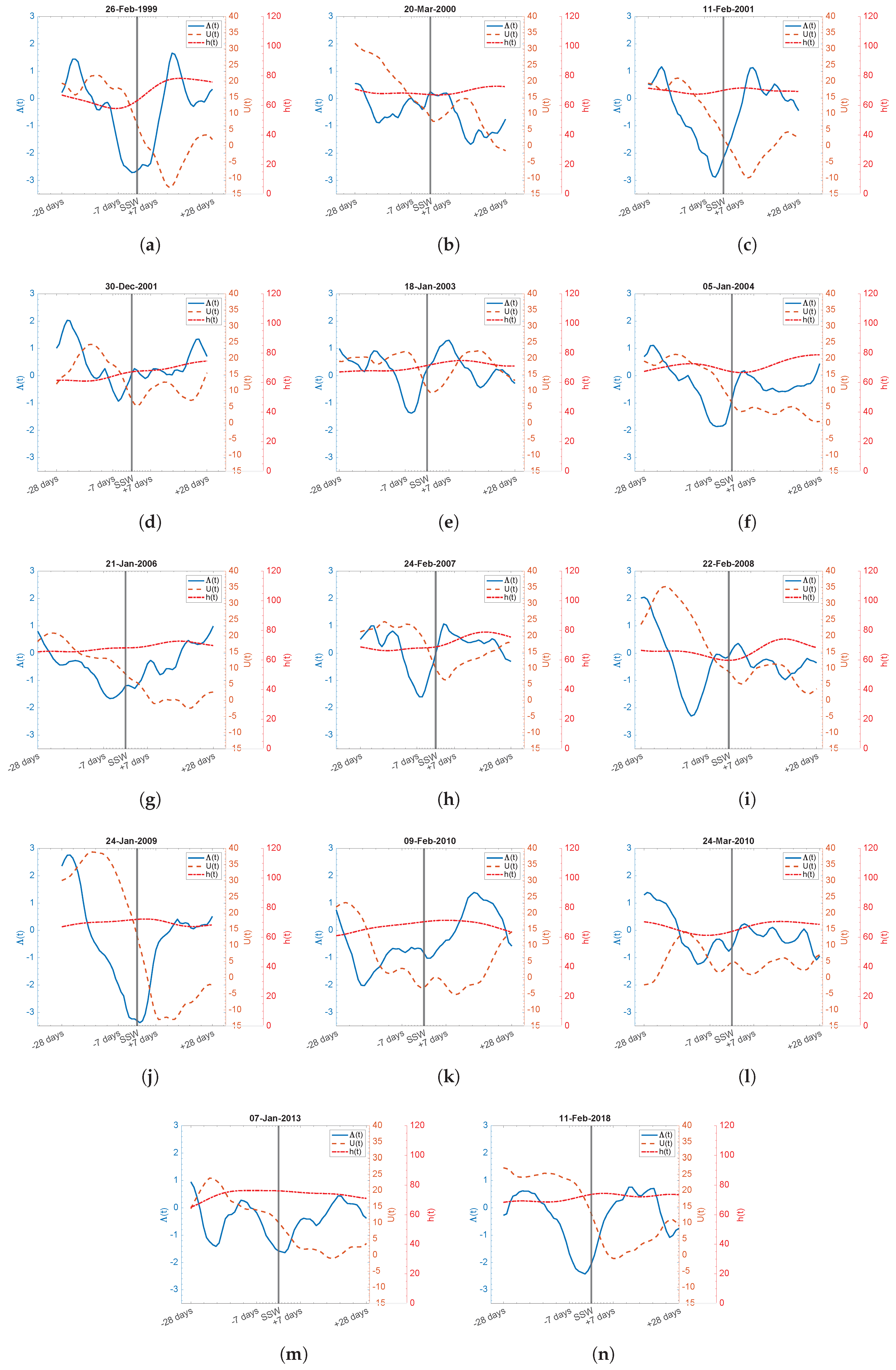
3.3. Analysis around SSW Events
4. Conclusions and Discussion
Author Contributions
Funding
Data Availability Statement
Acknowledgments
Conflicts of Interest
Appendix A

Appendix B
Appendix C


Appendix D


References
- Muench, H.S. On the dynamics of the wintertime stratosphere circulation. J. Atmos. Sci. 1965, 22, 349–360. [Google Scholar] [CrossRef]
- Geisler, J. A numerical model of the sudden stratospheric warming mechanism. J. Geophys. Res. 1974, 79, 4989–4999. [Google Scholar] [CrossRef]
- Charney, J.G.; DeVore, J.G. Multiple flow equilibria in the atmosphere and blocking. J. Atmos. Sci. 1979, 36, 1205–1216. [Google Scholar] [CrossRef]
- Ambaum, M.H.P.; Hoskins, B.J. The NAO Troposphere–Stratosphere Connection. J. Clim. 2002, 15, 1969–1978. [Google Scholar] [CrossRef]
- Finkel, J.; Abbot, D.S.; Weare, J. Path properties of atmospheric transitions: Illustration with a low-order sudden stratospheric warming model. J. Atmos. Sci. 2020, 77, 2327–2347. [Google Scholar] [CrossRef]
- Holton, J.R.; Mass, C. Stratospheric vacillation cycles. J. Atmos. Sci. 1976, 33, 2218–2225. [Google Scholar] [CrossRef]
- McIntyre, M.E. How well do we understand the dynamics of stratospheric warmings? J. Meteorol. Soc. Japan. Ser. II 1982, 60, 37–65. [Google Scholar] [CrossRef]
- Scott, R.; Polvani, L.M. Internal variability of the winter stratosphere. Part I: Time-independent forcing. J. Atmos. Sci. 2006, 63, 2758–2776. [Google Scholar] [CrossRef]
- Stan, C.; Straus, D.M. Stratospheric predictability and sudden stratospheric warming events. J. Geophys. Res. Atmos. 2009, 114. [Google Scholar] [CrossRef]
- Jeppesen, J. Fact Sheet: Reanalysis. 2020. Available online: https://www.ecmwf.int/en/about/media-centre/focus/2020/fact-sheet-reanalysis (accessed on 31 July 2021).
- Kantas, N.; Doucet, A.; Singh, S.S.; Maciejowski, J.; Chopin, N. On particle methods for parameter estimation in state-space models. Stat. Sci. 2015, 30, 328–351. [Google Scholar] [CrossRef]
- Gordon, N.J.; Salmond, D.J.; Smith, A.F. Novel approach to nonlinear/non-Gaussian Bayesian state estimation. In Proceedings of the IEE Proceedings F-Radar and Signal Processing; IET: Stevenage, UK, 1993; Volume 140, pp. 107–113. [Google Scholar]
- Asch, M.; Bocquet, M.; Nodet, M. Data Assimilation: Methods, Algorithms, and Applications; SIAM, Society for Industrial and Applied Mathematics: Philadelphia, PA, USA, 2016. [Google Scholar]
- Bocquet, M.; Sakov, P. An iterative ensemble Kalman smoother. Q. J. R. Meteorol. Soc. 2013, 140, 1521–1535. [Google Scholar] [CrossRef]
- Carrassi, A.; Bocquet, M.; Bertino, L.; Evensen, G. Data Assimilation in the Geosciences—An overview on methods, issues and perspectives. arXiv 2018, arXiv:1709.02798. [Google Scholar] [CrossRef]
- Skjervheim, J.; Evensen, G. An ensemble smoother for assisted history matching. In Proceedings of the SPE Reservoir Simulation Symposium, Woodlands, TX, USA, 21–23 February 2011; SPE 141929. SPE: Richardson, TX, USA, 2011. [Google Scholar] [CrossRef]
- Ruzmaikin, A.; Lawrence, J.; Cadavid, C. A simple model of stratospheric dynamics including solar variability. J. Clim. 2003, 16, 1593–1600. [Google Scholar] [CrossRef]
- Andrews, D.G.; Holton, J.R.; Leovy, C.B. Middle Atmosphere Dynamics; Number 40; Academic Press: Cambridge, MA, USA, 1987. [Google Scholar]
- Eichelberger, S.J.; Holton, J.R. A mechanistic model of the northern annular mode. J. Geophys. Res. Atmos. 2002, 107, ACL 10-1–ACL 10-12. [Google Scholar] [CrossRef]
- Wakata, Y.; Uryu, M. Stratospheric multiple equilibria and seasonal variations. J. Meteorol. Soc. Japan. Ser. II 1987, 65, 27–42. [Google Scholar] [CrossRef]
- Yoden, S. An illustrative model of seasonal and interannual variations of the stratospheric circulation. J. Atmos. Sci. 1990, 47, 1845–1853. [Google Scholar] [CrossRef]
- Sanchez, K. Understanding the Stratospheric Polar Vortex: A Parameter Sensitivity Analysis on a Simple Model of Stratospheric Dynamics. Ph.D. Thesis, Sam Houston State University, Huntsville, TX, USA, 2020. [Google Scholar]
- Berrisford, P.; Kållberg, P.; Kobayashi, S.; Dee, D.; Uppala, S.; Simmons, A.; Poli, P.; Sato, H. Atmospheric conservation properties in ERA-Interim. Q. J. R. Meteorol. Soc. 2011, 137, 1381–1399. [Google Scholar] [CrossRef]
- Wu, Z. Data Assimilation and Uncertainty Quantification with Reduced-order Models. Ph.D. Thesis, Arizona State University, Tempe, AZ, USA, 2021. [Google Scholar]
- Smith, A.F.; Gelfand, A.E. Bayesian statistics without tears: A sampling–resampling perspective. Am. Stat. 1992, 46, 84–88. [Google Scholar]
- Marín, D.A.A. Particle Filter Tutorial. 2012. Available online: https://www.mathworks.com/matlabcentral/fileexchange/35468-particle-filter-tutorial (accessed on 2 April 2021).
- Pfister, R.; Schwarz, K.A.; Janczyk, M.; Dale, R.; Freeman, J. Good things peak in pairs: A note on the bimodality coefficient. Front. Psychol. 2013, 4, 700. [Google Scholar] [CrossRef]
- Freeman, J.B.; Dale, R. Assessing bimodality to detect the presence of a dual cognitive process. Behav. Res. Methods 2013, 45, 83–97. [Google Scholar] [CrossRef]
- Emerick, A.A.; Reynolds, A.C. Ensemble smoother with multiple data assimilation. Comput. Geosci. 2013, 55, 3–15. [Google Scholar] [CrossRef]
- Fleurantin, E.; Sampson, C.; Maes, D.P.; Bennett, J.; Fernandes-Nunez, T.; Marx, S.; Evensen, G. A study of disproportionately affected populations by race/ethnicity during the SARS-CoV-2 pandemic using multi-population SEIR modeling and ensemble data assimilation. Found. Data Sci. 2021, 3, 479–541. [Google Scholar] [CrossRef]
- Evensen, G. EnKF_seir. 2021. Available online: https://github.com/geirev/EnKF_seir (accessed on 30 January 2021).
- Lawson, L.M.; Spitz, Y.H.; Hofmann, E.E.; Long, R.B. A data assimilation technique applied to a predator-prey model. Bull. Math. Biol. 1995, 57, 593–617. [Google Scholar] [CrossRef]
- Houtekamer, P.L.; Mitchell, H.L. Data assimilation using an ensemble Kalman filter technique. Mon. Weather Rev. 1998, 126, 796–811. [Google Scholar] [CrossRef]
- Browne, P.; Van Leeuwen, P. Twin experiments with the equivalent weights particle filter and HadCM3. Q. J. R. Meteorol. Soc. 2015, 141, 3399–3414. [Google Scholar] [CrossRef]
- Evensen, G. The Ensemble Kalman Filter: Theoretical formulation and practical implementation. Ocean Dyn. 2003, 53, 343–367. [Google Scholar] [CrossRef]
- Evensen, G. Sampling strategies and square root analysis schemes for the EnKF. Ocean Dyn. 2004, 54, 539–560. [Google Scholar] [CrossRef]
- Yoden, S. Bifurcation properties of a stratospheric vacillation model. J. Atmos. Sci. 1987, 44, 1723–1733. [Google Scholar] [CrossRef]
- Butler, A.H. Table of Major Mid-Winter SSWs in Reanalyses Products; NOAA Chemical Science Laboratory: Boulder, CO, USA, 2020. Available online: https://csl.noaa.gov/groups/csl8/sswcompendium/majorevents.html (accessed on 6 July 2023).
- Butler, A.H.; Seidel, D.J.; Hardiman, S.C.; Butchart, N.; Birner, T.; Match, A. Defining Sudden Stratospheric Warmings. Bull. Am. Meteorol. Soc. 2015, 96, 1913–1928. [Google Scholar] [CrossRef]
- Charlton, A.J.; Polvani, L.M. A New Look at Stratospheric Sudden Warmings. Part I: Climatology and Modeling Benchmarks. J. Clim. 2007, 20, 449–469. [Google Scholar] [CrossRef]
- Zuev, V.V.; Savelieva, E. Arctic polar vortex dynamics during winter 2006/2007. Polar Sci. 2020, 25, 100532. [Google Scholar] [CrossRef]
- Manabe, S.; Wetherald, R.T. Thermal Equilibrium of the Atmosphere with a Given Distribution of Relative Humidity. J. Atmos. Sci. 1967, 24, 241–259. [Google Scholar] [CrossRef]
- Santer, B.D.; Po-Chedley, S.; Zhao, L.; Zou, C.Z.; Fu, Q.; Solomon, S.; Thompson, D.W.J.; Mears, C.; Taylor, K.E. Exceptional stratospheric contribution to human fingerprints on atmospheric temperature. Proc. Natl. Acad. Sci. USA 2023, 120, e2300758120. [Google Scholar] [CrossRef]
- Holton, J.R.; Dunkerton, T. On the role of wave transience and dissipation in stratospheric mean flow vacillations. J. Atmos. Sci. 1978, 35, 740–744. [Google Scholar] [CrossRef]
- Keevil, J. ODE4 Gives More Accurate Results than ODE45, ODE23, ODE23s. 2016. Available online: https://www.mathworks.com/matlabcentral/fileexchange/59044-ode4-gives-more-accurate-results-than-ode45-ode23-ode23s (accessed on 13 May 2021).


Disclaimer/Publisher’s Note: The statements, opinions and data contained in all publications are solely those of the individual author(s) and contributor(s) and not of MDPI and/or the editor(s). MDPI and/or the editor(s) disclaim responsibility for any injury to people or property resulting from any ideas, methods, instructions or products referred to in the content. |
© 2023 by the authors. Licensee MDPI, Basel, Switzerland. This article is an open access article distributed under the terms and conditions of the Creative Commons Attribution (CC BY) license (https://creativecommons.org/licenses/by/4.0/).
Share and Cite
Sherman, J.; Sampson, C.; Fleurantin, E.; Wu, Z.; Jones, C.K.R.T. A Data-Driven Study of the Drivers of Stratospheric Circulation via Reduced Order Modeling and Data Assimilation. Meteorology 2024, 3, 1-35. https://doi.org/10.3390/meteorology3010001
Sherman J, Sampson C, Fleurantin E, Wu Z, Jones CKRT. A Data-Driven Study of the Drivers of Stratospheric Circulation via Reduced Order Modeling and Data Assimilation. Meteorology. 2024; 3(1):1-35. https://doi.org/10.3390/meteorology3010001
Chicago/Turabian StyleSherman, Julie, Christian Sampson, Emmanuel Fleurantin, Zhimin Wu, and Christopher K. R. T. Jones. 2024. "A Data-Driven Study of the Drivers of Stratospheric Circulation via Reduced Order Modeling and Data Assimilation" Meteorology 3, no. 1: 1-35. https://doi.org/10.3390/meteorology3010001