

System for Analysis of Wind Collocations (SAWC): A Novel Archive and Collocation Software Application for the Intercomparison of Winds from Multiple Observing Platforms

 , , , , and
Abstract
:1. Introduction
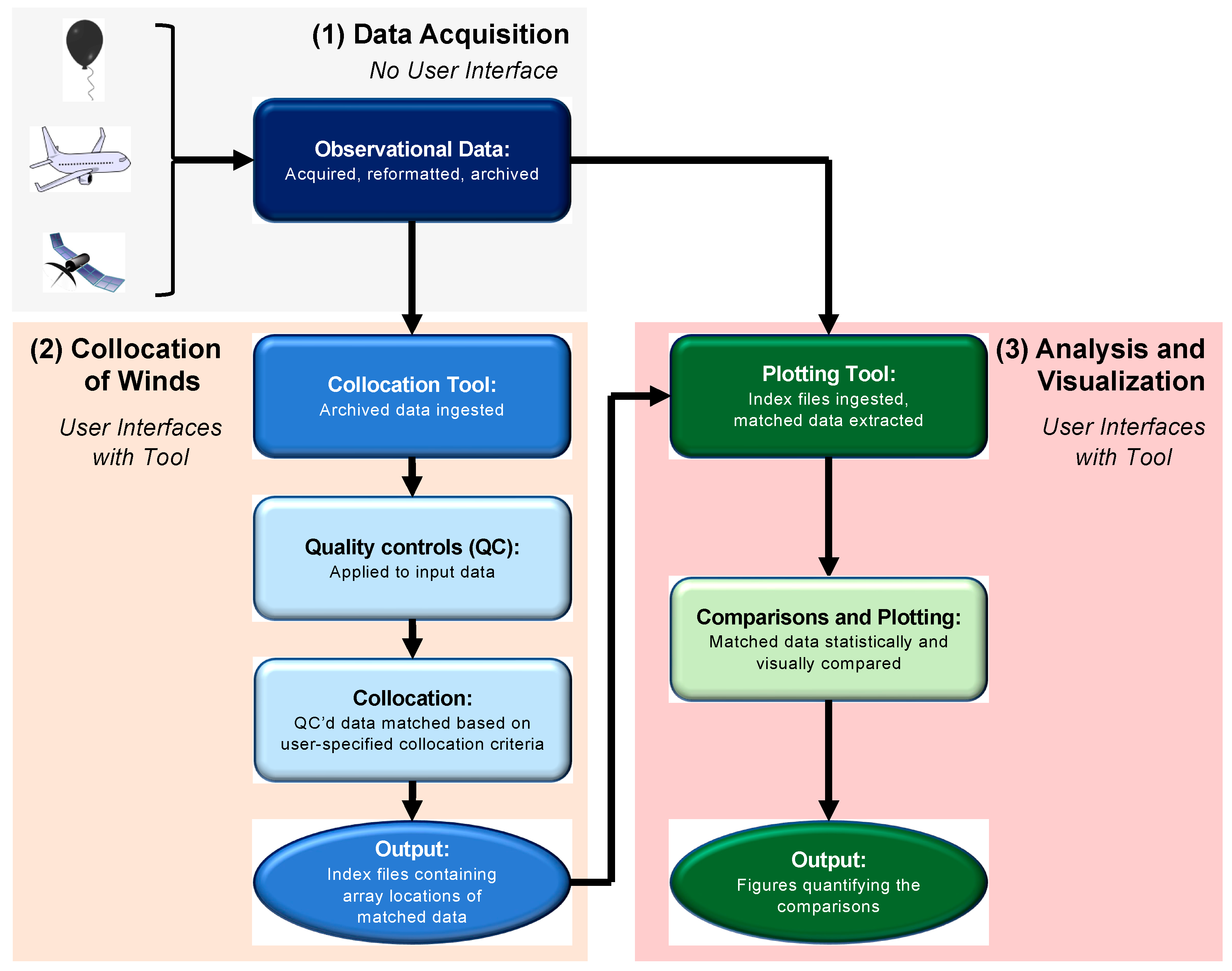
2. Overview of SAWC
- SAWC Website: https://www.star.nesdis.noaa.gov/sawc (accessed on 28 February 2024).
- Data Home: https://www.star.nesdis.noaa.gov/data/sawc (accessed on 28 February 2024).
- Wind Archive: https://www.star.nesdis.noaa.gov/data/sawc/wind_datasets (accessed on 28 February 2024).
- Collocation Software Application and Index Files: https://www.star.nesdis.noaa.gov/data/sawc/collocation (accessed on 28 February 2024).
- User Manual: https://www.star.nesdis.noaa.gov/data/sawc/User_Manual (accessed on 28 February 2024).
2.1. Datasets Available
2.2. Collocation Software Application
2.2.1. Collocation Tool
- Aeolus winds must be at pressures less than 800 hPa. Thus, all Aeolus boundary layer winds are rejected.
- Aeolus winds and AMVs must be high quality, as estimated by the data producers. For Aeolus, the L2B uncertainty must be small. For AMVs, the quality indicator (QI) must be at least 80.
2.2.2. Plotting Tool
3. Demonstrations of SAWC’s Utility
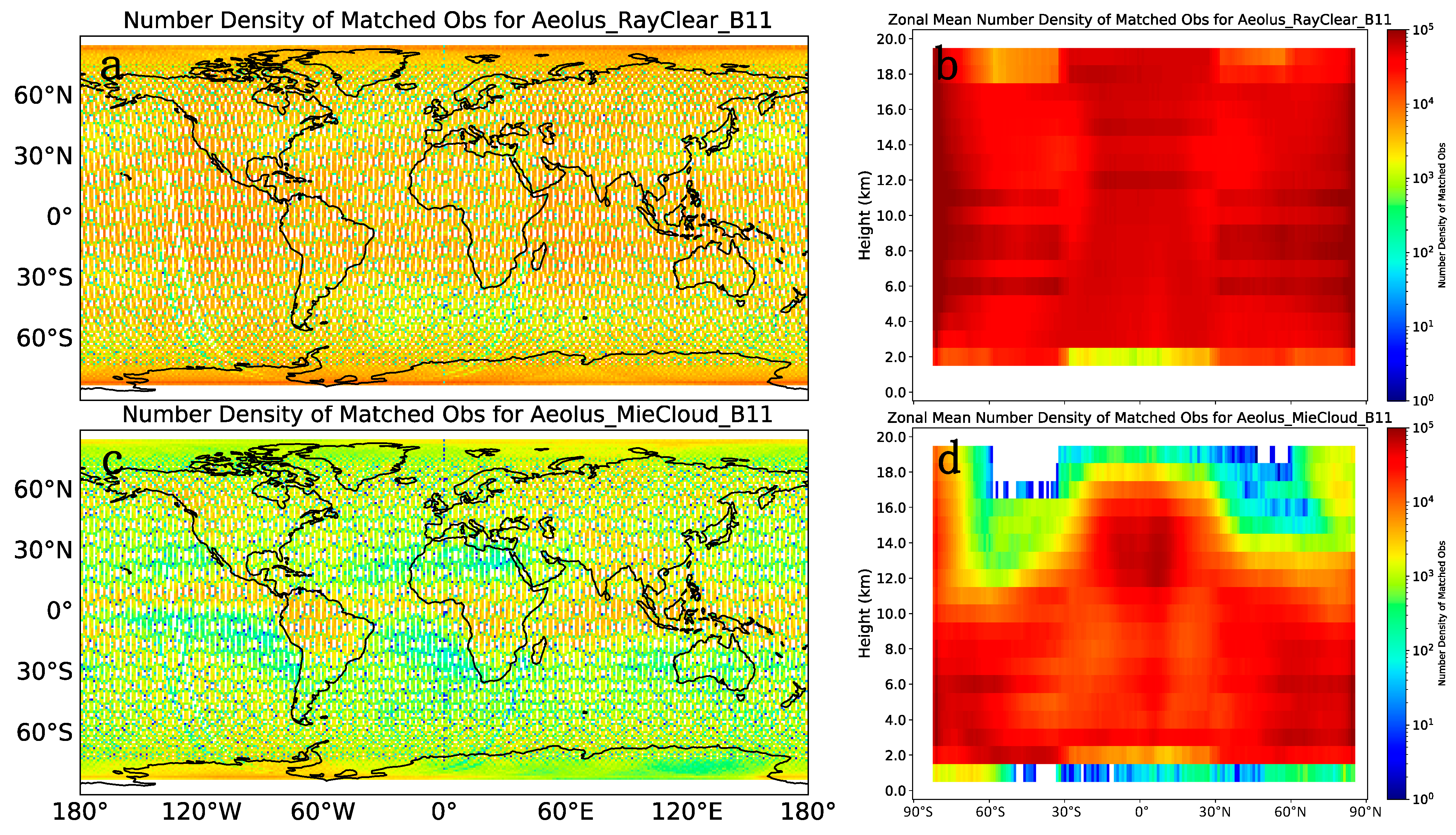
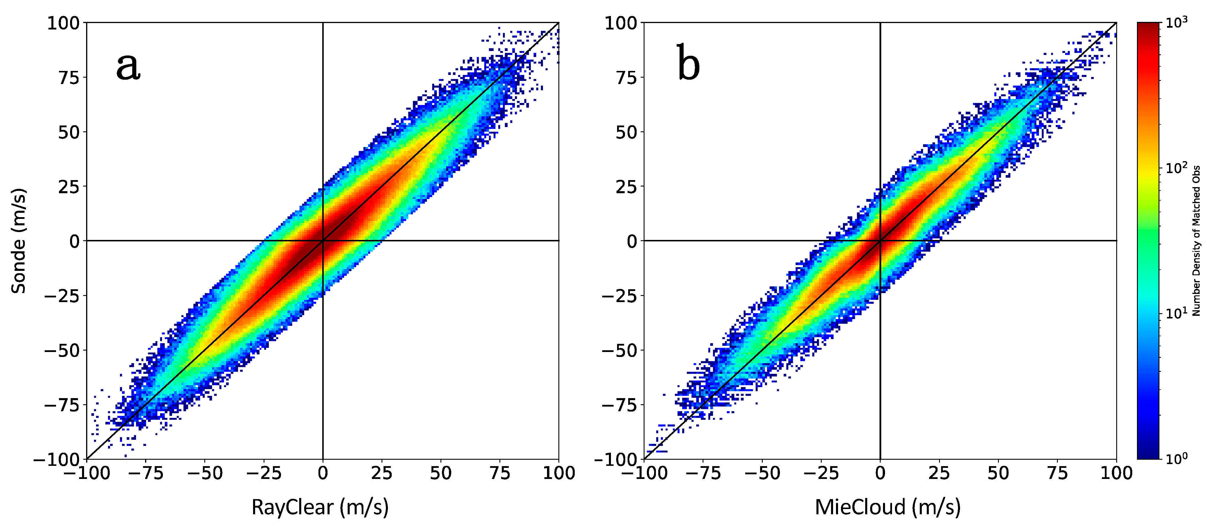
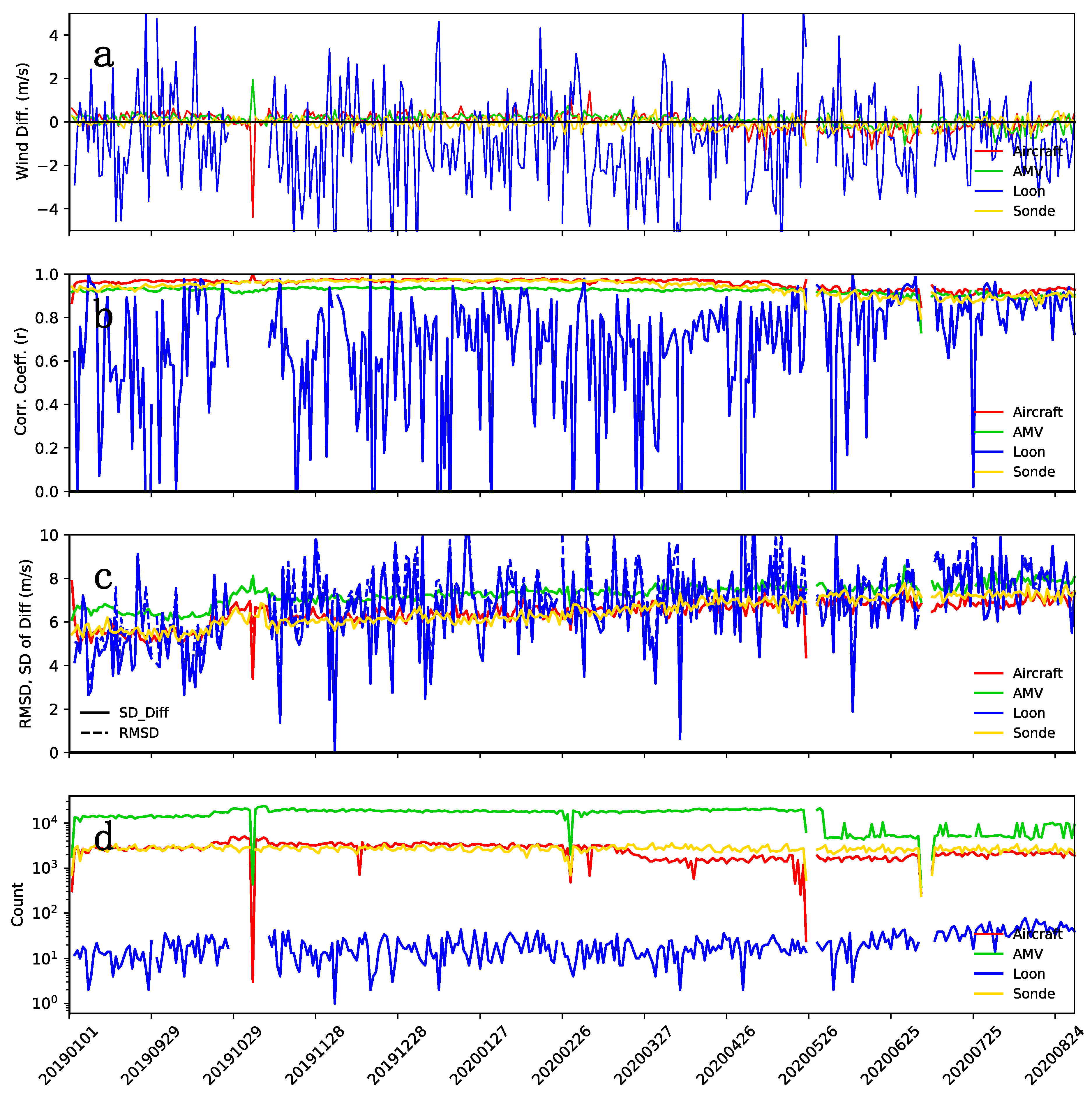
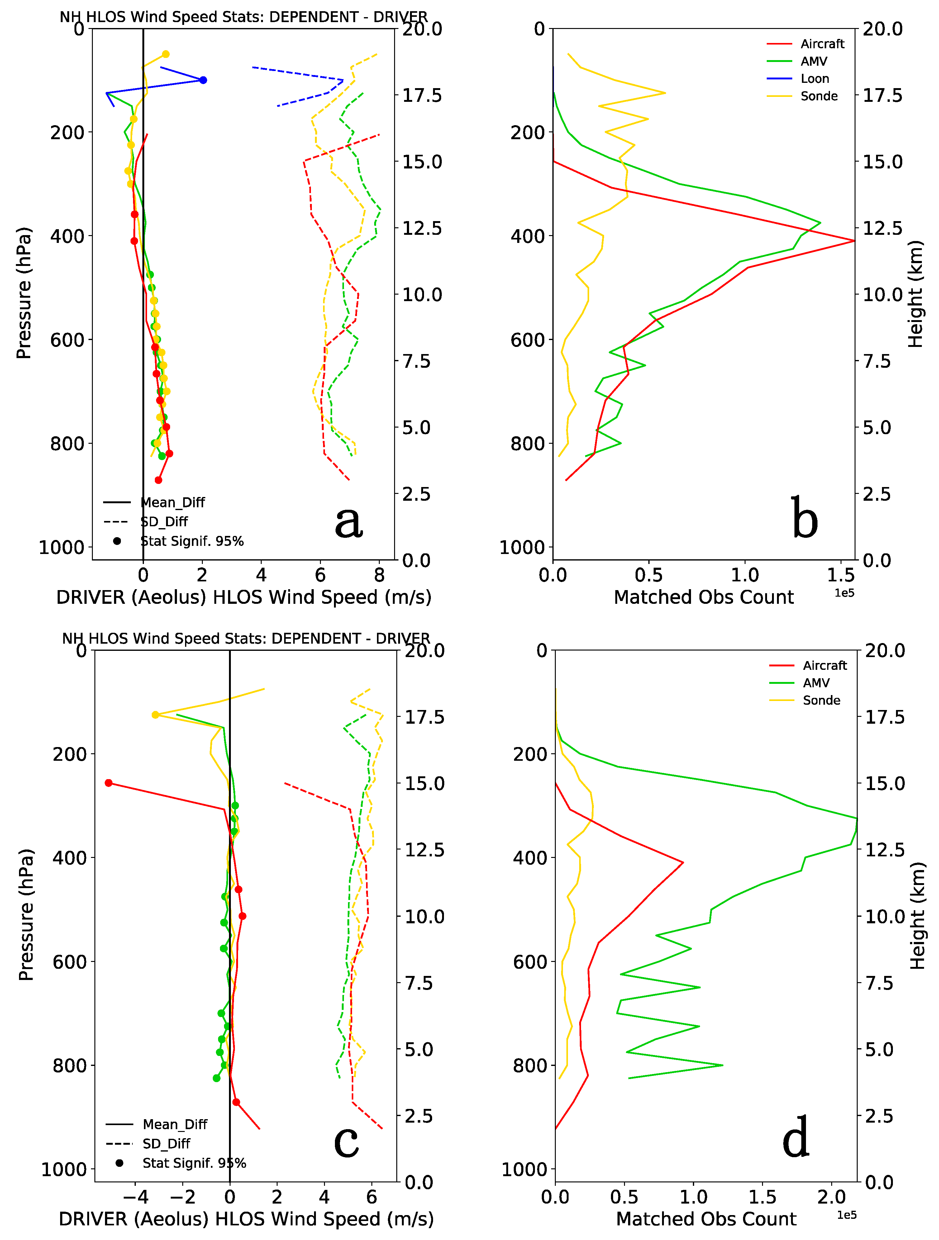
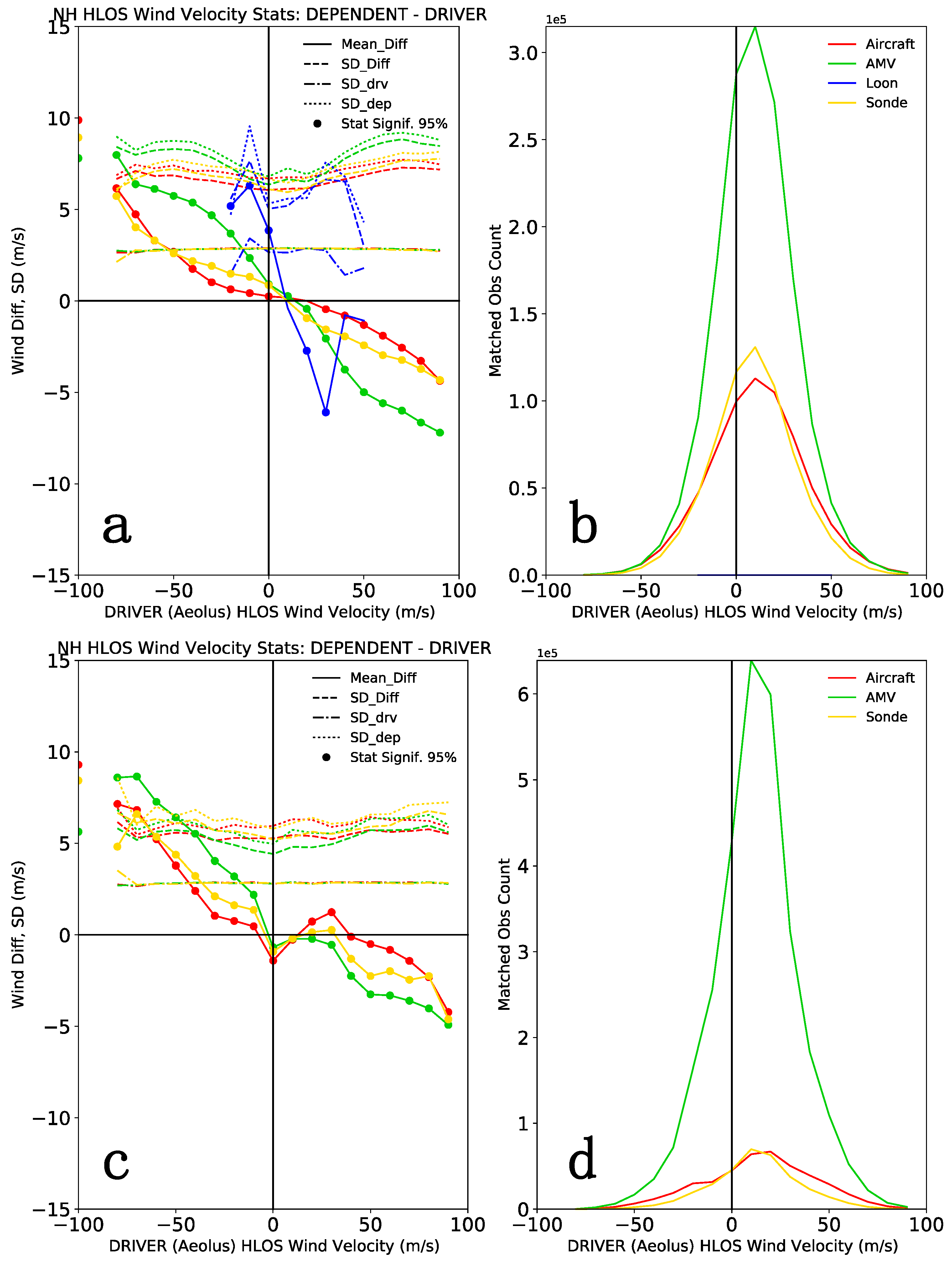
3.1. Comparisons between Wind Datasets
3.1.1. Dataset Comparison Results
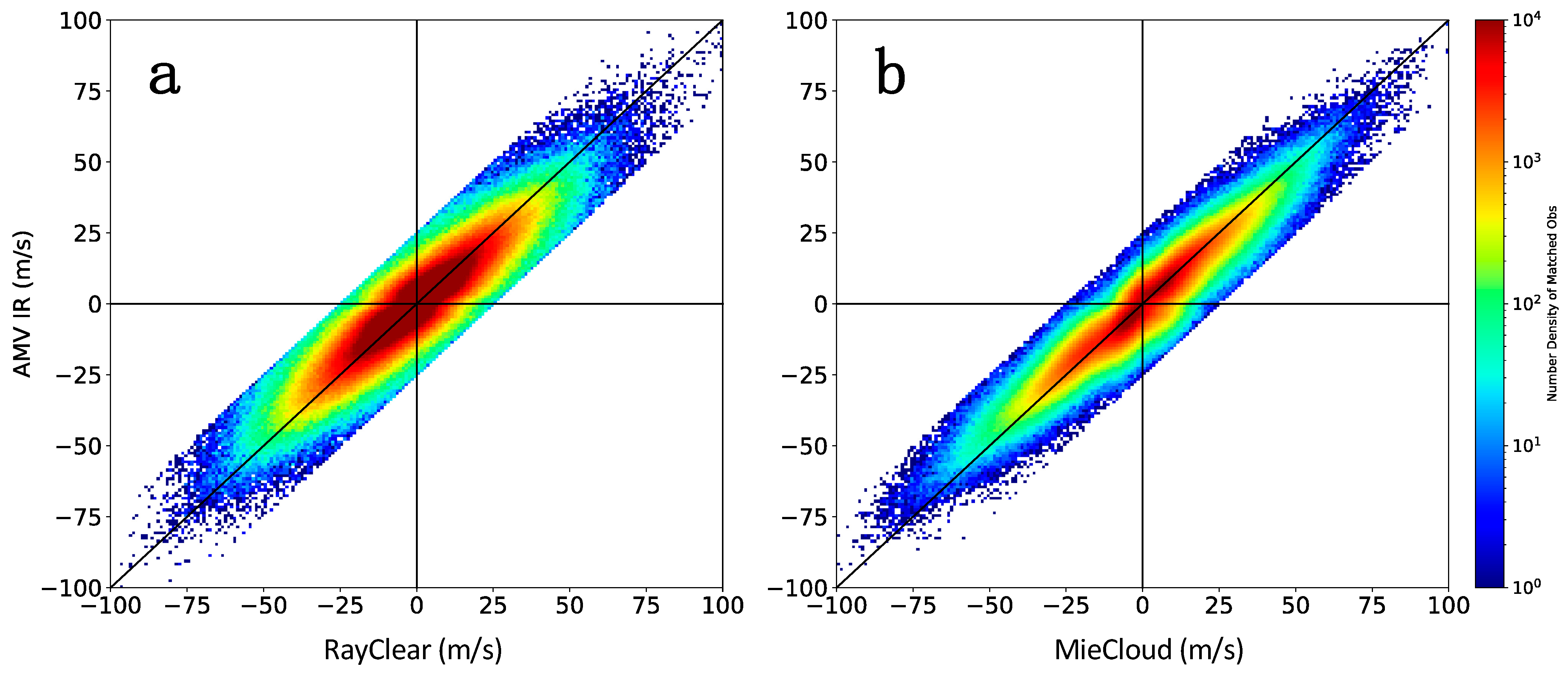
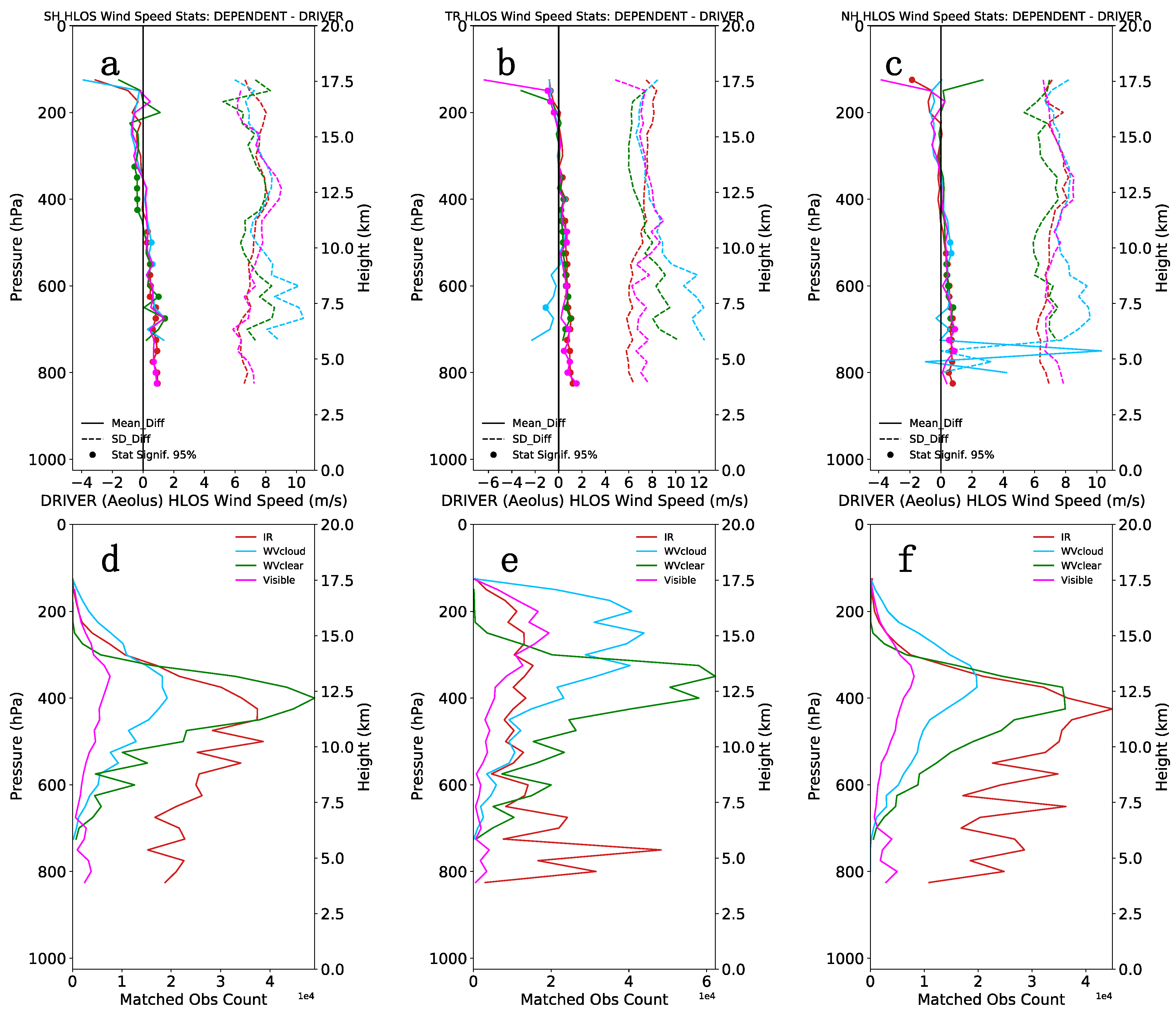
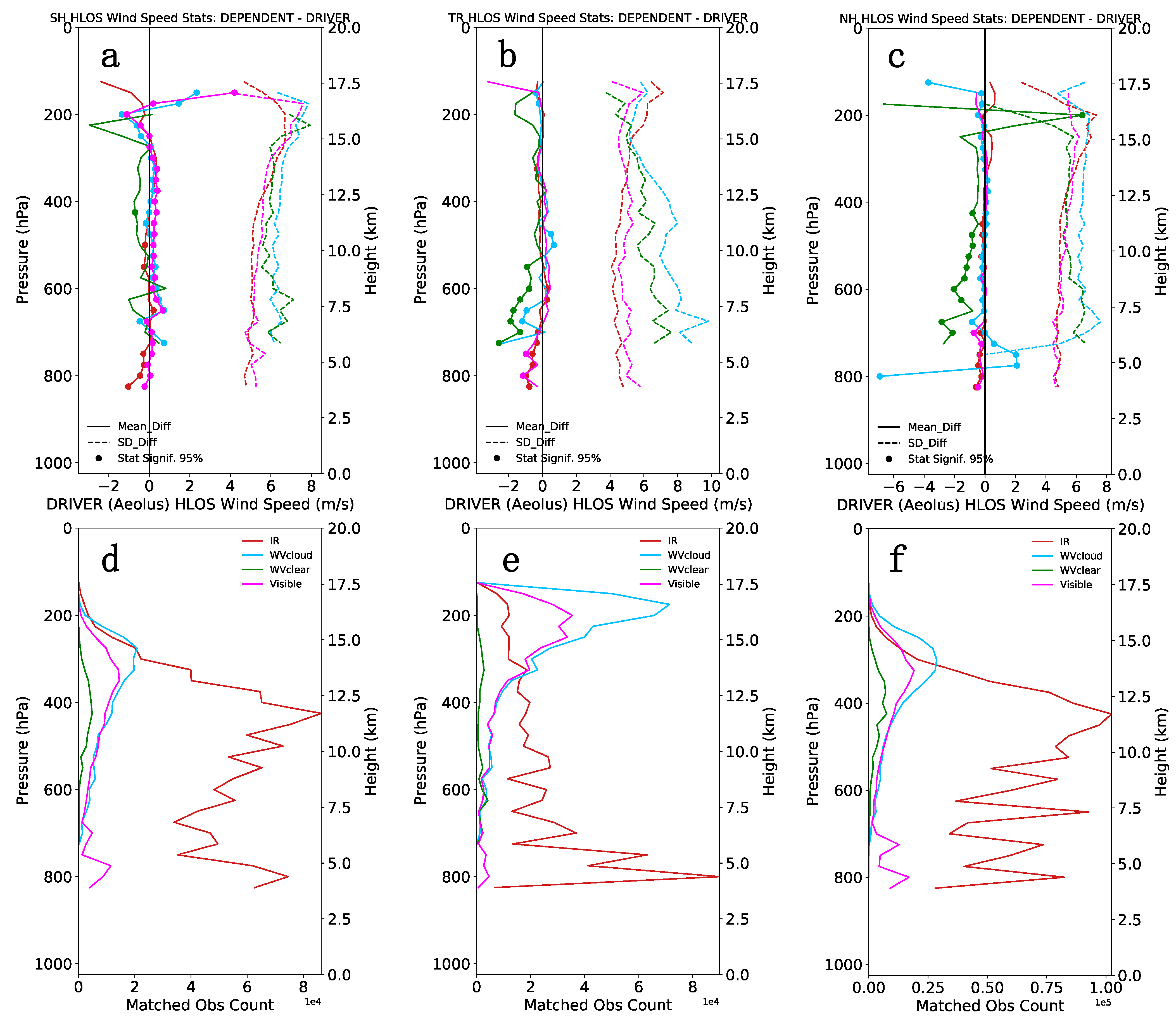
3.1.2. AMV Wind Types vs. Aeolus
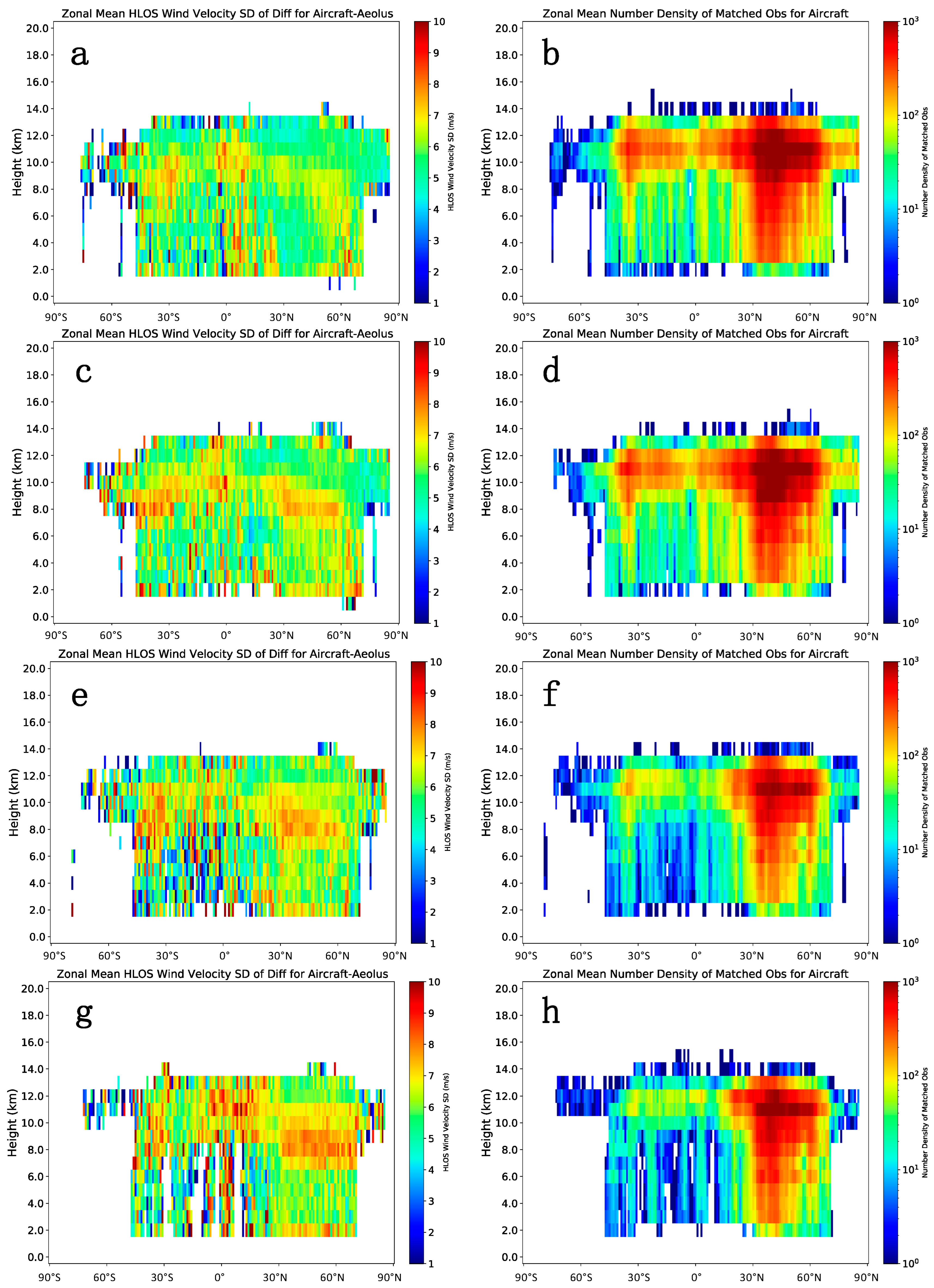
3.1.3. Aircraft vs. Aeolus during the COVID-19 Pandemic
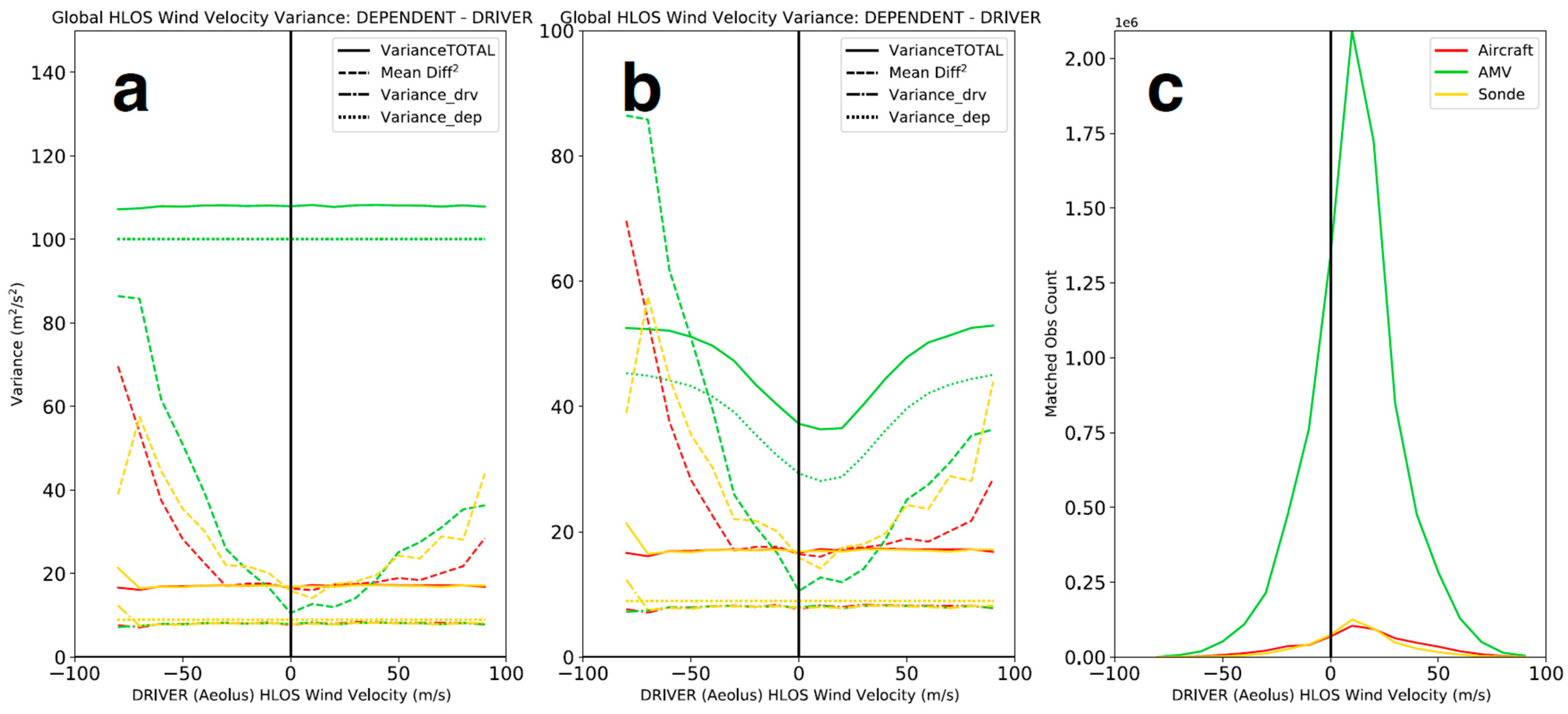
3.2. Observation Error Estimation for Data Assimilation
4. Summary and Discussion
- Data Acquisition, where wind observations are acquired from aircraft, satellites (Aeolus winds and AMVs), sondes, and stratospheric superpressure balloons (Figure S1); converted to a common format (netCDF); and archived.
- Collocation of Winds, where users can utilize the SAWC collocation tool developed for their intercomparison to produce a collection of matched winds between different datasets.
- Analysis and Visualization, where users can interact with the SAWC plotting tool to visually and statistically compare the matched winds based on their research needs.
Supplementary Materials
Author Contributions
Funding
Data Availability Statement
Acknowledgments
Conflicts of Interest
Appendix A

| SAWC Component | Formats | Temporal Coverage | Key Variables Available |
|---|---|---|---|
| Index Files | NetCDF-4 files | Select periods | Indices of matched winds; Differences in time, height/pressure, and distance for each pair of matched winds |
| Collocation Application | One tarball per application version, each containing Bash and Python scripts | N/A | N/A |
| Collocation Tool Parameter | Description |
|---|---|
| Date Range | Year, month, and range of days over which to run the collocation tool. |
| Dataset Names | Names of datasets to be collocated. (The first dataset listed is the Driver; all others are Dependents) |
| Path to Output Index Files | Full path to location where output collocation index files are to be saved. |
| Collocation Criteria | Four criteria: Max collocation distance in km; Max time difference in minutes; Max log10 (pressure) difference log10 (hPa); Max height difference in km. (Must have four criteria per Dependent dataset to be collocated) |
| Quality Control Flags | Quality control (QC) flags for each dataset (Driver and Dependents) indicating whether or not QC will be applied. Options: 0 (no QC applied); 1 (QC applied) |
| Number of Matches Allowed | Number of Dependent observations allowed to match each Driver observation. Default = 50 |
| AMV Quality Indicator | Quality indicator (QI) value in % for AMV observations. |
| AMV Quality Indicator Option | QI options for AMVs: Use QI variable without the forecast (NO_FC default); Use QI variable with the forecast (YES_FC) |
| Aeolus Dataset Type | Abbreviation for Aeolus L2B dataset type. Options: orig (dataset processed with original L2B processor at time of retrieval); B## (dataset reprocessed with a different L2B processor than that used at time of retrieval, where ## is a 2-digit number indicating the Baseline number, e.g., B10 = Baseline 10) |
| Dataset | QC Parameters |
|---|---|
| Aeolus Mie-cloudy | p > 800 hPa; σ > 5 m/s |
| Aeolus Rayleigh-clear | p > 800 hPa; σ > 8.5 m/s for 800 ≥ p > 200 hPa; σ > 12 m/s for p ≤ 200 hPa; z < 0.3 km; length < 60 km |
| AMV | QI < 80 |
| Dataset | Δt | Δx | Δp | Δz |
|---|---|---|---|---|
| Aeolus | 60 min | 100 km | 0.04 log10 (hPa) | 1 km |
| Aircraft | 60 min | 100 km | 0.04 log10 (hPa) | 1 km |
| AMV | 60 min | 100 km | 0.04 log10 (hPa) | 1 km |
| Loon | 60 min | 100 km | 0.04 log10 (hPa) | 1 km |
| Sonde | 90 min | 150 km | 0.04 log10 (hPa) | 1 km |
| Parameter | Description |
|---|---|
| Start Date, End Date | Start date and end date (year, month, day, hour) over which to run the collocation tool. |
| Driver Dataset Name | Name of Driver dataset. |
| Dependent Dataset Names | Names of Dependent datasets to be compared to the Driver. |
| Path to Input Index Files | Full path to location where input collocation index files are located. |
| Path to Output Plots | Full path to location where output plots are to be saved. |
| Super-ob Choice | Choice to super-ob (average) multiple collocations per Driver observation or use all collocations for statistical analysis. Options: −1 (use all collocations) or 0 (super-ob). |
Appendix B
References
- National Academies of Sciences, Engineering, and Medicine. Thriving on Our Changing Planet: A Decadal Strategy for Earth Observation from Space; National Academies Press: Washington, DC, USA, 2018. [Google Scholar] [CrossRef]
- Hertzog, A.; Basdevant, C.; Vial, F. An assessment of ECMWF and NCEP-NCAR Reanalyses in the Southern Hemisphere at the end of the presatellite era: Results from the EOLE experiment (1971–1972). Mon. Weather. Rev. 2006, 134, 3367–3383. [Google Scholar] [CrossRef]
- Morel, P.; Bandeen, W. The Eole experiment: Early results and current objectives. BAMS 1973, 54, 298–306. [Google Scholar] [CrossRef]
- Rabier, F.; Bouchard, A.; Brun, E.; Doerenbecher, A.; Guedj, S.; Guidard, V.; Karbou, F.; Peuch, V.H.; Amraoui, L.E.; Puech, D.; et al. The CONCORDIASI project in Antarctica. Bull. Am. Meteorol. Soc. 2010, 91, 69–86. [Google Scholar] [CrossRef]
- Rhodes, B.; Candido, S. Loon Stratospheric Sensor Data [Dataset]. Zenodo. 2021. Available online: https://zenodo.org/records/5119968 (accessed on 19 October 2023).
- Velden, C.S.; Hayden, C.M.; Nieman, S.J.; Menzel, W.P.; Wanzong, S.; Goerss, J.S. Upper-tropospheric winds derived from geostationary satellite water vapor observations. BAMS 1997, 78, 173–195. [Google Scholar] [CrossRef]
- Santek, D.; García-Pereda, J.; Velden, C.; Genkova, I.; Wanzong, S.; Stettner, D.; Mindock, M. A new atmospheric motion vector intercomparison study. Technical Report. In Proceedings of the 12th International Winds Workshop, Copenhagen, Denmark, 16–20 June 2014; Available online: http://www.nwcsaf.org/aemetRest/downloadAttachment/225 (accessed on 18 December 2020).
- Santek, D.; Dworak, R.; Nebuda, S.; Wanzong, S.; Borde, R.; Genkova, I.; García-Pereda, J.; Negri, R.G.; Carranza, M.; Nonaka, K.; et al. 2018 Atmospheric Motion Vector (AMV) Intercomparison Study. Remote Sens. 2019, 11, 2240. [Google Scholar] [CrossRef]
- Cotton, J.; Doherty, A.; Lean, K.; Forsythe, M.; Cress, A. NWP SAF AMV Monitoring: The 9th Analysis Report (AR9). Technical Report, NWP SAF 2020, Version 1.0, REF: NWPSAFMO-TR-039. Available online: https://nwp-saf.eumetsat.int/site/monitoring/winds-quality-evaluation/amv/amv-analysis-reports/ (accessed on 9 May 2021).
- Reitebuch, O.; Lemmerz, C.; Nagel, E.; Paffrath, U.; Durand, Y.; Endemann, M.; Fabre, F.; Chaloupy, M. The Airborne Demonstrator for the Direct-Detection Doppler Wind Lidar ALADIN on ADM-Aeolus. Part I: Instrument Design and Comparison to Satellite Instrument. J. Atmos. Ocean. Technol. 2009, 26, 2501–2515. [Google Scholar] [CrossRef]
- Stoffelen, A.; Pailleux, J.; Källén, E.; Vaughan, J.M.; Isaksen, L.; Flamant, P.; Wergen, W.; Andersson, E.; Schyberg, H.; Culoma, A.; et al. The atmospheric dynamics mission for global wind field measurement. BAMS 2005, 86, 73–87. [Google Scholar] [CrossRef]
- Velden, C.S.; Holmlund, K. Report from the working group on verification and quality indices (WG II). In Proceedings of the 4th International Winds Workshop, Saanenmöser, Switzerland, 20–23 October 1998; Available online: https://cimss.ssec.wisc.edu/iwwg/iww4/p19-20_WGReport3.pdf (accessed on 5 January 2022).
- Bedka, K.M.; Velden, C.S.; Petersen, R.A.; Feltz, W.F.; Mecikalski, J.R. Comparisons of Satellite-Derived Atmospheric Motion Vectors, Rawinsondes, and NOAA Wind Profiler Observations. J. Appl. Meteorol. Clim. 2009, 48, 1542–1561. [Google Scholar] [CrossRef]
- Velden, C.S.; Bedka, K.M. Identifying the Uncertainty in Determining Satellite-Derived Atmospheric Motion Vector Height Attribution. J. Meteorol. Clim. 2009, 48, 450–463. [Google Scholar] [CrossRef]
- Bormann, N.; Saarinen, S.; Kelly, G.; Thepaut, J.-N. The Spatial Structure of Observation Errors in Atmospheric Motion Vectors from Geostationary Satellite Data. Mon. Weather Rev. 2003, 131, 706–718. [Google Scholar] [CrossRef]
- Genkova, I.; Borde, R.; Schmetz, J.; Daniels, J.; Velden, C.; Holmlund, K. Global atmospheric motion vector intercomparison study. In Proceedings of the 9th International Winds Workshop, Annapolis, MD, USA, 14–18 April 2008; Available online: https://www.researchgate.net/profile/Johannes-Schmetz/publication/237834561_GLOBAL_ATMOSPHERIC_MOTION_VECTOR_INTERCOMPARISON_STUDY/links/0c96052825b3d80e7f000000/GLOBAL-ATMOSPHERIC-MOTION-VECTOR-INTERCOMPARISON-STUDY.pdf (accessed on 1 November 2023).
- Genkova, I.; Borde, R.; Schmetz, J.; Velden, C.; Holmlund, K.; Bormann, N.; Bauer, P. Global atmospheric motion vector intercomparison study. In Proceedings of the 10th International Winds Workshop, Tokyo, Japan, 22–26 February 2010; Available online: https://cimss.ssec.wisc.edu/iwwg/iww10/talks/genkova2.pdf (accessed on 1 November 2023).
- Santek, D.; Hoover, B.; Zhang, H.; Moeller, C. Evaluation of Aeolus Winds by Comparing to AIRS 3D Winds, Rawinsondes, and Reanalysis Grids. In Proceedings of the 15th International Winds Workshop, Virtual, 12–16 April 2021; Available online: https://www.ssec.wisc.edu/meetings/iwwg/2021-meeting/presentations/oral-santek/ (accessed on 9 May 2021).
- Santek, D.; Dworak, R.; Wanzong, S.; Rink, T.; Lukens, K.; Reiner, S.; García-Pereda, J. NWC SAF Winds Intercomparison Study Report: 2021; International Winds Working Group, 2022; Available online: http://cimss.ssec.wisc.edu/iwwg/Docs/CIMSS_AMV_Comparison_2021_Report_02Nov2022.pdf (accessed on 1 November 2023).
- Rani, S.I.; Jangid, B.P.; Kumar, S.; Bushair, M.T.; Sharma, P.; George, J.P.; George, G.; Das Gupta, M. Assessing the quality of novel Aeolus winds for NWP applications at NCMRWF. Q. J. R. Meteorol. Soc. 2022, 148, 1344–1367. [Google Scholar] [CrossRef]
- Borde, R.; Hautecoeur, O.; Carranza, M. EUMETSAT global AVHRR wind product. J. Atmos. Ocean. Technol. 2016, 33, 429–438. [Google Scholar] [CrossRef]
- Borde, R.; Carranza, M.; Hautecoeur, O.; Barbieux, K. Winds of change for future operational AMV at EUMETSAT. Remote Sens. 2019, 11, 2111. [Google Scholar] [CrossRef]
- Martin, A.; Weissmann, M.; Reitebuch, O.; Rennie, M.; Geiß, A.; Cress, A. Validation of Aeolus winds using radiosonde observations and numerical weather prediction model equivalents. Atmos. Meas. Tech. 2021, 14, 2167–2183. [Google Scholar] [CrossRef]
- Hoffman, R.N.; Lukens, K.E.; Ide, K.; Garrett, K. A collocation study of atmospheric motion vectors (AMVs) compared to Aeolus wind profiles with a feature track correction (FTC) observation operator. Q. J. R. Meteorol. Soc. 2022, 148, 321–337. [Google Scholar] [CrossRef]
- Lukens, K.E.; Ide, K.; Garrett, K.; Liu, H.; Santek, D.; Hoover, B.; Hoffman, R.N. Exploiting Aeolus level-2b winds to better characterize atmospheric motion vector bias and uncertainty. Atmos. Meas. Tech. 2022, 15, 2719–2743. [Google Scholar] [CrossRef]
- Lukens, K.E.; Ide, K.; Garrett, K. Investigation into the Potential Value of Stratospheric Balloon Winds Assimilated in NOAA’s Finite-Volume Cubed-Sphere Global Forecast System (FV3GFS). J. Geophys. Res. Atmos. 2023, 128, e2022JD037526. [Google Scholar] [CrossRef]
- Daniels, J.; NOAA/NESDIS/STAR, College Park, MD, USA. Personal communication, 2022.
- Lukens, K.E.; Garrett, K.; Ide, K.; Santek, D.; Hoover, B.; Huber, D.; Hoffman, R.N.; Liu, H. System for Analysis of Wind Collocations (SAWC): A Novel Archive and Collocation Software Application for the Intercomparison of Winds from Multiple Observing Platforms User Manual. 2023. Available online: https://www.star.nesdis.noaa.gov/data/sawc/User_Manual/SAWC_User_Manual_v1.2.0.pdf (accessed on 22 September 2023).
- Žagar, N.; Rennie, M.; Isaksen, L. Uncertainties in Kelvin Waves in ECMWF Analyses and Forecasts: Insights From Aeolus Observing System Experiments. Geophys. Res. Lett. 2021, 48, e2021GL094716. [Google Scholar] [CrossRef]
- Bley, S.; Rennie, M.; Žagar, N.; Pinol Sole, M.; Straume, A.G.; Antifaev, J.; Candido, S.; Carver, R.; Fehr, T.; von Bismarck, J.; et al. Validation of the Aeolus L2B Rayleigh winds and ECMWF short-range forecasts in the upper troposphere and lower stratosphere using Loon super pressure balloon observations. Q. J. R. Meteorol. Soc. 2022, 148, 3852–3868. [Google Scholar] [CrossRef]
- Tan, D.G.H.; Andersson, E.; de Kloe, J.; Marseille, G.; Stoffelen, A.; Poli, P.; Denneulin, M.; Dabas, A.; Huber, D.; Reitebuch, O.; et al. The ADM-Aeolus wind retrieval algorithms. Tellus A 2008, 60, 191–205. [Google Scholar] [CrossRef]
- Rennie, M.; Tan, D.; Andersson, E.; Poli, P.; Dabas, A.; de Kloe, J.; Marseille, G.J. Aeolus Level-2B Algorithm Theoretical Basis Document (Mathematical Description of the Aeolus L2B Processor). Technical Report AED-SD-ECMWF-L2B-038, ECMWF. Version 3.40. 2020. Available online: https://earth.esa.int/eogateway/documents/20142/37627/Aeolus-L2B-Algorithm-ATBD.pdf (accessed on 28 February 2024).
- Reitebuch, O.; Huber, D.; Nikolaus, I. ADM-Aeolus Algorithm Theoretical Basis Document ATBD Level1B Products. Technical Report, Aeolus 2018, REF: AE-RP-DLR-L1B-001. Available online: https://earth.esa.int/eogateway/documents/20142/37627/Aeolus-L1B-Algorithm-ATBD.pdf (accessed on 19 October 2023).
- Reitebuch, O. The Spaceborne Wind Lidar Mission ADM-Aeolus. In Atmospheric Physics; Schumann, U., Ed.; Springer: Berlin, Germany, 2012; pp. 815–827. [Google Scholar] [CrossRef]
- Straume, A.G.; Parrinello, T.; von Bismarck, J.; Bley, S.; Ehlers, F.; The Aeolus Teams. ESA’s Wind Lidar Mission Aeolus—Status and scientific exploitation after 2.5 years in space. In Proceedings of the 15th International Winds Workshop, Virtual, 12–16 April 2021; Available online: https://www.ssec.wisc.edu/meetings/wp-content/uploads/sites/33/2021/02/IWW15_Presentation_AG_Straume.pdf (accessed on 9 May 2021).
- Daniels, J.; Bresky, W.; Wanzong, S.; Velden, C.; Berger, H. NOAA/NESDIS/STAR GOES-R Advanced Baseline Imager (ABI) Algorithm Theoretical Basis Document For Derived Motion Winds; Version 2.5; NOAA NESDIS Center for Satellite Applications and Research: College Park, MD, USA, 2012. Available online: https://www.star.nesdis.noaa.gov/goesr/docs/ATBD/DMW.pdf (accessed on 19 July 2023).
- Lux, O.; Witschas, B.; Geiß, A.; Lemmerz, C.; Weiler, F.; Marksteiner, U.; Rahm, S.; Schäfler, A.; Reitebuch, O. Quality control and error assessment of the Aeolus L2B wind results from the Joint Aeolus Tropical Atlantic Campaign. Atmos. Meas. Tech. 2022, 15, 6467–6488. [Google Scholar] [CrossRef]
- Marseille, G.J.; de Kloe, J.; Marksteiner, U.; Reitebuch, O.; Rennie, M.; de Haan, S. NWP calibration applied to Aeolus Mie channel winds. Q. J. R. Meteorol. Soc. 2022, 148, 1020–1034. [Google Scholar] [CrossRef]
- Dabas, A.; Denneulin, M.L.; Flamant, P.; Loth, C.; Garnier, A.; Dolfi-Bouteyre, A. Correcting Winds Measured with a Rayleigh Doppler Lidar from Pressure and Temperature Effects. Tellus A 2008, 60, 206–215. [Google Scholar] [CrossRef]
- Rennie, M.P.; Isaksen, L.; Weiler, F.; de Kloe, J.; Kanitz, T.; Reitebuch, O. The impact of Aeolus wind retrievals on ECMWF global weather forecasts. Q. J. R. Meteorol. Soc. 2021, 147, 3555–3586. [Google Scholar] [CrossRef]
- Weiler, F.; Rennie, M.; Kanitz, T.; Isaksen, L.; Checa, E.; de Kloe, J.; Reitebuch, O. Correction of wind bias for the lidar on-board Aeolus using telescope temperatures. Atmos. Meas. Tech. 2021, 14, 7167–7185. [Google Scholar] [CrossRef]
- Weiler, F.; Kanitz, T.; Wernham, D.; Rennie, M.; Huber, D.; Schillinger, M.; Saint-Pe, O.; Bell, R.; Parrinello, T.; Reitebuch, O. Characterization of dark current signal measurements of the ACCDs used on board the Aeolus satellite. Atmos. Meas. Tech. 2021, 14, 5153–5177. [Google Scholar] [CrossRef]
- Tritscher, I.; Pitts, M.C.; Poole, L.R.; Alexander, S.P.; Cairo, F.; Chipperfield, M.P.; Grooß, J.-U.; Höpfner, M.; Lambert, A.; Luo, B.; et al. Polar stratospheric clouds: Satellite observations, processes, and role in ozone depletion. Rev. Geophys. 2021, 59, e2020RG000702. [Google Scholar] [CrossRef]
- Wilks, D. Statistical Methods in the Atmospheric Sciences, 4th ed.; Elsevier: Cambridge, MA, USA, 2019. [Google Scholar] [CrossRef]
- James, E.P.; Benjamin, S.G.; Jamison, B.D. Commercial-aircraft-based observations for NWP: Global coverage, data impacts, and COVID-19. J. Appl. Meteorol. Climatol. 2020, 59, 1809–1825. [Google Scholar] [CrossRef]
- Abdalla, S.; Flament, T.; Krisch, I.; Marksteiner, U.; Reitebuch, O.; Rennie, M.; Trapon, D.; Weiler, F. Verification Report of Second Reprocessing Campaign for FM-B from 24 June 2019 Till 9 October 2020. Technical Report, Aeolus Data Innovation Science Cluster DISC, Version 1.1, 2021, REF: AED-TN-ECMWF-GEN-060. Available online: https://dragon3.esa.int/documents/d/earth-online/verification-report-of-the-second-reprocessing-campaign-for-fm-b (accessed on 9 August 2023).
- Zuo, H.; Hasager, C.B.; Karagali, I.; Stoffelen, A.; Marseille, G.J.; de Kloe, J. Evaluation of Aeolus L2B wind product with wind profiling radar measurements and numerical weather prediction model equivalents over Australia. Atmos. Meas. Tech. 2022, 15, 4107–4124. [Google Scholar] [CrossRef]
- Lux, O.; Lemmerz, C.; Weiler, F.; Marksteiner, U.; Witschas, B.; Rahm, S.; Geiß, A.; Reitebuch, O. Intercomparison of wind observations from the European Space Agency’s Aeolus satellite mission and the ALADIN Airborne Demonstrator. Atmos. Meas. Tech. 2020, 13, 2075–2097. [Google Scholar] [CrossRef]
- Reitebuch, O.; Lemmerz, C.; Lux, O.; Marksteiner, U.; Rahm, S.; Weiler, F.; Witschas, B.; Meringer, M.; Schmidt, K.; Huber, D.; et al. Initial Assessment of the Performance of the First Wind Lidar in Space on Aeolus. In Proceedings of the 29th International Laser Radar Conference (ILRC 29), EPJ Web of Conferences, Hefei, China, 24–28 June 2019; Volume 237, pp. 1–4. [Google Scholar] [CrossRef]
- Bormann, N.; Kelly, G.; Thépaut, J.-N. Characterising and correcting speed biases in atmospheric motion vectors within the ECMWF system. In Proceedings of the 6th International Winds Workshop, Madison, WI, USA, 7–10 May 2002; Available online: http://cimss.ssec.wisc.edu/iwwg/iww6/session3/bormann_1_bias.pdf (accessed on 18 April 2021).
- Cordoba, M.; Dance, S.L.; Kelly, G.A.; Nichols, N.K.; Walker, J.A. Diagnosing atmospheric motion vector observation errors for an operational high-resolution data assimilation system. Q. J. R. Meteor. Soc. 2017, 143, 333–341. [Google Scholar] [CrossRef]
- Posselt, D.; Wu, L.; Mueller, K.; Huang, L.; Irion, F.W.; Brown, S.; Su, H.; Santek, D.; Velden, C.S. Quantitative Assessment of State-Dependent Atmospheric Motion Vector Uncertainties. J. Appl. Meteorol. Clim. 2019, 58, 2479–2495. [Google Scholar] [CrossRef]
- Quaas, J.; Gryspeerdt, E.; Vautard, R.; Boucher, O. Climate impact of aircraft-induced cirrus assessed from satellite observations before and during COVID-19. Environ. Res. Lett. 2021, 16, 064051. [Google Scholar] [CrossRef]
- Reifenberg, S.F.; Martin, A.; Kohl, M.; Bacer, S.; Hamryszczak, Z.; Tadic, I.; Röder, L.; Crowley, D.J.; Fischer, H.; Kaiser, K.; et al. Numerical simulation of the impact of COVID-19 lockdown on tropospheric composition and aerosol radiative forcing in Europe. Atmos. Chem. Phys. 2022, 22, 10901–10917. [Google Scholar] [CrossRef]
- Clark, H.; Bennouna, Y.; Tsivlidou, M.; Wolff, P.; Sauvage, B.; Barret, B.; Le Flochmoën, E.; Blot, R.; Boulanger, D.; Cousin, J.-M.; et al. The effects of the COVID-19 lockdowns on the composition of the troposphere as seen by In-service Aircraft for a Global Observing System (IAGOS) at Frankfurt. Atmos. Chem. Phys. 2021, 21, 16237–16256. [Google Scholar] [CrossRef]
- Chen, Y. COVID-19 pandemic imperils weather forecast. Geophys. Res. Lett. 2020, 47, e2020GL088613. [Google Scholar] [CrossRef] [PubMed]
- Rani, S.I.; Jangid, B.P.; Francis, T.; Sharma, P.; George, G.; Kumar, S.; Thota, M.S.; George, J.P.; Nath, S.; Gupta, M.D.; et al. Assimilation of aircraft observations over the Indian monsoon region: Investigation of the effects of COVID-19 on a reanalysis. Q. J. R. Meteor. Soc. 2023, 149, 894–910. [Google Scholar] [CrossRef]
- Moninger, W.R.; Benjamin, S.G.; Jamison, B.D.; Schlatter, T.W.; Smith, T.L.; Szoke, E.J. Evaluation of regional aircraft observations using TAMDAR. Weather. Forecast. 2010, 25, 627–645. [Google Scholar] [CrossRef]
- Petersen, R.A. On the impact and benefits of AMDAR observations in operational forecasting Part I: A Review of the Impact of Automated Aircraft Wind and Temperature Reports. BAMS 2016, 97, 585–602. [Google Scholar] [CrossRef]
- Boukabara, S.A.; Zhu, T.; Tolman, H.L.; Lord, S.; Goodman, S.; Atlas, R.; Goldberg, M.; Auligne, T.; Pierce, B.; Cucurull, L.; et al. S4: An O2R/R2O infrastructure for optimizing satellite data utilization in NOAA numerical modeling systems. A step toward bridging the gap between research and operations. BAMS 2016, 97, 2359–2378. [Google Scholar] [CrossRef]


| Wind Datasets | SAWC File Formats | Temporal Coverage | Vertical Coordinates | Wind Representation |
|---|---|---|---|---|
| Aeolus | netCDF; BUFR; EE | September 2018–April 2023 | Height; Pressure | HLOS Wind Velocity; Azimuth Angle |
| Loon | netCDF-4 | 2011–2021 | Height; Pressure | u-/v-components; Wind Direction |
| Sonde | netCDF-4 | September 2018–Present Day | Height; Pressure | Wind Speed; Wind Direction |
| Aircraft | netCDF-4 | September 2018–Present Day | Height | Wind Speed; Wind Direction |
| AMV | netCDF-4 | September 2018–Present Day | Pressure | Wind Speed; Wind Direction |
| Dependent | Driver | Count | r | Mean_Diff | SD_Diff | RMSD |
|---|---|---|---|---|---|---|
| Aircraft | RayClear | 912,499 | 0.96 | 0.08 | 6.40 | 6.40 |
| AMV | RayClear | 5,317,244 | 0.93 | 0.14 | 7.25 | 7.25 |
| Loon | RayClear | 7413 | 0.84 | −0.88 | 7.43 | 7.48 |
| Sonde | RayClear | 967,164 | 0.95 | −0.06 | 6.49 | 6.49 |
| Aircraft | MieCloud | 568,322 | 0.98 | 0.21 | 5.56 | 5.56 |
| AMV | MieCloud | 8,601,138 | 0.97 | −0.02 | 5.14 | 5.14 |
| Sonde | MieCloud | 490,391 | 0.96 | −0.04 | 5.54 | 5.54 |
| Dependent | Driver | Count | r | Mean_Diff | SD_Diff | RMSD |
|---|---|---|---|---|---|---|
| IR | RayClear | 1,532,395 | 0.90 | 0.39 | 7.03 | 7.04 |
| Visible | RayClear | 351,127 | 0.93 | 0.09 | 7.57 | 7.57 |
| WVclear | RayClear | 1,101,211 | 0.91 | 0.14 | 7.13 | 7.13 |
| WVcloud | RayClear | 848,455 | 0.93 | 0 | 7.81 | 7.81 |
| IR | MieCloud | 3,301,931 | 0.95 | −0.14 | 5.06 | 5.06 |
| Visible | MieCloud | 675,493 | 0.97 | 0.01 | 5.27 | 5.27 |
| WVclear | MieCloud | 118,244 | 0.94 | −0.66 | 5.83 | 5.87 |
| WVcloud | MieCloud | 851,981 | 0.97 | −0.07 | 6.27 | 6.27 |
Disclaimer/Publisher’s Note: The statements, opinions and data contained in all publications are solely those of the individual author(s) and contributor(s) and not of MDPI and/or the editor(s). MDPI and/or the editor(s) disclaim responsibility for any injury to people or property resulting from any ideas, methods, instructions or products referred to in the content. |
© 2024 by the authors. Licensee MDPI, Basel, Switzerland. This article is an open access article distributed under the terms and conditions of the Creative Commons Attribution (CC BY) license (https://creativecommons.org/licenses/by/4.0/).
Share and Cite
Lukens, K.E.; Garrett, K.; Ide, K.; Santek, D.; Hoover, B.; Huber, D.; Hoffman, R.N.; Liu, H. System for Analysis of Wind Collocations (SAWC): A Novel Archive and Collocation Software Application for the Intercomparison of Winds from Multiple Observing Platforms. Meteorology 2024, 3, 114-140. https://doi.org/10.3390/meteorology3010006
Lukens KE, Garrett K, Ide K, Santek D, Hoover B, Huber D, Hoffman RN, Liu H. System for Analysis of Wind Collocations (SAWC): A Novel Archive and Collocation Software Application for the Intercomparison of Winds from Multiple Observing Platforms. Meteorology. 2024; 3(1):114-140. https://doi.org/10.3390/meteorology3010006
Chicago/Turabian StyleLukens, Katherine E., Kevin Garrett, Kayo Ide, David Santek, Brett Hoover, David Huber, Ross N. Hoffman, and Hui Liu. 2024. "System for Analysis of Wind Collocations (SAWC): A Novel Archive and Collocation Software Application for the Intercomparison of Winds from Multiple Observing Platforms" Meteorology 3, no. 1: 114-140. https://doi.org/10.3390/meteorology3010006