1. Introduction
A significant research effort is being put into making solar cells cheaper and easier to make [
1,
2,
3,
4,
5,
6]. While this is a valuable area of research, making the cells cheaper is, on its own, not necessarily enough to enable photovoltaics (PVs) to contribute significantly to a sustainable carbon mitigation strategy.
These PV approaches use materials which harvest the sun’s energy by using it to promote electrons across a “bandgap” energy step. The energy height of this step depends on the material system, and it has to be matched to the spread of photon energies in sunlight. Too high a value and excessive amounts of the red end of the rainbow are missed, because its photons do not have enough energy to promote the electrons. Too low a value and a large fraction of the energy in the blue end of the rainbow are lost, because the excess energy given to the promoted electrons is lost as heat in the device as they relax back down to the band edges. Even with the bandgap energy perfectly chosen, and even if all the practical engineering issues can be completely solved, this trade-off means that today’s fixed single-junction PV technologies offer a power conversion efficiency (PCE) which is theoretically capped at ~33%, the so-called Shockley–Queisser (S-Q) limit [
7,
8].
Here, we analyse the practical consequences of this in light of the fact that in the urbanised societies which consume the greater part of the world’s energy, space is a highly valued resource. This is a topic that has been considered by others, but no numerical analysis of the situation has been performed [
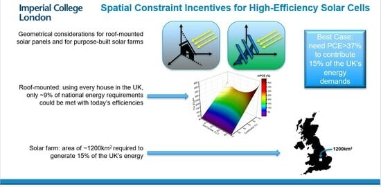
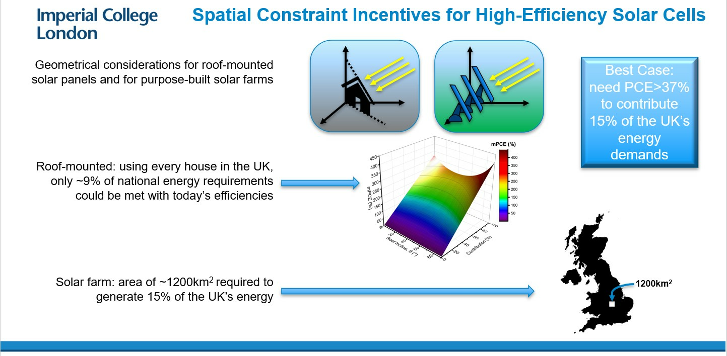
9]. We first look at the option of mounting solar panels on the roofs of houses and calculate, in an idealised model, the limits to the amount of energy that could be generated using the technology with the best commercially available PCE panels.
For definiteness, we use the term contribution to denote the fraction that PVs could supply of the current total UK energy budget and take 15% as the value at which PVs could be said to contribute “significantly” to a sustainable energy future. We also define the term mPCE to denote the minimum PCE required of a piece of PV technology to generate a given contribution. This is all carried out under the most optimistic assumptions of how well a roof-mounted PV system could be implemented in practice.
Finally, we consider the alternative option, which is both much simpler to model and yet politically much more challenging to implement: that of large-scale solar farms. Again, for discussion purposes, we make similarly generous and optimistic assumptions. We present estimates of the land areas that would be required to generate a significant contribution.
2. Methods
2.1. Description of the Model
Our calculations here were directly impacted by three angles that relate to how solar panels are installed, namely the latitude
; the angle to the local horizontal at which the panels are mounted
; and the azimuthal angle of the panels to the meridian
. The way the effective PCE is affected by these is derived geometrically in
Section 2.4 to find an overall obliquity factor suitably averaged through the day and year and, for roof-mounted arrays, through the random distribution of
.
For all calculations involving roof-mounted PVs, the insolation data and statistics on the roof area and energy consumption that have been used are those for the UK or London. The key aspects of the city’s built environment and energy utilisation have been widely and recently surveyed and publicly reported. Also, London typifies the modern mega-city with its high population density. Its temperate climate is fairly typical for the developed world [
10], and its latitude is similarly typical of large population centres, resulting in the key obliquity factors that emerge from the analysis outlined above also being representative of the environments where much of the world’s energy is being consumed.
Our calculations are idealised and are intended for discussion purposes. To this end, at all points where assumptions must be made, we do so in a way that would generate an underestimation of the actual PCE required, even if the degree of underestimation this introduces may be quite significant.
We assume that roof coverage is as complete as practically possible (see
Section 2.3.2) and that all the panels are mounted on roofs that are optimally inclined to the horizontal plane (
Section 2.4.1).
As is discussed more thoroughly in
Section 2.3.2, we had to assume that the statistics for flat dwellers should be processed by assuming that all apartment blocks were only 2 storeys high. In reality of course, many are much taller, and the share of the roof area available to each flat dweller is much lower as a result. Thus, this assumption means that our calculations were likely to considerably overestimate the PV generation capacity in cities.
We also assumed that none of the generated energy was lost in either the storage or transmission schemes (see
Section 2.2).
These issues are commercially and politically sensitive to the point where accessing reliable, unbiased data for analytical studies is problematic. However, by setting our definition of “significance” to only 15% (i.e., rather less than the 60% used by the non-transport sector), we aimed to sidestep these complications by making our conclusions largely independent of what might happen to the transport sector in the future.
2.2. Factors Surrounding the “Perfect Storage” Assumption
In all our calculations, we assumed that no energy generated by a PV system went to waste. For this idealisation to be the case, it must be possible to store any excess energy with no losses for later use when there is a generation deficit. Using the 15% contribution figure for discussion makes this a more practical proposition if one assumes that the overall energy-generating system contains flexible elements whose generating capacity can be switched in and out as the generating capacity of the PV component fluctuates. However, the issue would become progressively more challenging if PVs were to aim for higher contribution levels.
This issue is quantified in the
Supplementary Materials, where we show that a PV system able to generate a 15%
contribution annually may be limited over winter to a
contribution as low as ~3% but become >30% at times over summer. This means other sources would need to provide up to 97% in winter but only ~70% in summer.
At higher assumed
contribution values, storage issues become relevant because the installed capacity required could, in principle, generate more energy in summer than the UK could consume. The excess could be exported or stored. If one assumes that the latter is performed with today’s best battery technology, lithium-ion, then the recovery efficiency is ~80% [
11,
12], and there is a loss due to self-discharging of ~3% per month [
13]. Taking these effects into account, storing enough energy for six months to cope with seasonal variations would increase the corresponding
mPCEs by a factor of 1.5. This is a combination of a 1.25 factor due to the finite energy efficiency and a further factor of 1.2 to account for six months of self-discharge at 3% per month.
2.3. Data Collection
Wherever possible, the data used in the calculations were sourced from official documents such as government reports and statistical tables, and uncertainties were taken from standard deviations or estimated from the data available. To be able to perform the analysis, we required data for the insolation that reached the surface of Earth, the energy consumption of the UK (as a whole and for individual households), and the available rooftop area that could be used to mount solar panels.
2.3.1. Energy: Insolation and Consumption
Insolation data were sourced from NASA’s Projection Of Worldwide Energy Resources (POWER) [
14], which provides insolation data at a given location to 0.5° precision in terms of both latitude and longitude. The data were a daily average for each calendar month of all sky insolation on a horizontal surface using solar climatological datasets which covered the period from July 1983 to June 2005 [
14].
Data for the total annual energy consumption in the UK were taken from the Department for Business, Energy & Industrial Strategy’s (DBEIS’s) Energy Consumption in the UK (ECUK) 2018, using 2017 data [
15]. For calculations that separated homes by the type of dwelling, we used the average annual household consumption from ECUK [
15] and scaled it using electricity data taken from the Household Electricity Survey [
16].
2.3.2. Available Roof Area
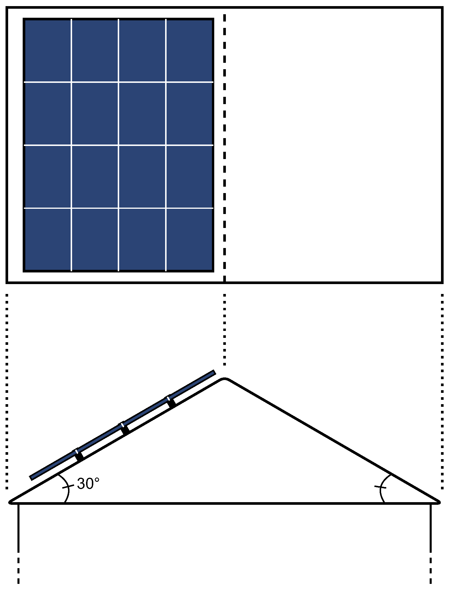
The available roof area was taken from the Energy Saving Trust (EST) [
17], which provides values for a selection of different types of homes. The values given by the EST use dwelling footprints from a report by the BRE Group on behalf of the Department of the Environment, Transport and the Regions [
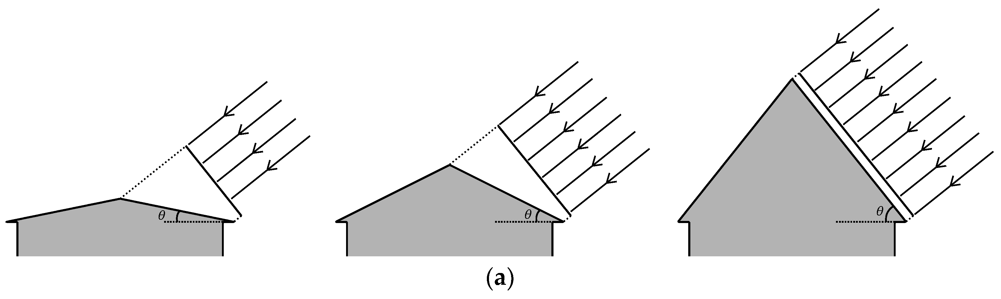
18] and then assume each has a pitched roof with a slope of 30°, meeting in the middle. They assumed that solar panels can be mounted on only one half of the roof, with a further 20% of it being unsuitable. This is shown in
Figure 1. We adjusted the resulting areas quoted by the EST by a factor of
to find the horizontal cross-sectional area (HCSA), which is the cross-sectional area as viewed from directly above. This could then be used in conjunction with the insolation data from NASA POWER, which are for a horizontal surface [
14].
The roof area provided by the EST for a flat was 28 m
2 (giving an HCSA of 24.2 m
2) and was for a “top floor flat” [
17]. We took half that value, as the term “top floor” implies the existence of at least one flat below this one, and the available roof area should be split equally between them. As such, we estimated an increased uncertainty in the HCSA for the flat relative to the other types of homes. In the absence of any further information, for discussion purposes, we must assume that only one flat exists below the top floor, but this means that all the estimates of roof areas available to flat dwellers are likely to be significant overestimates, and the calculations would be strongly biased in favour of lower
mPCE estimates.
Flats make up a large fraction of all households in large cities (~44% in London in 2011 [
19]), and any overestimate in the roof area estimates for a flat will translate to an overestimate by a factor of around half as much for the roof area values for an average home. With blocks of flats often standing at more than three storeys and tower blocks having storeys in the double figures, the roof area per flat was probably quite significantly less than the calculation assumed, but this would be offset by the fact that the calculation ignored the roof areas that might have been available on commercial properties (see
Section 3.1).
2.3.3. Solar Farms and Today’s PCEs
Further data that we researched included the locations of existing solar farms in the UK. We considered the five largest by declared net capacity [
20]. The coordinates for each were taken from Google Maps [
21,
22,
23,
24,
25] using the addresses provided by Ofgem [
20]. We input these coordinates into NASA POWER [
14] and used the location of that which received the highest annual insolation for our calculations of a theoretical solar farm.
Finally, in order to estimate the capability of the solar technology that is currently available, we used six independent web pages that purport to list the most efficient solar panels on the market. The highest reported PCEs ranged from 21.5% to 23.8% [
26,
27,
28,
29,
30,
31]. In this investigation, we took the highest value of 23.8%, as this provided the most optimistic results for today’s technology and therefore challenged our hypothesis most strongly. This value of 23.8% is hereafter referred to as PCE
NOW.
2.4. Geometrical Factors
2.4.1. The Obliquity Factor from Solar Panel Orientation
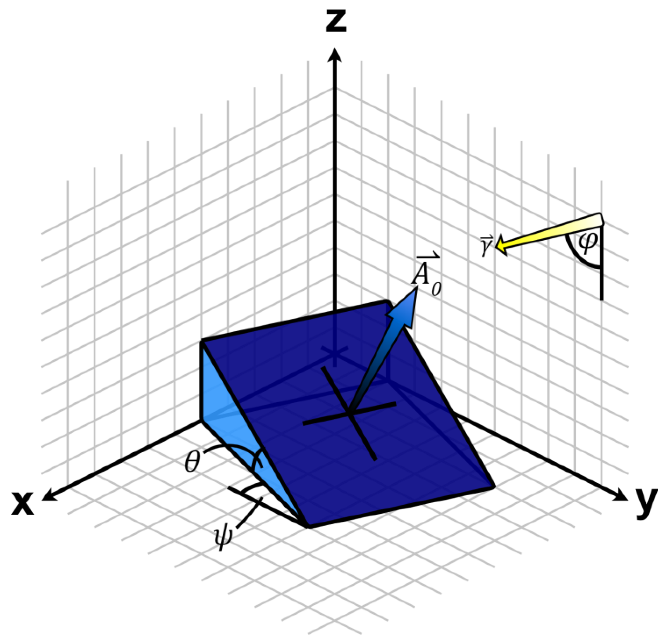
The theoretically ideal orientation of a solar panel—assuming its orientation is fixed—is to mount it at an angle to the horizontal that is equal to the latitude of its location and to have it aligned meridionally, facing the equator. This would mean that the incident solar rays, on average over the course of the year, are normally incident on the panel, and thus the cross-sectional area of the panel is maximised. However, this is not always practical. Especially for roof-mounted solar panels, the angle to the horizontal, and indeed the azimuthal angle to the meridian, are generally fixed by the slope of the roof and the orientation of the house, respectively.
For a solar panel at a location with latitude
, the average angle to the horizontal of incoming solar rays over the course of the year is (
). On top of this, the cross-sectional area of the solar panel that collects sunlight also depends upon the angle of the panels to the horizontal
θ and the azimuthal angle to the meridian
.
Figure 2 illustrates this. By taking the inner product of the vectors labelled
and
in
Figure 2—the normal to the surface of the panel and the average trajectory of incident sunlight, respectively—the cross-sectional area seen by incident sunlight was found to be multiplied by an obliquity factor
, given by
In this study, we assumed that the orientations of houses in the UK were randomly distributed, and thus we averaged this over the appropriate range of azimuthal angles (i.e.,
). The obliquity factor that emerged is then given by
where the
in the denominator is a normalisation factor such that
, meaning the cross-sectional area of the panels when lying flat is unchanged by the obliquity factor. Taking the latitude of London to be
51.5072° [
32], the obliquity factor
—and therefore the insolation received—was maximised to a value of 1.281 for a roof incline of 39°.
If it is possible to align the azimuthal angle directly with the meridian—as would be the case for a free-standing array of solar panels in a solar farm—then the normalised obliquity factor relative to a flat panel is given instead by
which peaks when
, giving a value of
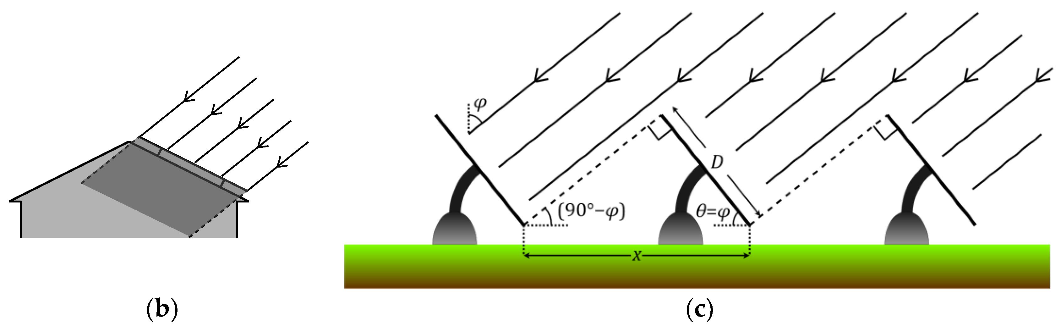
2.4.2. Separation of Rows of Solar Panels
Figure 3 illustrates the effect of tilting solar panels in rooftop and free-standing solar arrays, also highlighting the effect on the space needed between rows of solar panels in a farm. In large-scale solar arrays that have multiple rows of solar panels, tilting the panels at a steeper angle means they must be spaced further apart in order to minimise the shadows cast by one row of panels on the next (
Figure 3c). This is not a problem for roof-mounted arrays, which generally comprise just one row, meaning shadows cast by the panels are irrelevant (
Figure 3b).
For a solar farm, the value of the panel spacing is labelled
in
Figure 3c. When the panels are laid flat (i.e., at
), this is simply equal to the length of the panels
. However, when setting
in order to minimise the amount of material needed (see
Supplementary Materials), the separation
is changed by a factor
, given by
as illustrated in
Figure 3c. This shows that the factor by which the necessary separation of successive rows increases
is the same as the factor by which received insolation increases
. This result means that tilting the panels in a solar farm does not affect the amount of land area needed to generate a given amount of energy. The
spatial efficiency—a measure of the amount of flat land area required to generate a given amount of power for a fixed PCE and fixed insolation on a horizontal surface of an array of consecutive rows of solar panels—is independent of the angle at which the solar panels are tilted to the horizontal.
Note that due to the integral nature of the number of rows of solar panels in a solar farm, this result is not always exact, but the variations for large numbers of rows are small; variations are <1% at all latitudes < 69° for ≥250 rows. With 99% of the world’s population living within 60° of the equator [
33] and the areas involved in these calculations necessitating many rows, this formula is considered to be exact in this paper. More details on the exact variations are given in the
Supplementary Materials.
2.5. Weighted Mean Energy Consumption per Unit Area by House Type
Despite the 28 m
2 given by the EST [
17], the roof area that corresponds to a single flat is likely to be smaller even than the 14 m
2 used here, as blocks of flats are often several stories high, especially in crowded cities. The 2011 census showed that almost half of all households in London were flats at that time [
19], meaning the data for flats are especially important in reaching the value for the average home.
Indeed, we calculated the values for an average home in the UK using a weighted mean consumption per unit HCSA, as shown in
Table 1.
The energy consumptions found for different types of homes using the HES [
16] and the ECUK [
15] gave values for domestic energy use. The domestic sector makes up ~30% of the total energy consumption in the UK [
15], and in order to account for the total energy needs of the UK, these values are upscaled using the ratio of the UK’s total annual energy consumption in all sectors (141 ktoe [
15]) to that in the domestic sector (40 ktoe [
15]). The upscaled value is that which is included in
Table 1.
We then divided the upscaled consumption values by the HCSA for each type of dwelling and weighted them using the number of households of each type, as given by the Census Information Scheme for the 2011 census [
19]. The resulting values were then summed to find a weighted mean annual energy consumption per unit of HCSA.
The same method was used to calculate a weighted mean HCSA for the calculation in
Section 3.2 of the amount of solar panel material that would be needed to install panels on every domestic rooftop in the UK.
3. Results and Discussion
3.1. Contribution from Today’s Best Roof-Mounted Solar Panels
We considered first a scenario with solar panels covering the roofs of every home in the country in order to achieve a grid-level generation capacity that produced a significant
contribution. We did not consider commercial and industrial rooftops, as these buildings are generally not only more densely built (using a smaller area per occupant) but also generally have more storeys, and their roofs are often used to site plant. These issues all result in a small available roof area per occupant. For rooftop calculations, we used the obliquity factor
from Equation (2) to multiply the insolation data from NASA POWER [
14] and took
= 51.5° from [
32].
We supposed that all domestic roofs were covered as fully as possible with solar panels of PCE equal to PCE
NOW. We calculated the power that could be generated by the different classes of dwelling, which gave a
contribution scaled with the average consumption of each type of home. We then calculated the
contribution for an average home by taking a weighted mean of the annual consumption per unit area (as detailed in
Section 2.5).
The results by type of home and for the average home are shown in
Table 2, where we assumed the roof pitch to be the optimal 39° (see
Section 2.4.1) for the latitude of London.
These contributions show that, in this idealisation, the average home could generate a contribution of up to ~9%. This is likely to be a considerable overestimate due to all the assumptions that we made favouring high contributions. We estimated that on average, the effective available roof area per flat might have been another factor of two (i.e., corresponding to a mean block height of four floors), lower than the 14 m2 used here. This would mean a 50% change in the values for the average home. Combining this with the assumptions of perfect storage and an optimal roof incline, we believe that the contribution for PCENOW was more likely to be ⪅5%.
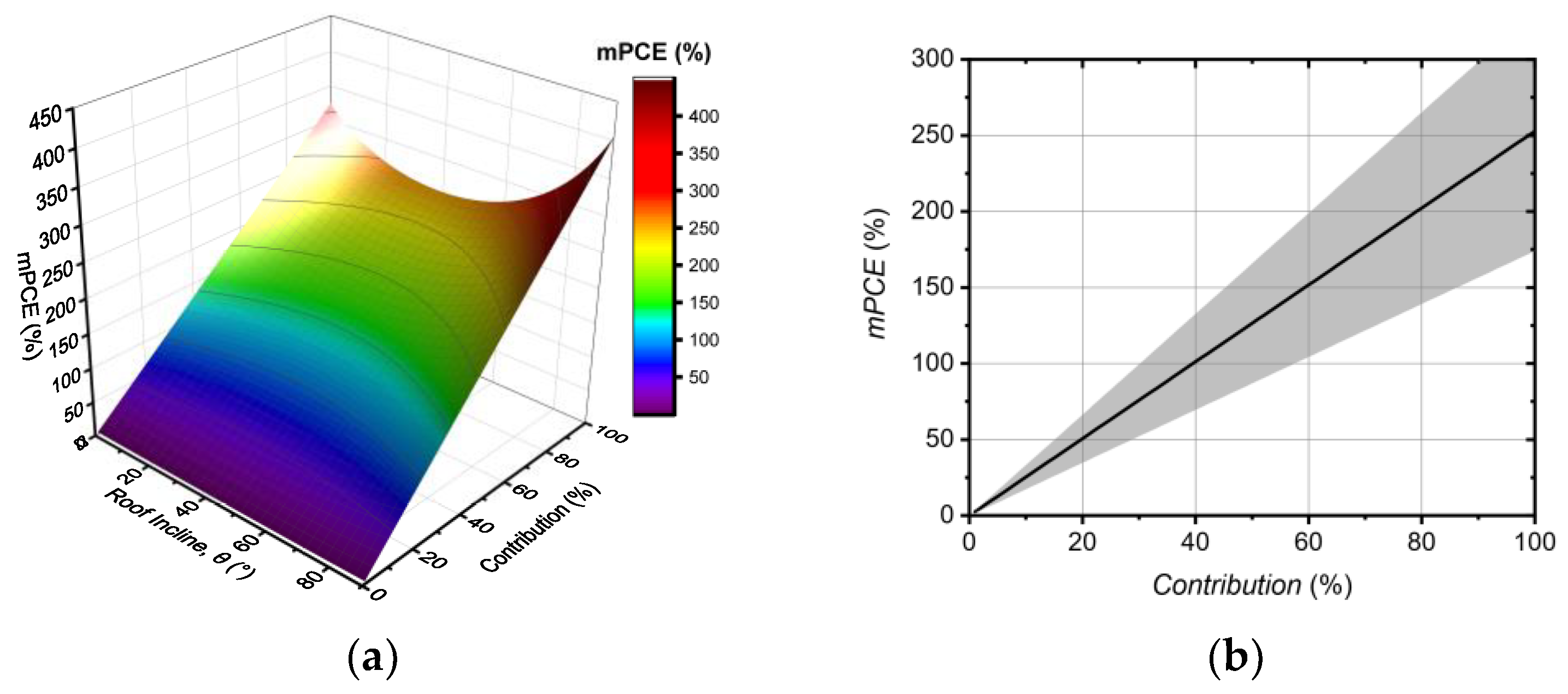
3.2. mPCEs for Roof-Mounted PVs to Provide a 15% Contribution
We repeated the calculations above, first constraining the
contribution and then determining the corresponding
mPCEs that would be required to achieve them. The results for the average home are shown in
Figure 4a as a function of both the roof pitch and
contribution.
Figure 4b shows a cross-section of this at a fixed roof pitch of 39°, the angle corresponding to the lowest
mPCEs. The shaded region in
Figure 4b shows the uncertainty.
In this case, we can see that to generate a contribution of 15%, a PCE of ~37% would be required, which is in excess of the S-Q limit of ~33%. If the PCE were equated to the S-Q limit, then a contribution of ~13% might be generated. However, these values again correspond to the highly optimistic idealised case, with the additional assumption here that all roofs were optimally pitched.
In order to gauge the feasibility of mounting solar panels on all domestic roofs in the UK, we should also consider the quantity and area of the solar panel material that would be needed. The mean available roof area weighted by the number of dwelling types was found to be ~15 m
2. This is the HCSA, while the area of the material actually depends on the absolute area of the inclined roof. Assuming a pitch of 39°, this was ~19.5 m
2. Taking the number of households in the UK to be 28 million (according to a recent government report [
15]), this gave a total panel area of ~550 km
2.
Clearly, this would be a major undertaking. One would hope that there would be quite significant economies of scale, and because of this, present day comparisons based on cost-per-watt estimates for PV technologies must be treated with extreme caution. There is the risk that premature costing exercises could unwittingly rule out research into high-PCE approaches that in fact have the better long-term likelihood of producing a significant contribution to carbon mitigation.
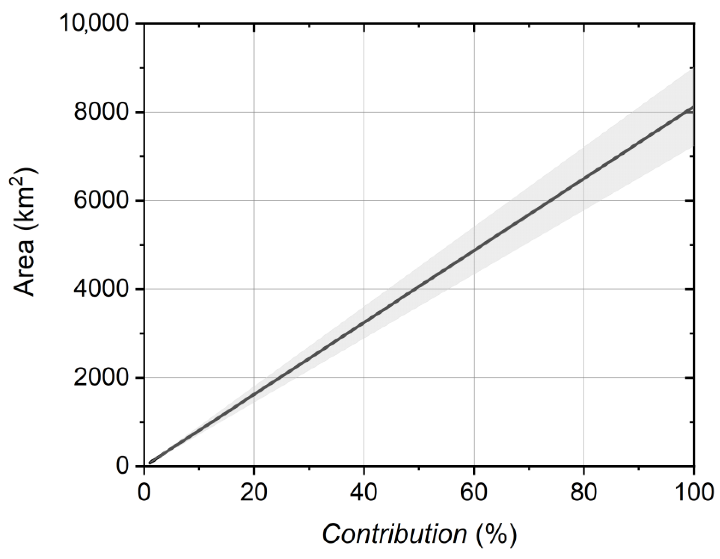
3.3. The Area Needed for a Single Solar Farm in the UK
An alternative to roof-mounted solar arrays is to construct a number of large-scale solar farms. Here, we calculate the land area that would have to be dedicated to a solar farm as a function of
contribution using solar panels of PCE
NOW. In this calculation, we supposed that the panels, if tilted, were built facing meridionally south (
). We therefore used the obliquity factor
from Equation (3) in
Section 2.4.1. The results are shown in
Figure 5, where the shaded area represents an estimate of uncertainty, the main source of which in this case is the energy consumption data.
The calculation was straightforward, with the result being that over 1200 km
2 of new land area would have to be dedicated to solar panels to produce enough energy to fulfil 15% of the energy needs of the UK. As a percentage of the nation’s area, this is small, yet it corresponds to a land area that is comparable to the size of Greater London [
34] and would most likely be impossible to implement either politically or logistically. That said, in this scenario, even small improvements in PCE correspond to large savings in land area. For example, if the PCE were raised from PCE
NOW by one percentage point (from 23.8% to 24.8%), the area needed for a 15%
contribution would decrease by ~50 km
2, roughly the size of a large county town in the UK.
These land area values were unaffected by the tilt of the solar panels according to the constant nature of the
spatial efficiency, a concept discussed in
Section 2.4.2. If the panels were laid flat, then the area of the solar panel material would be the same as the land area (i.e., ~1200 km
2). However, if they were tilted at 52° to the south, this would be reduced by a factor of ~38%, meaning ~750 km
2 of panel material would be needed for the 1200 km
2 farm that would be capable of generating a 15%
contribution.
This is ~250 km
2 more material than would be needed to cover all the UK’s domestic roofs, and this difference arose from two factors. First, this calculation assumed that the farm was in fact large enough to generate a 15%
contribution, whereas there was only enough roof area to generate a ~9%
contribution using the same PCE. Secondly, the obliquity factors were different for the two cases because the orientation of the panels
could be optimised in the farm but was dictated by the spread of house orientations for the rooftop case. There are further details on this calculation in the
Supplementary Materials.
4. Conclusions
Here, we attempted to calculate the fraction of the UK’s energy consumption that could be generated by the best PV technology currently available, factoring in the key consideration of where the panels could realistically be deployed.
This calculation was, necessarily, highly idealised, and it certainly overestimated the possible contribution that today’s PV technology could make. A separate version of this study with more realistic considerations could be of interest in the future. We found that the most efficient solar panels available today, if installed on every domestic roof in the UK, would be able to produce up to ~9% of the UK’s energy. Due to the assumptions made in this analysis, particularly the assumption regarding the roof area available to every flat dweller, we believe that a more realistic figure is less than ~5%.
Using the same generous assumptions, we found that the PCE would need reach values of at least ~37% for roof-mounted solar PVs to contribute 15% of the UK’s energy needs. The same caveats over the available roof area of apartment buildings apply as above, and the real PCEs needed would likely be rather larger still. This already exceeds the Shockley–Queisser theoretical limit of 33% and will only become possible with so-called “third-generation” PV technologies.
Many such technologies employ multi-bandgap and other quantum engineering approaches to circumvent the shortcomings of the single-junction devices that were considered in calculating this limit [
5,
35,
36,
37,
38,
39,
40,
41,
42,
43,
44,
45]. Alternative approaches include hot carrier devices, which increase the photovoltage by harvesting charge carriers before they can thermalise [
46,
47], and the use of concentrator modules to increase the amount of light collected by a solar converter, which can lead to the required efficiencies but comes at increased cost and complexity, and it causes the devices to operate at high temperatures [
48,
49,
50]. All such devices and systems are in the research stage and require further investigation and development to be brought to commercial realisation.
We determined that approximately 1200 km2, an area comparable to the size of Greater London, would be needed for a solar farm to generate 15% of the UK’s energy using the most efficient solar panels currently available.
Our broad conclusion is that independent of the commonly used “dollar-per-watt” economic metric, if solar PVs are to become a significant part of any carbon mitigation strategy, then research and development programmes must target a raw increase in PCEs. Not only are values required that are beyond those currently available, but they are also well beyond the Shockley–Queisser limit of single-bandgap approaches.
Supplementary Materials
The following supporting information can be downloaded at
https://www.mdpi.com/article/10.3390/solar4020009/s1, Section S1: Energy storage and its impact on
mPCEs and land areas; Section S2: Variations in areas of land and material for a solar farm as a function of the panel angle to the horizontal.
Author Contributions
Conceptualisation, K.M.H.; methodology, K.M.H.; software, K.M.H.; validation, K.M.H. and C.C.P.; formal analysis, K.M.H.; investigation, K.M.H.; resources, K.M.H. and C.C.P.; data curation, K.M.H.; writing—original draft preparation, K.M.H.; writing—review and editing, K.M.H. and C.C.P.; visualisation, K.M.H.; supervision, C.C.P.; project administration, K.M.H. and C.C.P.; funding acquisition, C.C.P. All authors have read and agreed to the published version of the manuscript.
Funding
This work was funded by the UK Engineering and Physical Sciences Research Council, grant no. EP/K029398/1.
Institutional Review Board Statement
Not applicable.
Informed Consent Statement
Not applicable.
Data Availability Statement
Data are available from the authors upon reasonable request.
Conflicts of Interest
The authors declare no conflicts of interest. The funders had no role in the design of the study; in the collection, analyses, or interpretation of data; in the writing of the manuscript; or in the decision to publish the results.
References
- Kojima, A.; Teshima, K.; Shirai, Y.; Miyasaka, T. Organometal Halide Perovskites as Visible-Light Sensitizers for Photovoltaic Cells. J. Am. Chem. Soc. 2009, 131, 6050–6051. [Google Scholar] [CrossRef]
- Cheng, Z.; Lin, J. Layered organic-inorganic hybrid perovskites: Structure, optical properties, film preparation, patterning and templating engineering. CrystEngComm. 2010, 12, 2646–2662. [Google Scholar] [CrossRef]
- Jiang, Q.; Chu, Z.; Wang, P.; Yang, X.; Liu, H.; Wang, Y.; Yin, Z.; Wu, J.; Zhang, X.; You, J. Planar-Structure Perovskite Solar Cells with Efficiency beyond 21%. Adv. Mater. 2017, 29, 1703852. [Google Scholar] [CrossRef]
- Kim, H.-S.; Lee, C.-R.; Im, J.-H.; Lee, K.-B.; Moehl, T.; Marchioro, A.; Moon, S.-J.; Humphry-Baker, R.; Yum, J.-H.; Moser, J.E.; et al. Lead Iodide Perovskite Sensitized All-Solid-State Submicron Thin Film Mesoscopic Solar Cell with Efficiency Exceeding 9%. Sci. Rep. 2012, 2, 591. [Google Scholar] [CrossRef]
- Oxford PV. Oxford PV Sets New Solar Cell World Record, Oxford PV. 2023. Available online: https://www.oxfordpv.com/news/oxford-pv-sets-new-solar-cell-world-record (accessed on 12 January 2024).
- Ball, J.M.; Petrozza, A. Defects in perovskite-halides and their effects in solar cells. Nat. Energy 2016, 1, 16149. [Google Scholar] [CrossRef]
- Shockley, W.; Queisser, H.J. Detailed Balance Limit of Efficiency of p-n Junction Solar Cells. J. Appl. Phys. 1961, 32, 510–519. [Google Scholar] [CrossRef]
- Rühle, S. Tabulated values of the Shockley-Queisser limit for single junction solar cells. Sol. Energy 2016, 130, 139–147. [Google Scholar] [CrossRef]
- Green, M.A.; Bremner, S.P. Energy conversion approaches and materials for high-efficiency photovoltaics. Nat. Mater. 2016, 16, 23–34. [Google Scholar] [CrossRef] [PubMed]
- Solargis, Global Solar Atlas 2.0. 2023. Available online: https://globalsolaratlas.info/map (accessed on 12 January 2024).
- Zhang, P.; Du, C.; Yan, F.; Kang, J. Influence of practical complications on energy efficiency of the vehicle’s lithium-ion batteries. In Proceedings of the 2011 International Conference on Electric Information and Control Engineering, Wuhan, China, 15–17 April 2011; pp. 2278–2281. [Google Scholar]
- Eftekhari, A. Energy efficiency: A critically important but neglected factor in battery research. Sustain. Energy Fuels 2017, 1, 2053–2060. [Google Scholar] [CrossRef]
- Vetter, M.; Lux, S. Rechargeable Batteries with Special Reference to Lithium-Ion Batteries. In Storing Energy; Elsevier: Oxford, UK, 2016; pp. 205–225. [Google Scholar] [CrossRef]
- NASA Langley Research Center, POWER Data Access Viewer. 2018. Available online: https://power.larc.nasa.gov/data-access-viewer/ (accessed on 12 January 2024).
- Department for Business Energy & Industrial Strategy, Energy Consumption in the UK (ECUK) 2018 Data Tables. 2018. Available online: https://webarchive.nationalarchives.gov.uk/ukgwa/20190509005513/https://www.gov.uk/government/statistics/energy-consumption-in-the-uk (accessed on 12 January 2024).
- Zimmerman, J.-P.; Evans, M.; Griggs, J.; King, N.; Harding, L.; Roberts, P.; Evans, C. Household Electricity Survey A Study of Domestic Electrical Product Usage. 2012. Available online: https://assets.publishing.service.gov.uk/government/uploads/system/uploads/attachment_data/file/208097/10043_R66141HouseholdElectricitySurveyFinalReportissue4.pdf (accessed on 25 February 2024).
- Energy Saving Trust, Solar Energy Calculator Sizing Guide. 2015. Available online: https://energysavingtrust.org.uk/tool/solar-energy-calculator/ (accessed on 12 January 2024).
- Iles, P.J. Standard Dwellings for Energy Modelling; Client Report CR444/98; Building Research Establishment Ltd.: Garston, UK, 1999. [Google Scholar]
- GLA Intelligence Census Information Scheme, 2011 Census Housing Characteristics. 2013. Available online: https://data.london.gov.uk/download/2011-census-housing/377bcc89-fab4-4f88-a69f-10a2570cbde5/2011-census-housing-characteristics.pdf (accessed on 12 January 2024).
- Ofgem. Ofgem Renewables and CHP Register. 2007. Available online: https://www.renewablesandchp.ofgem.gov.uk/Public/ReportManager.aspx?ReportVisibility=1&ReportCategory=0 (accessed on 12 January 2024).
- Google. Google Maps—Shotwick Solar Park. 2024. Available online: https://www.google.com/maps/place/Shotwick+Solar+Park/@53.2385404,-3.0204782,17z/data=!3m1!4b1!4m5!3m4!1s0x487adbb6a8432c33:0x3faa669894904fac!8m2!3d53.2385404!4d-3.0182895 (accessed on 12 January 2024).
- Google. Google Maps—West Raynham Solar Farm. 2024. Available online: https://www.google.com/maps/place/West+Raynham+Solar+Farm/@52.7874045,0.7399422,17z/data=!3m1!4b1!4m5!3m4!1s0x47d783aa7ac52a71:0xf9c9cb1d996c041!8m2!3d52.7874045!4d0.7421309 (accessed on 12 January 2024).
- Google. Google Maps—Eveley Farm. 2024. Available online: https://www.google.com/maps/place/Eveley+Farm/@51.093952,-0.8895097,17z/data=!3m1!4b1!4m5!3m4!1s0x487430d56909b8a7:0xbf25e5fff47d9c0d!8m2!3d51.093952!4d-0.887321 (accessed on 12 January 2024).
- Google. Google Maps—National Collections Centre. 2024. Available online: https://www.google.com/maps/place/National+Collections+Centre/@51.5107303,-1.8148946,17z/data=!3m1!4b1!4m5!3m4!1s0x487144a87ad0f6b9:0x30375e0b110613b9!8m2!3d51.510727!4d-1.8127059 (accessed on 12 January 2024).
- Google. Google Maps—MOD Lyneham, 2024. Available online: https://www.google.com/maps/place/MOD+Lyneham/@51.5055658,-1.9714883,17z/data=!3m1!4b1!4m5!3m4!1s0x487168869f38ccb5:0xab41dd8fb3e8c7c3!8m2!3d51.5055658!4d-1.9692996 (accessed on 12 January 2024).
- Clissit, C. Most Efficient Solar Panels 2020. Eco Experts. 2020. Available online: https://www.theecoexperts.co.uk/solar-panels/most-efficient (accessed on 23 March 2020).
- Aggarwal, V. What Are the Most Efficient Solar Panels on the Market? Solar Panel Cell Efficiency Explained. Energy Sage. 2020. Available online: https://news.energysage.com/what-are-the-most-efficient-solar-panels-on-the-market/ (accessed on 23 March 2020).
- Chakrabarti, S. Top 10 Solar Panels in the UK in 2019. Solar Feeds. 2019. Available online: https://solarfeeds.com/top-solar-panels-in-the-uk/ (accessed on 23 March 2020).
- How Efficient Are Solar Panels? Househ. Quotes. 2019. Available online: https://householdquotes.co.uk/how-efficient-are-solar-panels/ (accessed on 23 March 2020).
- Svarc, J. Most Efficient Solar Panels. Clean Energy Reviews. 2019. Available online: https://www.cleanenergyreviews.info/blog/most-efficient-solar-panels (accessed on 23 March 2020).
- What is the Most Efficient Solar Panel. Joju Solar. 2019. Available online: https://www.jojusolar.co.uk/2017/06/06/high-efficiency-solar-panel/ (accessed on 23 March 2020).
- Wikimedia Tool Labs, GeoHack—London. 2024. Available online: https://geohack.toolforge.org/geohack.php?pagename=London%5C¶ms=51_30_26_N_0_7_39_W_region:GB_type:city(8825000) (accessed on 12 January 2024).
- Kummu, M.; Varis, O. The world by latitudes: A global analysis of human population, development level and environment across the north–south axis over the past half century. Appl. Geogr. 2011, 31, 495–507. [Google Scholar] [CrossRef]
- Natural England, Access to Nature: Regional Targeting Plan—London. 2009. Available online: https://webarchive.nationalarchives.gov.uk/20140605113419/http://www.naturalengland.org.uk/Images/London-rtp_tcm6-4496.pdf (accessed on 12 January 2024).
- Aihara, T.; Tayagaki, T.; Nagato, Y.; Okano, Y.; Sugaya, T. Investigation of the open-circuit voltage in wide-bandgap InGaP-host InP quantum dot intermediate-band solar cells. Jpn. J. Appl. Phys. 2018, 57, 04FS04. [Google Scholar] [CrossRef]
- Vaquero-Stainer, A.; Yoshida, M.; Hylton, N.P.; Pusch, A.; Curtin, O.; Frogley, M.; Wilson, T.; Clarke, E.; Kennedy, K.; Ekins-Daukes, N.J.; et al. Semiconductor nanostructure quantum ratchet for high efficiency solar cells. Commun. Phys. 2018, 1, 7. [Google Scholar] [CrossRef]
- Yamaguchi, M.; Lee, K.-H.; Araki, K.; Kojima, N. A review of recent progress in heterogeneous silicon tandem solar cells. J. Phys. D Appl. Phys. 2018, 51, 133002. [Google Scholar] [CrossRef]
- Delamarre, A.; Suchet, D.; Cavassilas, N.; Okada, Y.; Sugiyama, M.; Guillemoles, J.-F. Non-ideal nanostructured intermediate band solar cells with an electronic ratchet. In Physics, Simulation, and Photonic Engineering of Photovoltaic Devices VII; SPIE OPTO, SPIE: San Francisco, CA, USA, 2018; p. 5. [Google Scholar]
- Geisz, J.F.; France, R.M.; Schulte, K.L.; Steiner, M.A.; Norman, A.G.; Guthrey, H.L.; Young, M.R.; Song, T.; Moriarty, T. Six-junction III–V solar cells with 47.1% conversion efficiency under 143 Suns concentration. Nat. Energy 2020, 5, 326–335. [Google Scholar] [CrossRef]
- Kita, T.; Maeda, T.; Harada, Y. Carrier dynamics of the intermediate state in InAs/GaAs quantum dots coupled in a photonic cavity under two-photon excitation. Phys. Rev. B 2012, 86, 35301. [Google Scholar] [CrossRef]
- Martí, A.; Antolín, E.; Stanley, C.R.; Farmer, C.D.; López, N.; Díaz, P.; Cánovas, E.; Linares, P.G.; Luque, A. Production of Photocurrent due to Intermediate-to-Conduction-Band Transitions: A Demonstration of a Key Operating Principle of the Intermediate-Band Solar Cell. Phys. Rev. Lett. 2006, 97, 247701. [Google Scholar] [CrossRef]
- Okada, Y.; Ekins-Daukes, N.J.; Kita, T.; Tamaki, R.; Yoshida, M.; Pusch, A.; Hess, O.; Phillips, C.C.; Farrell, D.J.; Yoshida, K.; et al. Intermediate band solar cells: Recent progress and future directions. Appl. Phys. Rev. 2015, 2, 21302. [Google Scholar] [CrossRef]
- Okada, Y.; Morioka, T.; Yoshida, K.; Oshima, R.; Shoji, Y.; Inoue, T.; Kita, T. Increase in photocurrent by optical transitions via intermediate quantum states in direct-doped InAs/GaNAs strain-compensated quantum dot solar cell. J. Appl. Phys. 2011, 109, 24301. [Google Scholar] [CrossRef]
- Rienäcker, M.; Schnabel, M.; Warren, E.; Merkle, A.; Schulte-Huxel, H.; Klein, T.; van Hest, M.F.A.M.; Steiner, M.A.; Geisz, J.F.; Kajari-Schröder, S.; et al. Mechanically Stacked Dual-Junction and Triple-Junction III-V/Si-IBC Cells with Efficiencies of 31.5% and 35.4%. In Proceedings of the 33rd European Photovoltaic Solar Energy Conference and Exhibition, Amsterdam, The Netherlands, 25–29 September 2017. [Google Scholar] [CrossRef]
- Tanaka, T.; Matsuo, K.; Saito, K.; Guo, Q.; Tayagaki, T.; Yu, K.M.; Walukiewicz, W. Cl-doping effect in ZnTe(1-x)Ox highly mismatched alloys for intermediate band solar cells. J. Appl. Phys. 2019, 125, 243109. [Google Scholar] [CrossRef]
- Conibeer, G.; Green, M.; Corkish, R.; Cho, Y.; Cho, E.-C.; Jiang, C.-W.; Fangsuwannarak, T.; Pink, E.; Huang, Y.; Puzzer, T.; et al. Silicon nanostructures for third generation photovoltaic solar cells. Thin Solid Films 2006, 511–512, 654–662. [Google Scholar] [CrossRef]
- Spanier, J.E.; Fridkin, V.M.; Rappe, A.M.; Akbashev, A.R.; Polemi, A.; Qi, Y.; Gu, Z.; Young, S.M.; Hawley, C.J.; Imbrenda, D.; et al. Power conversion efficiency exceeding the Shockley–Queisser limit in a ferroelectric insulator. Nat. Photonics 2016, 10, 611–616. [Google Scholar] [CrossRef]
- Araújo, G.L.; Martí, A. Absolute limiting efficiencies for photovoltaic energy conversion. Sol. Energy Mater. Sol. Cells 1994, 33, 213–240. [Google Scholar] [CrossRef]
- Philipps, S.P.; Bett, A.W.; Horowitz, K.; Kurtz, S. Current Status of Concentrator Photovoltaic (CPV) Technology; National Renewable Energy Lab.(NREL): Golden, CO, USA, 2015. [Google Scholar] [CrossRef]
- Tang, J.; Ni, H.; Peng, R.-L.; Wang, N.; Zuo, L. A review on energy conversion using hybrid photovoltaic and thermoelectric systems. J. Power Sources 2023, 562, 232785. [Google Scholar] [CrossRef]
| Disclaimer/Publisher’s Note: The statements, opinions and data contained in all publications are solely those of the individual author(s) and contributor(s) and not of MDPI and/or the editor(s). MDPI and/or the editor(s) disclaim responsibility for any injury to people or property resulting from any ideas, methods, instructions or products referred to in the content. |
© 2024 by the authors. Licensee MDPI, Basel, Switzerland. This article is an open access article distributed under the terms and conditions of the Creative Commons Attribution (CC BY) license (https://creativecommons.org/licenses/by/4.0/).


