A Novel Statistical Framework for Optimal Sizing of Grid-Connected Photovoltaic–Battery Systems for Peak Demand Reduction to Flatten Daily Load Profiles

Abstract

Integrating photovoltaic (PV) systems plays a pivotal role in the global shift toward renewable energy, offering significant environmental benefits. However, the PV installation should provide financial benefits for the utilities. Considering that the utility companies often incur costs for both energy and peak demand, PV installations should aim to reduce both energy and peak demand charges. Although PV systems can reduce energy needs during the day, their effectiveness in reducing peak demand, particularly in the early morning and late evening, is limited, as PV generation is zero or negligible at those times. To address this limitation, battery storage systems are utilized for storing energy during off-peak hours and releasing it during peak times. However, finding the optimal size of PV and the accompanying battery remains a challenge. While valuable optimization models have been developed to determine the optimal size of PV–battery systems, a certain gap remains where peak demand reduction has not been sufficiently addressed in the optimization process. Recognizing this gap, this study proposes a novel statistical model to optimize PV–battery system size for peak demand reduction. The model aims to flatten 95% of daily peak demands up to a certain demand threshold, ensuring consistent energy supply and financial benefit for utility companies. A straightforward and effective search methodology is employed to determine the optimal system sizes. Additionally, the model’s effectiveness is rigorously tested through a modified Monte Carlo simulation coupled with time series clustering to generate various scenarios to assess performance under different conditions. The results indicate that the optimal PV–battery system successfully flattens 95% of daily peak demand with a selected threshold of 2000 kW, yielding a financial benefit of USD 812,648 over 20 years.

1. Introduction

The move toward renewable energy is a response to growing environmental concerns and the limited supply of non-renewable resources [1]. Photovoltaic (PV) systems are becoming increasingly important in this shift because of their ability to use solar energy, which is both abundant and environmentally friendly [2]. Considerable efforts are underway to improve the PV technology. For instance, the authors of [3,4] have shown that monolithic perovskite/silicon tandem solar cells recently achieved a certified efficiency of 29.1%. Recent advancements have significantly improved PV module lifetimes and their ability to perform optimally even in harsh environmental conditions [5]. Despite the advancement in PV systems, they still present significant technological and economic challenges [6]. The installation of PV systems must yield financial benefits for utilities and meet technical requirements. In most instances, utility companies incur costs for both energy and peak demand. Therefore, PV installations must not only reduce the energy needed but also reduce the peak demand. Energy requirements can be reduced whenever PV systems generate electricity, resulting in financial benefits for utility companies. However, reducing peak demand with PV systems requires additional analysis, with consideration of various factors. For example, during winter days, peak demand often occurs in the early morning when there is negligible or no PV generation [7]. Consequently, on such days, PV installations do not contribute to peak demand reduction. In addition, peak demand may coincide with minimal PV generation during certain days in the spring and fall, limiting the utility benefits.

Considering that peak demand charges are typically high, it is important to leverage PV generation for peak demand reduction. To address this challenge, battery storage systems, which have seen significant advancements in efficiency and capacity, can be potentially useful [8]. By shifting energy from off-peak to peak hours, batteries can reduce peak demand, thereby providing greater financial benefits for utility companies. While the use of energy storage systems can aid in reducing peak demands and enhancing financial benefits, it also introduces additional costs associated with battery installation and energy losses during charging and discharging. Therefore, determining the optimal size of PV–battery systems is critical to satisfy both technical and economic considerations. Many studies have been conducted to identify the optimal size of grid-connected PV–battery systems [9].

1.1. PV–Battery Optimal Sizing Approaches

The methodologies explored in the existing literature for optimizing PV–battery systems can be categorized, as in the following sections.

1.1.1. Single-Objective Optimization

Single-objective optimization focuses on optimizing a single aspect of the PV–battery system, such as cost minimization, energy efficiency, or reliability [10]. The authors of [11] developed a single-objective-function model to maximize energy savings in PV–battery systems. Their findings suggested that residents could save 5% of their total electricity load without storage and 14% with storage. The researchers in [12] formulated a model for the economic assessment of residential PV systems with lithium-ion batteries. Their analysis showed that optimal sizing can make these systems more affordable than PV alone. In [13], a mixed-integer nonlinear programming optimization model was created to optimize the operation and investment of PV–battery systems. The study revealed that the temporal resolution of electrical load and PV generation profiles significantly influences self-consumption and optimal system sizing. The authors of [14] proposed a methodology for determining the optimal size of PV–battery systems, focusing on the overall cost throughout the project lifetime. This approach, validated against realistic test cases, provides an economic analysis to ensure the investment feasibility. While single-objective optimization methods are effective in determining the optimal PV–battery system, they might not adequately address other crucial aspects of PV–battery systems. This narrow focus can result in solutions that may not be optimal when considering the broader operational needs and challenges of PV–battery systems. To address this limitation, multi-objective optimization approaches have been developed.

1.1.2. Multi-Objective Function Optimization

Multi-objective function optimization involves optimizing multiple objectives simultaneously, such as cost, efficiency, reliability, and environmental impact [15]. The authors of [16] developed a multi-objective optimization model for PV and battery energy storage systems, implemented using particle swarm optimization. The objectives included loss minimization, voltage, and load ability improvement. The authors of [17] developed a multi-objective optimization for grid-connected PV–battery systems, utilizing machine learning techniques. The objective functions included minimizing energy bought from the utility grid, maximizing the battery state of charge, and reducing carbon dioxide emissions. In [18], a scenario-based multi-objective optimization for a rural PV–battery system, focusing on economic gains and grid interaction, was developed. Findings showed an 87% improvement in grid interaction smoothness, highlighting its effectiveness in various scenarios and weather conditions. Similarly, Song, Guan, and Cheng [19] proposed a multi-objective optimization strategy for home energy management systems, including PV and battery energy storage, emphasizing the integration of sustainable energy sources into the grid. However, a significant limitation shared by both single- and multi-objective optimization methods is their lack of consideration for uncertainty. Real-world PV–battery systems operate under a variety of uncertain conditions, including fluctuating solar irradiance and changing load demands. The failure to incorporate these uncertainties into the optimization models can limit the applicability and resilience of the proposed solutions in real-word applications. To address this critical gap, stochastic and robust optimization methods were typically utilized.

1.1.3. Stochastic Optimization

Stochastic optimization can be used to determine the optimal size and operation of PV–battery systems under uncertain conditions [20]. By considering a range of possible scenarios, such as varying levels of solar irradiance and changes in energy demand, this method allows for the design of systems that are not only cost-effective but also resilient to changes in environmental conditions and energy market dynamics [21]. The authors of [22] employed a stochastic optimization approach to determine the optimal size of the PV–battery system, focusing on minimizing system unavailability and cost. Based on their findings, PV panel costs and efficiency significantly affect the optimal system. Using stochastic optimization, the authors of [23] developed a model for sizing battery storage integrated with PV systems, aiming to minimize the battery cost and grid energy import. Their results indicated that combining financial and technical objectives is crucial for achieving economically feasible PV–battery sizing. According to the authors of [24], an integrated stochastic framework was developed to optimize the design and operation of PV–battery systems. In that study, feed-in tariffs and unit costs played a major role in determining PV–battery sizes. While stochastic optimization provides a robust framework for dealing with uncertainties, these methods often require large numbers of data and fitting the data into known probability distribution functions (PDFs) that can be complex and computationally intensive [25].

1.1.4. Robust Optimization

On the other hand, robust optimization addresses uncertainty by establishing parameter bounds. They are particularly useful when data are insufficient, or when probability distributions are either unknown or fitting them is statistically insignificant [26]. Robust optimization is a new method in PV–battery optimization that constructs solutions to perform effectively within a range of uncertainty, defined by intervals, ensuring consistency and resilience against variations in input data and model parameters [27]. In [28], a two-stage robust optimization model was presented for optimal sizing of PV systems with battery units. It addresses PV generation and load uncertainties using polyhedral uncertainty sets. The authors of [29] conducted robust optimization for grid-connected PV–battery systems. It emphasized the importance of considering real-world uncertainties in system design. The study demonstrated a trade-off between minimizing the levelized cost of electricity mean and its standard deviation, using Pareto sets of optimized designs. While robust optimization offers a pragmatic approach to managing uncertainty, it tends to yield overly conservative solutions. Besides, accurately determining the appropriate uncertainty bounds is challenging, which can significantly impact the efficiency and feasibility of the optimized system.

Despite these optimization approaches providing valuable insights into optimizing PV–battery systems, especially for grid-connected applications, a certain gap remains. Peak demand has not been sufficiently integrated into existing optimization frameworks. This oversight is particularly crucial considering that utility companies often incur substantial costs for peak demand. Recognizing this gap, this study proposes novel statistical models aimed at comprehensively addressing the optimization of grid-connected PV–battery systems, with a particular emphasis on peak demand reduction. The models enable utility companies to design PV–battery systems capable of effectively flattening 95% of the daily load demand profiles up to a predefined threshold. This threshold is determined by the utilities, considering their operational capacity and risk management considerations.

The optimization process for PV–battery systems traditionally relies on historical data, assuming the parameters determining the optimal configurations are deterministic. However, key factors, such as demand and solar irradiance, are inherently uncertain, and their variability significantly impacts the optimization process. Failing to consider such uncertainties may compromise the effectiveness of the optimal PV–battery system, and potentially lead to a non-optimal peak demand reduction, compromised utility benefits, and even system instability [30]. Single- and multi-objective optimization problems have often been approached by assuming deterministic data. Additionally, the challenges of accurately determining appropriate uncertainty bounds in robust optimization, alongside the complexities and computational intensities of fitting data into known PDFs in stochastic optimization, highlight the limitations of the current methodologies. Recognizing the critical importance of accounting for uncertainty in the optimization process and the limitations associated with robust and stochastic optimization, this study utilizes a modified Monte Carlo simulation. Traditional Monte Carlo simulations, which treat uncertain parameters independently, may produce unrealistic scenarios. For example, they may generate a winter load profile alongside a summer solar irradiance profile. To remedy this, the modified Monte Carlo simulation employs time series clustering techniques to recognize the complex interdependencies between solar irradiance and load demand. By grouping similar demand and solar irradiance profiles into clusters and using conditional probabilities between the load demand and solar irradiance clusters, more realistic scenarios are generated.

In this study, actual demand and solar irradiance data from the City of Greensburg, Kansas, USA, were collected to establish the methodology. Initially, a specific PV size was selected, and modified daily load profiles were generated by subtracting the original load from the PV generation for that PV size. The needed batteries were calculated for each day to flatten the daily loads. Then, a range of battery sizes was chosen to calculate the updated daily peak demands after PV–battery installation by taking advantage of the required daily batteries. The updated peaks were then represented in histograms corresponding to each PV–battery combination and fitted with appropriate PDFs. When the 95th percentile value of a PDF matched the desired utility threshold, the corresponding PV and battery sizes were considered optimal. Otherwise, new PDF parameters were determined to align the 95th percentile with the utility threshold. By iterating this process across various PV sizes, we identified optimal combinations of PV–battery systems capable of flattening 95% of daily peaks up to a certain demand threshold. A financial analysis was then conducted to identify the most economically beneficial configurations. Finally, a modified Monte Carlo simulation, coupled with time series clustering, was employed to rigorously test the optimal system under various load and solar irradiance conditions. The proposed model provides a practical and efficient approach for determining the optimal size of PV–battery systems, specifically tailored for utilities connected to the grid and incurring peak demand charges. The organizational flowchart of the simulation procedure in this study is shown in Figure 1.

1.2. Contributions

The main contributions of this study can be summarized as follows:

• Development of a novel statistical model. We introduce a new statistical model specifically designed for optimizing PV–battery system sizes, with a primary focus on peak demand reduction. This model addresses a critical gap in the current literature by considering both energy consumption and peak demand costs, which are essential factors for utility companies.
• Incorporation of a modified Monte Carlo simulation. The study utilizes a modified Monte Carlo simulation approach to generate realistic and varied operational scenarios. This methodological innovation allows for a better understanding of PV–battery system performance under diverse conditions, enhancing the robustness of our optimization model.
• Operational and financial analysis for utilities. By providing a method to effectively flatten up to 95% of daily load demand profiles, the model offers a practical tool for utility companies. It enables them to make informed decisions regarding the optimal sizing of PV–battery systems, balancing technical feasibility with financial viability.

2. Materials and Methods

This section provides an overview of the techniques used to determine the optimal size of the PV–battery system.

2.1. Data Collection and Assumptions

For this study, actual solar irradiance and load demand data were collected over three years, from 2019 to 2021, for the City of Greensburg, Kansas, USA. The data were collected on an hourly basis. Tax credits of 30% are available for PV–battery installation costs. In the case of replacement batteries acquired after their lifetime, a tax credit is not available. It is assumed that daily load demands are flattened up to a predefined threshold of 2000 kW. Additionally, the quantity values utilized in this study are presented in

Table 1. The quantity values used in this study.

PV Module (USD/W) 0.35	Inverter (USD/W) 0.04	Equipment (USD/W) 0.18
Overhead (USD/W)	O&M (USD/kW)	Transformer (USD)
0.1	15	150,000
Energy cost (USD/kWh)	Power cost (USD/kW)	Tax credit (%)
0.025	22	30
Initial battery (USD/kWh)	Replacement battery (USD/kWh)	Project lifetime
150	100	20 years
Labor (USD/W)	Discount rate	Battery roundtrip efficiency
0.1	0.08	0.9025
Inverter coefficient	Battery efficiency	Battery utilization
1.2	0.95	0.7

.

2.2. PV–Battery System Component Model

This study examined a system comprised of silicon-based solar panels, inverters, transformers, and batteries. The solar panels are responsible for converting solar energy into electrical energy [31]. Considering a PV system with a size of X kW, the DC output power of this PV system at any given hour, h, can be expressed by the equation [32]:

$$PV(h)=\frac{X}{1000}\times I(h)$$

(1)

where, $PV(h)$ represents the DC output power of the PV system in kW at hour h, $I(h)$ denotes the solar irradiance in $\mathrm{W}/{\mathrm{m}}^2$ at hour h, and 1000 is the solar constant in $\mathrm{W}/{\mathrm{m}}^2$.

The inverters convert the DC electricity generated by the solar panels into AC electricity. The performance of the inverter is modeled as follows [33]:

$$P_{inv}(h)=PV(h)·{\eta }_{inv}$$

(2)

where, $P_{inv}(h)$ represents the AC output power of the inverter and ${\eta }_{inv}$ is the inverter efficiency.

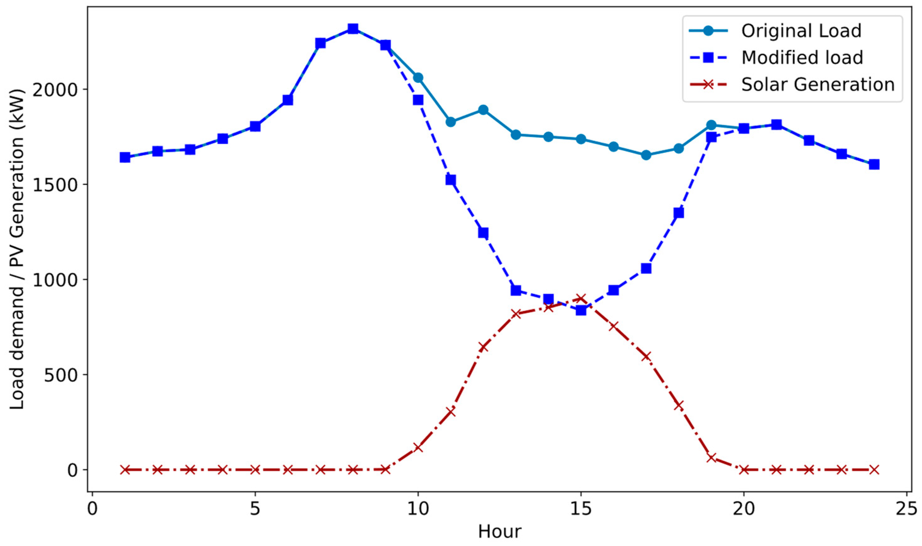
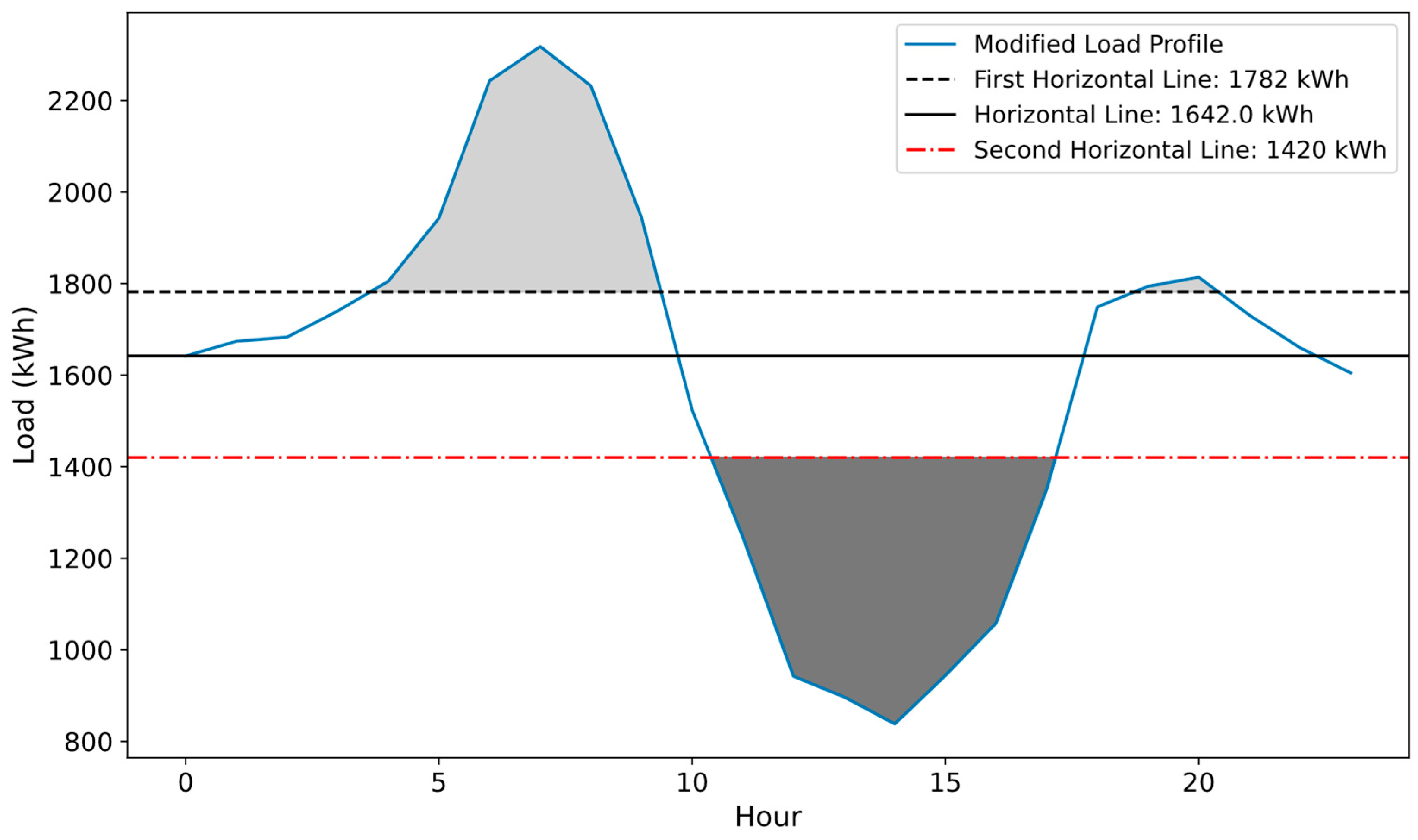
2.3. Required Daily Battery Size

The primary task of the battery in the PV–battery system is to store excess energy generated by the PV panels during peak sunlight hours and provide energy during periods of high demand. To develop the proposed methodology, the first step was to calculate the daily load demand after PV installation, referred to as modified daily load profiles. Initially, a range of PV sizes, denoted from X₁ to X_n kW, was considered. For a PV system of X kW, the output AC power is given by Equation (2). We then generated the modified daily load profiles by subtracting PV generation from the original load profile for each day. For example, Figure 2 illustrates the original load, PV generation, and the modified load, derived by subtracting PV generation from the original load for a PV size of 2000 kW on a selected day in December 2020.

After calculating the modified load profiles for PV sizes ranging from X₁ to X_n for all days, the next step involved determining the required daily battery sizes. These are sizes that can effectively flatten the modified daily load profiles. This calculation assumes a daily battery cycle, which means the battery charges and discharges within a day [7]. To determine the required daily battery size, a horizontal line was drawn across the modified daily load profile so that the area above the line was equal to the roundtrip efficiency multiplied by the area below the line:

$$\mathrm{Area} \mathrm{above} \mathrm{the} \mathrm{line}= \mathrm{Area} \mathrm{below} \mathrm{the} \mathrm{line}\times \mathrm{Battery} \mathrm{roundtrip} \mathrm{efficiency}$$

(3)

The lower area, corresponding to energy drawn for battery charging, was adjusted by the battery charging efficiency and the battery utilization factor, leading to a needed battery size of:

$$\mathrm{Needed} \mathrm{battery} \mathrm{size}=\frac{\mathrm{Area} \mathrm{below} \mathrm{the} \mathrm{line}\times \mathrm{Battery} \mathrm{efficiency}}{\mathrm{Utilization} \mathrm{factor}}$$

(4)

This method ensures that the battery charges when the modified load is below this line and discharges when above, while keeping the peak load at the line value. For instance, Figure 3 illustrates the established horizontal line on the modified load profile for the day depicted in Figure 2, with a PV size of 2000 kW. On this particular day, the horizontal line was drawn such that the area above it equals 1994 kWh, which is the product of the area under the line (2210 kWh) and the roundtrip efficiency (0.9025). Using Equation (4), we determined that a battery size of 3000 kWh was needed to effectively flatten this particular modified load profile. It is important to note that the inclusion of roundtrip efficiency in the battery sizing algorithm realistically simulates battery losses. Hence, while battery installation aims to reduce peak demands, operational losses may necessitate increased energy purchases from the grid.

For a PV system of size X kW, we calculated the required daily battery sizes that effectively flattened the modified daily load profiles for a duration of three years. However, it is not feasible to select different battery sizes for a single system based on the needs of different days. While choosing the largest battery size could flatten all daily load profiles, this approach is economically inefficient. Consequently, the objective is to identify an optimal battery size that can adequately flatten the load curve on most days, while accepting the risk of inadequate flattening on a few days. As the PV–battery system is connected to the grid, on these specific days, the demand shortage can be met by purchasing power from the grid.

2.4. Updated Peaks

Following the established methodology, we first calculated the required daily battery sizes to flatten the modified load profiles for a given PV size of X kW for each day. The subsequent step included calculating the updated daily peak demands after the integration of a battery size of Y kWh into a PV system of size X kW. To achieve this, we selected battery sizes ranging from Y₁ to Y_m as potential sizes for a PV system of size X. For a specific day, if a selected battery size of Y kWh is greater than or equal to the needed battery size, then this Y can effectively flatten the modified load profile for that day. In these instances, the updated peaks for such days are equivalent to values of the horizontal lines identified in the previous step. For example, as demonstrated in Figure 3, the needed battery size for the depicted modified load demand was 3000 kWh for a PV size of 2000 kW. Figure 3 shows the horizontal line at 1642 kW. If the selected battery capacity of Y kWh is greater than or equal to 3000 kWh, the peak demand for that day remains at 1642 kW after integrating the battery size Y kWh and PV size of 2000 kW.

Conversely, if the chosen battery size Y kWh is smaller than the needed battery size for a specific day, it will not be sufficient to flatten the load profile for that day. In such cases, to determine the updated peak demands, we drew two new horizontal lines. The first line was positioned so that the area above it corresponded to the capacity of the selected battery Y kWh. That means the area above the first line equals the product of the selected battery capacity Y kWh, the roundtrip efficiency, and the utilization factor, all divided by the battery efficiency. This area represents the discharging period of the battery. The first horizontal line represents the updated daily peak demands following the integration of a battery with a capacity of Y kWh into a PV system of size X kW. The second line was positioned such that the area between it and the modified load profile equals the battery charging area values divided by the battery roundtrip efficiency, denoting the battery charging area. For example, Figure 4 demonstrates the application of the proposed methodology on the day represented in Figure 2, with a PV system size of 2000 kW. With a smaller selected battery size, such as 2000 kWh, we drew two new horizontal lines. The first line was positioned so that the area above it reflects the discharging capacity of the battery.

This was calculated as the product of the selected battery capacity (2000 kWh), roundtrip efficiency, and utilization factor, all divided by the battery efficiency. This first line, set at 1782 kW, indicates the updated peak demand for that day after integrating the battery size 2000 kWh and PV size 2000 kW systems. The area above the first line, corresponding to 1330 kWh, represents the energy discharged from the battery. Moreover, the second line was drawn such that the area under it equals 1330 kWh, divided by a roundtrip efficiency of 0.9025, resulting in 1473.68 kWh. This area signifies the energy charged into the battery.

Following this methodology, for each PV system of size X kW paired with a battery capacity of Y kWh, we calculated the updated peak demands across all data days. Initially, we selected a starting PV size of X₁ and a range of battery capacities from Y₁ to Y_m, computing the updated daily peak demands for every PV and battery combination. This procedure was iteratively conducted for additional PV sizes up to X_n. Afterward, a scaled histogram was generated for the updated daily peak demand associated with each PV and battery combination. Consequently, for PV sizes ranging from X₁ to X_n and battery capacities from Y₁ to Y_m, a series of n × m scaled histograms were produced. To determine the optimal PV–battery system, these histograms provide the basis for the proposed statistical methodology.

2.5. Optimal PV–Battery Sizes

The proposed statistical methodology seeks to configure a PV–battery system capable of efficiently flattening approximately 95 percent of the daily load profiles up to a certain demand threshold. This approach incorporates a manageable level of operational risk. Specifically, there is a probability that the system may not fully meet the highest 5 percent of daily demand peaks. In these instances, it is anticipated that utilities will engage in supplementary energy procurement from their primary power suppliers. This adoption of a 5 percent threshold for demand exceedance is a strategic decision, rooted in detailed risk assessment and statistical analysis [34].

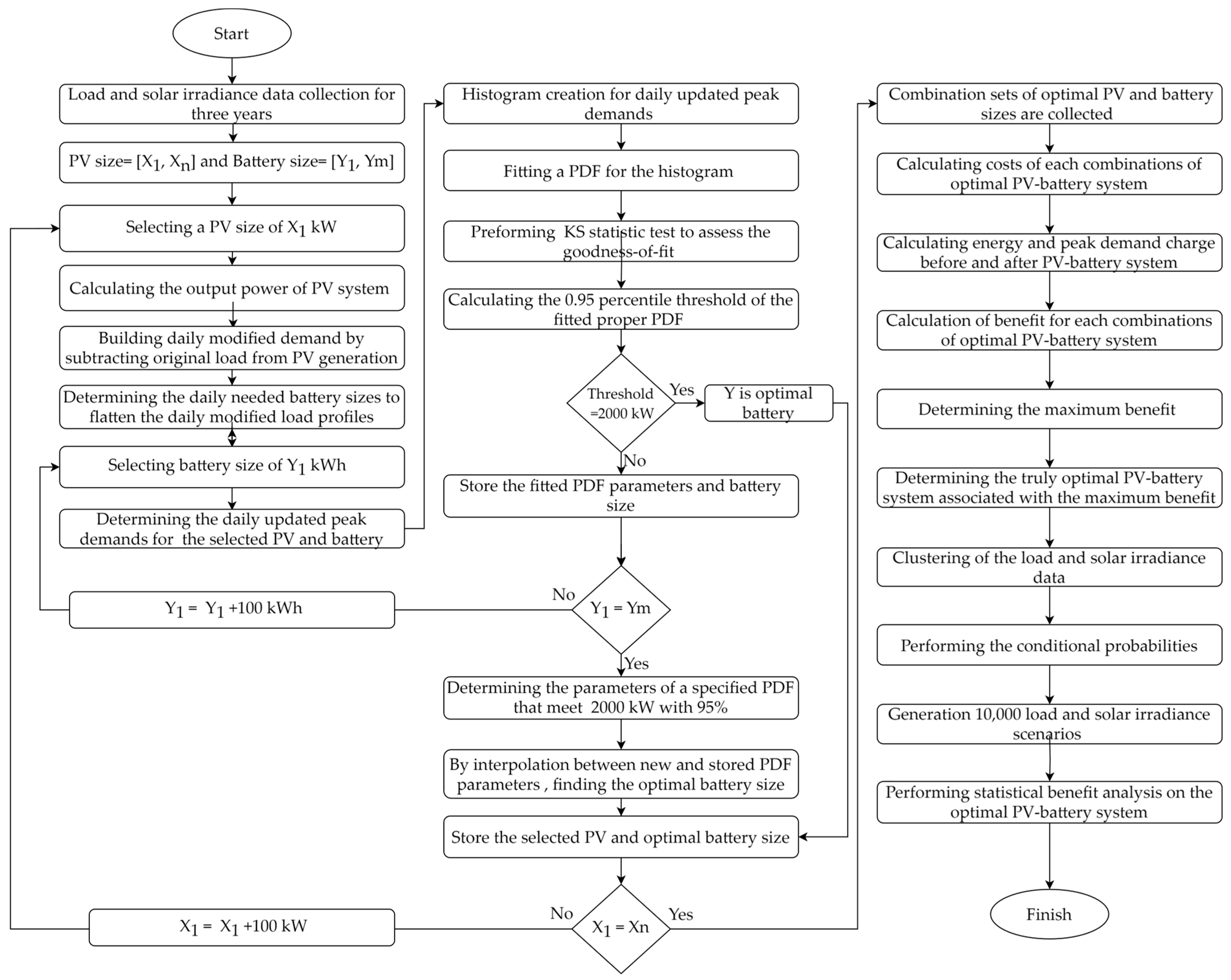
2.6. Statistical Analysis

This strategy was leveraged by fitting a proper PDF to the scaled histograms of the updated daily peaks. In this study, we used three well-known PDFs, Gamma, Log-normal, and Beta, where their shapes were similar to the derived daily peaks in PV–battery histograms. The Gamma distribution is useful in modeling variables that are always positive and have asymmetric distributions. The PDF of a Gamma distribution is given by [35]:

$$f(x)=\frac{{(\frac{x-\mu }{\beta })}^{\alpha -1}\exp (-\frac{x-\mu }{\beta })}{\beta \Gamma (\alpha )}$$

(5)

where $\alpha$, $\beta$, and $\mu$ are shape, scale, and location parameters, respectively, and $\Gamma (\alpha )$ is the Gamma function and can be expressed as follows [35]:

$$\Gamma (\alpha )={\displaystyle \underset{0}{\overset{\infty }{\int }}{t}^{\alpha -1}\exp (-t)dt}$$

(6)

The Beta distribution is a versatile statistical distribution used to model random variables, and the PDF of a Beta distribution is given by [36]:

$$f(x)=\frac{\Gamma (\alpha + \beta )}{\Gamma (\alpha )\Gamma (\beta )}{x}^{\alpha -1}{(1-x)}^{\beta -1}$$

(7)

where $\alpha$ and $\beta$ are shape and scale parameters for the Beta distribution.

The Log-normal distribution is suitable for modeling variables where the data are positively skewed and constrained to positive values, such as energy usage or peak demand levels. The PDF of a Log-normal distribution is [37]:

$$f(x)=\frac{1}{x\sigma \sqrt{2\pi }}\exp (-\frac{1}{2}{(\frac{\ln (x)-\mu }{\sigma })}^2)$$

(8)

where $\mu$ indicates the mean of data, and $\sigma$ represents the standard deviation. Besides, the Kolmogorov–Smirnov (KS) statistic test was utilized to evaluate the fitted PDFs for their accuracy in modeling the updated peak demands in this study. The KS test is particularly adept at assessing how well the selected PDFs conform to the empirical distribution of the updated peak demand data obtained from the system simulations. This test measures the largest difference between the empirical distribution of the observed peak demand data and the cumulative distribution functions (CDFs) of the theoretical models [38]. The distribution with the smallest KS statistic score and largest p-value (typically, a p-value larger than 0.05 is set) was considered the best fit for the data [39]. This means it has the smallest maximum deviation and, thus, most closely represents the behavior of the observed peak demands. After identifying the most suitable PDFs for various combinations of PV and battery sizes, we undertook the following steps to determine the optimal PV–battery system configuration:

• Selection of PV and battery sizes. We started by selecting a PV size of X₁ and calculating the updated daily peak demand across various battery sizes ranging from Y₁ to Y_m.
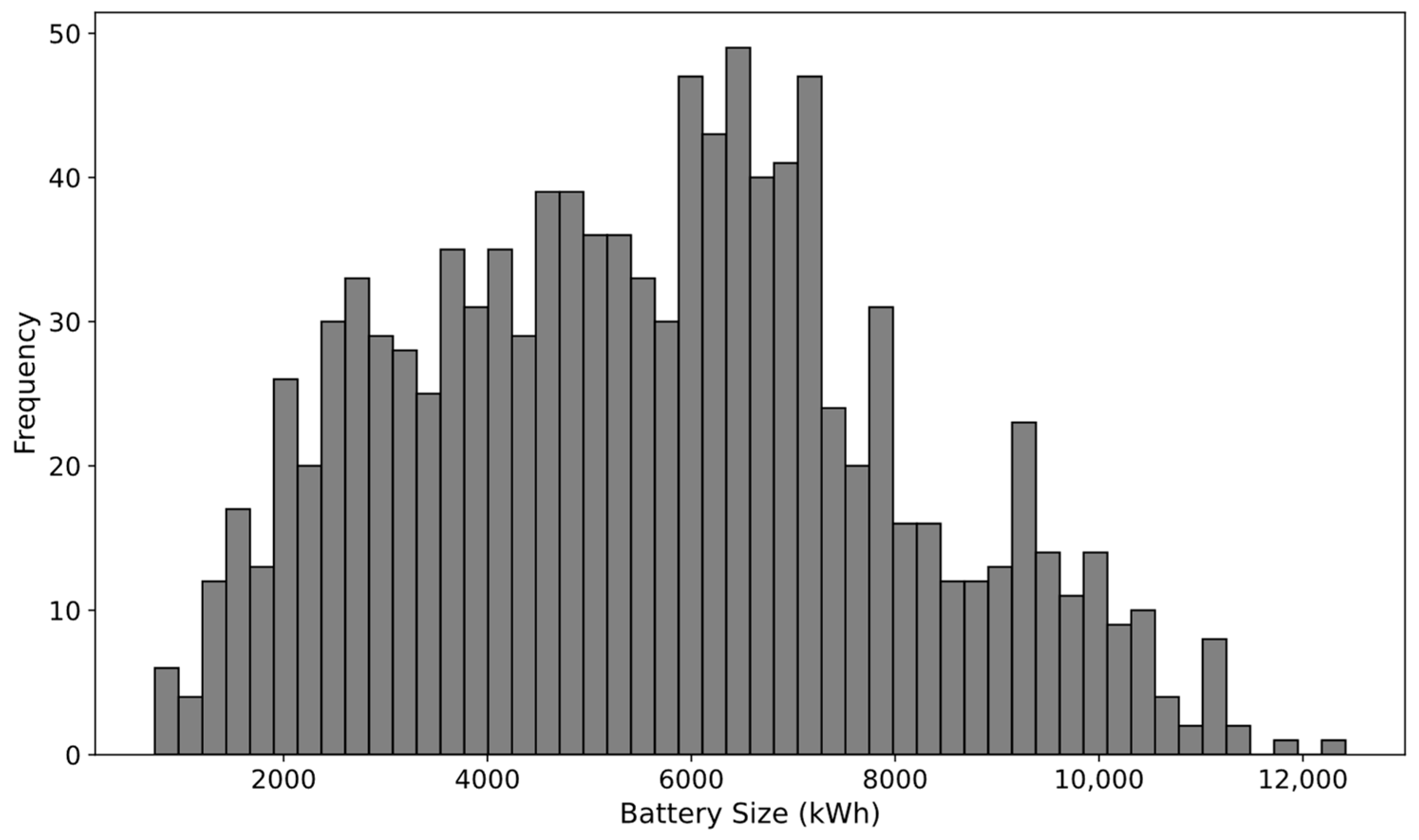
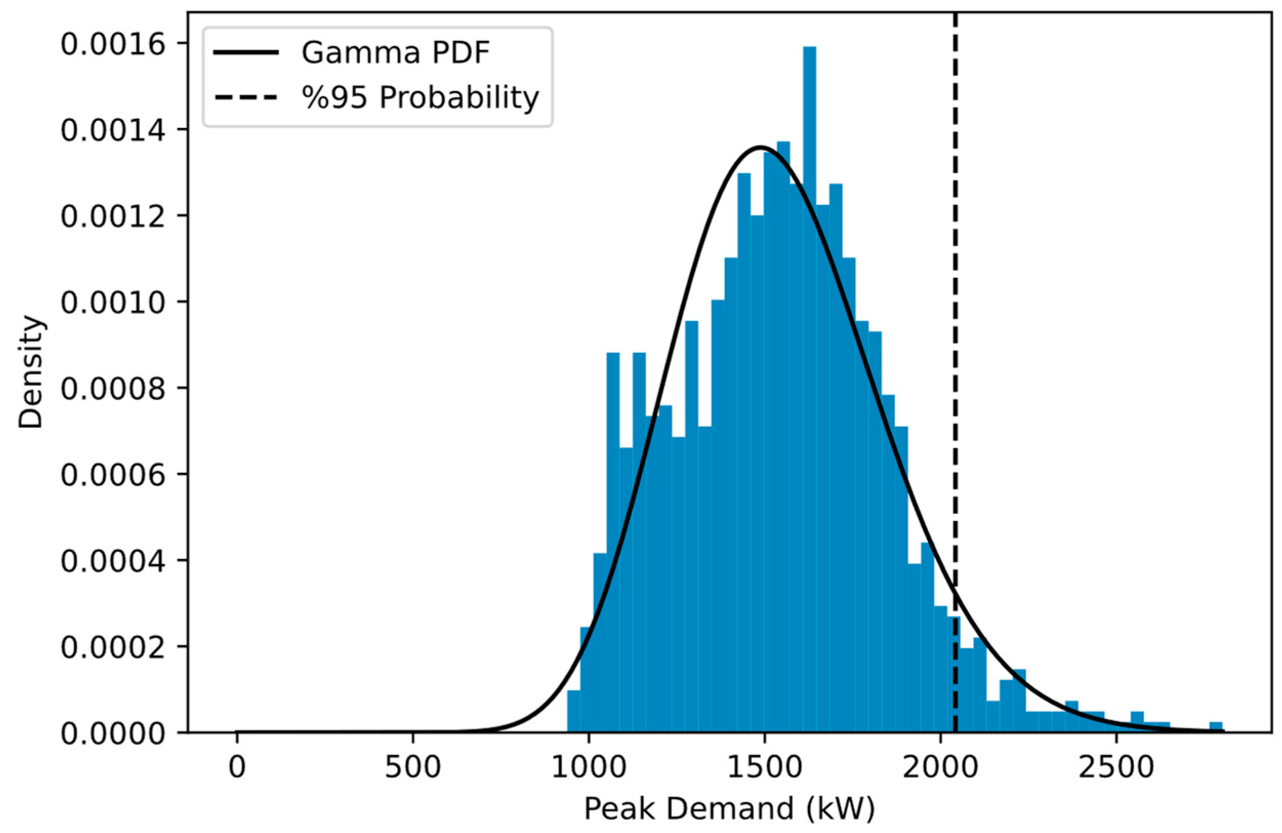
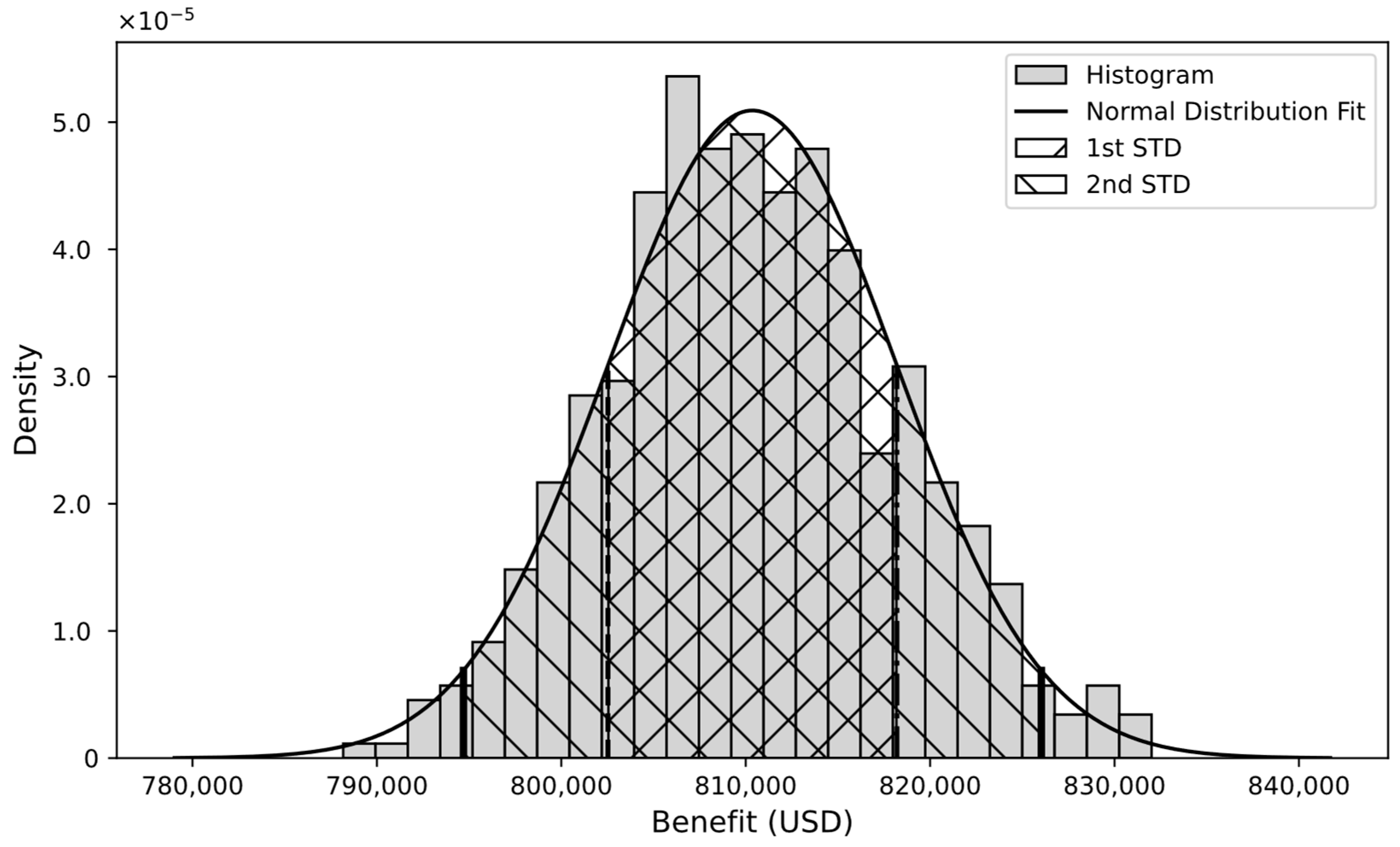
• Histogram creation and PDF fitting. For each PV–battery size, we generated scaled histograms of daily peak demands following PV–battery installation. These histograms were then fitted with appropriate PDFs, specifically chosen for their relevance, characterized by PDF parameters.
• Determining the 0.95 threshold. For each PDF, we calculated the threshold value that corresponds to the 95th percentile. Mathematically, this is represented as:

$$F^{-1}(P=0.95)$$

(9)

where $F^{-1}$ is the inverse of the CDF for the fitted PDF. This calculation yields multiple threshold values for each PV–battery combination.

4.

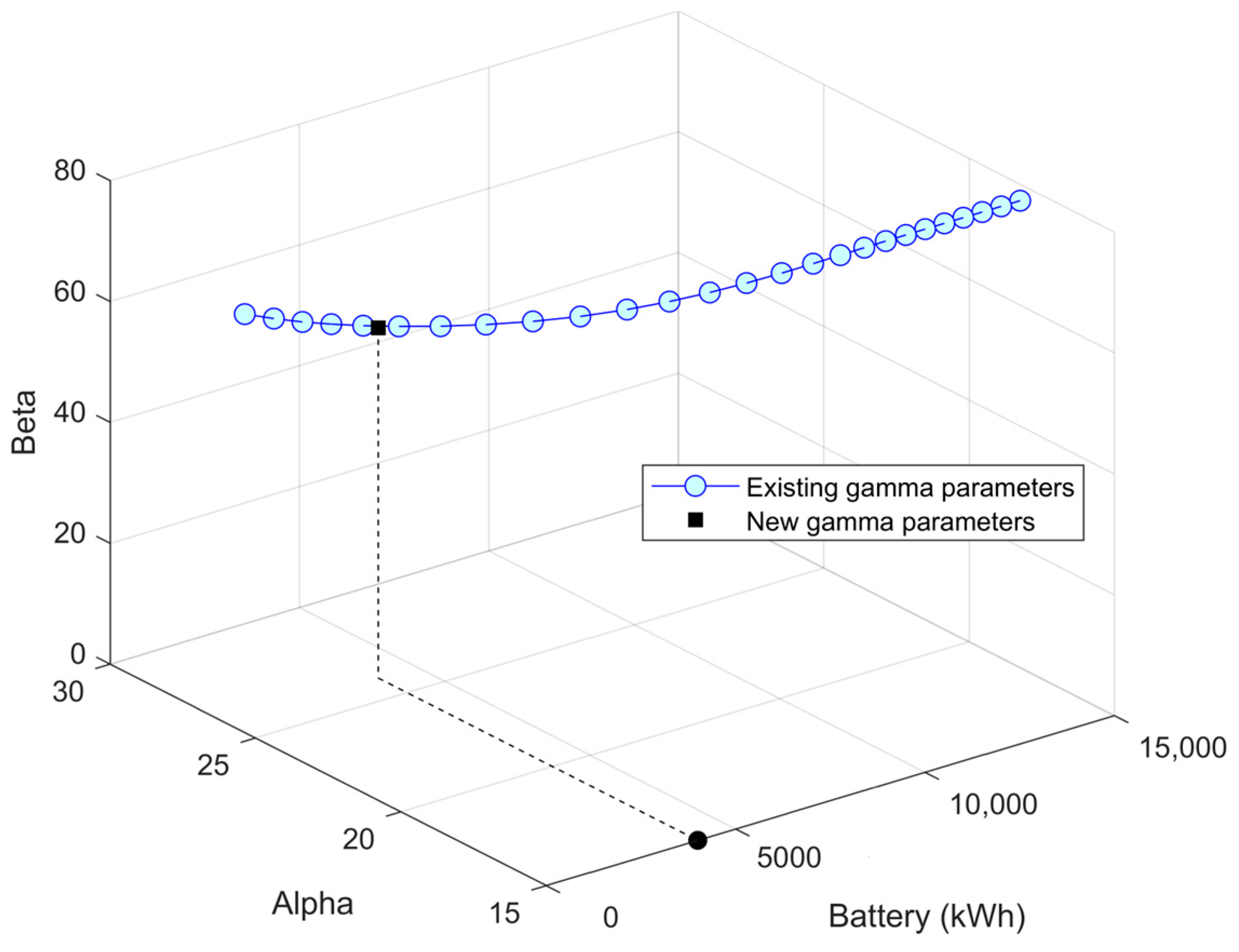
Optimal sizing criteria. The objective was to find the PV–battery size combination that meets a predetermined threshold of T kW with a 95% probability. If the desired threshold, T, aligns with the thresholds found in Equation (9), the corresponding battery size is considered optimal for the PV size of X₁. In cases where the desired threshold, T, did not align with the previously determined thresholds, we adjusted our approach and recalculated the parameters of a new PDF to match the desired threshold, T, with a 95% probability. This was achieved through the formula:

$$F(T, \mathrm{Parameters})=0.95$$

(10)

After recalibrating the new parameters of a new PDF to align with the T kW threshold at a 95% probability level, we used interpolation between the newly found parameters and those determined in step 3. This interpolation helped us identify the corresponding optimal battery size for these updated parameters.

5.

Optimal PV–battery system. By repeating all the aforementioned steps for a wide range of PV sizes, we eventually compiled an extensive set of optimal PV and battery combinations. Each of these combinations was capable of flattening 95% of the daily peaks up to a fixed threshold of T kW, which meets the technical requirement.

However, while these combinations technically satisfied the peak demand flattening criteria, the selection of the most suitable PV–battery system for actual implementation also requires a thorough economic analysis.

2.7. Economic Analysis

To determine the truly optimal PV–battery system for installation, it is essential to assess each determined PV–battery combination from an economic perspective. In this study, we rigorously evaluated the financial benefits of each PV–battery combination identified in our previous analyses. This economic evaluation for a PV size of X kW and battery size of Y kWh involves several key components, as follow:

2.7.1. Initial Investment Cost

We first assessed the initial capital investment required for each PV–battery combination. This included the costs of:

• PV installation [40]:

$$C_{pv}^{ini} = X·C_{pv}$$

(11)

Here, $C_{pv}^{ini}$ represents the total cost of the PV installation (USD), and $C_{pv}$ is the capital cost of PV panels in USD/kW.

• Inverter cost [41]:

$$C_{inv}^{ini} = X·{\eta }_{inv}·K·C_{inv}$$

(12)

where, $C_{inv}^{ini}$ is the total installation cost for the inverter (USD), $C_{inv}$ is the capital cost of the inverter in USD/kW, and K represents the oversized parameter of the invertor.

• Labor cost [42]:

$$C_{labor}^{ini} = X·C_{labor}$$

(13)

where, $C_{labor}^{ini}$ is the total initial human and labor cost (USD) and $C_{labor}$ is the cost of labor in USD/kW.

• Equipment costs [43]:

$$C_{eq}^{ini} = X·C_{eq}$$

(14)

where, $C_{eq}^{ini}$ is the total initial equipment cost (USD) and $C_{eq}$ is the capital cost of equipment in USD/kW.

• Overhead costs:

$$C_{over}^{ini} = X·C_{over}$$

(15)

where, $C_{over}^{ini}$ is the total initial overhead cost (USD) and $C_{over}$ is the cost of overhead in USD/kW.

• Battery cost:

Since the battery lifespan is typically shorter than the project lifetime, it is anticipated that the battery will require replacement during the project duration. Therefore, the initial cost of the first battery is as follows:

$$C_{bat}^{1,ini} = Y·C_{bat}^1$$

(16)

where, $C_{bat}^{1,ini}$ is the initial cost of the first battery (USD), and $C_{bat}^1$ is the capital cost of the first battery in USD/kWh. However, with the rapid advancement in battery technology, the cost for a replacement battery is expected to decline. Thus, the cost of the replacement battery can be expressed as follows [44]:

$$C_{bat}^{2,ini} = Y·C_{bat}^2$$

(17)

where, $C_{bat}^{2,ini}$ is the total initial cost of the replacement battery (USD), and $C_{bat}^2$ is the capital cost of the replacement battery in USD/kWh. Besides, the cost for the second battery must be adjusted to its present worth considering the expected decrease in cost and the time value of money. This is calculated using the formula for present worth, considering the discount rate of i and the period of M in which the replacement is needed [45]:

$$C_{bat}^{2,present} = C_{bat}^{2,ini}·\frac{1}{{(1+i)}^M}$$

(18)

where $C_{bat}^{2,present}$ represents the present worth of the replacement battery (USD). Accordingly, the total initial battery cost of $C_{bat}^{ini}$, accounting for both the first installation and the present worth of the replacement battery, is then given by:

$$C_{bat}^{ini} = C_{bat}^{2,present} + C_{bat}^1$$

(19)

Finally, considering the cost of the required transformers, $C_{trans}^{ini}$, for the PV–battery system, the total initial investment costs (TIIC) can be expressed as follows:

$$\mathrm{TIIC} = C_{pv}^{ini} + C_{inv}^{ini} + C_{labor}^{ini} + C_{eq}^{ini} + C_{over}^{ini} +C_{trans}^{ini}+C_{bat}^{ini}$$

(20)

2.7.2. Operation, Maintenance, and Insurance Costs

Once the PV–battery system is operational, there are ongoing costs that must be accounted for to ensure its continuous and efficient functionality. The annual operation costs typically cover monitoring and routine inspections. Maintenance costs include regular cleaning, repair, and replacement of components. Lastly, insurance is crucial for protecting the investment against risks, such as damage, theft, and other liabilities. The annual costs associated with the operation, maintenance, and insurance of the PV–battery system are as follows:

$$C_{O\&M}^{annual}=X·C_{O\&M}$$

(21)

where $C_{O\&M}^{annual}$ represents the annual costs of operation, maintenance, and insurance (USD), and $C_{O\&M}$ is the capital cost associated with them in USD/kW. Since these costs are incurred annually over the life of the system, N, its present worth can be calculated as follows [45]:

$$C_{O\&M}^{present}=C_{O\&M}^{annual}\left[\frac{1-{(1+i)}^{-N}}{i}\right]$$

(22)

2.7.3. Peak Demand and Energy Costs

An important component of the economic analysis is the peak demand charge, which represents the cost incurred by the highest level of demand recorded (measured in kW), typically within a month. The peak demand cost of $PD{C}_n$ for year n can be expressed as follows [46]:

$$PD{C}_n={\displaystyle \sum _{m=1}^{12}{P}_m^{\max }·C_{peak}}$$

(23)

where $P_m^{\max }$ is the peak demand of month m, and $C_{peak}$ represents the peak demand rate in USD/kW. Energy cost is the expense incurred for using electricity, determined by multiplying the quantity of electrical energy consumed by the rate charged by the electricity supplier. The energy cost of $E{C}_n$ for year n can be expressed as follows:

$$E{C}_n={\displaystyle \sum _{h=1}{P}_h·C_{energy}}$$

(24)

where $P_h$ is the hourly electricity consumption and $C_{energy}$ represents the energy rate in USD/kWh. To accurately compute the economic benefits of PV–battery installation, it is necessary to determine these costs before and after the implementation of the PV–battery system. Besides, these costs are annuities recurring at yearly intervals. Therefore, the present value of these charges over the system lifetime, N, must be calculated to evaluate the economic benefit effectively.

The present value of peak demand charge before installation, $PD{C}_{before PV-bat}^{present}$, is:

$$PD{C}_{Before PV-bat}^{present}={\displaystyle \sum _{n=1}^N\left(PD{C}_n·\left[\frac{1}{{(1+i)}^n}\right]\right)}$$

(25)

Similarly, the present value of peak demand charge after installation, $PD{C}_{After PV-bat}^{present}$, is:

$$PD{C}_{After PV-bat}^{present}={\displaystyle \sum _{n=1}^N\left({PDC}_n^{’}·\left[\frac{1}{{(1+i)}^n}\right]\right)}$$

(26)

where ${PDC}_n^{’}$ represents the yearly peak demand charge after PV–battery installation.

The present value of energy cost before PV–battery installation, $E{C}_{before PV-bat}^{present}$, is:

$$E{C}_{before PV-bat}^{present}={\displaystyle \sum _n^N\left(E{C}_n·\left[\frac{1}{{(1+i)}^n}\right]\right)}$$

(27)

Similarly, the present value of energy cost after PV–battery installation, $E{C}_{Aefore PV-bat}^{present}$, is:

$$E{C}_{Aefore PV-bat}^{present}={\displaystyle \sum _n^N}\left({EC}_n^{’}·\left[\frac{1}{{(1+i)}^n}\right]\right)$$

(28)

where ${EC}_n^{’}$ represents the yearly energy cost after PV–battery installation.

2.7.4. Economic Benefit

The economic benefit of installing a PV–battery system is a critical aspect of this study, encompassing the overall financial advantages gained over the system lifespan. The economic benefit of the PV–battery system installation is quantified by comparing the total costs incurred before and after the PV–battery installation and is calculated as follows:

$$\mathrm{Total} \mathrm{cost} \mathrm{before} \mathrm{PV-battery} \mathrm{installation}=E{C}_{before PV-bat}^{present} + PD{C}_{Before PV-bat}^{present}$$

(29)

$$\mathrm{Total} \mathrm{cost} \mathrm{after} \mathrm{PV-battery} \mathrm{installation}=\mathrm{TIIC} + C_{O\&M}^{present} + PD{C}_{After PV-bat}^{present} + E{C}_{Aefore PV-bat}^{present}$$

(30)

$$\mathrm{Benefit}=\mathrm{Total} \mathrm{cost} \mathrm{before} \mathrm{PV-battery} \mathrm{installation}-\mathrm{Total} \mathrm{cost} \mathrm{after} \mathrm{PV-battery} \mathrm{installation}$$

(31)

A positive economic benefit demonstrates that the PV–battery system is cost-effective. The savings on energy and peak demand charges outweigh the combined costs of installation, operation, and maintenance. We extended this economic evaluation across all optimal combinations of the PV–battery system that met a predetermined threshold of T kW with a 95% probability. This comprehensive analysis enabled the identification of the optimal PV–battery system configuration that maximized the utility benefit. Nonetheless, the inherent uncertainties within historical demand and solar irradiance data necessitate a rigorous validation of the robustness of the optimal PV–battery system under varied conditions. Variations in demand and irradiance are critical factors that could significantly influence the efficacy of the system. To consider these uncertainties and validate the resilience of the proposed solution, we employed an effective Monte Carlo simulation methodology. This simulation generates multiple scenarios, each representing distinct daily demand and solar irradiance conditions, thereby providing a holistic test of the model’s robustness.

2.8. Modified Monte Carlo Simulation

Monte Carlo simulation is a statistical technique that utilizes random sampling and probabilistic modeling for scenario analysis, decision-making, and predictive modeling. It operates by running a large number of simulations with random variables, thereby generating a wide range of possible outcomes and their probabilities [47]. However, in this study, the typical approach to Monte Carlo simulation requires modification due to the simultaneous consideration of two parameters: daily load and solar irradiance profiles. The goal is to generate multiple scenarios that accurately reflect the interdependence of solar irradiance and demand profiles throughout the year. A challenge in this methodology is the logical pairing of load and solar irradiance profiles to reflect realistic conditions. For instance, it is not methodologically sound to associate a high demand profile, typical of summer conditions, with a solar irradiance profile of winter. Such contradictions lead to skewed results and impair the reliability of the simulation. To address this, we have integrated a clustering technique to categorize similar load demands and solar irradiance profiles into distinct groups to effectively generate load and solar irradiance scenarios.

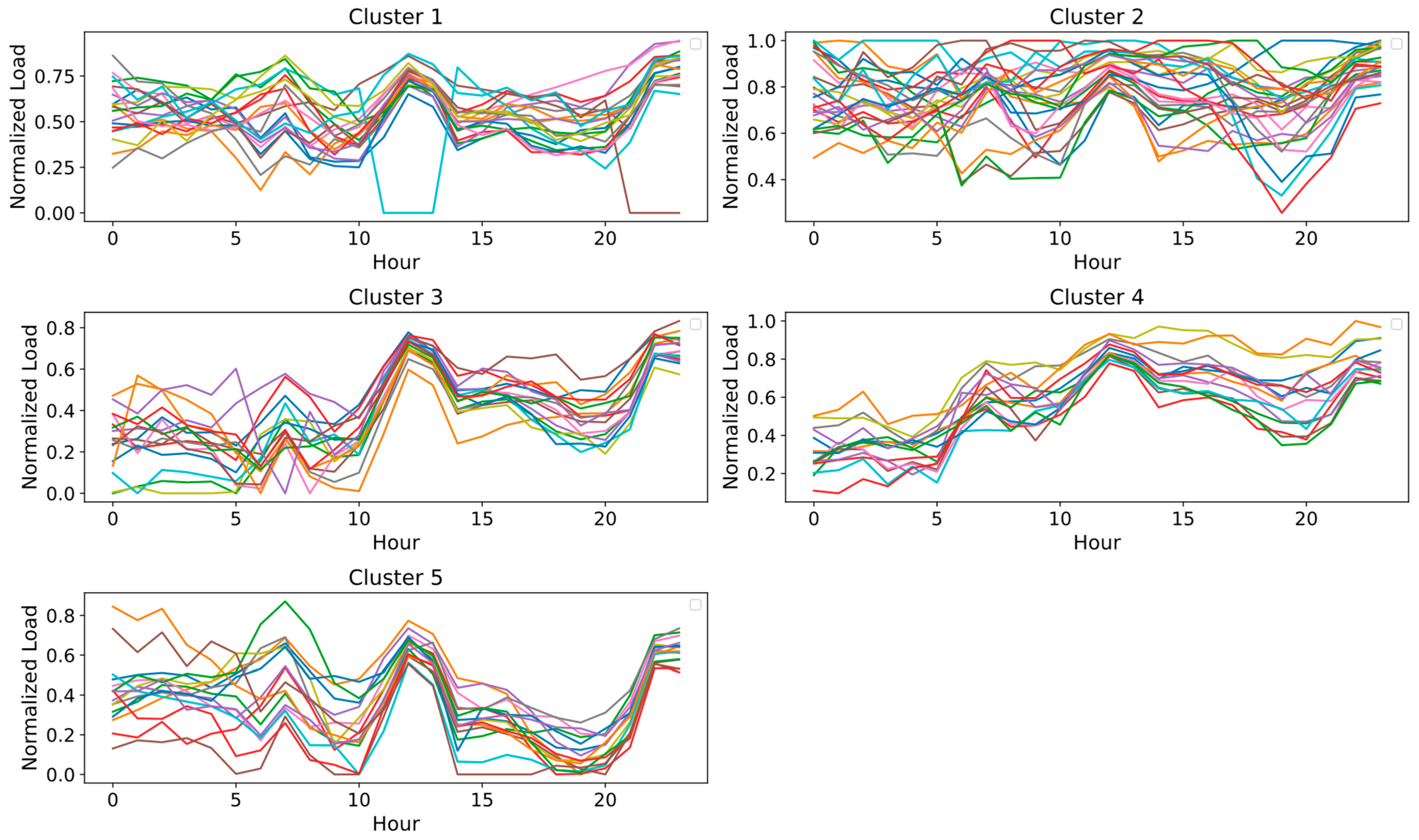
2.8.1. Time Series Clustering

The time series clustering involves grouping similar temporal data patterns into distinct clusters. To cluster the time series data of load demands and solar irradiance, we categorized three years of data on a monthly basis. Subsequently, within each month, daily time series for load and solar irradiance were clustered separately. In this study, we employed a structured approach to cluster time series data, involving the following steps [48]:

• Data preprocessing. The first step involved comprehensive data preparation. This includes cleaning the data to remove any inconsistencies or errors, addressing outliers, and ensuring that all data are correctly formatted. Subsequently, we normalized the data values to fall between 0 and 1. This standardization is crucial for comparability analysis. Then, we grouped the data monthly, aggregating three years of data for further analysis.
• Similarity measures. The objective of time series clustering is to categorize time series datasets into clusters, where datasets within each cluster exhibit maximum similarity among themselves and minimal similarity with datasets in other clusters. A similarity measure is crucial in quantifying the degree of resemblance between two time series datasets. In this study, we employed dynamic time warping (DTW), a technique that has demonstrated significant efficacy in assessing similarity, particularly in the energy management sector [49]. DTW compares each point of one time series with multiple points of another, finding the best alignment by minimizing the cumulative distance between these matched points. By allowing such flexibility in the alignment, DTW effectively captures the inherent patterns and shapes within the time series data, even when these occur at different rates or phases.
• Clustering algorithms. The next step was to employ an appropriate time series clustering algorithm. Time series clustering is a complex process, and validation of the time series clustering results is challenging. For this purpose, we utilized two distinct clustering algorithms, including K-means and self-organizing maps (SOM), ensuring a robust and thorough examination of the time series data, enhancing the reliability of the results. The K-means clustering method is a partitioning clustering algorithm that has shown effective performance in various power system clustering applications [50]. It is adept at managing non-Euclidean similarity measures, demonstrates resilience against outliers, and has lower computational complexity relative to other partitioning clustering algorithms, making it a suitable choice for this study [51]. Despite its advantages in time series clustering, it cannot autonomously determine the optimal number of clusters. On the other hand, SOM is an unsupervised neural network that can inherently determine the optimal number of clusters as part of its training process. SOM visualizes high-dimensional data in a low-dimensional map and preserves the topological and temporal structure of the data. This capability of SOM facilitates the identification of patterns and trends within complex time series datasets [52]. However, SOM requires a careful selection of the appropriate map size and learning parameters. This combination of partitioning and neural network-based clustering methods helped us analyze load demand and solar irradiance clustering. K-means identifies distinct clusters based on similarity measures, while SOM captures complex patterns and relationships within the data through neural network layers. By leveraging the strengths of both approaches, we can gain a comprehensive understanding of the underlying structures in the dataset.

K-means clustering aims to partition the data into K clusters, in which each data point belongs to the cluster with the nearest mean, serving as a prototype of the cluster. The K-means algorithm operates through the following iterative steps [51]:

• Initialization—The process began by randomly selecting k data points as the initial centroids of the clusters.
• Assignment step—In this phase, each data point in the dataset was assigned to the nearest centroid. The closeness was determined based on the DTW distance.
• Update step—The centroids of the clusters were then recalculated as the mean of all points assigned to each cluster.
• Convergence—These steps were repeated until the positions of the centroids stabilized, indicating that the clusters had converged and were no longer significantly changing.
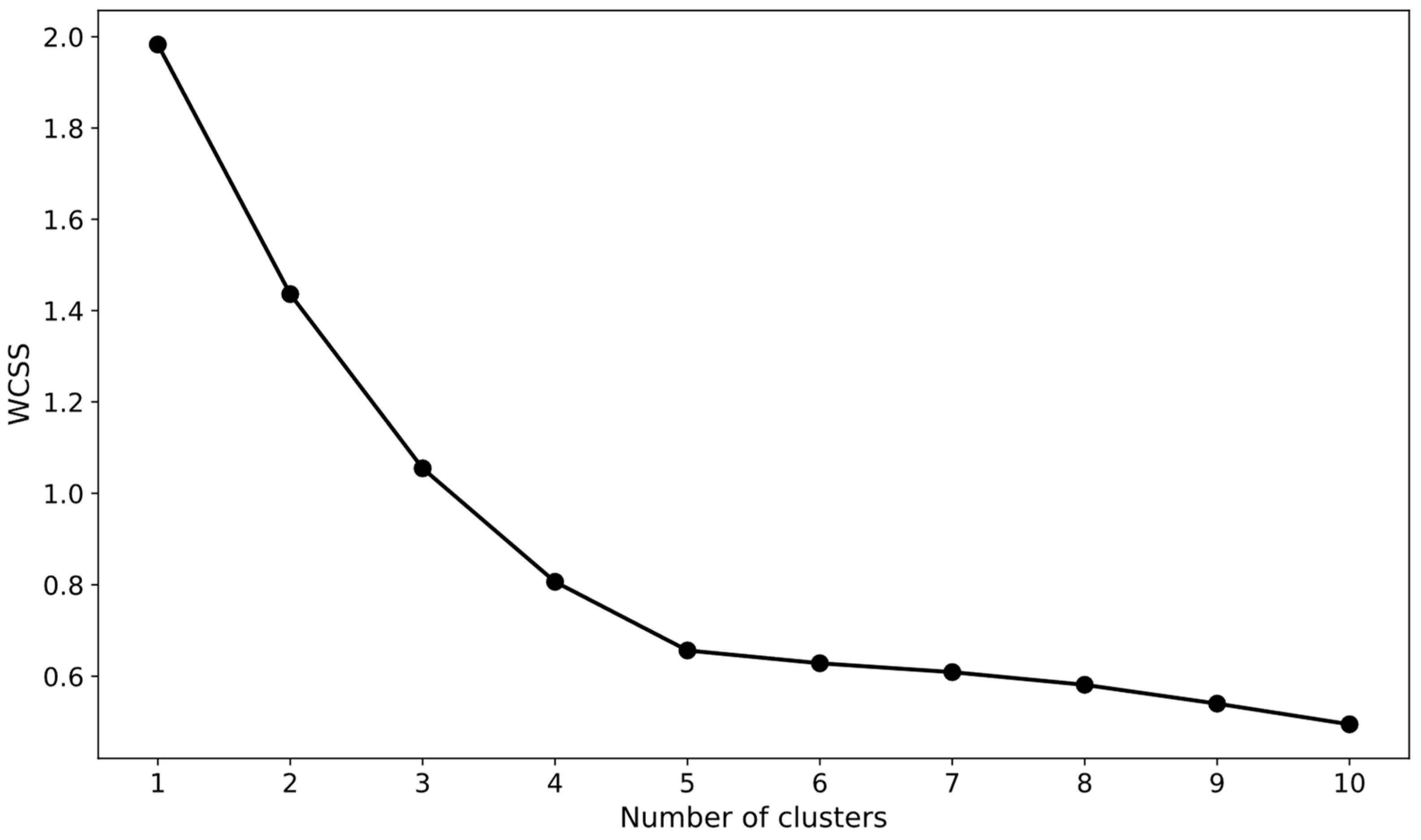
• Optimal number of clusters—Determining the optimal number of clusters is a critical aspect of the K-means algorithm. We employed the Elbow method to identify this number. To apply the Elbow method, we first executed the K-means algorithm over a range of K values, from 1 to a predefined maximum, then computed the Within-Cluster Sum of Squares (WCSS) for each K, and finally plotted these WCSS values against their cluster number. By observing the WCSS curve, we looked for a point where the rate of decrease in WCSS significantly slowed down, creating an elbow in the plot. The K value at this elbow point is considered the optimal number of clusters, as it indicates a trade-off between maximizing the number of clusters and minimizing WCSS [53].

SOM is a type of artificial neural network that is trained using unsupervised learning to produce a low-dimensional map. The methodology for applying SOM in this study is as follows [54]:

• Initialization—We started by initializing the SOM neural network with weight vectors, through random selection.
• Competitive learning—For each data point in our dataset, SOM identified the Best Matching Unit (BMU) by finding the neuron with the closest weight vector to the data point.
• Weight adjustment—The weights of the BMU and its neighbors within the network were adjusted to become more similar to the input data point, with the adjustment magnitude decreasing over time and distance from the BMU.
• Iterative process—This cycle of competitive learning and weight adjustment was repeated across numerous iterations, allowing the SOM to evolve and form a map that reflects the intrinsic structure of the data.
• Cluster visualization—The final output was a map where similar data points were clustered together.

Finally, we systematically compared the results obtained from both K-means and SOM clustering techniques. Then, the results were integrated into the modified Monte Carlo simulation to generate meaningful load and solar irradiance scenarios.

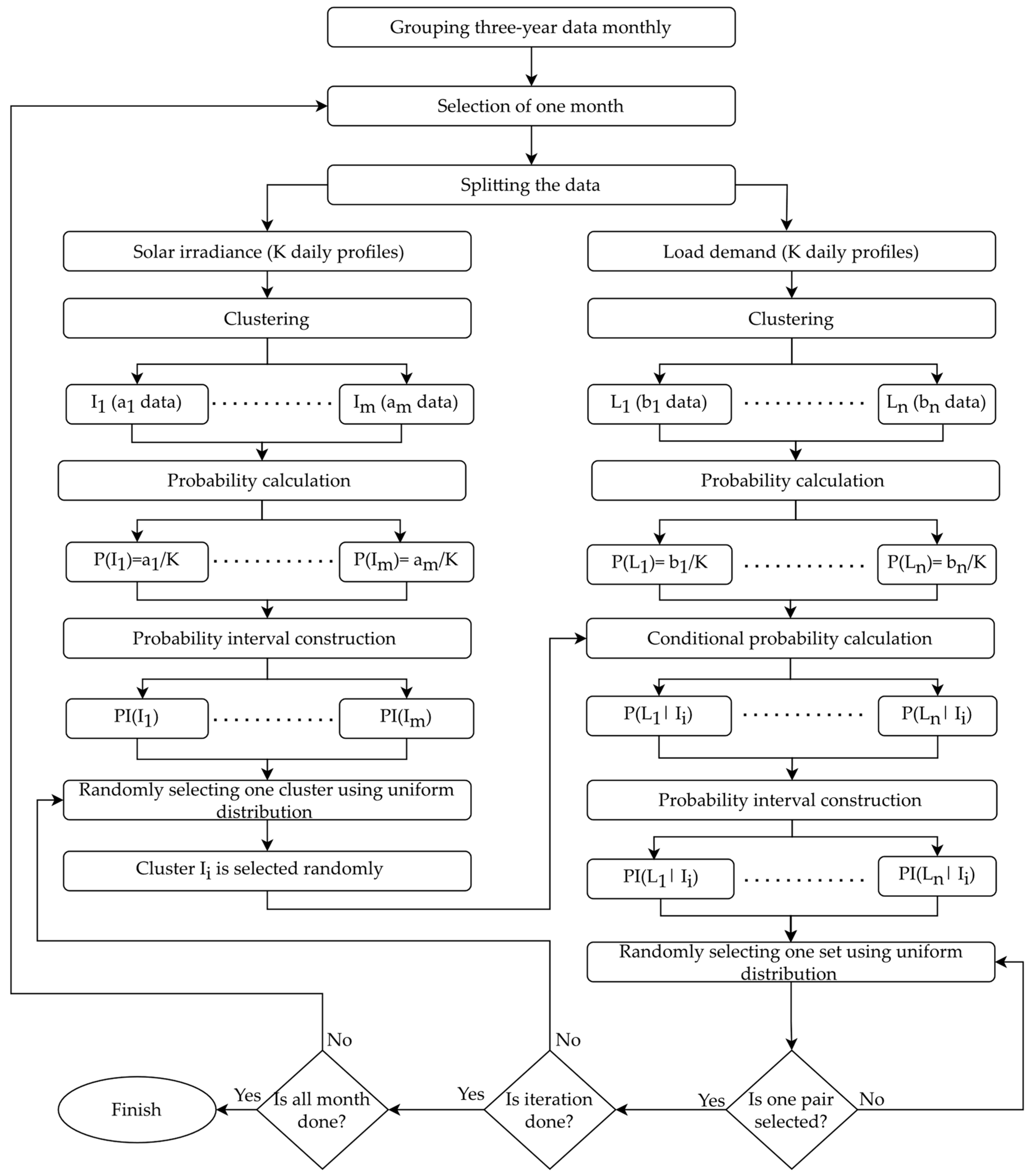
2.8.2. Modified Monte Carlo Simulation

After clustering the daily load and solar irradiance for each month, we implemented a modified Monte Carlo simulation to generate realistic scenarios. Assuming we have solar irradiance, clusters labeled set $\left\{I_1, I_2, I_3,\dots , I_m\right\}$, and load demand clusters labeled set $\left\{L_1, L_2, L_3,\dots , L_n\right\}$ for a month, the steps for a typical month were as follows:

• Assign probabilities to solar irradiance clusters. For each solar irradiance cluster $I_i$ (i = 1 to m), we calculated its probability as:

  $$P(I_i)=\frac{\mathrm{Number} \mathrm{of} \mathrm{data} \mathrm{within} \mathrm{cluster} I_{\mathrm{i}} }{\mathrm{Total} \mathrm{number} \mathrm{of} \mathrm{data} \mathrm{within} \mathrm{the} \mathrm{month}}$$

  (32)
• Establish probability intervals. This was carried out by sequentially adding the probabilities of the clusters. For the first cluster $I_1$, its probability interval, $PI(I_1)$ is:

  $$PI(I_1)=[0, P(I_1)]$$

  (33)

For the second cluster $I_2$, the interval is defined as:

$$PI(I_2)=(P(I_1), P(I_1)+P(I_2)$$

(34)

This continues for each cluster $I_m$, where:

$$PI(I_m)=(P(I_1)+P(I_2)+\dots +P(I_{m-1}), P(I_1)+P(I_2)+\dots +P(I_{m-1})+P(I_m)$$

(35)

3.

Random cluster selection for solar irradiance. A random number R within the range [0, 1] was selected uniformly, selecting the solar irradiance cluster $I_i$ for which the random number R falls within its probability interval.

4.

We determined the specific days that are included in the selected solar irradiance cluster.

5.

Match the days with load clusters. For each identified day in the solar irradiance cluster $I_i$, we found the corresponding days within the load demand clusters from $L_1$ to $L_n$.

6.

Calculate the conditional probability for load clusters. After selecting the solar irradiance cluster $I_i$, the probability of each load demand cluster conditioned on the selection of $I_i$ was calculated. The conditional probability was calculated as:

$$P(L_j|I_i)=\frac{P(L_j\cap I_i)}{P(I_i)}$$

(36)

7.

We established probability intervals for each conditional probability, as in step 2.

8.

We randomly selected a load cluster based on the conditional probability intervals.

9.

Final scenario selection. From the selected solar irradiance cluster $I_i$ and the randomly chosen load cluster $L$, a specific pair of solar irradiance and load demand profile was identified. If multiple profile pairs were available within the selected clusters, one pair was randomly selected. This random selection can be performed using a uniform distribution, ensuring each pair has an equal chance of being chosen.

All the steps to generate load demand and solar irradiance are demonstrated in Figure 5. These steps ensure that the final scenario chosen for each day accurately reflects the interdependencies between solar irradiance and load demand patterns, as dictated by the conditional probabilities. This approach enhances the realism and applicability of the scenarios generated for the Monte Carlo simulation, crucial for robust and insightful analysis.

3. Results

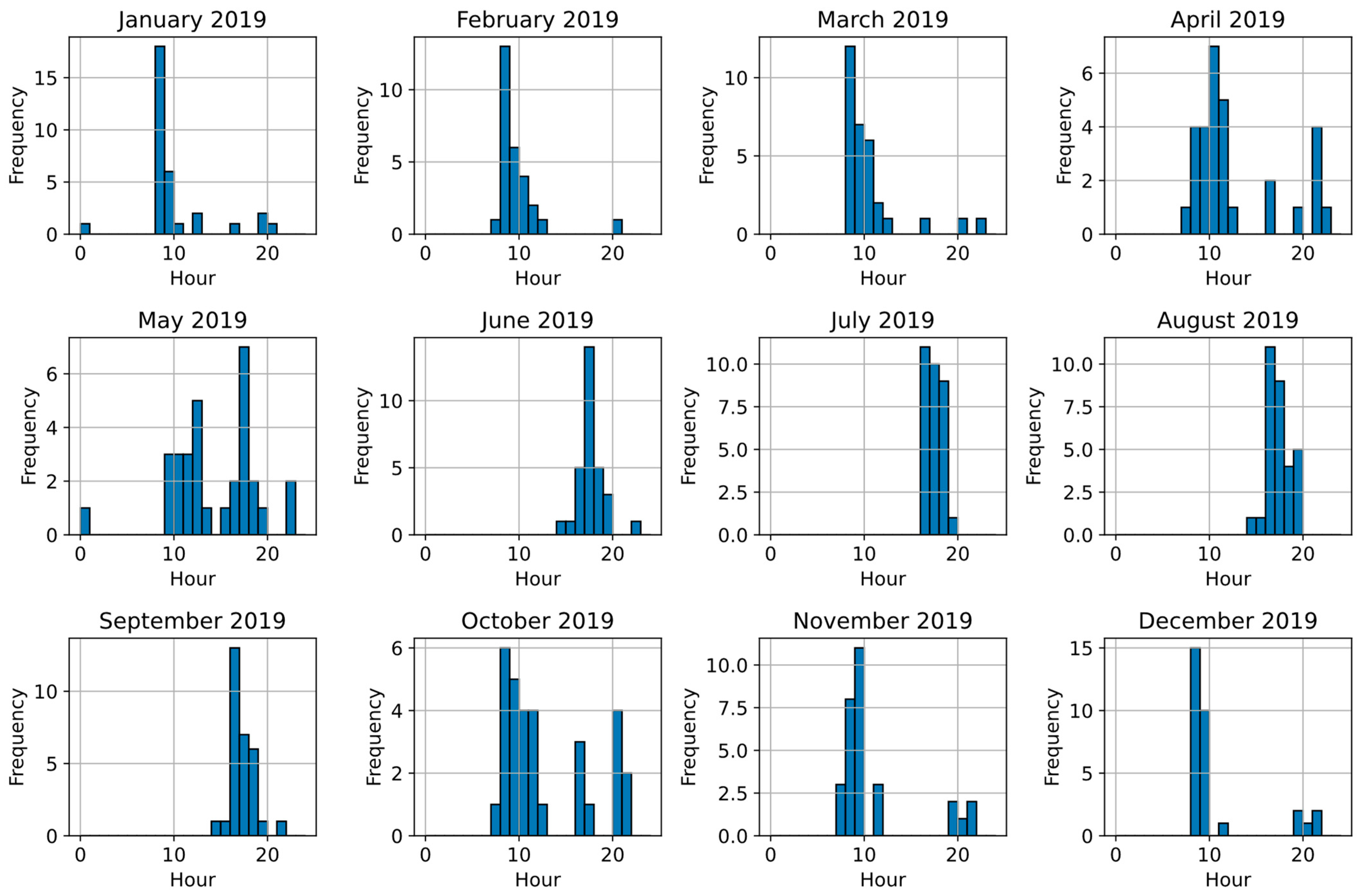
3.1. Data Analysis

A comprehensive analysis was conducted to investigate the occurrence of daily peak demand hours and their correlation with solar irradiance levels. For this purpose, the daily peak hours for each month were depicted and examined. The results of this analysis are presented in Figure 6. In the winter months, a significant trend was observed where the peak demand hours predominantly occurred during early morning times. Notably, these periods coincided with minimal solar irradiance, highlighting a critical gap in demand supply when relying solely on PV systems. Similarly, in the summer months of June, July, and August, peak demand hours were mostly observed in the late evening (18:00 to 20:00), when solar irradiance is not at its peak, despite it being higher during the noon hours throughout the year. These patterns across different months suggest that PV installations might not substantially contribute to peak demand reduction on most days of the year due to this misalignment with solar irradiance. Accordingly, battery storage can be a potential solution, capable of storing excess energy during off-peak hours or energy purchased from the grid, to be later utilized during peak demand periods. This strategic use of battery storage can potentially enhance the effectiveness of PV systems in peak demand reduction, highlighting its importance in overall energy management.

3.2. Battery Operation—Required Daily Battery Sizes

In this study, we considered PV system sizes ranging from X₁ = 200 kW to X₂ = 10,000 kW, paired with battery storage capacities from Y₁ = 200 kWh to Y_m = 10,000 kWh, incrementing in steps of 100. For each PV size, the modified load profile was calculated by subtracting the original load profiles from the PV generations. Then, for each of these modified profiles, the battery sizes needed to flatten the daily load curves were determined. For example, Figure 7 illustrates this for a 2000 kW PV system, showing a histogram of the required daily battery sizes that effectively flattened the load profiles for each day. The histogram has multiple peaks and is widespread, indicating significant variability in the required daily battery sizes. The variety in sizes likely reflects fluctuations in daily solar generation and load profiles. The distribution of sizes underscores the challenge of selecting a single, optimal battery size for a PV size of 2000 kW. For instance, while a large battery, such as one with a capacity of 12,000 kWh, could address peak demands on most days and effectively flatten the daily load profiles, it is not economically efficient due to its high cost. Conversely, a smaller battery might be more cost-effective but could lead to inadequate load flattening on days with higher energy demands.

3.3. Optimal PV–Battery System

Building upon the previous results of the required daily battery sizes for modified load profile flattening, this section examines optimal sizing for PV–battery systems. For each PV and battery size combination, we calculated the updated daily peak demands after PV–battery system integration. Then, the scaled histograms of the updated daily peaks for each combination of the PV–battery sizes were created. Next, three PDFs of Gamma, Log-normal, and Beta were fitted for each histogram. To assess the goodness-of-fit, a KS statistic test was performed on the fitted PDFs. The results revealed that the Gamma distribution fit the updated daily peak demands appropriately.

Table 2. KS statistic test results for the fitted PDFs for PV = 2000 kW and various batteries.

	Log-Normal		Gamma		Beta
Battery	KS_Statistic	p-Value	KS_Statistic	p-Value	KS_Statistic	p-Value
2000	0.041089	0.0480	0.031794	0.65124	0.08	0.005355
2500	0.03537	0.12579	0.029497	0.55618	0.11	0.027578
3000	0.040364	0.15470	0.026193	0.56416	0.09	0.005044
3500	0.026193	0.43233	0.053331	0.42345	0.12	0.04289
4000	0.062428	0.037	0.027589	0.65164	0.16	0.01455
4500	0.039343	0.06544	0.03461	0.32136	0.13	0.004353
5000	0.046593	0.01660	0.030778	0.32103	0.14	0.000539
5500	0.051666	0.00554	0.062428	0.27564	0.15	0.000127
6000	0.054413	0.00292	0.034076	0.24565	0.25	5.58 × 10−5

presents the results of the KS statistic test, comparing the fits of the Gamma, Log-normal, and Beta distributions to the updated daily peak demands for a PV size of 2000 kW across various battery sizes. The KS statistics and p-values indicate that the Gamma distribution consistently offered a better fit for the data compared to the Log-normal and Beta distributions. This is evident from the generally lower KS statistic values and higher p-values for the Gamma distribution across all battery sizes. For instance, at a battery size of 2000 kWh, the Gamma distribution had a KS statistic of 0.031794 and a p-value of 0.65124, which are considerably more favorable than those for the Log-normal and Beta distributions, suggesting a more accurate and reliable fit.

After identifying the Gamma distribution as the best-fitted PDF for the updated daily peak demands, the next step involved determining a 0.95 percent threshold. For each fitted Gamma PDF, we calculated the value corresponding to the 95th percentile, effectively establishing a threshold that represents the maximum peak level that the PV–battery system is expected to flatten on 95% of the days. For example, Figure 8 presents the fitted Gamma PDF for updated daily peaks with a PV size of 2000 kW and battery size of 3000 kWh. The Gamma distribution parameters were α = 26.805 and β = 57.668, with a threshold at 2041.996 kW, indicating only a 5% chance of exceeding this peak demand.

Then, for each combination of PV and battery, unique Gamma PDF parameters, including shape, scale, and thresholds, were derived. However, the utility desired peak demand threshold is 2000 kW with a 95% probability, indicating that the system should not exceed a 2000 kW peak demand more than 5% of the time. Since an exact 95% probability threshold of 2000 kW was not found among the calculated peak demand thresholds, we recalibrated a new Gamma distribution to meet this specific criterion, using the formula:

$$2000=F^{-1}(0.95, shape, scale)$$

(37)

Since the inverse CDF of the Gamma distribution is not available in closed form, numerical methods were employed for approximation. For instance, with a PV size of 2000 kW, the recalibrated shape and scale parameters were found to be 25.99 and 57.92, respectively. It is noteworthy that the recalibrated Gamma parameters aligned closely with the actual data-derived parameters. This proximity suggests that the recalibrated parameters and associated Gamma distribution are strongly representative of actual daily peak demand data. Figure 9 illustrates the shape and scale parameters of the fitted Gamma PDFs for a PV size of 2000 kW and various battery sizes. By aligning the new parameters on this plot, the corresponding optimal battery size was determined to be approximately 4000 kWh. As a result, a battery size of 4000 kWh has been identified as optimal for a PV system of 2000 kW, capable of flattening 95% of daily peak demands up to the desired threshold of 2000 kW. Accordingly, the proposed methodology performed well in determining the appropriate battery size to meet specific demands. Applying this method to a wide range of PV sizes, from 200 kW to 10,000 kW, the optimal battery size for each PV configuration can be determined.

Table 3. Optimal battery sizes for PV–battery systems to flatten 95% of the daily peak demands.

PV (kW)	500	1000	1200	1500	2000	2500	3000	3500	4000
Battery (kWh)	NAN	NAN	9200	4400	4000	3800	3600	3400	3300

presents the optimal battery sizes for PV–battery systems to flatten 95% of daily peak demands. For PV sizes between 500 kW and 1000 kW, optimal battery sizes were not defined, implying these PV systems may not have a battery solution that can meet the peak flattening criteria within the study parameters. As the PV system size increased to 1200 kW, a substantial battery capacity of 9200 kWh was required. This indicates a significant need for battery storage to effectively flatten peak demands for a relatively small PV size of 1200 kW. As the PV system size continued to increase, there was a gradual decrease in the required battery size. This trend suggests increasing efficiency in peak demand reduction with larger PV systems, requiring relatively smaller batteries.

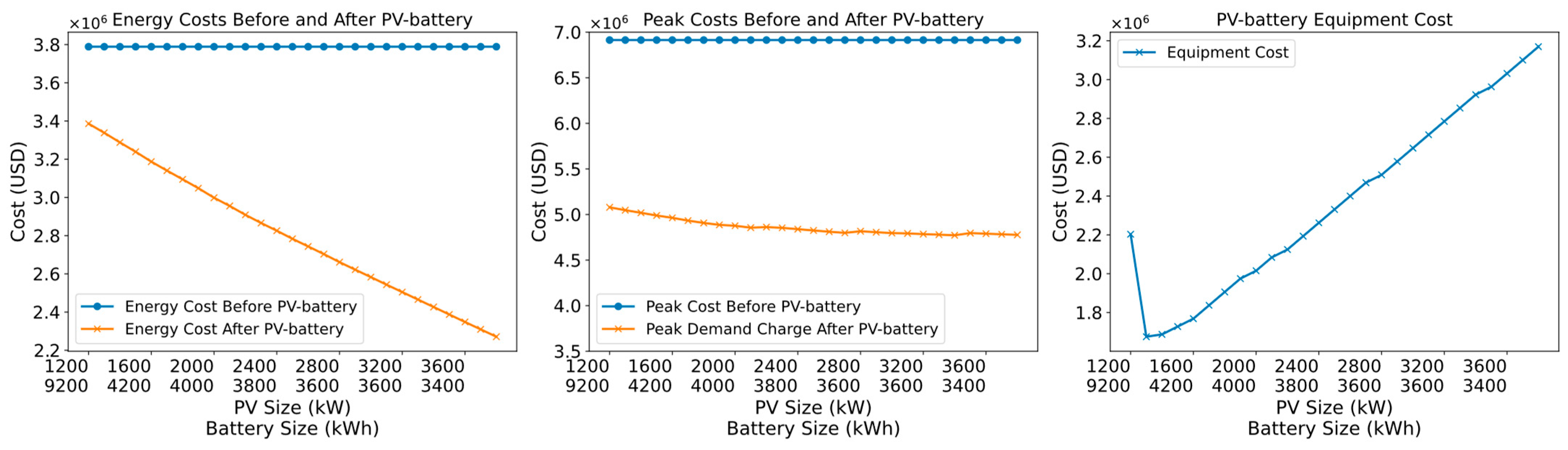
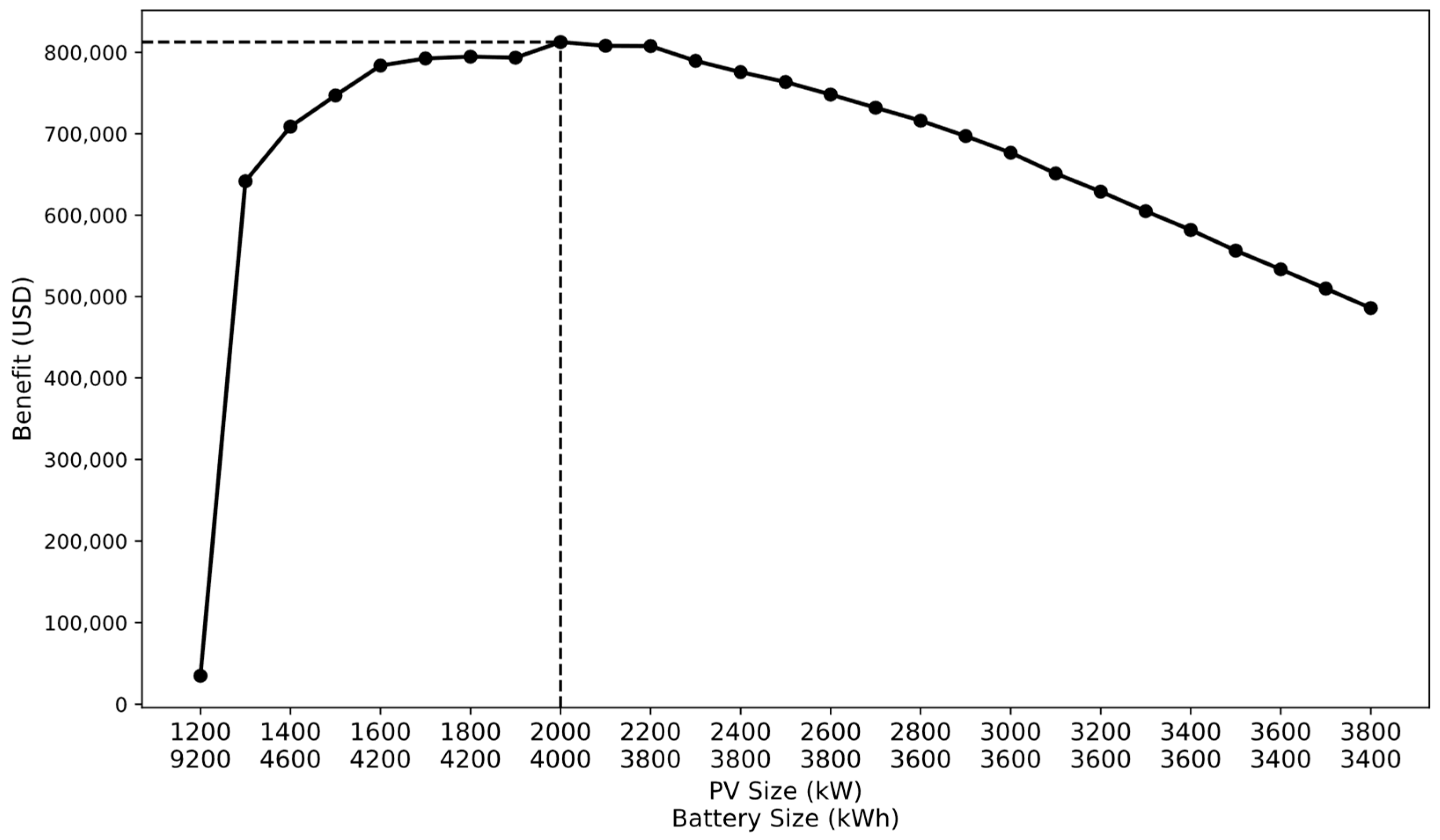
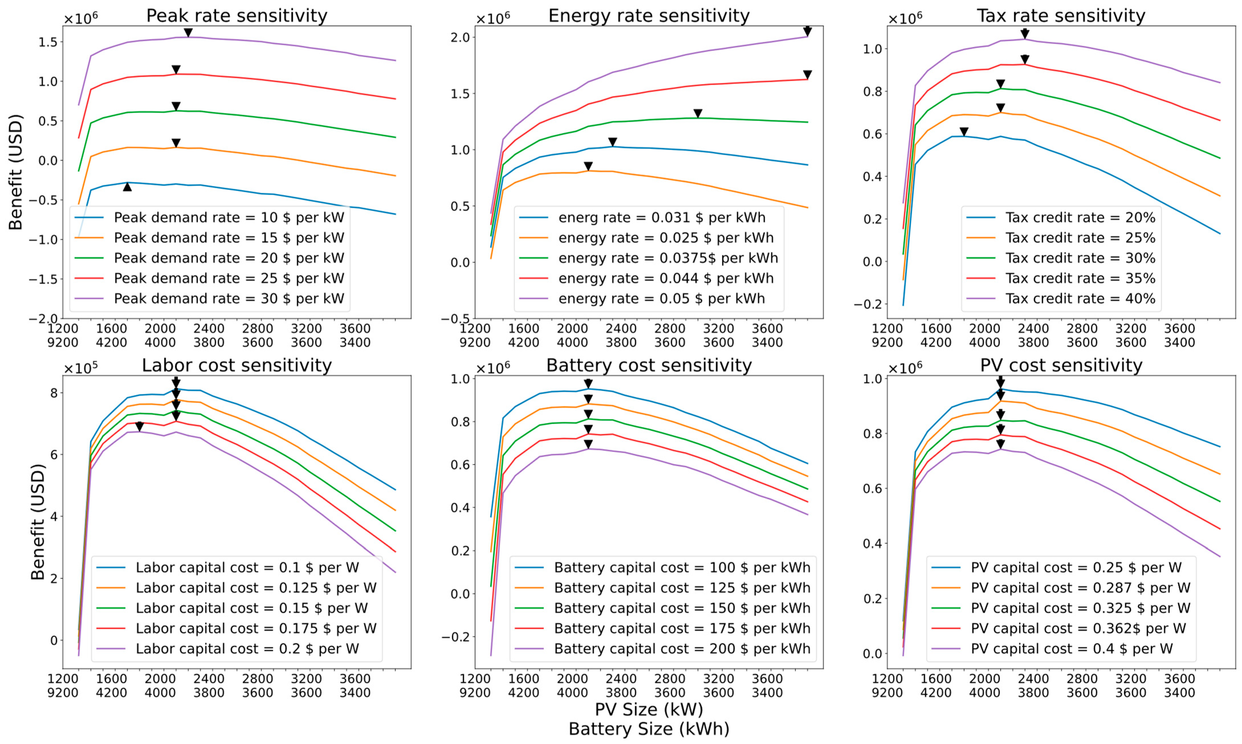
3.4. Financial Analysis

The proposed methodology provided a wide range of PV–battery configurations capable of effectively flattening 95% of the daily peak loads up to a threshold of 2000 kW. While technical optimization is pivotal, the economic viability of each configuration is equally essential. To this end, we computed a financial analysis for all identified optimal PV–battery combinations. This analysis for each combination was calculated by grouping three years of data on a monthly basis. For example, for January, we obtained three sets of load demand and solar irradiance data for 2019, 2020, and 2021. Within each month, we determined the average peak demand charges and average energy costs. We then combined them all into 1 year and calculated the benefit over 20 years. This detailed financial analysis for all combinations of optimal PV–battery sizes is illustrated in Figure 10. As the size of the PV system increased, the energy cost decreased. This is because larger PV systems have a greater capacity to reduce energy costs during operation. It should be noted that the contribution of the battery to reducing energy costs is limited, because rather than generating energy, batteries are primarily used to shift energy. Notably, the peak demand charge exhibited minimal variation across different PV–battery sizes. This consistency can be attributed to the fact that all optimal PV–battery configurations effectively flattened 95% of the daily load profiles, resulting in a consistent impact on the peak demand cost reduction. This minor discrepancy can be ascribed to the statistical fitting of the histograms into Gamma PDFs, which may not be ideally fitted. Additionally, the equipment cost exhibited a gradual increase. Despite the reduction in battery size as the PV size increased, the overall increase in PV size outweighed the decrease in battery size, resulting in a net rise in equipment costs. In particular, the equipment cost for a PV size of 1200 kW and a battery size of 9200 kWh was relatively high due to the elevated costs associated with large batteries. However, the subsequent reduction in battery size led to a notable drop in equipment costs.

Furthermore, the financial benefits for each PV–battery combination were computed and depicted in Figure 11. The PV–battery size that yielded the maximum utility benefit was considered as the most desirable system. Notably, a PV system with a size of 2000 kW with a 4000 kWh battery emerged as the most economically advantageous, yielding a maximum benefit of USD 812,648 over the project lifetime. This optimal benefit was identified as providing the greatest economic return for utilities.

Table 4. Economic analysis of the optimal PV–battery system (PV = 2000 kW and battery = 4000 kWh).

	Before PV–Battery	PV Only	After PV–Battery
Equipment cost (USD)	0	1,638,688	2,015,246
Energy cost (USD)	3,788,907	3,036,927	3,023,569
Peak demand charge (USD)	6,913,926	6,472,805	4,901,679
Benefit (USD)	0	−445,587	812,648

provides detailed economic information for the optimal PV–battery system. The total peak demand cost without the PV–battery system was almost twice the energy cost, thereby highlighting the substantial influence of peak demand charges on the overall utility costs. Upon the installation of a PV only, there was a notable decrease in energy costs by 19.8%, demonstrating the effectiveness of a PV-only system in reducing energy costs. However, the peak demand costs had a relatively modest reduction of only 6%, underscoring that while PV installations significantly contributed to energy cost savings, their impact on peak demand reduction was comparatively limited. The economic assessment of the PV-only system presented a less advantageous outcome. The high costs associated with the installation, maintenance, operation, and insurance of the PV system outweighed the savings costs, leading to a negative benefit for utilities. This highlights a critical limitation of relying solely on PV systems. In contrast, the integration of batteries with PV systems demonstrated a significant improvement in peak demand costs, with a reduction of up to 29%. This substantial decrease indicates the battery’s capability to effectively flatten daily peak demands. Although the addition of batteries incurred an extra energy cost of USD 25,155 due to losses inherent in battery operation, the overall peak demand charge savings were sufficient to offset these additional expenses. This resulted in a positive benefit of USD 812,648 over the project lifetime for utilities. Accordingly, the combined PV–battery system not only reduced the peak demand charges effectively but also provided a positive financial benefit for utilities.

The proposed statistical method successfully determined the optimal PV–battery system that provides a financial benefit for utilities. However, the obtained results were based on baseline economic parameters. Accordingly, a sensitivity analysis was conducted to rigorously evaluate the robustness and resilience of the proposed statistical system under varying economic conditions. This analysis helps to understand the potential impacts of fluctuations in energy costs, peak demand charges, and tax credits on the optimal PV battery systems. To undertake this sensitivity analysis, we systematically varied the assumptions related to energy costs, peak demand charges, capital costs of PV and battery systems, labor costs, and tax credit rates from their baseline values. The baseline scenario was based on an energy cost of USD 0.025/kWh, a peak demand charge of USD 22/kW, a PV capital cost of USD 0.35/kW, an initial battery cost of USD 150/kWh, a labor cost of USD 0.1, and tax credits at 30%. We adjusted the parameters for the sensitivity analysis with various values to assess their impact on the financial benefit of the PV–battery system. The results of this sensitivity analysis, which demonstrated how each economic parameter influenced the financial benefit of the PV–battery system, are depicted in Figure 12. Each subplot illustrates the impact of varying a single economic parameter while holding others constant. Additionally, the black triangles indicate the maximum benefit for each scenario. It was observed that the peak demand rate, energy rate, and tax credit rate had a direct relationship with financial benefits. In other words, as these rates increased, the maximum benefit also increased. Conversely, the capital costs of the labor, PV panels, and batteries exhibited an inverse relationship with the benefits. Although a high peak demand rate significantly enhanced the benefit, it did not markedly influence optimal PV–battery system sizes. This was attributed to the relatively equal contribution of all PV–battery combinations to flatten the daily peak demands. Consequently, with other parameters remaining constant, the peak demand rate had a minimal impact on selecting the optimal PV–battery system. Further, a peak demand rate of USD 10/kW did not provide positive financial benefits, thus making it uneconomical.

However, the energy rate influenced both the benefit and optimal PV–battery selection. Since battery installations do not contribute to energy reduction, larger PV sizes can yield more energy savings, resulting in increased financial benefits for utilities. With other economic parameters held constant, the increase in energy savings provided by larger PV systems outweighed the installation costs of PV–battery systems. Notably, for energy rates higher than 0.0375 USD/kWh, the impact on decision-making was significant, with larger PV sizes offering substantial energy savings. Tax credits affected the PV–battery installation costs, with higher tax credit rates leading to more cost savings and higher benefits. Additionally, higher tax credits resulted in larger PV–battery systems compared to lower tax credit rates, leading to larger optimal PV–battery configurations for higher tax credit rates.

Conversely, higher capital costs for labor, PV panels, and batteries led to decreased financial benefits, without significantly affecting the selection of optimal system sizes. The analysis revealed that as these costs increased from their baseline values, the financial benefits for various PV–battery configurations declined in a relatively uniform manner. This uniform reduction ensured that the choice of optimal systems remained consistent, highlighting the resilience of the optimal system size selection against fluctuations in capital cost rates. It should be noted that there were two distinct maximum benefit points on the peak rate and labor cost sensitivity curves, corresponding to the peak rate of USD 10/kW and labor cost of USD 0.2/kW. Despite these differences, the variations in maximum benefit values, when compared with other rates within the same plots, were slight.

This sensitivity analysis revealed that the proposed statistical methodology was influenced by the economic parameters of the system. Although peak demand, labor, battery, and PV panel rates altered the financial benefits, they had a minimal impact on selecting the optimal PV–battery system. This underscores the resilience and robustness of the proposed statistical model against these parameters. However, energy rates and tax credits significantly impacted the decision on selecting the optimal PV–battery size, highlighting the critical role of these economic parameters. This insight is crucial for utilities, emphasizing the need to consider these economic parameters when planning and implementing PV–battery systems.

In addition, to account for the inherent variability in load demand and solar irradiance, we employed a modified Monte Carlo simulation to rigorously test the performance of the optimal PV–battery system under diverse conditions.

3.5. Modified Monte Carlo Simulation

To categorize similar load and solar irradiance data into distinct clusters, we segmented three years of data by month. For instance, January data comprised 93 daily load profiles for both demand and solar irradiance, spanning across 3 years. These data points were normalized between zero and one for effective clustering. We employed K-means and SOM clustering algorithms to group each month’s data. The K-means algorithm was applied with varying cluster numbers, and for each, the WCSS was calculated. To create Elbow curves, we plotted the WCSS against various numbers of clusters to determine the optimal number of clusters. For example, Figure 13 shows the Elbow curve associated with the January load demand profile clustering. The reduction in WCSS from 1 to 5 clusters was relatively gradual. After 5 clusters, the decreases continued, but they were less pronounced. Considering these values, the optimal number of clusters could be around 5 clusters. By repeating this process for other months, the clusters were obtained for load demand and solar irradiance.

Since clustering is a complex process and determining the optimal number of clusters is challenging, the SOM technique was employed to validate these findings and offer deeper insights. Utilizing SOM with key parameters, such as a sigma of 0.01 and a learning rate of 0.5 over 1000 iterations, the SOM effectively identified similar data profiles. The process revealed distinct clusters within the data, as the SOM neuron grid self-organized based on the inherent similarities in load and solar irradiance profiles. This self-organization was evident in the final SOM grid, which visually represented the data points’ topological relationships, demonstrating clear patterns and groupings within the load and irradiance profiles. For example, the results of the January load profile are depicted in Figure 14. The number of clusters identified was 5, aligning with the findings from the K-means analysis, thereby confirming the success of the clustering process. These 5 distinct clusters demonstrated varying patterns in energy consumption, reflecting different energy usage behaviors. Notably, one of the load demand profiles within cluster 1 exhibited a relatively different pattern between hours 11 to 13 and 21 to 23, differing from other profiles during these particular hours. Despite these differences, the SOM algorithm grouped this load profile into cluster 1 instead of isolating it into a new single cluster. This decision can be attributed to the SOM overall pattern recognition approach, focusing on general daily energy usage trends rather than specific differences at certain hours. Furthermore, SOM clustering logic aims to avoid overfitting by not creating particular clusters for minor variations, ensuring a robust and generalizable grouping of load profiles. It should be noted that we employed clustering primarily to enhance the effectiveness of the Monte Carlo simulation. Consequently, a thorough exploration of the clustering patterns, which would require an extensive analysis including detailed consumer types and environmental information, is beyond the scope of this study.

After clustering the monthly load demand and solar irradiance data, we applied the established modified Monte Carlo simulation to generate 10,000 daily load and solar irradiance scenarios for each month. These were then aggregated into annual sequences, yielding 10,000 yearly datasets. For the 20-year benefit analysis, we randomly selected 20 distinct daily load and solar irradiance pairs per iteration, ensuring no repetition in the selection process. This procedure was repeated 500 times, creating 500 unique samples of 20-year benefit calculations. Accordingly, the benefit analysis for the optimal system, considering PV sizes of 2000 kW and a battery size of 4000 kW, was conducted under various ranges of demand and solar irradiance scenarios. The results of this comprehensive evaluation are depicted as histograms in Figure 15. The histogram analysis indicated that the average benefit over a 20-year period for the optimal PV–battery systems was USD 810,364. This central value suggests that, on average, the integration of the PV–battery system is expected to yield substantial financial benefits over the long term. Besides, the standard deviation of USD 7834.234 indicated a consistent performance of the PV–battery systems in terms of financial returns. The benefit histogram was fitted by a normal distribution with obtained mean and standard deviation. The first standard deviation range was between USD 802,529.82 and USD 818,198.28. This indicates that approximately 68% of the benefit values are expected to fall within this range, suggesting a high likelihood of achieving favorable financial outcomes close to the mean. Similarly, the second standard deviation extended the range to between USD 794,695.59 and USD 826,032.49. This wider range encompasses about 95% of the potential benefit outcomes, indicating that even when accounting for greater variability, the vast majority of benefits remained within an acceptable benefit range. The alignment of these values around the central mean suggests that significant deviations from the expected average are relatively uncommon. These statistical insights, derived from the benefit data, provide a robust foundation for anticipating the financial performance of the optimal PV–battery systems over a 20-year period. The concentration of data within the first and second standard deviations reinforces the reliability and stability of these systems as a financially viable solution in the long-term planning.

While the proposed statistical methodology successfully determined the optimal size of the PV–battery system by flattening 95% of the daily load demand and providing financial benefits for the utility, it is limited to those residential, commercial, and industrial customers, and utilities, who pay for electricity peak demand and are connected to primary power suppliers to meet the highest 5 percent of daily demand peaks that are not flattened. Additionally, the proposed methodology in this study, while initially based on economic parameters specific to a municipal utility in Kansas, can be applied to any utilities connected to the grid that incur peak demand charges. By adjusting the input parameters, such as solar irradiance levels, electricity rates, and installation costs, the model can be applied to other states or countries with distinct economic and environmental conditions.

4. Conclusions

This study addressed the significance of the peak demand reduction in optimizing grid-connected PV–battery systems. Considering that utility companies often incur energy and peak demand costs, PV installations should reduce energy and peak demand charges. The results revealed that PV installation alone reduced energy costs significantly, but its contribution to peak demand reduction was relatively low, leading to a negative benefit for utilities. Accordingly, battery storage was used to shift energy from off-peak to peak hours to mitigate the peak demands. Recognizing the importance of peak demand reduction, a novel statistical method was proposed to determine the optimal PV–battery system that can effectively flatten 95% of daily load profiles up to a threshold of 2000 kW, while accommodating the risk of not meeting the highest 5% of daily peak demands. Through a systematic and efficient search process, we identified optimal combinations of PV and battery sizes that meet these criteria. Based on economic analysis, the most cost-effective system for the utility company was a 2000 kW PV system with a battery of 4000 kWh, providing a benefit of USD 812,648 over 20 years. Moreover, the robustness of the optimal PV–battery system was rigorously tested against 10,000 diverse solar irradiance and load demand profiles. This was achieved by integrating time series clustering and applying conditional probabilities to effectively consider the interdependence between solar irradiance and demand profiles, using a modified Monte Carlo approach. However, this study is primarily applicable to utility companies connected to the grid and incurring peak demand charges. Future research is recommended in several areas:

• Integrating electric vehicles into the grid—enhancing grid adaptability to manage the stochastic load and energy contributions from electric vehicles. This initiative aims to optimize financial benefits and energy efficiency through the development of dynamic charging strategies and vehicle-to-grid technologies.
• Examining the influence of various grid topology and related constraints. A deeper exploration of how grid configurations and limitations affect the deployment and performance of PV–battery systems will refine the accuracy of the proposed methodology. It will enable the model to account for physical and regulatory constraints, thereby improving the feasibility and reliability of the system.
• Extending the methodology to include other renewable energy sources. By incorporating technologies, such as wind turbines, into a hybrid system, the framework can provide a more comprehensive analysis of renewable energy potentials. This holistic approach will facilitate the development of optimized, multi-faceted energy solutions that better meet the needs of utilities and consumers, while also promoting a more sustainable energy mix.
• Refining the methodology to determine the desired demand threshold. Tailoring the model to align with specific utility company requirements and operational capacities will enhance its practical relevance and effectiveness. Customizing the methodology in this way ensures that the proposed solutions are not only theoretically sound but also practically implementable, leading to more efficient energy management strategies.
• Investigating the integration of emerging photovoltaic technologies. Incorporating advanced solar technologies, such as dye-sensitized and perovskite solar cells, could pave the way for leveraging cutting-edge innovations in solar energy, potentially transforming the economic landscape of solar power by reducing costs and increasing efficiency.

References

- Betancourt Schwarz, M.; Veyron, M.; Clausse, M. Impact of Flexibility Implementation on the Control of a Solar District Heating System. Solar 2023, 4, 1–14. [Google Scholar] [CrossRef]
- Banibaqash, A.; Hunaiti, Z.; Abbod, M. Assessing the Potential of Qatari House Roofs for Solar Panel Installations: A Feasibility Survey. Solar 2023, 3, 650–662. [Google Scholar] [CrossRef]
- Chen, S.; Liu, N.; Xu, F.; Wei, G. Challenges and Strategies Toward Future Stable Perovskite Photovoltaics. Sol. RRL 2023, 7, 2300479. [Google Scholar] [CrossRef]
- Liu, N.; Wang, L.; Xu, F.; Wu, J.; Song, T.; Chen, Q. Recent Progress in Developing Monolithic Perovskite/Si Tandem Solar Cells. Front. Chem. 2020, 8, 603375. [Google Scholar] [CrossRef] [PubMed]
- Khan, F.; Alshahrani, T.; Fareed, I.; Kim, J.H. A Comprehensive Degradation Assessment of Silicon Photovoltaic Modules Installed on a Concrete Base under Hot and Low-Humidity Environments: Building Applications. Sustain. Energy Technol. Assess. 2022, 52, 102314. [Google Scholar] [CrossRef]
- Ali, A.; Volatier, M.; Darnon, M. Optimal Sizing and Assessment of Standalone Photovoltaic Systems for Community Health Centers in Mali. Solar 2023, 3, 522–543. [Google Scholar] [CrossRef]
- Nematirad, R.; Pahwa, A.; Natarajan, B.; Wu, H. Optimal Sizing of Photovoltaic-Battery System for Peak Demand Reduction Using Statistical Models. Front. Energy Res. 2023, 11, 1297356. [Google Scholar] [CrossRef]
- Kim, E.; Jamal, H.; Jeon, I.; Khan, F.; Chun, S.; Kim, J.H. Functionality of 1-Butyl-2,3-Dimethylimidazolium Bromide (BMI-Br) as a Solid Plasticizer in PEO-Based Polymer Electrolyte for Highly Reliable Lithium Metal Batteries. Adv. Energy Mater. 2023, 13, 2301674. [Google Scholar] [CrossRef]
- Agajie, T.F.; Ali, A.; Fopah-Lele, A.; Amoussou, I.; Khan, B.; Velasco, C.L.R.; Tanyi, E. A Comprehensive Review on Techno-Economic Analysis and Optimal Sizing of Hybrid Renewable Energy Sources with Energy Storage Systems. Energies 2023, 16, 642. [Google Scholar] [CrossRef]
- Owosuhi, A.; Hamam, Y.; Munda, J. Maximizing the Integration of a Battery Energy Storage System–Photovoltaic Distributed Generation for Power System Harmonic Reduction: An Overview. Energies 2023, 16, 2549. [Google Scholar] [CrossRef]
- Vossos, V.; Garbesi, K.; Shen, H. Energy Savings from Direct-DC in U.S. Residential Buildings. Energy Build. 2014, 68, 223–231. [Google Scholar] [CrossRef]
- Beck, T.; Kondziella, H.; Huard, G.; Bruckner, T. Assessing the Influence of the Temporal Resolution of Electrical Load and PV Generation Profiles on Self-Consumption and Sizing of PV-Battery Systems. Appl. Energy 2016, 173, 331–342. [Google Scholar] [CrossRef]
- Tervo, E.; Agbim, K.; DeAngelis, F.; Hernandez, J.; Kim, H.K.; Odukomaiya, A. An Economic Analysis of Residential Photovoltaic Systems with Lithium Ion Battery Storage in the United States. Renew. Sustain. Energy Rev. 2018, 94, 1057–1066. [Google Scholar] [CrossRef]
- Bendato, I.; Bonfiglio, A.; Brignone, M.; Delfino, F.; Pampararo, F.; Procopio, R.; Rossi, M. Design Criteria for the Optimal Sizing of Integrated Photovoltaic-Storage Systems. Energy 2018, 149, 505–515. [Google Scholar] [CrossRef]
- Belboul, Z.; Toual, B.; Kouzou, A.; Mokrani, L.; Bensalem, A.; Kennel, R.; Abdelrahem, M. Multiobjective Optimization of a Hybrid PV/Wind/Battery/Diesel Generator System Integrated in Microgrid: A Case Study in Djelfa, Algeria. Energies 2022, 15, 3579. [Google Scholar] [CrossRef]
- Mukhopadhyay, B.; Das, D. Multi-Objective Dynamic and Static Reconfiguration with Optimized Allocation of PV-DG and Battery Energy Storage System. Renew. Sustain. Energy Rev. 2020, 124, 109777. [Google Scholar] [CrossRef]
- Shivam, K.; Tzou, J.-C.; Wu, S.-C. A Multi-Objective Predictive Energy Management Strategy for Residential Grid-Connected PV-Battery Hybrid Systems Based on Machine Learning Technique. Energy Convers. Manag. 2021, 237, 114103. [Google Scholar] [CrossRef]
- Zhi, Y.; Yang, X. Scenario-Based Multi-Objective Optimization Strategy for Rural PV-Battery Systems. Appl. Energy 2023, 345, 121314. [Google Scholar] [CrossRef]
- Song, Z.; Guan, X.; Cheng, M. Multi-Objective Optimization Strategy for Home Energy Management System Including PV and Battery Energy Storage. Energy Rep. 2022, 8, 5396–5411. [Google Scholar] [CrossRef]
- Park, H. A Stochastic Planning Model for Battery Energy Storage Systems Coupled with Utility-Scale Solar Photovoltaics. Energies 2021, 14, 1244. [Google Scholar] [CrossRef]
- Javidsharifi, M.; Pourroshanfekr Arabani, H.; Kerekes, T.; Sera, D.; Guerrero, J.M. Stochastic Optimal Strategy for Power Management in Interconnected Multi-Microgrid Systems. Electronics 2022, 11, 1424. [Google Scholar] [CrossRef]
- Guo, E.; He, B.; Zhang, J. Effects of Photovoltaic Panel Type on Optimum Sizing of an Electrical Energy Storage System Using a Stochastic Optimization Approach. J. Energy Storage 2023, 72, 108581. [Google Scholar] [CrossRef]
- Ntube, N.; Li, H. Stochastic Multi-Objective Optimal Sizing of Battery Energy Storage System for a Residential Home. J. Energy Storage 2023, 59, 106403. [Google Scholar] [CrossRef]
- Zheng, Z.; Li, X.; Pan, J.; Luo, X. A Multi-Year Two-Stage Stochastic Programming Model for Optimal Design and Operation of Residential Photovoltaic-Battery Systems. Energy Build. 2021, 239, 110835. [Google Scholar] [CrossRef]
- Rong, S.; Zhao, Y.; Wang, Y.; Chen, J.; Guan, W.; Cui, J.; Liu, Y. Information Gap Decision Theory-Based Stochastic Optimization for Smart Microgrids with Multiple Transformers. Appl. Sci. 2023, 13, 9305. [Google Scholar] [CrossRef]
- Chaerani, D.; Shuib, A.; Perdana, T.; Irmansyah, A.Z. Systematic Literature Review on Robust Optimization in Solving Sustainable Development Goals (SDGs) Problems during the COVID-19 Pandemic. Sustainability 2023, 15, 5654. [Google Scholar] [CrossRef]
- Bakhtvar, M.; Al-Hinai, A. Robust Operation of Hybrid Solar–Wind Power Plant with Battery Energy Storage System. Energies 2021, 14, 3781. [Google Scholar] [CrossRef]
- Aghamohamadi, M.; Mahmoudi, A.; Haque, M.H. Two-Stage Robust Sizing and Operation Co-Optimization for Residential PV–Battery Systems Considering the Uncertainty of PV Generation and Load. IEEE Trans. Ind. Inform. 2021, 17, 1005–1017. [Google Scholar] [CrossRef]
- Coppitters, D.; De Paepe, W.; Contino, F. Robust Design Optimization and Stochastic Performance Analysis of a Grid-Connected Photovoltaic System with Battery Storage and Hydrogen Storage. Energy 2020, 213, 118798. [Google Scholar] [CrossRef]
- Nematirad, R.; Ardehali, M.M.; Khorsandi, A.; Mahmoudian, A. Optimization of Residential Demand Response Program Cost with Consideration for Occupants Thermal Comfort and Privacy. IEEE Access 2024, 12, 15194–15207. [Google Scholar] [CrossRef]
- Nematirad, R.; Pahwa, A. Solar Radiation Forecasting Using Artificial Neural Networks Considering Feature Selection. In Proceedings of the 2022 IEEE Kansas Power and Energy Conference (KPEC), Manhattan, KS, USA, 25–26 April 2022; pp. 1–4. [Google Scholar]
- Mellit, A.; Massi Pavan, A.; Ogliari, E.; Leva, S.; Lughi, V. Advanced Methods for Photovoltaic Output Power Forecasting: A Review. Appl. Sci. 2020, 10, 487. [Google Scholar] [CrossRef]
- Kaufhold, E.; Meyer, J.; Myrzik, J.; Schegner, P. Harmonic Stability Assessment of Commercially Available Single-Phase Photovoltaic Inverters Considering Operating-Point Dependencies. Solar 2023, 3, 473–486. [Google Scholar] [CrossRef]
- Li, R.; Huang, S.; Dou, H. Dynamic Risk Assessment of Landslide Hazard for Large-Scale Photovoltaic Power Plants under Extreme Rainfall Conditions. Water 2023, 15, 2832. [Google Scholar] [CrossRef]
- De Figueiredo, F.A.P.; Dias, C.F.; de Lima, E.R.; Fraidenraich, G. Capacity Bounds for Dense Massive MIMO in a Line-of-Sight Propagation Environment. Sensors 2020, 20, 520. [Google Scholar] [CrossRef] [PubMed]
- Althubyani, F.A.; Abd El-Bar, A.M.T.; Fawzy, M.A.; Gemeay, A.M. A New 3-Parameter Bounded Beta Distribution: Properties, Estimation, and Applications. Axioms 2022, 11, 504. [Google Scholar] [CrossRef]
- Valvo, P.S. A Bimodal Lognormal Distribution Model for the Prediction of COVID-19 Deaths. Appl. Sci. 2020, 10, 8500. [Google Scholar] [CrossRef]
- Upreti, D.; Pignatti, S.; Pascucci, S.; Tolomio, M.; Li, Z.; Huang, W.; Casa, R. A Comparison of Moment-Independent and Variance-Based Global Sensitivity Analysis Approaches for Wheat Yield Estimation with the Aquacrop-OS Model. Agronomy 2020, 10, 607. [Google Scholar] [CrossRef]
- Kyeong, S.; Kim, D.; Shin, J. Can System Log Data Enhance the Performance of Credit Scoring?—Evidence from an Internet Bank in Korea. Sustainability 2021, 14, 130. [Google Scholar] [CrossRef]
- Dehwah, A.H.A.; Asif, M.; Budaiwi, I.M.; Alshibani, A. Techno-Economic Assessment of Rooftop PV Systems in Residential Buildings in Hot–Humid Climates. Sustainability 2020, 12, 10060. [Google Scholar] [CrossRef]
- Hazim, H.I.; Baharin, K.A.; Gan, C.K.; Sabry, A.H.; Humaidi, A.J. Review on Optimization Techniques of PV/Inverter Ratio for Grid-Tie PV Systems. Appl. Sci. 2023, 13, 3155. [Google Scholar] [CrossRef]
- Raza, F.; Tamoor, M.; Miran, S.; Arif, W.; Kiren, T.; Amjad, W.; Hussain, M.I.; Lee, G.-H. The Socio-Economic Impact of Using Photovoltaic (PV) Energy for High-Efficiency Irrigation Systems: A Case Study. Energies 2022, 15, 1198. [Google Scholar] [CrossRef]
- Shepovalova, O.; Izmailov, A.; Lobachevsky, Y.; Dorokhov, A. High-Efficiency Photovoltaic Equipment for Agriculture Power Supply. Agriculture 2023, 13, 1234. [Google Scholar] [CrossRef]
- Ershad, A.M.; Ueckerdt, F.; Pietzcker, R.C.; Giannousakis, A.; Luderer, G. A Further Decline in Battery Storage Costs Can Pave the Way for a Solar PV-Dominated Indian Power System. Renew. Sustain. Energy Transit. 2021, 1, 100006. [Google Scholar] [CrossRef]
- Asad, M.; Mahmood, F.I.; Baffo, I.; Mauro, A.; Petrillo, A. The Cost Benefit Analysis of Commercial 100 MW Solar PV: The Plant Quaid-e-Azam Solar Power Pvt Ltd. Sustainability 2022, 14, 2895. [Google Scholar] [CrossRef]
- Boonluk, P.; Khunkitti, S.; Fuangfoo, P.; Siritaratiwat, A. Optimal Siting and Sizing of Battery Energy Storage: Case Study Seventh Feeder at Nakhon Phanom Substation in Thailand. Energies 2021, 14, 1458. [Google Scholar] [CrossRef]
- Quiles-Cucarella, E.; Marquina-Tajuelo, A.; Roldán-Blay, C.; Roldán-Porta, C. Particle Swarm Optimization Method for Stand-Alone Photovoltaic System Reliability and Cost Evaluation Based on Monte Carlo Simulation. Appl. Sci. 2023, 13, 11623. [Google Scholar] [CrossRef]
- Hoffmann, M.; Kotzur, L.; Stolten, D.; Robinius, M. A Review on Time Series Aggregation Methods for Energy System Models. Energies 2020, 13, 641. [Google Scholar] [CrossRef]
- Yang, M.; Zhao, M.; Huang, D.; Su, X. A Composite Framework for Photovoltaic Day-Ahead Power Prediction Based on Dual Clustering of Dynamic Time Warping Distance and Deep Autoencoder. Renew. Energy 2022, 194, 659–673. [Google Scholar] [CrossRef]
- Miraftabzadeh, S.M.; Colombo, C.G.; Longo, M.; Foiadelli, F. K-Means and Alternative Clustering Methods in Modern Power Systems. IEEE Access 2023, 11, 119596–119633. [Google Scholar] [CrossRef]
- Li, F.; Su, J.; Sun, B. An Optimal Scheduling Method for an Integrated Energy System Based on an Improved K-Means Clustering Algorithm. Energies 2023, 16, 3713. [Google Scholar] [CrossRef]
- Brito da Silva, L.E.; Wunsch, D.C. An Information-Theoretic-Cluster Visualization for Self-Organizing Maps. IEEE Trans. Neural Netw. Learn. Syst. 2018, 29, 2595–2613. [Google Scholar] [CrossRef]
- Onumanyi, A.J.; Molokomme, D.N.; Isaac, S.J.; Abu-Mahfouz, A.M. AutoElbow: An Automatic Elbow Detection Method for Estimating the Number of Clusters in a Dataset. Appl. Sci. 2022, 12, 7515. [Google Scholar] [CrossRef]
- Criado-Ramón, D.; Ruiz, L.G.B.; Pegalajar, M.C. An Improved Pattern Sequence-Based Energy Load Forecast Algorithm Based on Self-Organizing Maps and Artificial Neural Networks. Big Data Cogn. Comput. 2023, 7, 92. [Google Scholar] [CrossRef]