Harmonic Stability Assessment of Commercially Available Single-Phase Photovoltaic Inverters Considering Operating-Point Dependencies

Abstract

The growth of renewables in the energy sector, e.g., in public low-voltage networks, leads to an increasing share of installed power electronic devices, e.g., inverters for photovoltaic applications. To rely on these devices, suitable analyses have to be performed. This includes studies of the device stability in the harmonic frequency range, i.e., above 50 Hz up to 2 kHz. State-of-the-art time-domain studies for harmonic stability analyses require detailed knowledge about the inverter design. Black-box studies must identify the inverter characteristics in the laboratory, which can differ depending on specific operating points, i.e., specific operating powers. This study analyzes the operating-point dependency of inverters on the critical inductance values of the network impedance, e.g., the inductances at which the inverter is expected to become unstable. Measurements are performed for three operating powers of an unknown, commercially available single-phase inverter to validate the critical inductances. Two further commercially available inverters and four simulative implementations are analyzed as well with regard to the critical inductance and the critical frequency. The results demonstrate the importance of considering a representative range of operating powers of the inverter for the small-signal stability analysis.

1. Introduction

With the increasing number of installed renewable energy generators in public low-voltage (LV) networks [1], the stable operation of those generators becomes a relevant topic for the reliable operation of power grids. One of the subtopics of a generally stable operation is harmonic stability [2], which addresses the stability in the harmonic frequency range with regard to the interaction between the control of a power electronic (PE) device, its grid-side filter circuit and the network impedance. For photovoltaic (PV) applications, the PE device that connects the PV modules to the LV network is the PV inverter, simply called inverter in the following. The harmonic frequency range is defined above 50 Hz up to 2 kHz and relates to respective standards, e.g., the EN 50160 [1], with regard to product quality and the IEC 61000 [1] in terms of electromagnetic compatibility coordination.

White-box stability analyses are not possible for commercially available devices, since typically, the topologies and the parameters are not disclosed and the Eigenvalues are not known. Black-box stability makes use of the impedance-based criterion [3]. This can be applied theoretically by merging the controller transfer functions and the hardware elements in the Laplace domain into a resulting impedance characteristic at the point of connection (PoC). Previous studies have also demonstrated the measurement-based application in the past but were only performed exemplarily for a single operating point [4]. It has been demonstrated exemplarily that the inverter current affects the impedance characteristics and its stability [5]. This relation can also be represented with regard to the operating power. Consequently, the change in the impedance characteristics, i.e., the operating-point dependency, of an inverter must be considered when assessing the overall inverter stability.

The aim of this study is a general and holistic small-signal stability assessment of commercially available PV inverters in the harmonic frequency range. A measurement-based approach that accounts for unknown single-phase inverters is validated for a commercially available inverter in the laboratory for three operating points. The validated approach is applied to four simulation models based on [6] and two further commercially available inverters.

In Section 2, the state of the art is presented with regard to the model of the LV network and the inverter and its measurement-based identification. In Section 3, measurements on simulation models and commercially available inverters are performed to identify the black-box characteristics of a set of inverters as well as the laboratory stability measurements of a selected commercially available inverter. Furthermore, the validated theory is applied to the remaining inverters, and the generalized findings are formulated. The findings are discussed in Section 4, and finally, a summary and indications of future work are presented in Section 5.

2. State of the Art

2.1. System Model

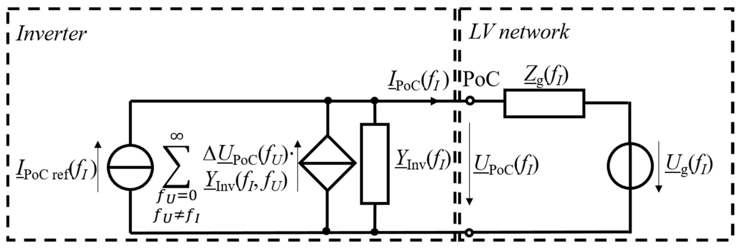
The small-signal characteristics of the entire system model can be separated into the LV network and the inverter, being represented by the coupled Norton model. The inverter is connected to the LV network at the PoC as shown in Figure 1.

2.2. Low-Voltage Network Model

For small-signal studies, the LV network is typically represented by the network impedance Z_g and a voltage source to reflect the background voltage U_g. The background voltage can contain frequencies besides the power frequency f₁, e.g., 50 Hz or 60 Hz, to represent an existing distortion on the network side, e.g., caused by the nonlinear characteristics of other grid-connected devices. This study assumes that the network impedance and the background distortion are independent from the studied inverter. Depending on the specific operating point of the inverter, i.e., the operating power, the disturbances at the PoC can change (U_PoC and I_PoC), but the LV network itself, i.e., the values of Z_g and the spectrum of U_g remain the same.

Public LV networks are generally inductive–resistive in the lower frequency range, e.g., up to the first resonance. This first resonance is often found between 600 Hz and 1.5 kHz [7] and can have significant importance for the harmonic stability of the inverter [8].

2.3. Inverter Model

As the current state of the art, dynamic large-signal time-domain models that are suitable for the harmonic stability analysis are white-box models. The simulation of these models can be very time consuming; therefore, the appropriate solver settings [9] are of major importance for the reliability of the analysis [10] but often challenge the computational power of standard office computers for larger-scale studies. On the other hand, small-signal black-box models can be derived based on measurements or from a known white-box model. Consequently, black-box models can be used for stability analyses without requiring manufacturers to disclose their implementations. Dynamic black-box time-domain modeling, e.g., by the Hammerstein–Wiener model [11,12] and Artificial Neural Networks [13], and its respective analyses [14,15,16] have been studied but were not advanced enough to make reliable statements toward the inverter stability.

2.3.1. Coupled Norton Model

The most advanced small-signal frequency domain black-box model is the coupled Norton model as shown in Figure 1. A current source represents the current I_{PoC ref} measured at a specific reference point. An admittance is used for those currents with the same frequency as the voltage deviation from the measured reference point at the PoC. A voltage-controlled current source reflects currents that result from voltages at different frequencies and are related via a so-called frequency coupling matrix (FCM) Y_Inv that is also called in the literature a harmonically coupled admittance matrix (HAM) [17]. This FCM can be calculated based on the analytical description of the inverter components; thus, simplifications [18] are typically applied due to the mathematical complexity of the analysis.

2.3.2. Measurement-Based Identification

For unknown inverters, the FCM is identified based on measurements, e.g., a frequency sweep is performed as first introduced in [19] and later called the fingerprint with respect to applications on PE devices [20]. For this method, a reference point, i.e., a specific voltage waveform at the PoC, is defined, typically as a sinusoidal waveform with a frequency of 50 Hz and a root mean square (RMS) value of 230 V (nominal voltage). With regard to Figure 1, the applied voltage is represented by the voltage source with the background voltage U_g while the impedance Z_g is set to zero for the model identification.

For the sweep, a single-frequency voltage at integer multiples (harmonics) of the fundamental frequency is superimposed with a specific amplitude and phase angle. For each measurement point, the frequency is increased by one harmonic order. The current response is measured for all currents at the respective frequencies. The elements of the FCM can be calculated with

$${\underset{\_}{Y}}_{\mathrm{I}\mathrm{n}\mathrm{v}}^{}(f_I,f_U)=\frac{{\underset{\_}{I}}_{\mathrm{PoC} i}^{}\left(f_I\right)-{\underset{\_}{I}}_{\mathrm{PoC} \mathrm{ref}}^{}\left(f_I\right)}{{\underset{\_}{U}}_{\mathrm{PoC} i}^{}\left(f_U\right)-{\underset{\_}{U}}_{\mathrm{PoC} \mathrm{ref}}^{}\left(f_U\right)}$$

(1)

For inverters, the amplitude and the phase angle of the voltage at the PoC have an approximately linear impact on the current at the PoC so that the resulting FCM is virtually independent of magnitude and phase angle. While [21] validates the linearity of frequency-dependent voltage and current amplitudes for inverters, ref. [22] indirectly proves the linearity of the respective phase angles. While, originally, ref. [20] introduced a single-frequency sweep based on step changes in frequency, amplitude and phase, ref. [22] proposed to change the phase angle continuously during the measurement to reduce its overall duration by avoiding the step changes that require a wait until the steady state of the next measurement point is reached. An alternative to the single-frequency sweep has been proposed in [21] by applying different sets of multi-frequency distortions to parametrize the FCM based on a small number of measurement points.

2.3.3. Stability Assessment

For the harmonic stability analyses, two main approaches have been applied in the literature. The first approach is based on the Eigenvalue analysis according to the Lyapunov stability [23], e.g., by zero-pole mapping. It qualifies as a detailed analysis by considering the specific design of an inverter including its topology and parameters with respect to the software and hardware components, e.g., to identify the impact of different reference currents for the current control on the inverter stability [5]. The Eigenvalue analysis requires exact knowledge about the poles and zeros that result from the inverter design. For commercial inverters, the design is only known to the manufacturers and usually not disclosed to other parties such as grid operators and research facilities, and consequently, this approach is not applicable.

The second approach is an impedance-based analysis. For simple systems, a stable operation of the entire system can be assumed if the open-loop transfer function does not encircle the point (−1, j0) of the complex plane. The advantage of this approach is the usage of discrete measurement-based values, i.e., the discrete frequency-dependent values of the transfer function instead of an analytical description that would require knowledge of the poles and zeros and consequently the order of the nominator and the order of the denominator, which strictly depend on the manufacturer’s implementation.

As a simplification, the impedance-based criterion for single-phase inverters only considers the linear, time-invariant (LTI) characteristics of the inverter [3], i.e., the main diagonal of the FCM that reflects the admittance. Since the off-diagonal elements of the FCM of single-phase inverters are typically much smaller than the dominating main diagonal elements, the expected contribution to the current response resulting from off-diagonal elements, i.e., frequency couplings, is much smaller than for the main diagonal elements. In practice, any classical instability of the inverter will eventually trigger internal mechanisms, i.e., overvoltage or overcurrent protectors, which will shut it down. Since the dominating currents are related to the main diagonal elements of the FCM, it is assumed to be sufficient to study only the LTI characteristics of single-phase inverters. The LTI characteristics depend on the operating power [24], which is considered quasi-stationary. The changes in the solar irradiance, e.g., due to (partial) shadowing, are much slower than the studied time constants, i.e., changes in the harmonic frequency range. Typically, the inverters start operating at 10% of their rated power up to 100%. Some inverters require a higher minimum power to start their operation.

3. Measurement-Based Stability Assessment

3.1. Inverter Characteristic Identification

3.1.1. Simulated Inverters

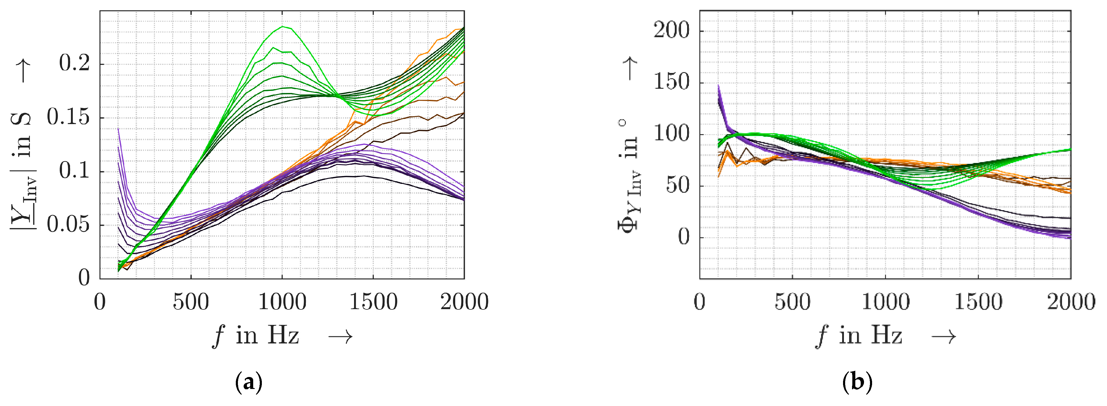
To create different inverter implementations with regard to their design and their impedance characteristics, a modular modeling approach was followed [6]. The admittance characteristics of the four simulation models are depicted in Figure 2.

The suitability of the models has been demonstrated in [25]. The generated implementations are comparable to commercially available inverters and enlarge the database of inverter impedances for large-scale studies. For the frequency sweep, the voltage of the distortion component was set with an amplitude of 10 V and a phase angle of 0°.

3.1.2. Measured Inverters

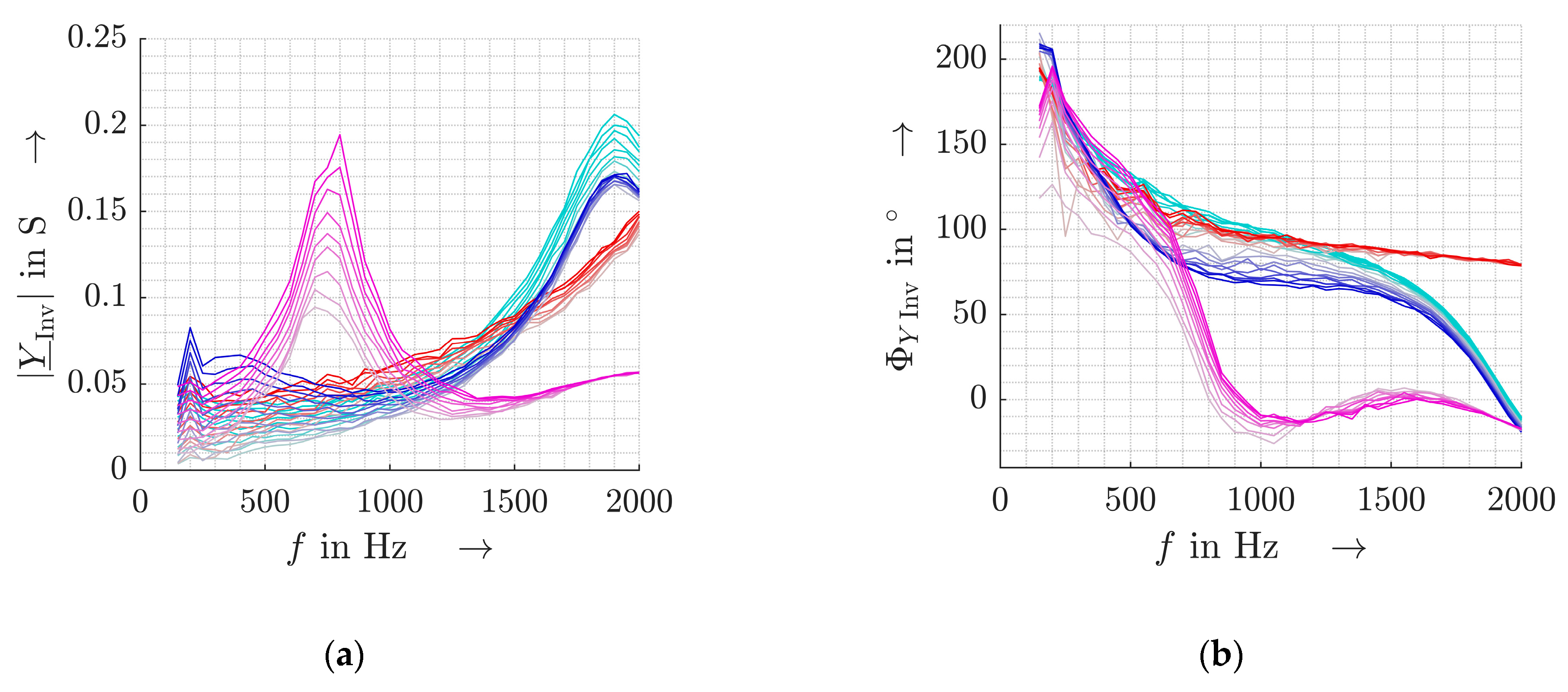
The three commercially available inverters had power ratings of 4.5 kW (inverter I and inverter II) and 3 kW, respectively (inverter III). The admittance characteristics of the three commercial inverters were measured in the laboratory and are presented in Figure 3.

The measurements were recorded with a Dewe-2600 transient recorder, and the respective high-voltage (HV) and LV modules were connected at the PoC in Figure 1. The LV network was represented by a grid simulator (15 kVA) capable of providing a freely programmable voltage harmonic distortion. The voltage was measured directly (HV module). The current was measured using a Rogowski coil connected to the LV module. The measurement uncertainty was determined with a calibrated reference source, the Omicron CMC256-EP. For all laboratory measurements, the acceptable uncertainty was defined as better than 10%, which can be ensured for voltages above 20 mV and currents above 20 mA. The uncertainty for the calculated admittances was consequently better than 20%. The sampling rate of the measurement system was 1 MS/s.

During the measurements in the laboratory, inverter II was shut down for a frequency sweep with an amplitude of 10 V so that, compared to the simulations, an RMS of 5 V and a phase angle of 0° were used for the frequency sweep. In general, it is desirable to set the amplitude of the voltage distortion rather high to reduce the relative impact of the measurement uncertainty on the results.

3.2. Theoretical Stability Analysis

There are different ways to assess the system stability through the Nyquist criterion, e.g., by studying the Nyquist plot. For configurations with simplified LV network representations, i.e., using Z_g and U_g, the open-loop transfer function can be identified with

$${\underset{\_}{I}}_{\mathrm{PoC}}\left(f\right)=\frac{{\underset{\_}{I}}_{\mathrm{PoC}\mathrm{ref}}\left(f\right){\underset{\_}{Z}}_{\mathrm{I}\mathrm{n}\mathrm{v}}\left(f\right)}{{\underset{\_}{Z}}_{\mathrm{I}\mathrm{n}\mathrm{v}}\left(f\right)+{\underset{\_}{Z}}_{\mathrm{g}}\left(f\right)}-\frac{{\underset{\_}{U}}_{\mathrm{g}}\left(f\right)}{{\underset{\_}{Z}}_{\mathrm{I}\mathrm{n}\mathrm{v}}\left(f\right)+{\underset{\_}{Z}}_{\mathrm{g}}\left(f\right)}$$

(2)

in accordance with Figure 1, when only the decoupled part of the inverter model (i.e., ${\underset{\_}{Y}}_{\mathrm{I}\mathrm{n}\mathrm{v}}$ and $I_{\mathrm{P}\mathrm{o}\mathrm{C} \mathrm{r}\mathrm{e}\mathrm{f}}$) representing the LTI characteristics is considered. A reformulation of (2) leads to

$${\underset{\_}{I}}_{\mathrm{P}\mathrm{o}\mathrm{C}}\left(f\right)=\left({\underset{\_}{I}}_{\mathrm{P}\mathrm{o}\mathrm{C}\mathrm{r}\mathrm{e}\mathrm{f}}\left(f\right)-\frac{{\underset{\_}{U}}_{\mathrm{g}}\left(f\right)}{{\underset{\_}{Z}}_{\mathrm{I}\mathrm{n}\mathrm{v}}\left(f\right)}\right)\cdot \frac{1}{1+\frac{{\underset{\_}{Z}}_{\mathrm{g}}\left(f\right)}{{\underset{\_}{Z}}_{\mathrm{I}\mathrm{n}\mathrm{v}}\left(f\right)}}.$$

(3)

When studying the stability, the objective of the analysis is the assessment of the output signal, i.e., ${\underset{\_}{I}}_{\mathrm{P}\mathrm{o}\mathrm{C}}$. Assuming the background voltage to be stable and the inverter impedance to be nonzero, the relevant term of (3) is the ratio of the frequency-dependent network impedance ${\underset{\_}{Z}}_{\mathrm{g}}$ and the frequency-dependent inverter impedance ${\underset{\_}{Z}}_{\mathrm{I}\mathrm{n}\mathrm{v}}$. If Z_Inv and Z_g have a ratio of one (amplitude criterion), the phase difference needs to be below 180°. The phase margin ${\Phi }_{\mathrm{P}\mathrm{M}}$ can be calculated with

$${\Phi }_{\mathrm{P}\mathrm{M}}=180°-{\Phi }_{Z\mathrm{g}}+{\Phi }_{\mathrm{Z}\mathrm{I}\mathrm{n}\mathrm{v}}$$

(4)

and must be positive (phase margin criterion) to indicate the stability of the inverter. Using the above criteria, it is possible to calculate the inductances L_c and the frequencies f_c at which critical conditions will be reached that challenge the stable operation of the inverter. The capacitive phase angles in the low-frequency region of the inverter and the increase in the admittance value with an increasing frequency (cf. Section 3.1) lead to the conclusion that a highly inductive network impedance represents the worst case from the phase angle perspective. Therefore, this study analyzes the harmonic stability for highly inductive network impedances.

3.3. Stability Measurements

In order to validate the approach introduced in Section 3.2, the commercially available inverter I was tested in the laboratory at different operating points, i.e., different operating powers.

3.3.1. Laboratory Setup

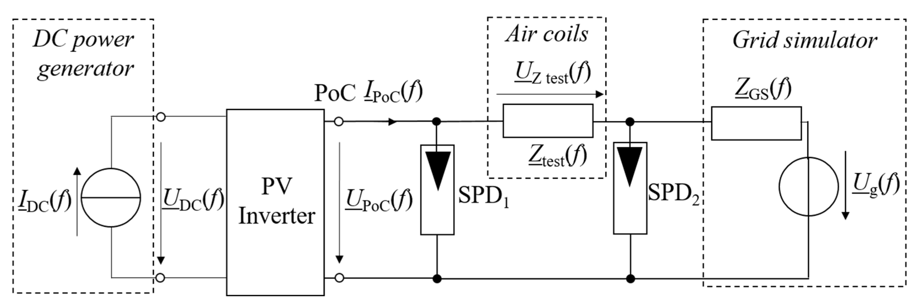
An equivalent scheme of the laboratory setup is presented in Figure 4. The same transient recorder described in Section 3.1.2 and connected to the PoC as in Figure 4 was used for the measurements. The test stand consisted of air coils that formed the test impedance Z_test and enabled the adjustment of the respective inductance L to the values as presented in Figure 5. Furthermore, the grid simulator was non-ideal and had a frequency-dependent impedance Z_GS with an absolute value below 0.3$\Omega$ and a frequency-dependent phase angle of Z_GS that increased from 0 to 90° in the frequency range up to 2 kHz. The impedance of the air coils and the impedance of the grid simulator as well as cables and connectors define the overall test-stand impedance Z_T and can be approximately described with

$${\underset{\_}{Z}}_{\mathrm{T}}\left(f\right)={\underset{\_}{Z}}_{\mathrm{t}\mathrm{e}\mathrm{s}\mathrm{t}}\left(f\right)+{\underset{\_}{Z}}_{\mathrm{G}\mathrm{S}}\left(f\right).$$

(5)

The resistive part Re{Z_T} of the overall test-stand impedance was assumed to be 1$\Omega$. The changes in the inductance of the air coils on the resistive part are negligible and affect only the inductive part and, consequently, Im{Z_T} and the respective phase angle of the test-stand impedance ${\Phi }_{Z\mathrm{T}}$. The inductance of the test impedance Z_test was set by using air coils, which was first introduced as a cost-efficient and flexible test method in [26]. Each block of the air coils consisted of two coils wound into each other, and each air coil had an inductance value between 1 mH and 1.3 mH. By making use of the magnetic coupling through the air gap between two blocks of air coils, the inductance could be adjusted. Along with the possibility of connecting the air coils in parallel and series, a large range of inductance values could be set. In comparison to Figure 1, the LV network impedance Z_g was represented by Z_T at the test stand.

The surge-protection devices (SPD₁ and SPD₂ in Figure 4) for overvoltage protection were rated for 600 V and up to peak impulse currents of 15 kA.

All measurements were performed at room temperature. It should be noted that the range of required inductance values of the air coils depends on the studied inverter and must be determined individually.

3.3.2. Test Scenarios

For the test scenarios, the resulting inductance was increased stepwise. The wiring of the air coils in series and parallel and the length of the air gap between the air coils enabled us to set the overall inductance in large discrete steps (parallel or series connection) and to smoothly adjust it in a very small range (length of air gap). The measured test scenarios with the respective inductance values are listed in

Table 1. Overview of applied inductances during test scenarios.

Test Scenario No.	L Measurement @1 kHz	Test Scenario No.	L Measurement @1 kHz	Test Scenario No.	L Measurement @1 kHz
1	No intended L	5	2380 µH	9	3785 µH
2	1074 µH	6	2385 µH	10	3943 µH
3	1625 µH	7	2600 µH	11	4112 µH
4	1915 µH	8	3500 µH

to test a range of inductance values with regard to the expected critical overall test-stand inductance.

Test scenario 6 was added during the measurements as an additional measurement to study the inverter behavior during test scenario 5 at 4.5 kW in more detail. To compare the operating-point dependency, three operating powers were chosen, i.e., 500 W as the minimum value at which the inverter still operates, 2.5 kW as an operating point that is in the middle of the possible power range and 4.5 kW, i.e., approximately the rated power.

Table 2. Theoretic test-stand scenario analysis.

Test Scenario No.	Impedance Intersection (fcrit)	L Measurement @1 kHz	${\Phi }_{\mathit{Z} \mathit{Inv}}$	${\Phi }_{\mathit{ZT}}$	${\Phi }_{\mathit{PM}}$
4.5 kW
4	619 Hz	1915 µH	−93.1	82.3	4.6°
5	568 Hz	2380 µH	−95.2	83.2	1.6°
6	568 Hz	2385 µH	−95.2	83.2	1.6°
2.5 kW
9	470 Hz	3785 µH	−94.8	84.9	0.3°
10	462 Hz	3943 µH	−95.2	84.8	0°
11	453 Hz	4112 µH	−95.5	85.1	-0.6°
1 kW
10	465 Hz	3943 µH	−93.4	84.8	1.8°
11	455 Hz	4112 µH	−93.8	85.1	1.1°

lists the results of the theoretic analysis for the critical frequency, i.e., the impedance intersection, and the respective phase angles at this frequency when applying the idealized theory with regard to the marginal stability of the test-stand scenarios. In practice, exemplary pre-test measurements indicated minor deviations, i.e., a phase margin of at least 2° instead of the theoretic 0°, to enable a stable operation of the inverter. Therefore, Table 2 lists those theoretically marginally stable scenarios for the respective powers in which the inverter becomes possibly unstable in practice.

3.3.3. Measurement Results

Table 3. Measured results for different operating powers.

Test Scenario No.	Operating Power
	1 kW	2.5 kW	4.5 kW
1	stable	stable	stable
2	stable	stable	stable
3	stable	stable	stable
4	stable	stable	stable
5	stable	stable	stable (multiple attempts to start)
6	not tested	not tested	unstable
7	stable	stable	not started
8	stable	stable	not started
9	stable	stable	not started
10	stable	unstable	not started
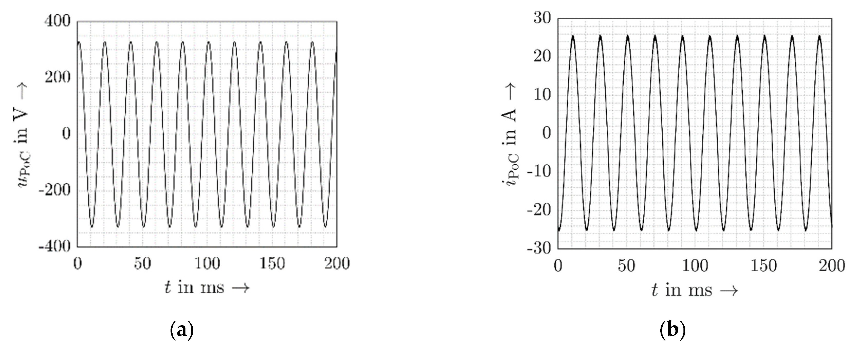
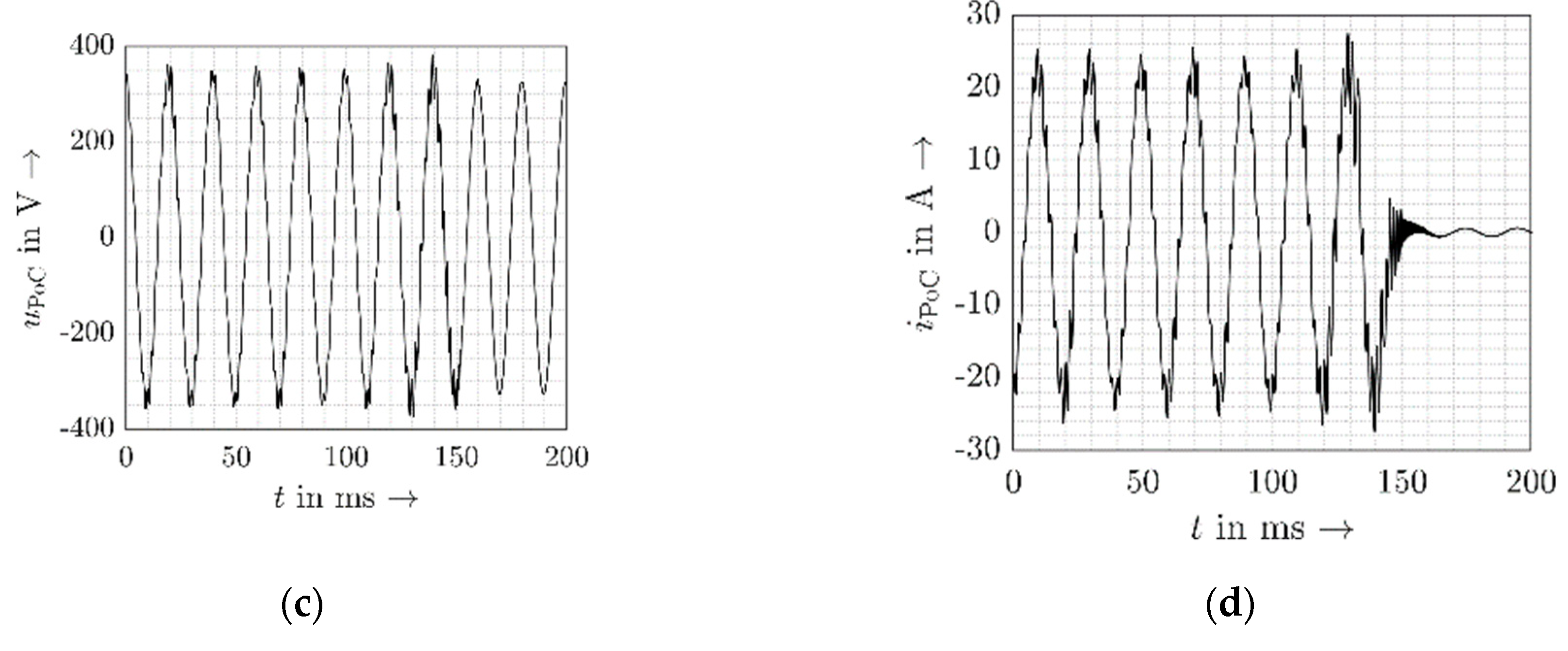
11	unstable	not started	not started

lists the results in terms of the stable and unstable inverter behavior for the three power levels. The abbreviation “n.m.” (not measured) indicates that the listed test scenario was not measured at the respective power. The voltages at the PoC and the respective currents are visualized in Figure 6 exemplarily for measurements at 4.5 kW.

At 4.5 kW in test scenario 5, the inverter required multiple attempts to start and reach a stable operation, i.e., steady state at operating conditions. To characterize this behavior of the inverter further, the inductance was slightly increased in test scenario 6. Therefore, this scenario was only measured at 4.5 kW. The inverter was not able to operate stably and shut down eventually, indicating an insufficient phase margin. For scenarios 7 to 11, at an operating power of 4.5 kW, the inverter did not even start operating due to the high inductance values.

At 2.5 kW, the inverter shut down in test scenario 10 though it was able to reach the operating-point conditions, i.e., injection of reference operating power, for a short time. In test scenario 11, it is not even able to start and shuts down immediately after trying to set the reference conditions. At 1 kW, the inverter is still able to operate stable during test scenario 10 but is not able to operate stable in test scenario 11. In theory, the conditions for which the inverter operates stable or unstable are clearly defined. However, the measurements demonstrate that, in practice, the inverter requires a minimum phase margin to operate reliably stably to handle, e.g., disturbances.

All measurements of instabilities were repeated at least twice, but typically three times to ensure the reproducibility of the measurement.

3.3.4. Measurement Evaluation

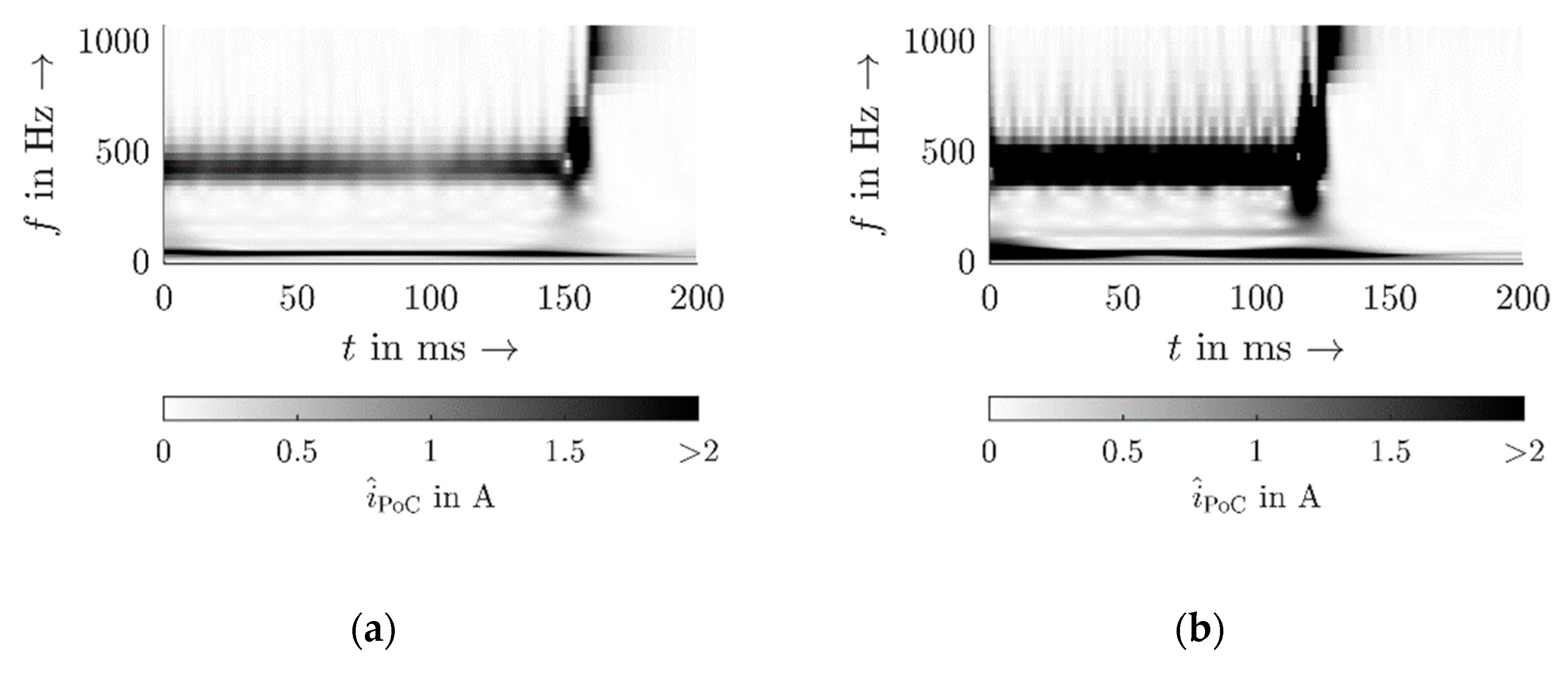
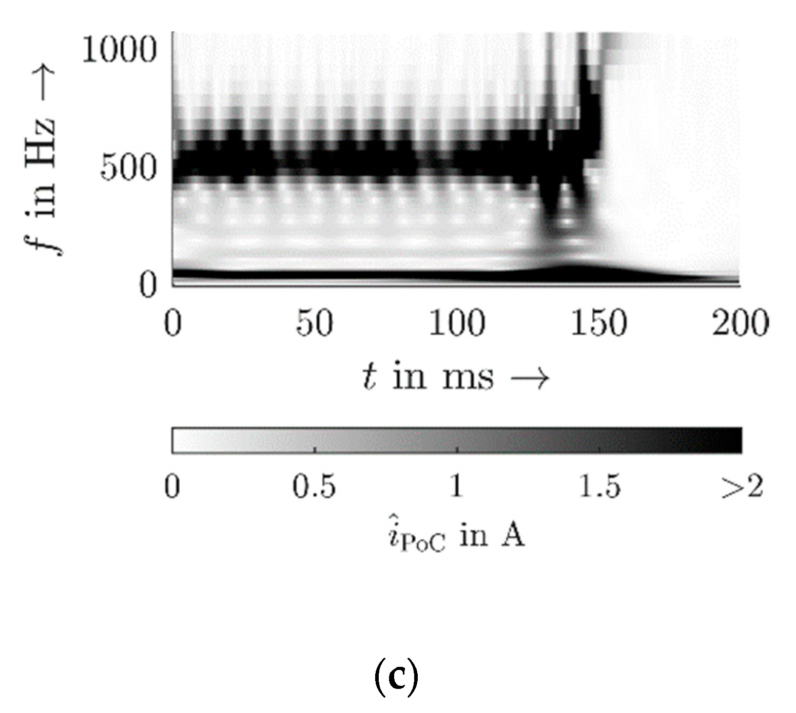
Figure 7 represents the current waveforms of Figure 6 in the wavelet domain, which provides a better visualization, especially in terms of identifying the critical frequency. It shows that, for larger operating powers, the current fluctuation was stronger as well, i.e., the harmonic share was stronger. However, the Heisenberg–Gabor limit [27] prevents the detection of the exact time instance and exact frequency at which the inverter shuts down, since according to

$${\sigma }_t{\sigma }_f\ge \frac{1}{4\pi }$$

(6)

the product of time resolution ${\sigma }_t$ and frequency resolution ${\sigma }_f$ is constant. It is still possible to identify the range of the critical frequency. The dependency of the operating power on the inverter stability becomes obvious when comparing the critical test-stand inductances at 4.5 kW (2.38 mH) and 1 kW (4.11 mH) and validates the theory that the operating point has a significant impact on the inverter stability. Both the measurements and the analysis conclude that the inverter becomes unstable at an inductance of 4.11 mH at 1 kW but only 2.38 mH at 4.5 kW. However, both these values are unrealistically high for public LV networks, which indicates a rather stable behavior of the inverter under realistic grid conditions.

3.3.5. Application on Further Inverters

Section 3.3 proves that the Nyquist criterion holds true for the impedance-based approach if the operating-point dependency is considered and qualifies as a suitable black-box approach. In this section, this approach is applied to all considered inverters to study the operating-power-dependent stability based on the critical inductance L_c that violates both the amplitude and the phase criterion and the respective critical frequency f_c that indicates the critical frequency region. For this analysis, the resistive component of the network impedance is neglected; thus, the studied cases will consider only highly inductive networks.

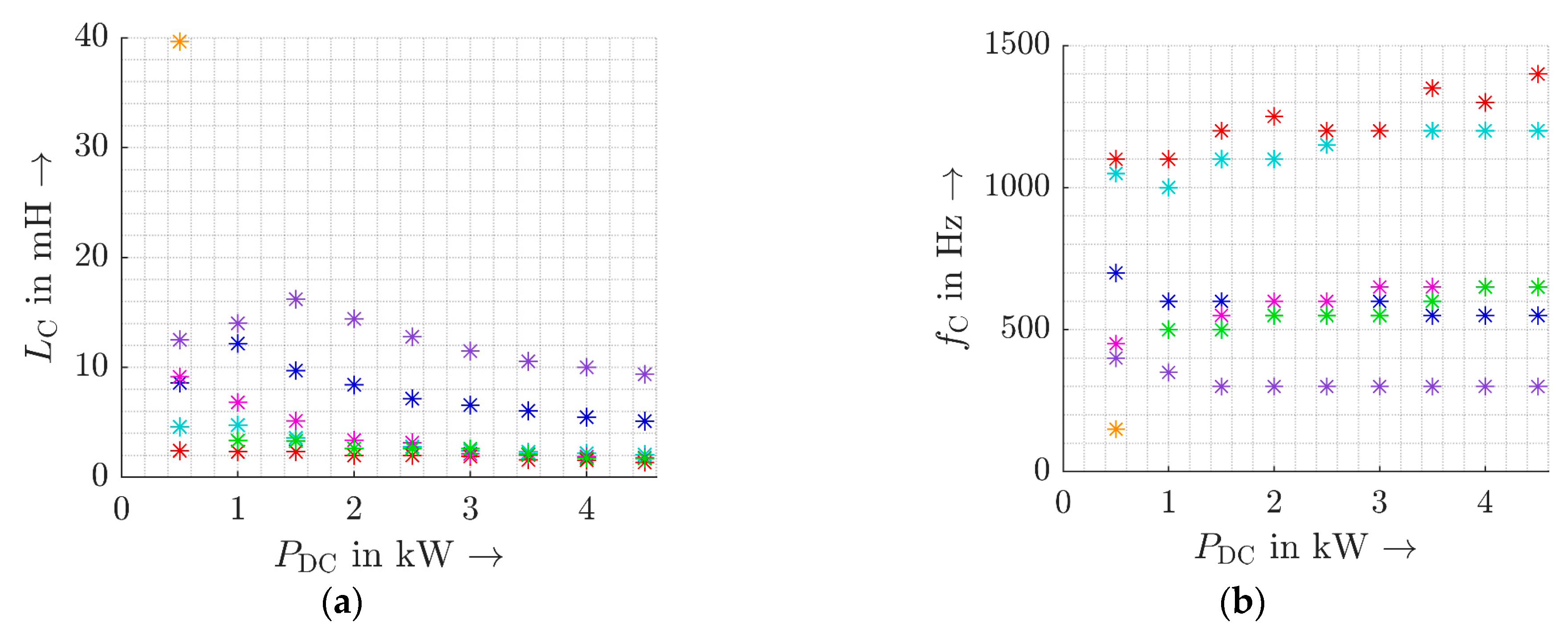
Firstly, it is checked, whether the intersection of the network impedance magnitude and the inverter impedance magnitude for a respective operating power is in the range of the active-frequency region of the inverter. Secondly, the phase margin at the frequency of the impedance intersection is calculated according to (4). Figure 8 shows the calculated critical inductance values for the specific operating power of the inverters as well as the critical frequencies. The change in the critical-frequency region is inverter specific, e.g., inverter B (Figure 8 (red)) changes from 1.1 kHz (500 W) to 1.4 kHz (4.5 kW) by 300 Hz, while inverter I (Figure 8, green) changes from 500 Hz (1 kW) to 650 Hz (4.5 kW) by 150 Hz. Also, the absolute values of the critical frequencies are inverter specific, e.g., inverter II (Figure 8, purple) first becomes critical in the frequency region below 400 Hz and inverter B (Figure 8, red) above 1.1 kHz. Most inverters have a non-monotonous dependency of the critical inductance and the critical frequency related to the operating power. In the case of inverter III (Figure 8, orange), the active-frequency region is only in the very-low-frequency region that is present at an operating power of 500 W. On the other hand, the theoretic critical inductance of another commercially available inverter (red star, Figure 8) was identified as low as 1.35 mH for the worst-case scenario at 4.5 kW. In the field, the network equivalent around resonance can have much higher inductance values due to the resonance amplification than for other frequency regions. The inverter stability is, therefore, prone to low-frequency resonances in the network impedance, which can explain the documentation of a measured instability in [28].

It can be concluded that the individual and operating-point-specific values for the critical inductance and the critical frequency demonstrate the importance of considering not only one but a representative range of operating powers for a generalized small-signal stability analysis [28].

4. Discussion

4.1. Impact of Phase Angle Characteristics of Inverter Impedance

To gain an improved understanding of the operating-point dependency, the phase angle characteristics of the inverter and the related phase criterion can be analyzed in more detail.

With respect to the phase angle characteristics of the inverter impedance, the impact of passive inverter components, e.g., the grid-side filter circuit, and active inverter components, e.g., control and PLL, on the overall impedance characteristics of the inverter is power dependent. For higher powers, the control is typically the dominating impact, while for lower powers, the impact of the grid-side filter circuit is higher on the phase angle characteristics of the inverter impedance. Consequently, the phase angle for higher powers is more in the active region than for low powers. Furthermore, the phase locked loop has a major impact on the overall phase angle characteristics of the inverter. A fast PLL relates typically to a larger bandwidth while a slower PLL relates to a narrow bandwidth. While the narrow bandwidth will reduce the active region of the inverter impedance, a slow PLL increases the response and the reaction time on changes in the voltage at the PoC and can challenge the transient response with regard to the immunity of the inverter due to a large overshoot, e.g., in the current response.

In practice, a common approach to enhance the inverter stability is the introduction of an additional phase angle reserve ${\Phi }_{\mathrm{PR}}$, which accounts for possible phase angle variations in the impedance of the LV network, by adapting (4) to

$${\Phi }_{\mathrm{PM}}=180°-{\Phi }_{Z\mathrm{T}}+{\Phi }_{\mathrm{Z}\mathrm{Inv}}-{\Phi }_{\mathrm{PR}}.$$

(7)

The closer the system operates to the marginally stable case, the lesser the damping. For passive LV networks, this requires a phase angle characteristic of the inverter impedance below 90° (negative resistance), i.e., in the range in which the control is active, and consequently, the inverter injects a current as explained previously.

4.2. Immunity

The small-signal stability is only one aspect of the stable operation of the inverter. For a general statement toward the stable operation of an inverter, the overall immunity of the device must be assessed in more detail in future work. Large-signal perturbations, e.g., changes in the fundamental frequency component of the voltage at the PoC (amplitude or frequency) that can result from load variations, are not considered in the small-signal stability analysis. With respect to small-signal stability analyses, first measurements of the authors indicate that highly distorted voltages at the PoC, even in the absence of a network impedance, can also trigger unwanted shutdowns of the inverters.

Furthermore, a larger resistance, e.g., due to cable connectors, theoretically allows a larger inductance value from the formal stability analysis perspective since the resistance will provide damping to the entire system. However, a larger resistance will also lead to a larger voltage drop, e.g., due to the interaction of the injected current by the inverter itself, other grid-connected devices at the PoC and the network impedance. This component of the voltage drop is even present with an undistorted background voltage. The large resistance can consequently cause high levels of distortion at the PoC and contribute to a shutdown due to the exceedance of the immunity limits of the inverter. Consequently, it is possible that inverter III (Figure 8a, orange) also shuts down, although the required inductance values are unrealistically high compared to the typical impedances of public LV networks. Previous laboratory measurements indicate such a shutdown though a structured measurement method, and the respective evaluation strategy for the holistic stable assessment has not been developed as of yet.

Finally, next to analytic studies and measurements, time-domain simulations can be performed to assess the harmonic stability, but the inverters do not shut down unless the effects that determine the immunity limits, e.g., protection devices that are triggered in commercial devices in case of overvoltages and overcurrents, are properly implemented in simulation models and analytical studies. Protection devices should, consequently, be implemented in future models to represent unstable inverter operations more accurately in simulations.

5. Conclusions

This paper studies the small-signal stability of commercially available single-phase inverters. Due to the lack of details about the individual inverter designs, the presented study is solely based on measurements and, consequently, a black-box approach. The validation of the theory is performed for one commercial inverter using laboratory measurements and applied to six further inverters with either measured or simulated impedance characteristics. It can be concluded that the critical inductance and the critical frequency region that challenge the small-signal stability are unique for each inverter. The results show, furthermore, that the values can differ significantly even for a single inverter depending on the specific operating point, i.e., the operating power of the inverter. Consequently, a reliable small-signal stability analysis must consider a representative range of operating powers. More general, the large diversity of different inverter designs and their individual stability characteristics demonstrate the need for stability assessment strategies and design requirements that are independent of the disclosed topology and parameters, e.g., by individual manufacturers, but generally applicable, especially when the market and the number of installed inverters increase rapidly.

Future work will have to develop a holistic framework to structure all kinds of effects, e.g., the background distortion, that trigger device shutdown and analyze the device immunity. As a second step, a generalized measurement method as well as indices to assess the performance and the grid compatibility of commercially available devices must be developed. Finally, an automatized, measurement-based method for the assessment of the overall stable operation must be designed.

As an extension from inverters to other PE devices, the suitability of the impedance-based criterion for devices with relatively strong frequency couplings, i.e., large off-diagonal elements in the FCM compared to the main diagonal elements, must be studied. Specific indices for the assessment of the suitability need to be introduced. The more dominant the frequency coupling components, the larger will be their impact on the device immunity. Eventually, the frequency coupling components will become relevant for the stable operation of specific types of PE device, e.g., rectifiers.

While the presented study has analyzed the interaction of a single inverter and the public LV network, multi-device black-box interactions must be studied in future work. The increasing penetration of public networks by PE devices affects the network impedance, e.g., its resonances, that, in turn, can affect the stable operation of any grid-connected device.

References

- REN21. Renewables 2022 Global Status Report. 2022. Available online: https://www.ren21.net/gsr-2022/ (accessed on 31 July 2023).
- Wang, X.; Blaabjerg, F. Harmonic stability in power electronic-based power systems: Concept, modeling, and analysis. IEEE Trans. Smart Grid. 2018, 10, 2858–2870. [Google Scholar] [CrossRef]
- Sun, J. Impedance-Based Stability Criterion for Grid-Connected Inverters. IEEE Trans. Power Electron. 2011, 26, 3075–3078. [Google Scholar] [CrossRef]
- Kaufhold, E.; Duque, C.A.; Meyer, J.; Schegner, P. Measurement-Based Black-Box Harmonic Stability Assessment of Single-Phase Power Electronic Devices Based on Air Coils. IEEE Trans. Instrum. Meas. 2022, 71, 1–9. [Google Scholar] [CrossRef]
- Salis, V.; Costabeber, A.; Cox, S.M.; Zanchetta, P. Stability Assessment of Power-Converter-Based AC systems by LTP Theory: Eigenvalue Analysis and Harmonic Impedance Estimation. IEEE J. Emerg. Sel. Top. Power Electron. 2017, 5, 1513–1525. [Google Scholar] [CrossRef]
- Kaufhold, E.; Meyer, J.; Schegner, P. Modular White-Box Model of single-phase Photovoltaic Systems for Harmonic Studies. In Proceedings of the 2019 IEEE Milan PowerTech, Milan, Italy, 23–27 June 2019; pp. 1–6. [Google Scholar]
- Stiegler, R.; Meyer, J.; Höckel, M.; Schori, S.; Scheida, K.; Hanžlík, T.; Drápela, J. Survey of network impedance in the frequency range 2-9 kHZ in public low voltage networks in AT/CH/CZ/GE. In Proceedings of the 25th International Conference on Electricity Distribution, Madrid, Spain, 3–6 June 2019; pp. 3–6. [Google Scholar]
- Kaufhold, E.; Meyer, J.; Schegner, P. Impact of grid impedance and their resonance on the stability of single-phase PV-inverters in low voltage grids. In Proceedings of the 2020 IEEE 29th International Symposium on Industrial Electronics (ISIE), Delft, The Netherlands, 17–19 June 2020; pp. 880–885. [Google Scholar]
- Hadjidemetriou, L.; Kyriakides, E. Accurate and efficient modelling of grid tied inverters for investigating their interaction with the power grid. In Proceedings of the 2017 IEEE Manchester PowerTech, Manchester, UK, 18–22 June 2017; pp. 1–6. [Google Scholar]
- Kaufhold, E.; Meyer, J.; Schegner, P.; Abdelsamad, A.S.; Myrzik, J.M.A. Comparison of solvers for time-domain simulations of single-phase photovoltaic systems. In Proceedings of the 2020 International Conference on Smart Grids and Energy Systems (SGES), Perth, Australia, 23–26 November 2020; pp. 550–555. [Google Scholar]
- Patcharaprakiti, N.; Kirtikara, K.; Monyakul, V.; Chenvidhya, D.; Thongpron, J.; Sangswang, A.; Muenpinij, B. Modeling of single phase inverter of photovoltaic system using Hammerstein–Wiener nonlinear system identification. Curr. Appl. Phys. 2010, 10, S532–S536. [Google Scholar] [CrossRef]
- Abdelsamad, A.S.; Myrzik, J.M.A.; Kaufhold, E.; Meyer, J.; Schegner, P. Voltage-Source Converter Harmonic Characteristic Modeling Using Hammerstein-Wiener ApproachModélisation des caractéristiques harmoniques d’un convertisseur tension-source à l’aide de l’approche Hammerstein-Wiener. IEEE Can. J. Electr. Comput. Eng. 2021, 44, 402–410. [Google Scholar] [CrossRef]
- Kaufhold, E.; Grandl, S.; Meyer, J.; Schegner, P. Feasibility of Black-Box Time Domain Modeling of Single-Phase Photovoltaic Inverters Using Artificial Neural Networks. Energies 2021, 14, 2118. [Google Scholar] [CrossRef]
- Wiesermann, L.M. Developing a Transient Photovoltaic Inverter Model in Opendss Using the Hammerstein-Wiener Mathematical Structure. Ph.D. Dissertation, University of Pittsburgh, Pittsburgh, PA, USA, 2017. [Google Scholar]
- Kaufhold, E.; Meyer, J.; Schegner, P. Measurement Framework for Analysis of Dynamic Behavior of Single-Phase Power Electronic Devices. Renew. Energy Power Qual. J. 2020, 18, 494–499. [Google Scholar] [CrossRef]
- Kaufhold, E.; Meyer, J.; Schegner, P. Transient response of single-phase photovoltaic inverters to step changes in supply voltage distortion. In Proceedings of the 2020 19th International Conference on Harmonics and Quality of Power (ICHQP), Dubai, United Arab Emirates, 6–7 July 2020; pp. 1–6. [Google Scholar]
- Sun, Y.; Zhang, G.; Xu, W.; Mayordomo, J.G. A Harmonically Coupled Admittance Matrix Model for AC/DC Converters. IEEE Trans. Power Syst. 2007, 22, 1574–1582. [Google Scholar] [CrossRef]
- Rygg, A.; Molinas, M.; Zhang, C.; Cai, X. Coupled and decoupled impedance models compared in power electronics systems. arXiv 2016, arXiv:1610.04988. [Google Scholar]
- Hall, S.R.; Wereley, N.M. Generalized Nyquist Stability Criterion for Linear Time Periodic Systems. In Proceedings of the 1990 American Control Conference, San Diego, CA, USA, 23–25 May 1990; pp. 1518–1525. [Google Scholar]
- Cobben, S.; Kling, W.; Myrzik, J. The Making and Purpose of Harmonic Fingerprints. In Proceedings of the 19th International Conference on Electricity Distribution, Vienna, Austria, 21–24 May 2007; pp. 21–24. [Google Scholar]
- Kaufhold, E.; Meyer, J.; Schegner, P. Fast measurement-based identification of small signal behaviour of commercial single-phase inverters. In Proceedings of the 2021 IEEE 11th International Workshop on Applied Measurements for Power Systems (AMPS), Cagliari, Italy, 29 September–1 October 2021; pp. 1–6. [Google Scholar]
- Gallo, D.; Langella, R.; Luiso, M.; Testa, A.; Watson, N.R. A New Test Procedure to Measure Power Electronic Devices’ Frequency Coupling Admittance. IEEE Trans. Instrum. Meas. 2018, 67, 2401–2409. [Google Scholar] [CrossRef]
- Lyapunov, A.M. The general problem of the stability of motion. Int. J. Control. 1992, 55, 531–534. [Google Scholar] [CrossRef]
- Kaufhold, E.; Müller, S.; Meyer, J.; Myrzik, J.; Schegner, P. Impact of DC power on the small signal characteristics of single-phase phtovoltaic inverters in frequency domain. In Proceedings of the 2023 8th Internaitonal Conference on Clean Electrical Power (ICCEP), Terrasini, Italy, 27–29 June 2023; pp. 1–6. [Google Scholar]
- Kaufhold, E.; Meyer, J.; Schegner, P. A modular time-domain model of single-phase photovoltaic inverters enabling realistic harmonic large-scale simulations in low voltage networks. In Proceedings of the 2022 IEEE 20th International Power Electronics and Motion Control Conference (PEMC), Brasov, Romania, 25–28 September 2022; pp. 481–486. [Google Scholar]
- Kaufhold, E.; Meyer, J.; Schegner, P. Measurement-Based Black-Box Harmonic Stability Analysis of Commercial Single-Phase Inverters in Public Low-Voltage Networks. Solar 2022, 2, 64–80. [Google Scholar] [CrossRef]
- Gabor, D. Theory of communication. Part 1: The analysis of information. J. Inst. Electr. Eng. Part III Radio Commun. Eng. 1946, 93, 429–441. [Google Scholar] [CrossRef]
- Höckel, M.; Gut, A.; Arnal, M.; Schild, R.; Steinmann, P.; Schori, S. Measurement of voltage instabilities caused by inverters in weak grids. CIRED Open Access Proc. J. 2017, 2017, 770–774. [Google Scholar] [CrossRef]