1. Introduction
Developing a country’s economy relies heavily on having access to sufficient energy resources [
1,
2]. In this sense, the energy demand has surged in recent decades due to population growth, rapid urbanization, and social needs [
3]. According to a study by [
2], the use of fossil fuels by energy companies to produce complementary energy contributes significantly to pollution. Therefore, it is crucial to halt this practice to minimize its negative consequences. As a solution, energy companies have taken measures by adopting alternative energy sources to not only lessen their environmental impact but also meet the growing energy demands [
4].
One of the most significant sources is solar energy, which has received much attention in the last decade among all the other renewable energy systems [
5,
6]. The utilization of solar energy as a source of electricity has been a prevalent practice for years, with photovoltaic (PV) panels being the primary tool for this purpose. However, it is notable that the power generated by a PV panel is not solely determined by its design and construction. Several external factors, mainly the PV panels’ environmental variables, perform a crucial role in defining the panel’s power output. Additionally, intrinsic factors that are typical of semiconductors also limit the amount of power generated. Therefore, having a comprehensive grasp of the various environmental factors and the limitations of semiconductors is crucial for making the most efficient use of solar energy [
7].
Multiple studies have shown that the efficiency of PV cells can be affected by interruptions and disruptions caused by fluctuating weather conditions [
8,
9,
10,
11,
12]. The studies emphasize the importance of implementing reliable models in PV systems for energy production planning, maintenance, failure detection, and adjustments in large systems by decision making using the collected data.
The use of artificial intelligence (AI) has increased considerably in recent years due to its ability to model and solve complicated computational tasks [
13], improve the measurement equipment’s profitability [
14,
15], predictive analytic tools [
16], pattern recognition and classification [
17], and coefficient estimator in heat transfer applications [
18], and model a complex relationship without expert knowledge [
19].
Considerable advances have been made in modeling and forecasting the energy output of solar panel systems. While regressor models can estimate current values based on specific inputs, they only provide predicted actual values. Forecasting, on the other hand, can predict future values based on past and current inputs. The length of the forecast can vary depending on the method used, ranging from short-term (a few seconds to a few minutes) to long-term (a few months to a year or more) methods [
1,
20].
In this context, several artificial intelligence (AI) and machine learning (ML) techniques have been employed to model energy generated by a photovoltaic (PV) system. These techniques enclose a variety of methodologies, including artificial neural networks (ANNs), k-nearest neighbors (KNNs), extreme learning machines (ELMs), and support vector machines (SVMs) [
21,
22,
23]. These diverse approaches reflect the multidimensional nature of energy estimation in PV systems, each offering unique strengths and applicability depending on specific project requirements and objectives.
Artificial neural networks (ANNs) are highly effective for modeling energy estimations in photovoltaic (PV) panels due to several reasons. ANNs have the ability to perform nonlinear modeling [
21], learn from available data without relying on explicit mathematical equations [
22,
23], extract features to determine the most influential factors in energy estimation [
17], and can be scaled to handle large and complex datasets. Additionally, ANNs have the potential for high generalization on unseen data when properly trained and can continuously learn and integrate with IoT sensors to provide real-time monitoring and adaptive energy estimations [
21,
22,
23].
While ANNs offer numerous advantages, it is important to note that their effectiveness depends on factors such as data quality, model architecture, and training methods. Researchers often choose ANNs for PV energy estimation due to their capacity to handle complex, dynamic, and nonlinear relationships inherent in photovoltaic systems, but the choice should always be guided by the specific goals and characteristics of the project.
Different models based on artificial neural networks (ANNs) have been developed to estimate or forecast the output energy of photovoltaic (PV) systems, each utilizing different sets of input data. Sangrody et al. (2017) employed ANNs to estimate PV output energy using weather data based on sky cover, humidity, and temperature [
24]. Verma et al. (2016) utilized ANNs with input variables, including temperature, cloud cover, wind speed, humidity, rainfall, and panel elevation–azimuthal angle [
25]. In this research, the authors develop linear regressor, logarithmic, and polynomial models to compare them against the ANN instance. The authors conclude that the ANN model gives the minimum error and is the most reliable technique. Similar works develop forecasting models using mainly solar radiation with variations in weather data [
22,
26,
27].
These models demonstrate how ANNs can effectively adapt to different input data sources, highlighting their ability to capture the complex relationship between environmental variables that affect PV energy generation. However, it is worth noting that the models mentioned in this study mostly rely on meteorological data available online or a mix of local measurements with online data.
It is important to keep in mind that online or meteorological data come from a different location than the actual location of the PV system. In addition, some cited papers need more fundamental information, like sampling frequencies and the amount of data used for modeling. This missing information could result in insufficient continuity to track weather intermittency that affects the PV cells.
When utilizing online or meteorological data for a PV system, it is critical to keep in mind that the data originate from a separate location from the actual system. It is also significant that certain referenced papers should necessitate supplementary essential information, such as sampling frequencies and the quantity of data employed for the training process. In the absence of such details, deficient continuity in monitoring weather intermittency may occur, potentially impacting the model’s performance.
It was found that only a limited number of models are based on real-time and on-site measurements for PV applications [
11,
28,
29]. Notably, these authors highlighted the significance of installing IoT systems close to PV systems to gather real-time data, especially in countries where micro-climates can differ drastically between PV and meteorological locations.
The present paper proposes a case study conducted in Michoacan, Mexico, where an Internet of Things (IoT) device is employed for real-time logging of on-site data related to electrical and weather aspects of a photovoltaic system. The designed IoT device gathers data about radiation levels, temperature, humidity, and electrical power parameters, specifically the panel’s voltage and current, with a consistent sampling frequency of 5 min. The data gathering is spanned over multiple months, allowing for the assembly of a more suitable dataset, which subsequently serves as the foundation for the modeling phase of the study.
This first approach uses a set of 1000 instances to train and compare different ANN topologies. As a result, a satisfactory topology has a root mean squared error (RMSE) of 0.255326464 for power-delivering estimations. Next, a non-autoregressive neural network (Non-AR-NN) model is developed to forecast the future power value. The model adopted has an RMSE of 0.1160.
Thus, the present paper is organized in the following way.
Section 2 gives a general description of modeling using ANNs and the procedure followed in this research until the selection of the best model settings.
Section 3 discusses the model’s performance in predicting power estimations using environmental variables. Also, the Non-AR-NN model is discussed to predict future estimations. Finally,
Section 4 gives the final arguments about the finds in this paper.
2. Materials and Methods
The present section describes the basics of artificial neural networks (ANNs) and the general procedure for developing models based on ANN regressors. Then, details about the designed devices are given for collecting data. Next, preprocessing and correlation analysis are described to define the ANN model and its training process.
2.1. Artificial Neural Networks Basics
Artificial neural networks (ANNs) are computational models inspired by the structure and functioning of biological neural networks in the human brain [
30]. The ANN consists of interconnected artificial neurons, also called processing units, organized in layers: an input layer, one or more hidden layers, and an output layer [
31].
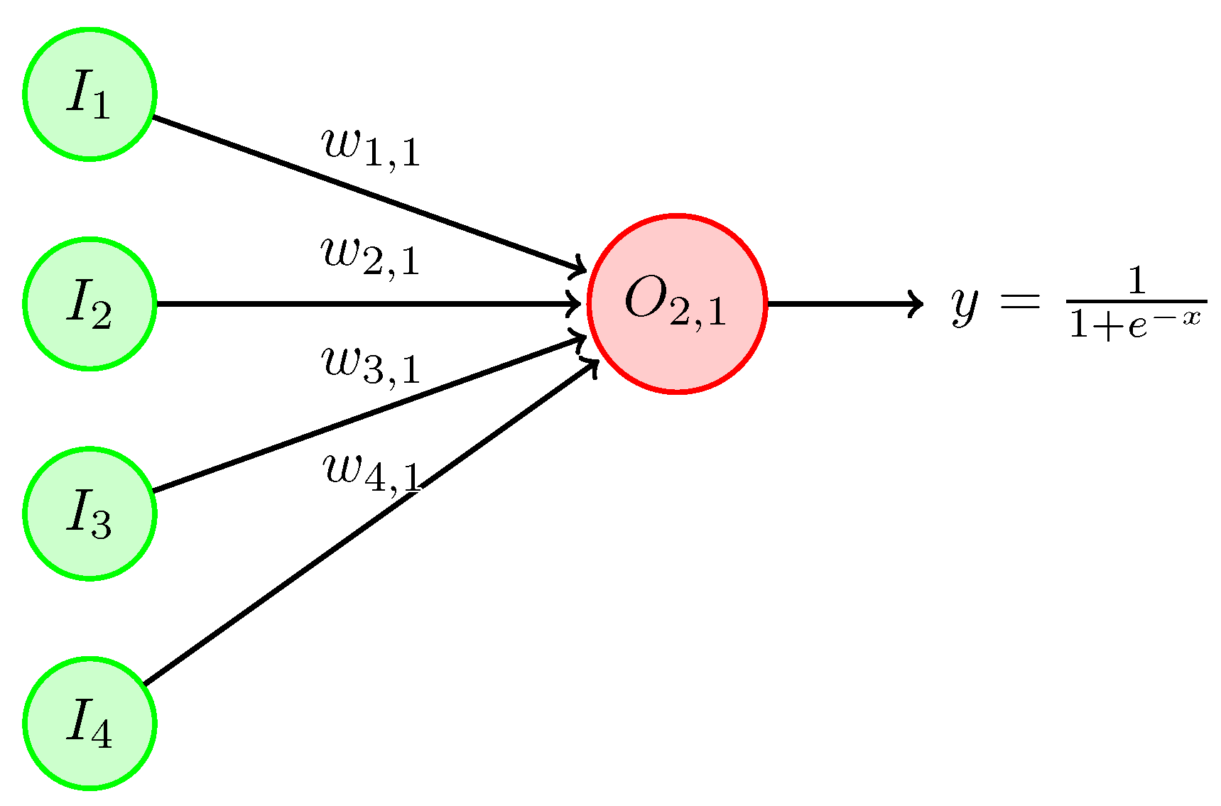
The perceptron is the fundamental processing unit; see
Figure 1. It is a simple mathematical model that takes multiple input values (
), each multiplied by a corresponding weight (
), and then sums up these weighted inputs (
X). The resulting sum is passed by an activation function to produce the output (
). Different versions of this topology incorporate a bias input (
b) in addition to the features.
Thus, the perceptron operation can be described mathematically as follows:
where
is the sigmoid activation function. However, this function can also be the hyperbolic tangent function, linear, RELU, among others.
The activation function introduces non-linearity, allowing perceptron and subsequent ANNs to model complex patterns and relationships in data. It is well known that a single perceptron can perform simpler linear classification problems [
31,
32]. On the other hand, multiple interconnected perceptron architectures, organized in layers, can handle more complex tasks.
The versatility of artificial neural networks (ANNs) is remarkable, as they can employ both linear and non-linear activation functions and different combinations of both. That is why they have proven to be useful in a wide range of scopes, including control, pattern recognition, classification, forecasting, and non-linear regressors [
33].
The focus of this study is on universal function approximation or non-linear regression modeling. Thus, analytical models, which rely on the physical relationships within the modeled system, are a popular method for developing models in this context. These models are known as “White-box” and require extensive system knowledge. Alternatively, there is a second option known as “Black-box” models, which use statistical and machine learning methods to directly predict the system’s output. It is also important to consider a hybrid model, known as the “Grey-box”, which combines both techniques for more accurate results. However, most studies in non-linear applications tend to rely heavily on the “Black-box” model approach [
28].
2.2. Implementation of an ANN Regressor
The typical process of creating a regressor or classifier ANN involves these steps: data preparation, network architecture selection, loss function definition, optimizer choice, training the ANN, hyper-parameter tuning, model evaluation, and prediction. In general terms, each step can be defined as follows:
The process of data preparation involves collecting and preprocessing data from experiments or polls. A typical preprocessing step is scaling and normalizing input features and target values. These input features and targets are commonly known as instances; then, instances are commonly randomly grouped as training and testing datasets.
The network architecture stage considers the architecture by determining the number of layers and neurons per layer, as well as the activation functions. For regression applications, the final layer should have a single neuron with a linear activation function.
The choice of the loss (cost) function is crucial in creating accurate models. Metrics such as mean squared error (MSE) or mean absolute error (MAE) can lead to different outcomes.
During the training stage, the neural network’s weights and bias can be updated using various numeral optimizers such as gradient descent, stochastic gradient descent, batch gradient descent, mini-batch gradient descent, and adaptive moment estimation (Adam).
The model will be updated using the prepared dataset and the previously defined neural network architecture. The training process will be monitored by observing the loss decrease by the optimizer. Then, the model’s performance is evaluated over a validation dataset.
Evaluating the model’s performance requires testing with various hyper-parameters, such as learning rate (), batch size (n), and number of epochs.
After completing the training stage, the model’s performance is evaluated on a different test dataset. Metrics such as mean squared error, mean absolute error, and R-squared are used to determine the model’s prediction accuracy. Nevertheless, it is highly recommended to use the same previously defined loss function.
Finally, if the initial results are not satisfactory, it is possible to try adjusting the network architecture, hyper-parameters, collecting more data, or even including additional inputs to improve the model’s performance.
2.3. Non-Autoregressive Neural Networks
Considering the previous description about the ANN and its implementations as a regressor model, the non-autoregressive neural network (Non-AR-NN) variant with sequential data input topology can be introduced. The Non-AR-NN is a type of ANN specifically designed for processing data sequences, also known as time series. Unlike traditional feed-forward neural networks, Non-AR-NNs can have a sequence of data as input, such as a time series of values or a sequence of tokens in natural language. Each element in the sequence is treated as an input feature at a specific time step emulating kind of sliding window lag. This non-recurrent structure allows for parallel prediction and faster computing without sequential constraints, making it capable of modeling temporal dependencies.
2.4. Data Preparation: IoT Device and Experimental Setup
Developing accurate models requires the collection and validation of representative data. To accomplish this, we have designed an IoT measurement prototype that gathers voltage and current measurements and environmental factors like radiation levels, temperature, and humidity on-site for the modeling PV system.
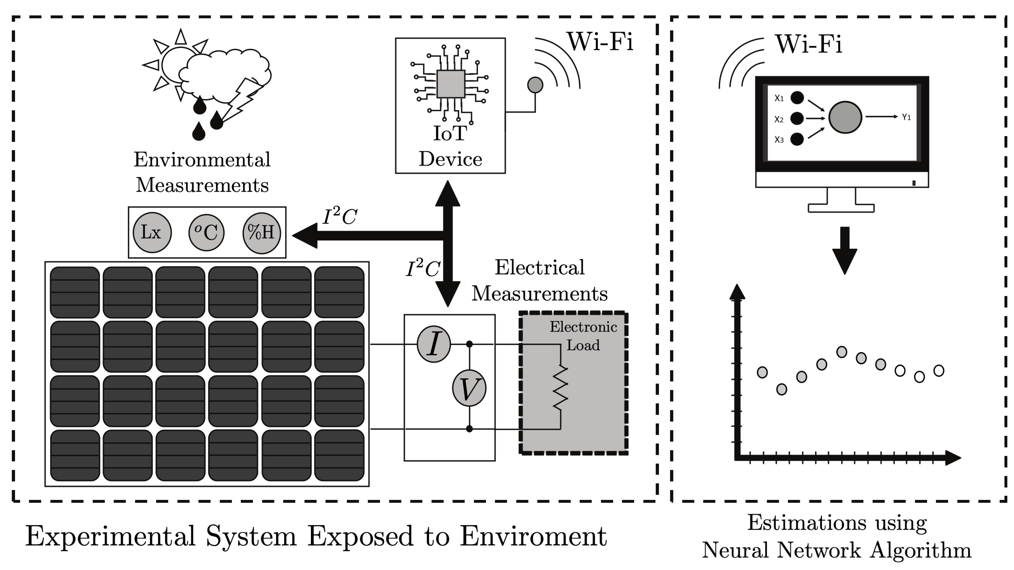
Figure 2 shows the general methodology for gathering and downloading data through the IoT device using a PC.
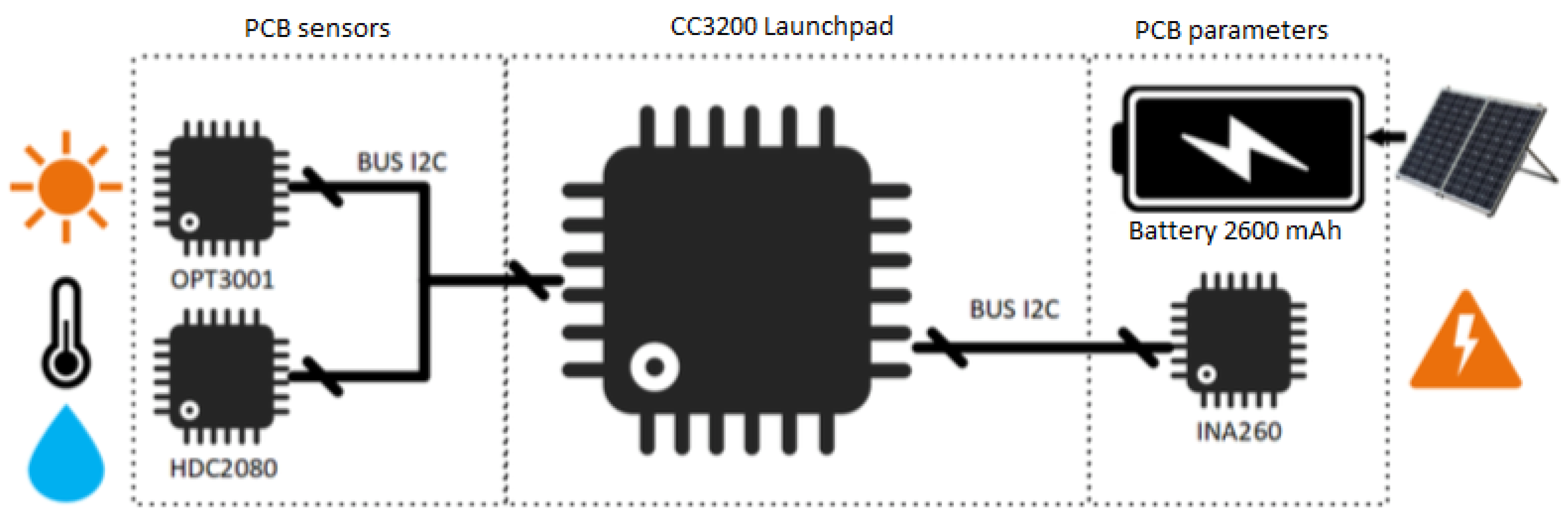
The designed IoT device is a small circuit based on the CC3200 microcontroller and embeds three sensors, an instrumentation amplifier, and a rechargeable battery as the power supply; see
Figure 3. The sensors communicate via
, a protocol that enables digital handshaking between microcontrollers and sensors. The microcontroller features a web server that facilitates storing and managing logged data for further processing. Then, the complete system uses the battery to enable all the circuitry and features of the IoT device supported by a small solar panel that charges it, making it efficient and self-powered.
The symbols on the left in
Figure 3 are the weather sensors and the
OPT3001 and
HDC2080 integrated circuits. The
OPT3001 is a light sensor with a
resolution, including an upper limit of 128
. However, an attenuating glass has been used to extend 55% of the device limit; a calibration procedure was conducted using the commercial digital luxometer
MASTECH ms6612. Next, the
HDC2080 sensor measures relative humidity (RH) and temperature. For temperature, the sensor has a ± 0.2 °C resolution with ranges of −40 °C to 85 °C, while the RH sensor gives measurements with a
resolution.
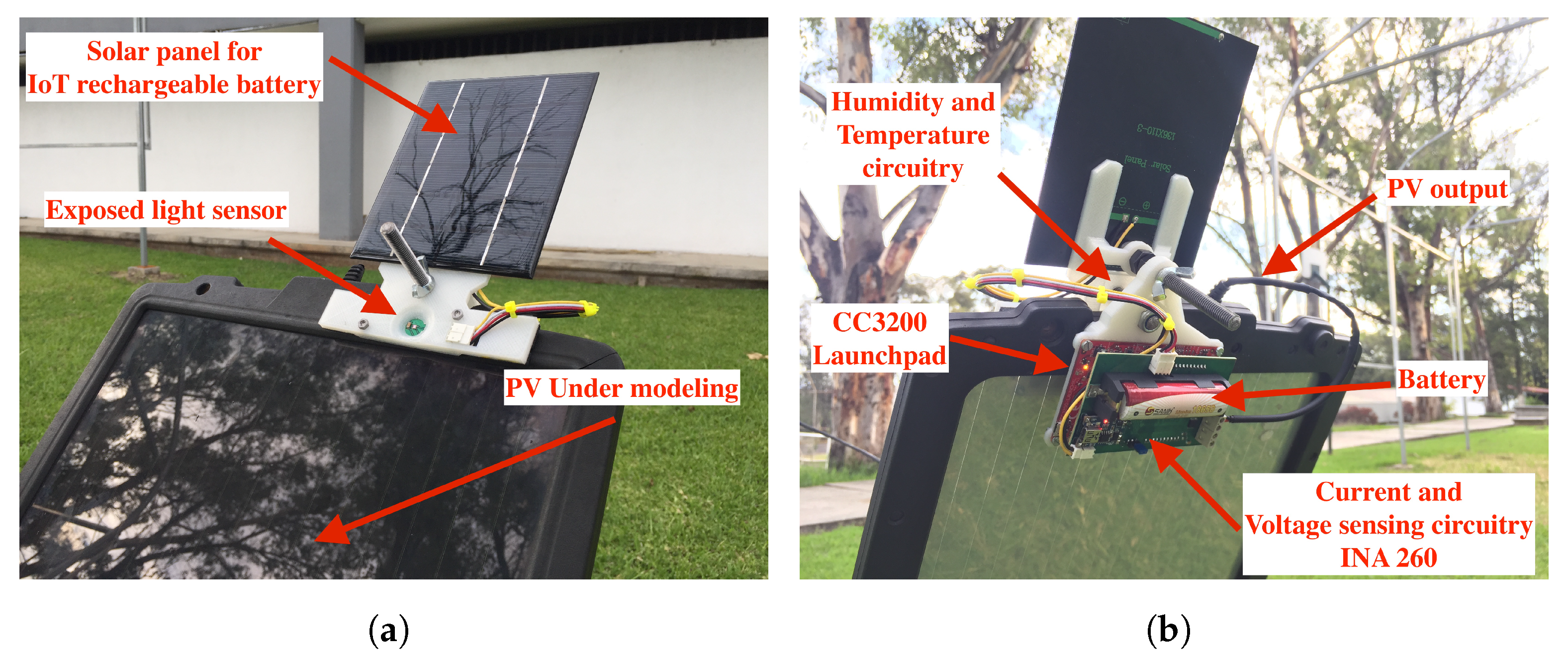
Figure 4, shows a comprehensive view of the primary PV and IoT systems from both the front and rear. The front view highlights the lighting sensor fixture alongside humidity and temperature sensors. The rear view (
Figure 4b) depicts the IoT circuitry implemented for measuring the PV’s current and voltage mounted over the CC33200 launchpad.
Before implementing the ANN model, the collected data are compared with readings from a commercial meteorological station that is installed in a close location as the IoT system. The data from both sources include information on solar radiation, humidity, and temperature. To ensure a correct comparison, data are normalized using Equation (
2), since the measurements were obtained from different equipment:
where
is the actual value to be normalized,
is the minimum value of the entire data set, and
is the maximum value of the entire data-set. The normalization process is utilized in subsequent stages, such as correlation analysis and training.
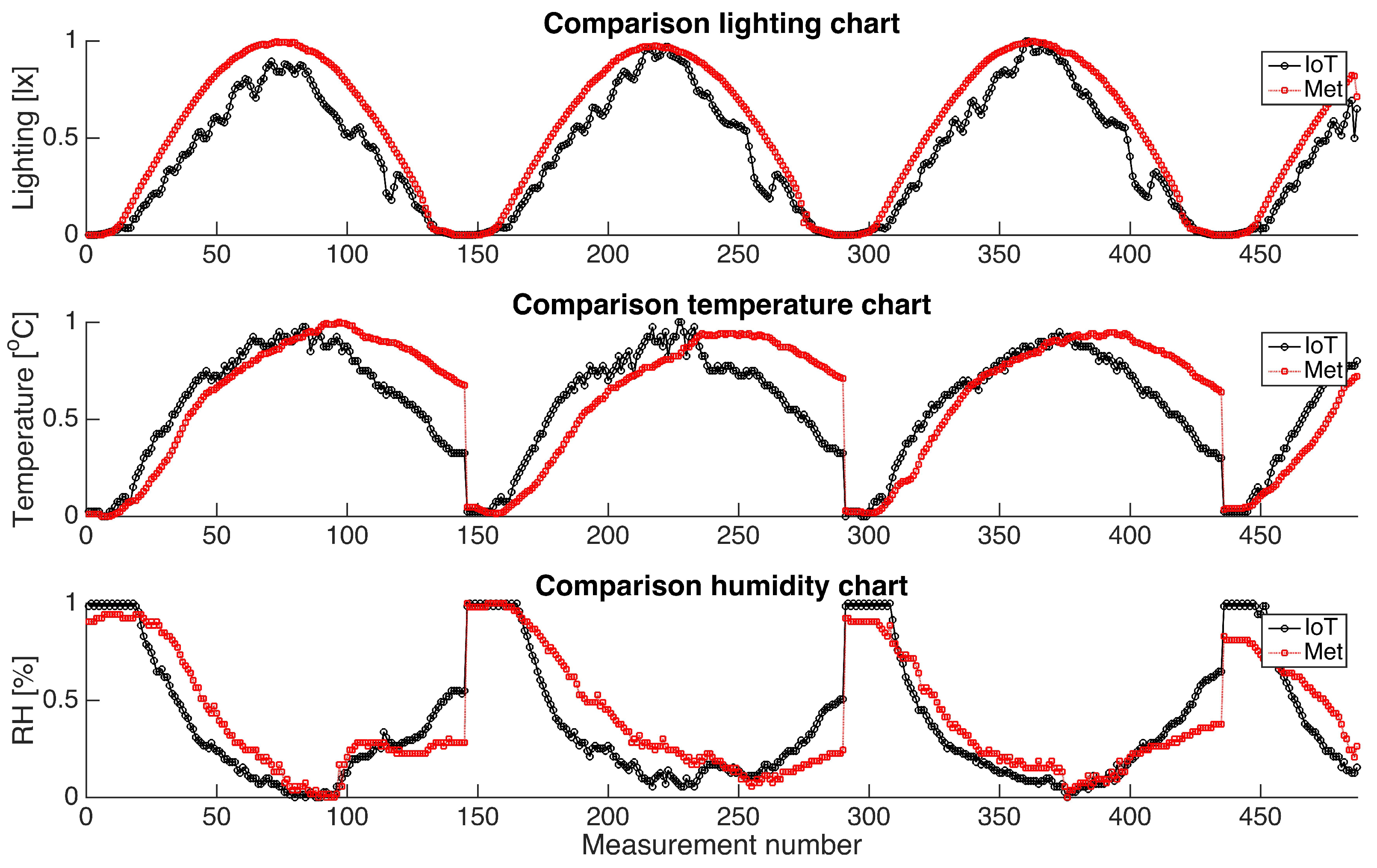
Figure 5 in this paper illustrates a comparison between the measurements gathered by the IoT system and those recorded by the meteorological station. The observed slight variations between the datasets can be attributed to the following installation factors: the lightning sensor angles, the temperature sensors’ location, and methods for humidity measurements.
After comparing the RMSE values, it was found that the error rates for lighting, temperature, and humidity are 0.096, 0.1796, and 0.1491, respectively. The temperature measurement error is primarily caused by the sensor location. The IoT system collects data on the panel’s temperature, which is crucial in identifying its impact on the panels’ efficiency. However, the meteorological station measures ambient temperature, leading to significant differences in the data.
Table 1 presents a selection of measurements acquired by the IoT system. Within the table, the initial column designates the timestamp for each measurement. Subsequently, the second column describes lighting data expressed in lux, followed by temperature in the third column, humidity in the fourth column, current in the fifth column, voltage in the sixth column, and, finally, the computed power values are listed in the seventh column.
Within the context of data preparation for training the artificial neural network (ANN), an essential step involved the selection and preprocessing of data.
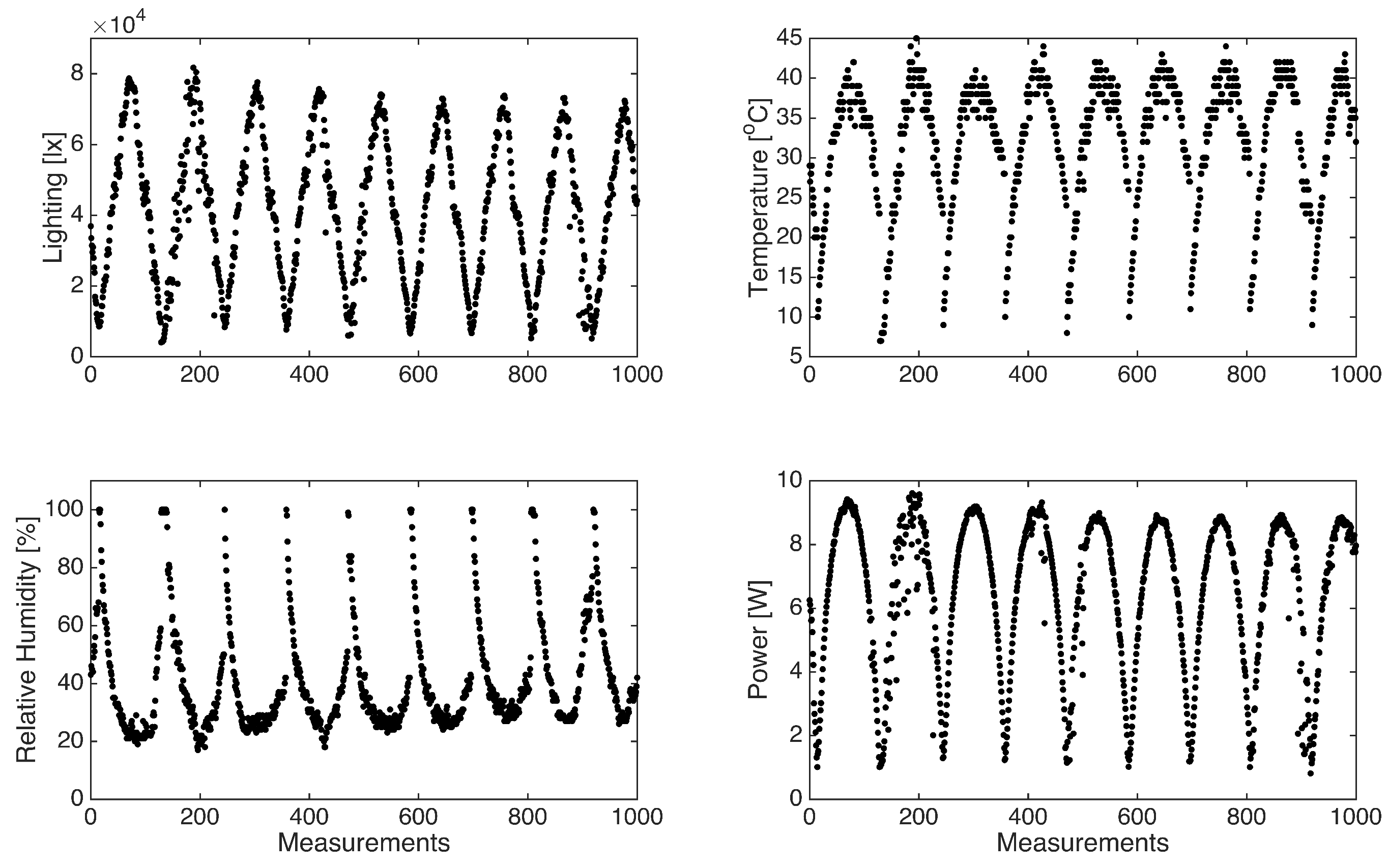
Figure 6 provides an illustrative representation of measurements during nine consecutive days, containing all variables acquired by the IoT system. A particular data filtering process is implemented to enhance the dataset’s relevance and suitability for solar power estimation to exclude measurements recorded during night-time periods, as these measurements are non-contributory to the photovoltaic system’s power generation dynamics. This preprocessing step ensures that the dataset used for training the ANN encloses only the pertinent observations, thereby optimizing the model’s capacity for accurate power output predictions.
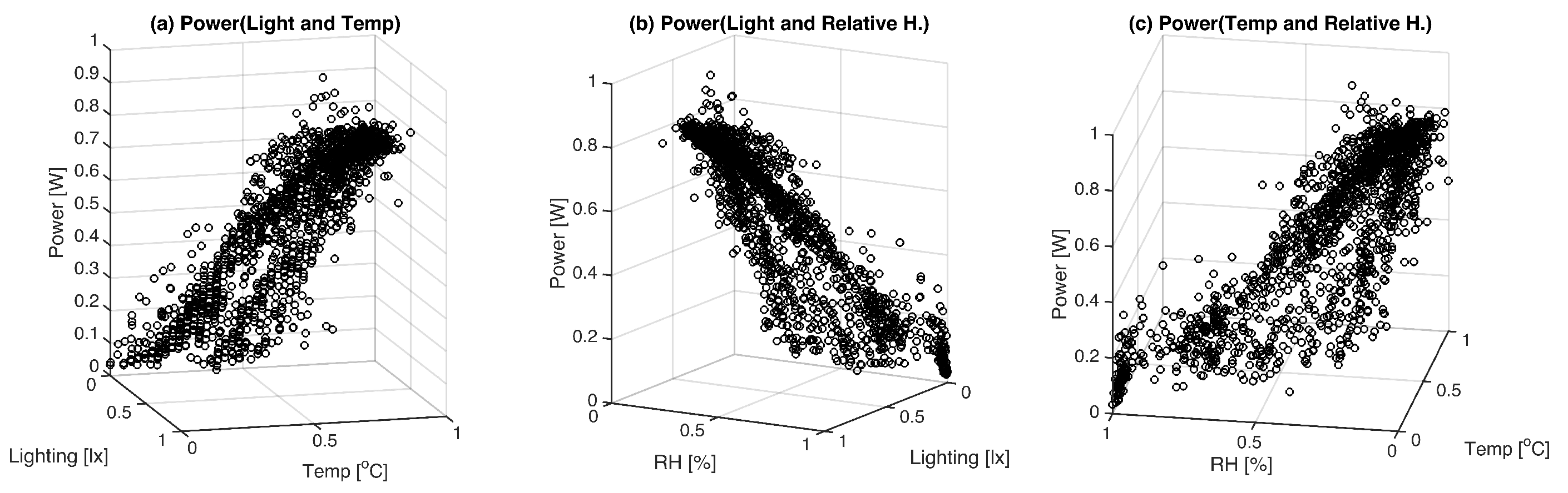
Next,
Figure 7 presents three correlation plots, each proposing distinct relationships: (a) examining the interaction between luxes, temperature, and power; (b) observing the associations among humidity, luxes, and power; and (c) exploring the correlations involving temperature, humidity, and power. It is important to highlight that the power variable is designated as the dependent or output variable under investigation in all three plots. Notably, the third plot, which accentuates the relationship between temperature, humidity, and power, exhibits a comparatively weaker correlation. This reduced correlation is attributed to an expanded data spread, suggesting that humidity may exert a less pronounced influence on the resultant model, thereby providing valuable insights into variable interactions within the dataset.
After collecting data, it is crucial to comprehend how the measured variables relate. One effective way to achieve this is by calculating the Spearman rank correlation coefficient matrix (). This tool is powerful as it shows the non-linear connection between pairs of variables.
Unlike the Pearson correlation coefficient, which measures linear relationships between continuous variables, the Spearman correlation operates on ranked data. This makes it a non-parametric measure.
Using the Spearman correlation matrix in this study has a significant advantage. It helps us to understand the relationship between variables at a glance, enabling us to identify pairs of variables that require further investigation due to their strong correlation. This efficient process saves time and allows us to focus on the most important variables.
The Spearman correlation matrix is computed using the complete data set, and the resulting coefficients are:
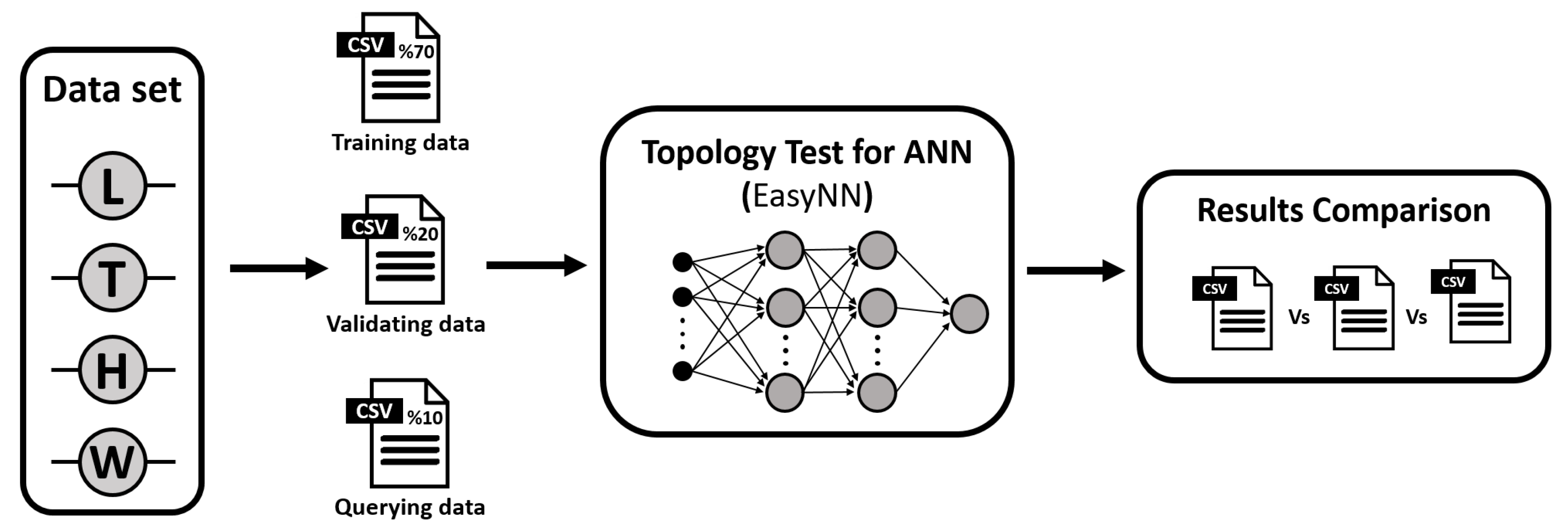
The dataset will undergo a systematic partitioning procedure, creating three distinct datasets: the training, validation, and testing datasets. Each dataset’s designated role in the modeling process corresponds to its nomenclature. To compose these datasets, instances will be randomly selected from the initial set of 1000 instances. Particularly, the training dataset will encompass 70% of the data, while the validation dataset will comprise 20%, and the remaining 10% will form the querying dataset. Subsequently, these datasets will be subjected to an array of neural network topologies as part of an extensive comparative analysis. Please refer to
Figure 8 for a graphical representation clarifying the neural network’s training methodology.
During training, data are passed forward through the neural network in what is known as feed-forward. Each layer performs calculations based on the weights, biases, and activation functions defined in the topology. The resulting predictions are compared to the actual target power values, and an error (typically mean squared error for regression tasks) is calculated. The feed-forward process considers the dataset previously normalized and randomly organized. Then, any possible errors in estimations are improved by applying the backpropagation process.
This involves calculating the error gradient with respect to the network’s weights and biases. This gradient information is then used to update the weights and biases through optimization algorithms like stochastic gradient descent (SGD), Adam, or RMSprop. These updates are performed iteratively for multiple epochs until the model converges to a satisfactory performance level. For this research, the authors used the Adam algorithm.
The combination of feed-forward and backpropagation for each instance is the core of the training process. The aforementioned procedure is subsequently executed on the complete training dataset. It is repeated for the number of epochs specified for each topology with their respective hyper-parameters for the Adam algorithm [
31].
4. Discussion and Conclusions
The significance of establishing the optimal neural network topology is highlighted by its dependence on input variables and their respective correlations. A series of models were trained, featuring a variety of input variable combinations, neuron quantities, and hidden layer configurations, with the overarching objective of identifying the most proficient model for the purposes of regression and forecasting. Nonetheless, certain limitations are inherent in the designed IoT prototype, encompassing aspects such as measurement resolution and ranges. Consequently, an evaluation was conducted to gauge the accuracy of the values derived from the IoT device. This evaluation involved a comparative analysis between the data generated by the prototype and those originating from a commercial meteorological station. After the computation of the root mean square error (RMSE) value, it was deduced that the data generated by our prototype exhibit reliability.
The presented methodology offers a comprehensive procedure for developing and utilizing artificial neural networks (ANNs) as regressors in conjunction with a measurement Internet of Things (IoT) device. This methodology can be applied further to larger photovoltaic (PV) systems or include more measurement variables. The data sets were prepared in Matlab®, and the model’s training process was implemented using EasyNN-plus software version V8, created by Neural Planner Software Ltd., from Cheadle, the United Kingdom.
Data have been partitioned into three key datasets: training (70% of the data), validation (20%), and querying or testing (10%). These sets were derived from an initial pool of 1000 instances. Then, training sets were processed through various neural network topologies for in-depth comparison. During the neural network training, data undergo a feed-forward process. Next, predictions made with the testing set are compared to target values to calculate errors.
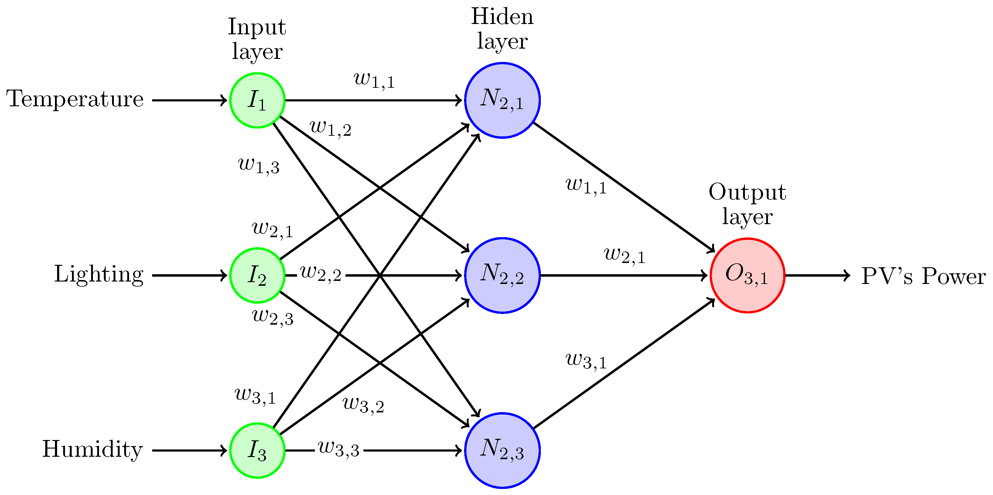
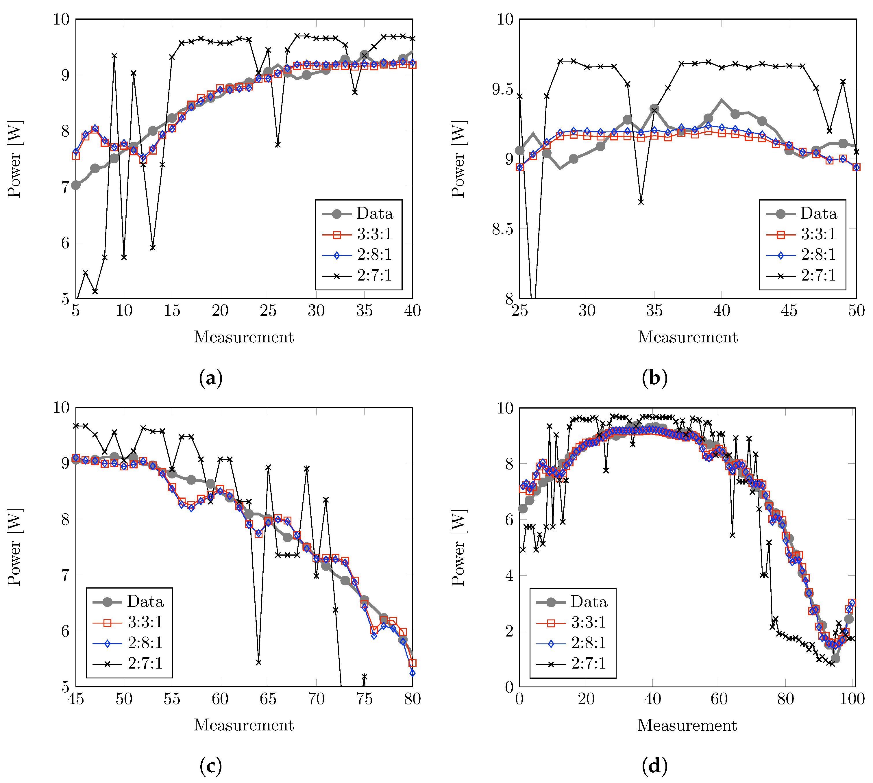
The most suitable configuration allows for accurate power estimates of the modeling PV panel. After prudent analysis, it has been determined that the optimal topology for this regression task consists of three main variables as inputs, three computational elements in the hidden layers, and one element in the output layer (3:3:1). The ANNs’ weight and bias parameters were obtained after training diverse models that consider different input variables and ANN topologies. By utilizing the 3:3:1 topology, it is possible to accurately predict the behavior of the solar panel under normal conditions with an RMSE performance of 0.2553 or 2.8%. Even with the two-variable model (2:8:1), there is only a slight margin of error, with a reliability level of 0.2730 or 3.03%. However, this model must be used with caution because estimations are made without lighting information. It is important to note that two-variable models have a significant drawback when considering the humidity variable, consistently resulting in the highest root mean square error (RMSE) values compared to other models. The elevated RMSE values indicate a substantial difference between the predicted and observed values, suggesting that placing excessive focus on humidity may not be the most optimal approach for accurate predictions in this scenario. Several factors could contribute to this outcome. Although crucial in many environmental and climatic studies, humidity might interact with other unaccounted variables that influence the prediction accuracy in this study. High RMSE values highlight the importance of considering a more diverse set of predictors or re-evaluating the weight assigned to humidity in the models.
Additionally, note that the models are trained and validated using clear-sky data, which is one of the limitations of this study. Nonetheless, the IoT system is continuously collecting fresh data to enhance the current findings and refine the models. Although the present outcomes offer a comprehensive understanding of the model’s abilities in specific conditions, it is imperative to investigate and fine-tune the model under different sky conditions, particularly in cloudy and overcast settings. This is a critical avenue for future research that will ultimately enhance the models’ precision and dependability.
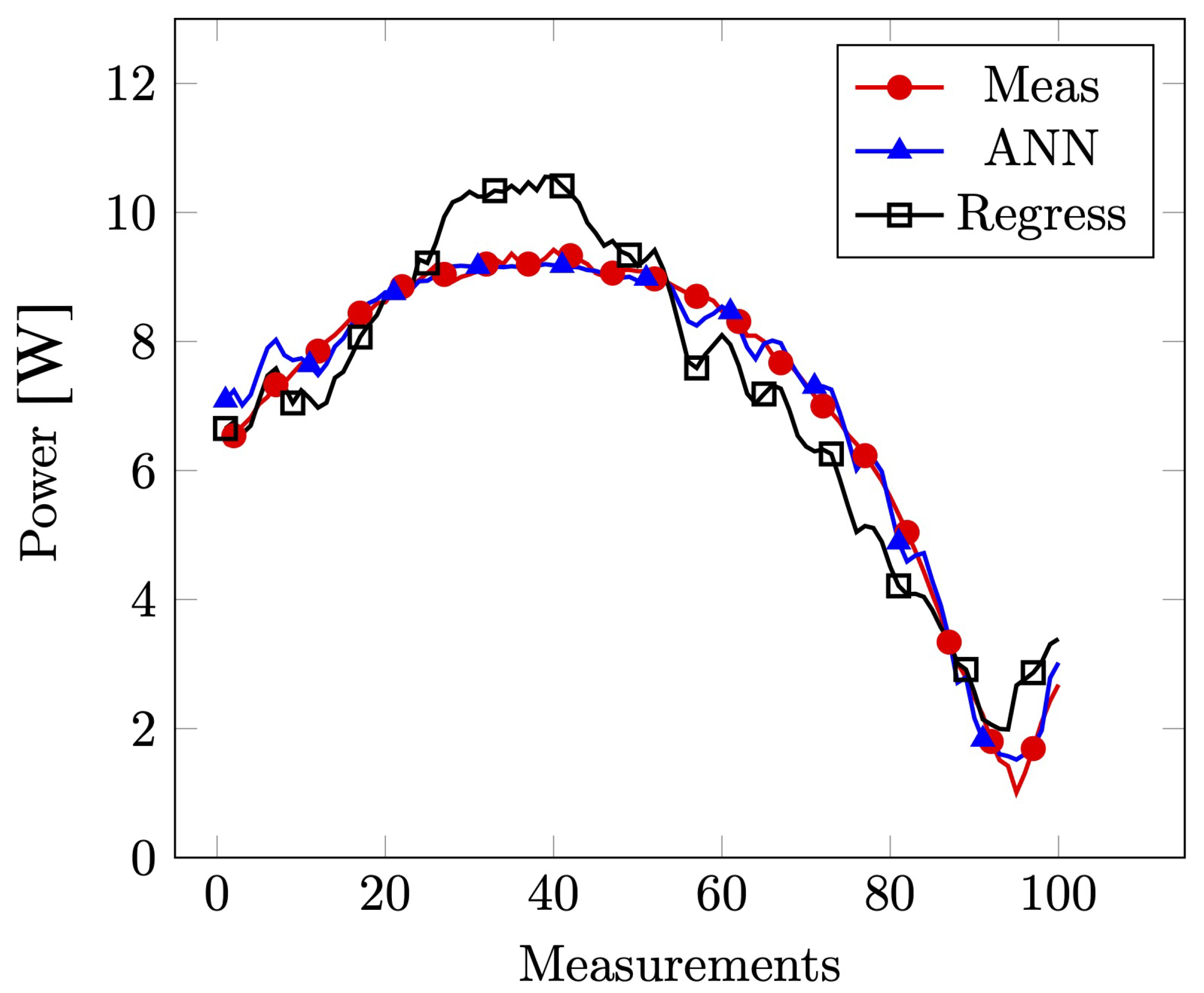
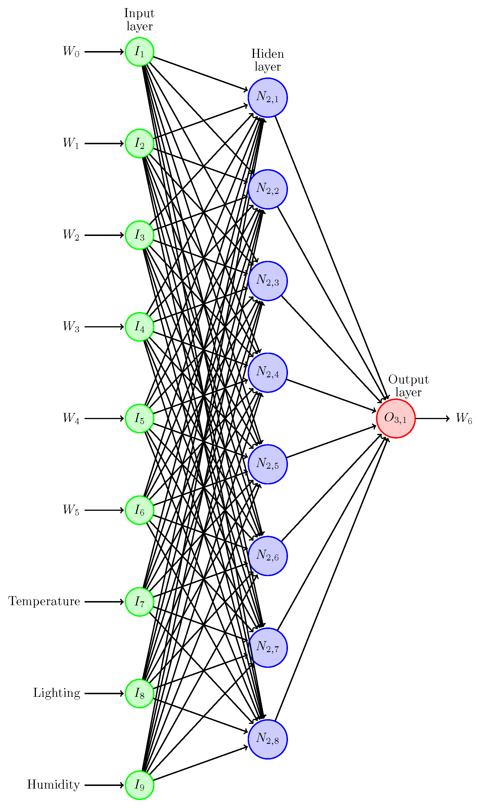
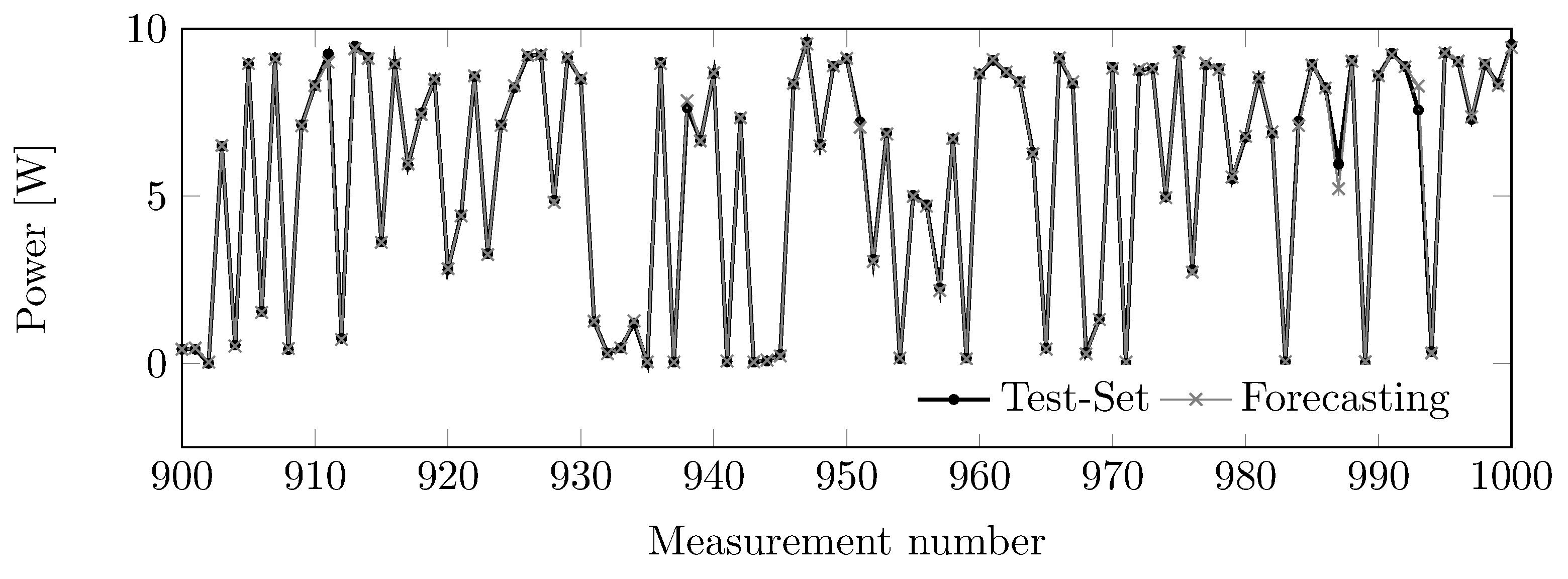
On the other hand, the forecasting model performs best with nine inputs: lighting, temperature, humidity, and six previous power values; the 9:9:1 topology. Next, eight nodes are in the hidden layer, and one node is in the output layer. The selected model is a non-autoregressive neural network (Non-AR-NN) that uses sequential data as input, together with actual environmental measurements.
The RMSE value forecasting predictions confirms that it is possible to make accurate estimates using the lighting, temperature, and humidity data next to the PV system. Forthcoming work will develop a more comprehensive multi-layer ANN model that considers larger datasets from on-site measurements. Also, more complex forecasting models can be developed using recurrent neural networks, autoregressive models, or medium-term models. Finally, the Internet of Things (IoT) accuracy can be improved and tested with larger systems.

 ,
, 


