
A Two-Dimensional K-Shell X-ray Fluorescence (2D-KXRF) Model for Soft Tissue Attenuation Corrections of Strontium Measurements in a Cortical Lamb Bone Sample


Abstract
:1. Introduction
2. Materials and Methods
2.1. KXRF Lamb Bone Sr Measurements
2.1.1. Experimental Setup
2.1.2. Experimental Samples
2.1.3. XRF Experimental Procedures
2.1.4. Data Analysis
2.2. X-ray Linear Attenuation Coefficient Measurements
2.3. 2D-KXRF Model
2.3.1. Theory
2.3.2. Numerical Implementation
3. Results
3.1. XRF Measurements
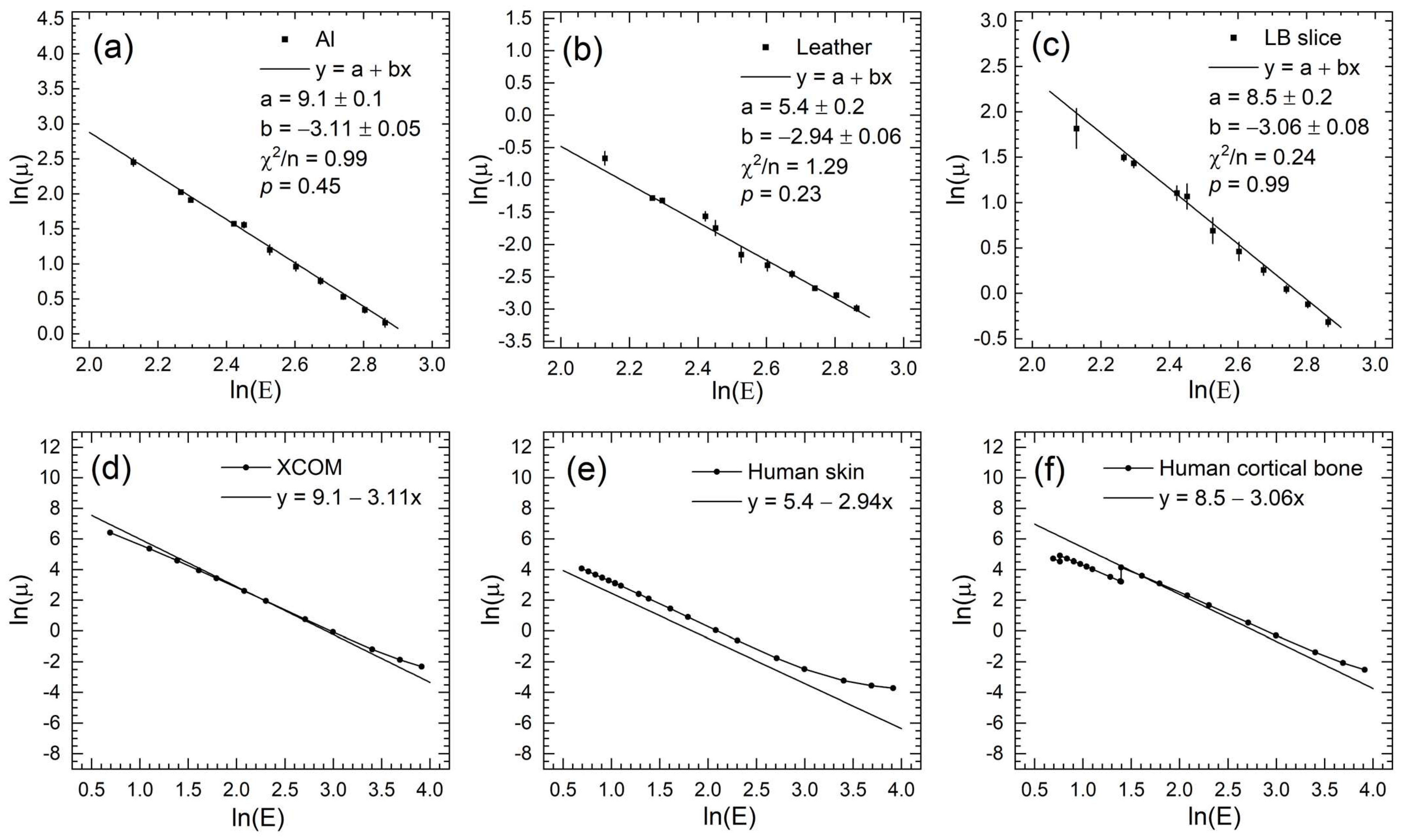
3.2. Linear Attenuation Coefficients Measurements
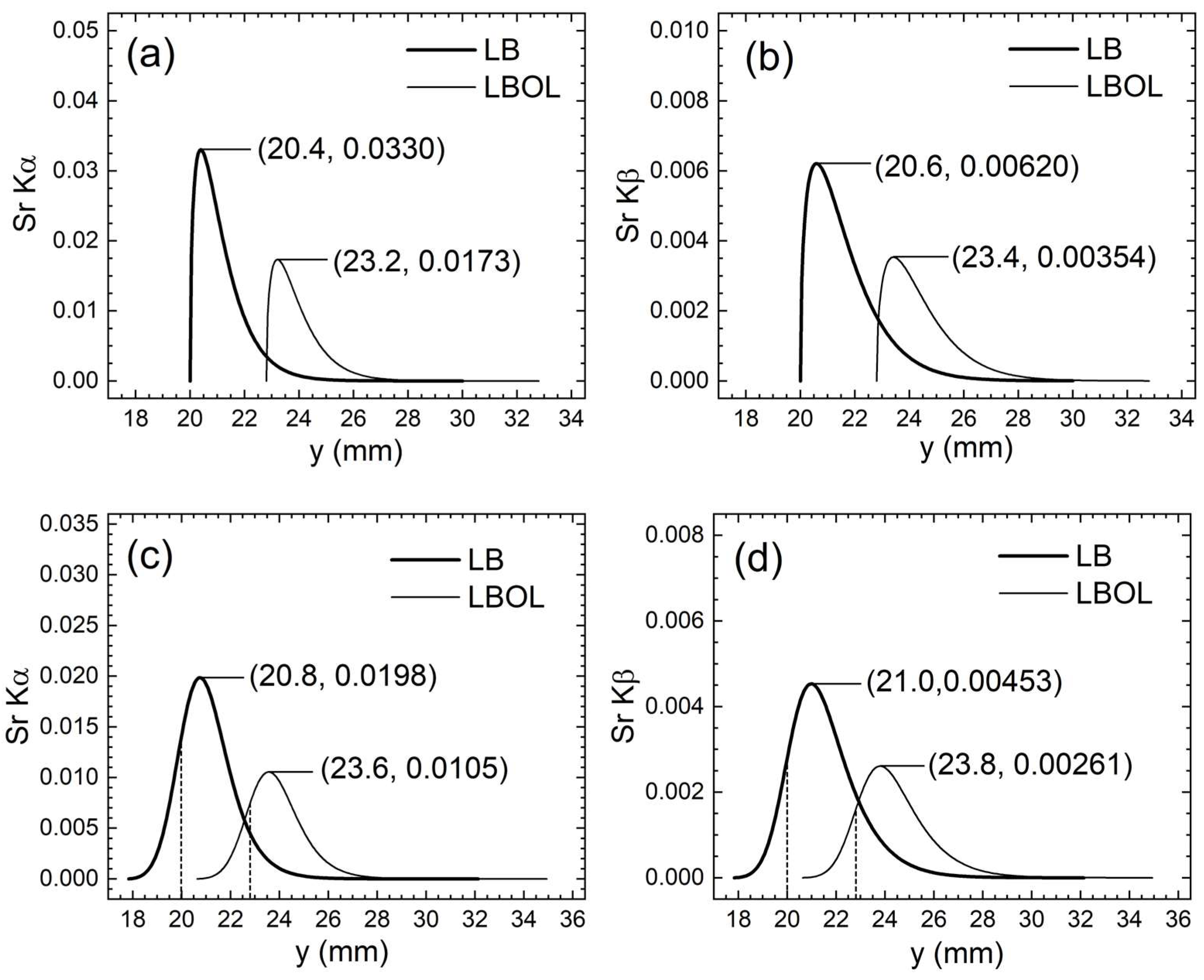
3.3. 2D-KXRF Model Output
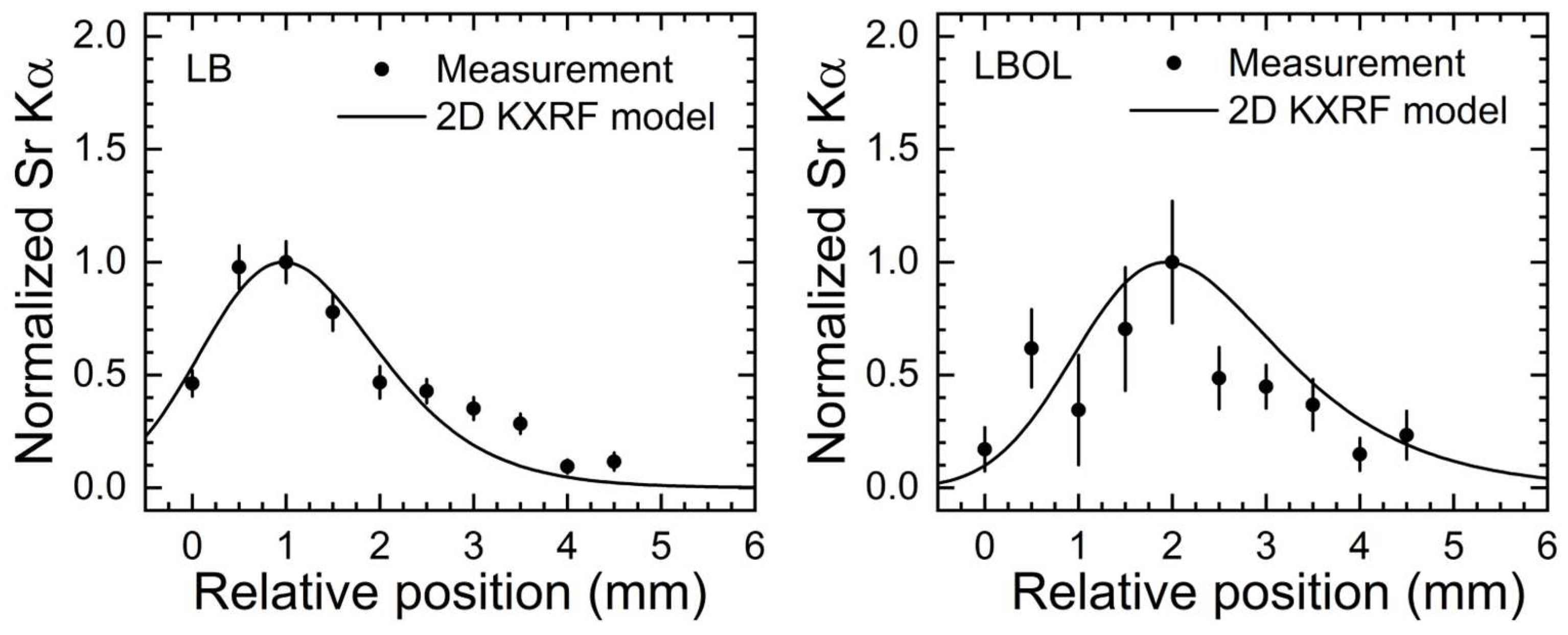
3.4. Comparison between 2D-KXRF Model and Experimental Results
3.5. Sr Concentration Estimates
4. Discussion
5. Conclusions
Supplementary Materials
Funding
Data Availability Statement
Acknowledgments
Conflicts of Interest
Appendix A
References
- Hall, T. X-ray fluorescence analysis in biology. Science 1961, 134, 449–455. Available online: http://www.jstor.org/stable/1707782 (accessed on 22 May 2023). [CrossRef] [PubMed]
- Mattson, S.; Börjesson, J. X-ray fluorescence in medicine. Spectrosc. Eur./World 2008, 20, 15–17. [Google Scholar]
- Chettle, D.R.; McNeill, F.E. Elemental analysis in living human subjects using biomedical devices. Physiol. Meas. 2019, 40, 12TR01. [Google Scholar] [CrossRef] [PubMed]
- Deslattes, R.D.; Kessler, E.G.; Indelicato, P.; de Billy, L.; Lindroth, E.; Anton, J. X-ray transition energies: New approach to a comprehensive evaluation. Rev. Mod. Phys. 2003, 75, 35–90. [Google Scholar] [CrossRef]
- Malmstrom, B.G.; Neilands, J.B. Metalloproteins. Annu. Rev. Biochem. 1964, 33, 331–354. [Google Scholar] [CrossRef] [PubMed]
- Shi, W.; Chance, M.R. Metallomics and metalloproteomics. Cell. Mol. Life Sci. 2008, 65, 3040–3048. [Google Scholar] [CrossRef]
- Waldron, K.J.; Rutherford, J.C.; Ford, D.; Robinson, N.J. Metalloproteins and metals sensing. Nature 2009, 460, 823–830. [Google Scholar] [CrossRef]
- Hoffer, P.B.; Jones, W.B.; Crawford, W.B.; Beck, R.; Gottschalk, A. Fluorescent thyroid scanning: A new method of imaging the thyroid. Radiology 1968, 90, 342–344. [Google Scholar] [CrossRef]
- Ahlgren, L.; Lidén, K.; Mattson, S.; Tejning, S. X-ray fluorescence analysis of lead in human skeleton in vivo. Scand. J. Work. Environ. Health 1976, 2, 82–86. Available online: https://www.jstor.org/stable/40964582 (accessed on 29 September 2015). [CrossRef]
- Somervaille, L.J.; Chettle, D.R.; Scott, M.C. In vivo measurement of lead in bone using x-ray fluorescence. Phys. Med. Biol. 1985, 30, 929–943. [Google Scholar] [CrossRef]
- Keldani, Z.; Lord, M.L.; McNeill, F.E.; Chettle, D.R.; Gräfe, J.L. Coherent normalization for in vivo measurements of gadolinium in bone. Physiol. Meas. 2017, 38, 1848–1858. [Google Scholar] [CrossRef] [PubMed]
- Nie, H.; Chettle, D.; Luo, L.; O’Meara, J. In vivo investigation of a new 109Cd γ-ray induced K-XRF bone lead measurement system. Phys. Med. Biol. 2006, 51, 351–360. [Google Scholar] [CrossRef] [PubMed]
- Wielopolski, L.; Rosen, J.F.; Slatkin, D.N.; Vartsky, D.; Ellis, K.J.; Cohn, S.H. Feasibility of noninvasive analysis of lead in human tibia by soft x-ray fluorescence. Med. Phys. 1983, 10, 248–251. [Google Scholar] [CrossRef] [PubMed]
- Zamburlini, M.; Pejović-Milić, A.; Chettle, D.R. Coherent normalization of finger strontium XRF measurements: Feasibility and limitations. Phys. Med. Biol. 2008, 53, N307. [Google Scholar] [CrossRef] [PubMed]
- Nguyen, J.; Crawford, D.; Howarth, D.; Sukhu, B.; Pejović-Milić, A.; Gräfe, J.L. Ex vivo quantification of lanthanum and gadolinium in post-mortem human tibiae with estimated barium and iodine concentrations using K x-ray fluorescence. Physiol. Meas. 2019, 40, 085006. [Google Scholar] [CrossRef]
- Nguyen, J.; Pejović-Milić, A.; Gräfe, J.L. Investigating coherent normalization and dosimetry for the Am-La K XRF system. Physiol. Meas. 2020, 41, 075014. [Google Scholar] [CrossRef]
- Sherman, J. The theoretical derivation of fluorescent X-ray intensities from mixtures. Spectrochim. Acta 1955, 7, 283–306. [Google Scholar] [CrossRef]
- Van Dyck, P.M.; Török, S.B.; Van Grieken, R.E. Enhancement effect in x-ray fluorescence analysis of environmental samples of medium thickness. Anal. Chem. 1986, 58, 1761–1766. [Google Scholar] [CrossRef]
- Nielson, K.K. Matrix corrections for energy dispersive x-ray fluorescence analysis of environmental samples with coherent/incoherent scattered x-rays. Anal. Chem. 1977, 49, 641–648. [Google Scholar] [CrossRef]
- He, F.; Van Espen, P.J. General approach for quantitative energy dispersive x-ray fluorescence analysis based on fundamental parameters. Anal. Chem. 1991, 63, 2237–2244. [Google Scholar] [CrossRef]
- Sprang, V.; Bekkers, M.H.J. Determination of light elements using x-ray spectrometry. Part I—Analytical implications using scattered tube lines. X-ray Spectrom. 1998, 27, 31–36. [Google Scholar] [CrossRef]
- Wegrzynek, D.; Markowicz, A.; Chinea-Cano, E. Application of the backscattered fundamental parameter method for in situ element determination using a portable energy-dispersive x-ray fluorescence spectrometer. X-ray Spectrom. 2003, 32, 119–128. [Google Scholar] [CrossRef]
- Bos, M.; Vrielink, J.A.M. Constraints, iteration schemes and convergence criteria for concentration calculations in X-ray fluorescence spectrometry with the use of the fundamental parameter methods. Anal. Chim. Acta 1998, 373, 291–302. [Google Scholar] [CrossRef]
- Kitov, B.I. Calculation features of the fundamental parameter method in XRF. X-ray Spectrom. 2000, 29, 285–290. [Google Scholar] [CrossRef]
- Szalóki, I.; Gerényi, A.; Radócz, G.; Lovas, A.; De Samber, B.; Vincze, L. FPM model calculation for micro X-ray fluorescence confocal imaging using synchrotron radiation. J. Anal. At. Spectrom. 2017, 32, 334–344. [Google Scholar] [CrossRef]
- Malzer, W.; Kanngießer, B. Calculation of attenuation and X-ray fluorescence intensities for non-parallel x-ray beams. X-ray Spectrom. 2003, 32, 106–112. [Google Scholar] [CrossRef]
- Vasquez, R.P. Composition determination for complex and transmitting samples in x-ray quantitative analysis. X-ray Spectrom. 2008, 37, 599–602. [Google Scholar] [CrossRef]
- Barrea, R.A.; Bengió, S.; Derosa, P.A.; Mainardi, R.T. Absolute mass thickness determination of thin samples by X-ray fluorescence analysis. Nucl. Instrum. Methods Phys. Res. B 1998, 143, 561–568. [Google Scholar] [CrossRef]
- Fiorini, C.; Gianoncelli, A.; Longoni, A.; Zaraga, F. Determination of the thickness of coatings by means of a new XRF spectrometer. X-ray Spectrom. 2002, 31, 92–99. [Google Scholar] [CrossRef]
- Nygård, K.; Hämäläinen, K.; Manninen, S.; Jalas, P.; Ruottinen, J.-P. Quantitative thickness determination using x-ray fluorescence: Application to multiple layers. X-ray Spectrom. 2004, 33, 354–359. [Google Scholar] [CrossRef]
- De Boer, D.K.G. Calculation of x-ray fluorescence intensities from bulk and multilayer samples. X-ray Spectrom. 1990, 19, 145–154. [Google Scholar] [CrossRef]
- De Boer, D.K.G.; Borstrok, J.J.M.; Leenaers, A.J.G.; Van Sprang, H.A. How accurate is the fundamental parameter approach? XRF analysis of bulk and multilayer samples. X-ray Spectrom. 1993, 22, 33–38. [Google Scholar] [CrossRef]
- Gherase, M.R.; Fleming, D.E.B. Calculation of depth-dependent elemental concentration with X-ray fluorescence using a layered calibration method. Nucl. Instrum. Methods Phys. Res. B 2011, 269, 1150–1156. [Google Scholar] [CrossRef]
- Todd, A.C.; Chettle, D.R.; Scott, M.C.; Somervaille, L.J. Monte Carlo modelling of in vivo x-ray fluorescence of lead in the kidney. Phys. Med. Biol. 1991, 36, 439–448. [Google Scholar] [CrossRef]
- Tartari, A.; Fernandez, J.E.; Casnati, E.; Baraldi, C.; Felsteiner, J. EDXRS modelling for in vivo trace element analysis by using the SHAPE code. X-ray Spectrom. 1993, 22, 323–327. [Google Scholar] [CrossRef]
- Vincze, L.; Janssen, K.; Adams, F.; Rivers, M.L.; Jones, K.W. A general Monte Carlo simulation of energy dispersive X-ray fluorescence spectrometers—I: Unpolarized radiation, homogeneous samples. Spectrochim. Acta 1993, 48, 553–573. [Google Scholar] [CrossRef]
- Wallace, J.D. The Monte Carlo modelling of in vivo x-ray fluorescence measurement of lead in tissue. Phys. Med. Biol. 1994, 39, 1745–1756. [Google Scholar] [CrossRef]
- Vincze, L.; Janssen, K.; Adams, F. A general Monte Carlo simulation of energy dispersive X-ray fluorescence spectrometers. II: Polarized monochromatic radiation, homogeneous samples. Spectrochim. Acta B 1995, 50, 127–147. [Google Scholar] [CrossRef]
- Vincze, L.; Janssen, K.; Adams, F. A general Monte Carlo simulation of energy dispersive X-ray fluorescence spectrometers. Part 3. Polarized polychromatic radiation, homogeneous samples. Spectrochim. Acta B 1995, 50, 1481–1500. [Google Scholar] [CrossRef]
- Ao, Q.; Lee, S.H.; Gardner, R.P. Development of the specific purpose Monte Carlo CEARXRF for the design and use of in vivo x-ray fluorescence analysis systems for lead in bone. Appl. Radiat. Isot. 1997, 48, 1403–1412. [Google Scholar] [CrossRef]
- O’Meara, J.M.; Chettle, D.R.; McNeill, F.E.; Prestwich, W.V.; Svensson, C.E. Monte Carlo simulation of source-excited in vivo x-ray fluorescence measurements of heavy metals. Phys. Med. Biol. 1998, 43, 1413–1428. [Google Scholar] [CrossRef] [PubMed]
- Vincze, L.; Janssen, K.; Vekemans, B.; Adams, F. Monte Carlo simulation of X-ray fluorescence spectra. Part 4. Photon scattering at high X-ray energies. Spectrochim. Acta B 1999, 54, 1711–1722. [Google Scholar] [CrossRef]
- Guo, W.; Gardner, R.P.; Todd, A.C. Using the Monte Carlo—Library least-Squares (MCLLS) approach for the in vivo XRF measurement of lead in bone. Nucl. Instrum. Meth. Phys. Res. A 2004, 516, 586–593. [Google Scholar] [CrossRef]
- Zamburlini, M.; Byun, S.H.; Pejović-Milić, B.A.; Prestwich, W.V.; Chettle, D.R. Evaluation of MCNP5 and EGS4 for the simulation of in vivo strontium XRF measurements. X-ray Spectrom. 2007, 36, 76–81. [Google Scholar] [CrossRef]
- Hodoroaba, V.D.; Radtke, M.; Vincze, L.; Rackwitz, V.; Reuter, D. X-ray scattering in X-ray fluorescence spectra with X-ray tube excitation—Modelling, experiment, and Monte-Carlo simulation. Nucl. Instrum. Meth. Phys. Res. B 2010, 268, 3568–3575. [Google Scholar] [CrossRef]
- Schoonjans, T.; Solé, V.A.; Vincze, L.; del Rio, M.S.; Brondeel, P.; Silversmit, G.; Appel, K.; Ferrero, C. A general Monte Carlo simulation of energy-dispersive X-ray fluorescence spectrometers—Part 5. Polarized radiation, stratified samples, cascade effects, M-lines. Spectrochim. Acta B 2012, 70, 10–23. [Google Scholar] [CrossRef]
- Schoonjans, T.; Solé, V.A.; Vincze, L.; del Rio, M.S.; Appel, K.; Ferrero, C. A general Monte Carlo simulation of energy-dispersive X-ray fluorescence spectrometers—Part 6. Quantification through iterative simulations. Spectrochim. Acta B 2013, 82, 36–41. [Google Scholar] [CrossRef]
- Scot, V.; Fernandez, J.E. The Monte Carlo code MCSHAPE: Main features and recent developments. Spectrochim. Acta B 2015, 108, 53–60. [Google Scholar] [CrossRef]
- Sharma, U.; Van Delinder, K.; Gräfe, J.L.; Fleming, D.E.B. Investigating methods of normalization for X-ray fluorescence measurements of zinc in nail clippings using the TOPAS Monte Carlo code. Appl. Radiat. Isot. 2022, 182, 110151. [Google Scholar] [CrossRef]
- Fernández, J.E. XRF intensity in the frame of the transport theory. X-ray Spectrom. 1989, 18, 271–279. [Google Scholar] [CrossRef]
- Fernández, J.E. Polarization effects in multiple scattering photon calculations using the Boltzmann vector equation. Radiat. Phys. Chem. 1999, 56, 27–59. [Google Scholar] [CrossRef]
- Fernández, J.E. Analysis of the effects of geometry on the fluorescence radiation field in the frame of transport theory. X-ray Spectrom. 2005, 34, 7–10. [Google Scholar] [CrossRef]
- Fernández, J.E. Multiple scattering of photons using the Boltzmann transport equation. Nucl. Instrum. Meth. Phys. Res. B 2007, 263, 7–21. [Google Scholar] [CrossRef]
- Fernández, J.E.; Teodori, F. Major and minor contributions to X-ray characteristic lines in the framework of the Boltzmann transport equation. Quantum Beam Sci. 2022, 6, 20. [Google Scholar] [CrossRef]
- Andreo, P. Monte Carlo techniques in medical radiation physics. Phys. Med. Biol. 1991, 36, 861–920. [Google Scholar] [CrossRef]
- Rogers, D.W.O. Fifty years of Monte Carlo simulations for medical physics. Phys. Med. Biol. 2006, 51, R287–R301. [Google Scholar] [CrossRef] [PubMed]
- Rogers, D.W.O. Reflections on a life with Monte Carlo in Medical Physics. Med. Phys. 2023, 50, 91–94. [Google Scholar] [CrossRef] [PubMed]
- Gherase, M.R.; Al-Hamdani, S. A microbeam grazing-incidence approach to L-shell x-ray fluorescence measurements of lead concentration in bone and soft tissue phantoms. Physiol. Meas. 2018, 39, 035007. [Google Scholar] [CrossRef] [PubMed]
- Gherase, M.R.; Al-Hamdani, S. Improvements and reproducibility of an optimal grazing-incidence position method to L-shell x-ray fluorescence measurements of lead in bone and soft tissue phantoms. Biomed. Phys. Eng. Express 2018, 4, 065024. [Google Scholar] [CrossRef] [PubMed]
- Gherase, M.R.; Blaz, S.; Kroeker, S. A novel calibration for L-shell x-ray fluorescence measurements of bone lead concentration using the strontium Kβ/Kα ratio. Physiol. Meas. 2021, 42, 045011. [Google Scholar] [CrossRef]
- Gherase, M.R.; Vargas, A.F. Effective X-ray beam size measurements of an X-ray tube and polycapillary X-ray lens system using a scanning X-ray fluorescence method. Nucl. Instrum. Meth. Phys. Res. B 2017, 395, 5–12. [Google Scholar] [CrossRef]
- Mairs, S.; Swift, B.; Rutty, G.N. Detergent. An alternative approach to traditional bone cleaning methods for forensic practice. Am. J. Forensic Med. Pathol. 2004, 25, 276–284. [Google Scholar] [CrossRef] [PubMed]
- Berger, M.J.; Hubbell, J.H.; Seltzer, S.M.; Chang, J.; Sukumar, R.; Zucker, D.S.; Olsen, K. XCOM: Photon Cross Section Database, Version 1.5; National Institute of Standards and Technology: Gaithersburg, MD, USA, 2010. [Google Scholar]
- Elam, W.T.; Ravel, B.D.; Sieber, J.R. A new atomic database for X-ray spectroscopic calculations. Radiat. Phys. Chem. 2002, 63, 121–128. [Google Scholar] [CrossRef]
- Press, W.H.; Teukolsky, S.A.; Vetterling, W.T.; Flannery, B.P. Numerical Recipes, 3rd ed.; Cambridge University Press: New York, NY, USA, 2007; pp. 120–124. [Google Scholar]
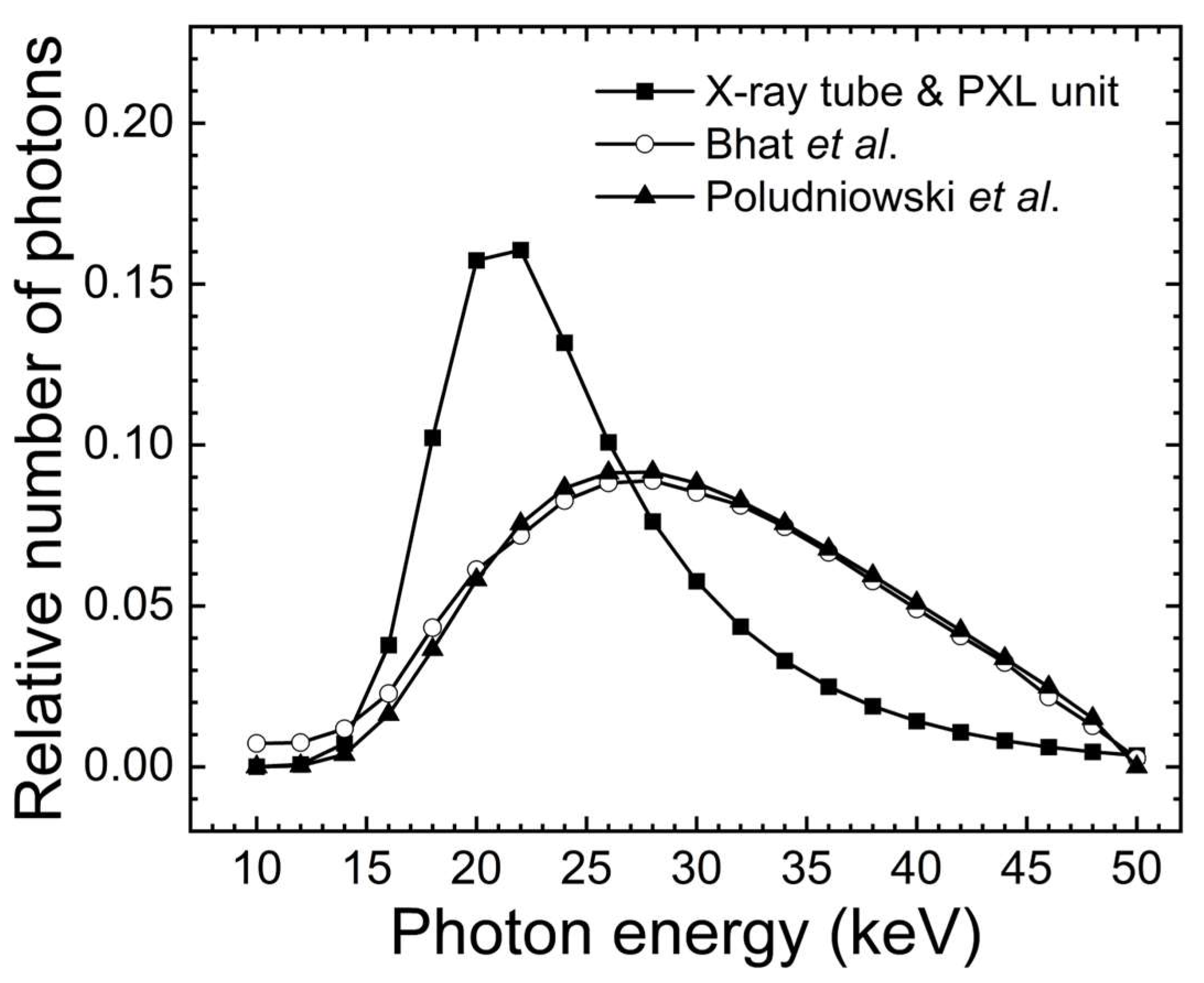
- Kroeker, S.E. Energy Spectrum and Exposure Measurements of an X-ray Tube and PXL Produced Microbeam Used in Bone Lead XRF Studies. Master’s Thesis, California State University, Fresno, CA, USA, 2021. [Google Scholar]
- Bhat, M.; Pattison, J.; Bibbo, G.; Caon, M. Diagnostic x-ray spectra: A comparison of spectra generated by different computational methods with a measured spectrum. Med. Phys. 1998, 25, 114–120. [Google Scholar] [CrossRef] [PubMed]
- Poludniowski, G.; Landry, G.; DeBlois, F.; Evans, P.M.; Verhaegen, F. SpekCalc: A program to calculate spectra from tungsten anode x-ray tubes. Phys. Med. Biol. 2009, 54, N433–N438. [Google Scholar] [CrossRef] [PubMed]
- MacDonald, C.A.; Gibson, W.M. Applications and advances in polycapillary optics. X-ray Spectrom. 2003, 32, 258–268. [Google Scholar] [CrossRef]
- ICRU. Tissue Substitutes in Radiation Dosimetry and Measurement; Report 44; International Commission on Radiation Units and Measurements: Bethesda, MD, USA, 1989; p. 22. [Google Scholar]
- Zhou, H.; Keall, P.J.; Graves, E.E. A bone composition model for Monte Carlo x-ray transport simulations. Med. Phys. 2009, 36, 1008–1018. [Google Scholar] [CrossRef]
- Taylor, J.R. An introduction to error analysis. In The Study of Uncertainties in Physical Measurements, 2nd ed.; University Science Books: Sausalito, CA, USA, 1997; pp. 73–77. [Google Scholar]
- Ertuğral, B.; Apaydin, G.; Çevik, U.; Ertuğrul, M.; Kobya, A.I. Kβ/Kα X-ray intensity ratios for elements in the range 16 ≤ Z ≤ 92 excited by 5.9, 59.5 and 123.6 keV photons. Radiat. Phys. Chem. 2007, 76, 15–22. [Google Scholar] [CrossRef]
- Pejović-Milić, A.; Stronach, I.M.; Gyorffy, J.; Webber, C.E.; Chettle, D.R. Quantification of bone strontium level in humans by in vivo x-ray fluorescence. Med. Phys. 2004, 31, 528–538. [Google Scholar] [CrossRef]
- Zamburlini, M.; Campbell, J.L.; de Silveira, G.; Butler, R.; Pejović-Milić, A.; Chettle, D.R. Strontium depth distribution in human bone measured by micro-PIXE. X-ray Spectrom. 2009, 38, 271–277. [Google Scholar] [CrossRef]
- Möhring, S.; Cieplik, F.; Hiller, K.-A.; Ebensberger, H.; Ferstl, G.; Hermens, J.; Zaparty, M.; Witzgall, R.; Mansfeld, U.; Buchalla, W.; et al. Elemental compositions of enamel or dentin in human and bovine teeth differ from murine teeth. Materials 2023, 16, 1514. [Google Scholar] [CrossRef] [PubMed]


| Symbol | Significance | Value/Range | Units | Source |
|---|---|---|---|---|
| Incident photon energy | 10–50 | keV | Measurement | |
| Average Kα photon energy | 14.1 | keV | Deslattes et al. [4] | |
| Average Kβ photon energy | 15.8 | keV | Deslattes et al. [4] | |
| Mass density of cortical bone | 1.9 | g cm−3 | ||
| Sr photoelectric mass attenuation coefficient at photon energy | 60.65–49.70 | cm2 g−1 | XCOM database [64] | |
| K-shell vacancy probability for Sr | 0.8548 | - | Elam et al. [64] | |
| K-shell fluorescence yield | 0.6647 | - | Elam et al. [64] | |
| Relative Kα emission intensity | 0.8488 | - | Elam et al. [64] | |
| Relative Kβ emission intensity | 0.1512 | - | Elam et al. [64] | |
| Soft tissue linear attenuation coefficient at photon energies , , and . | variable | mm−1 | Measurement | |
| Bone linear attenuation coefficient at photon energies and . | variable | mm−1 | Measurement and XCOM database | |
| Beryllium (Be) linear attenuation coefficient at photon energy . | variable | cm−1 | XCOM database and Be density: 1.85 g cm−3 | |
| Silicon (Si) linear attenuation coefficient at photon energy . | variable | cm−1 | XCOM database and Si density: 1.85 g cm−3 | |
| Be detector window thickness | 0.00125 | cm | Manufacturer | |
| Si detector thickness | 0.05 | cm | Manufacturer |
| 10 | 24 | 38 | |||
| 12 | 26 | 40 | |||
| 14 | 28 | 42 | |||
| 16 | 30 | 44 | |||
| 18 | 32 | 46 | |||
| 20 | 34 | 48 | |||
| 22 | 36 | 50 |
| LB | LBOL | ||
|---|---|---|---|
| XRF Peak | Peak Area | XRF Peak | Peak Area |
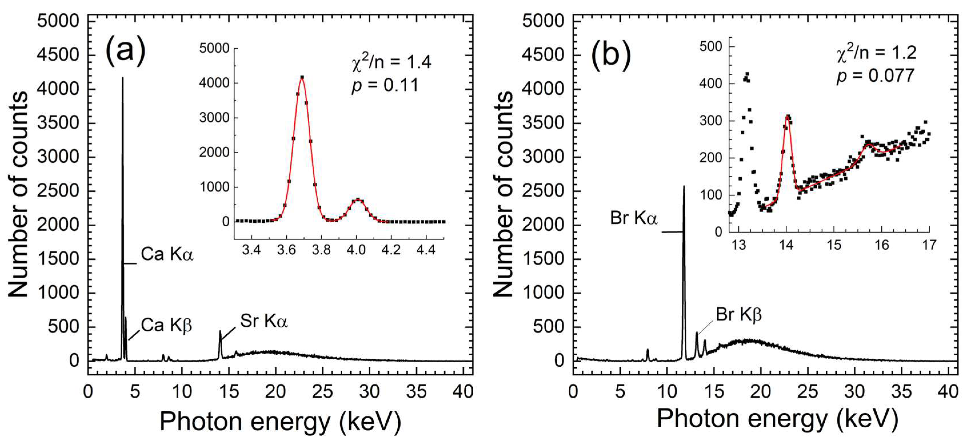
| P Kα | 11.3 ± 0.5 | Zn Kα | 3.3 ± 0.2 |
| S Kα | 2.1 ± 0.4 | Zn Kβ | 0.7 ± 0.1 |
| K Kα | 0.9 ± 0.4 | Br Kα | 518 ± 3 |
| Ca Kα | 475 ± 2 | Br Kβ | 81 ± 1 |
| Ca Kβ | 77.9 ± 0.9 | Sr Kα | 49 ± 1 |
| Zn Kα | 10.8 ± 0.3 | Sr Kβ | 10 ± 1 |
| Zn Kβ | 1.8 ± 0.2 | ||
| Sr Kα | 89 ± 1 | ||
| Sr Kβ | 15.1 ± 0.8 | ||
| Sample | y-Axis Position (mm) | X-ray Photon | X-ray Beam | ||
|---|---|---|---|---|---|
| Sr Kα | Sr Kβ | Sr Kα | Sr Kβ | ||
| LB | 20.0 | 0.0000 (edge) | 0.00000 (edge) | 0.0140 (edge) | 0.00275 (edge) |
| 20.4 | 0.0330 (max) | 0.00602 | 0.0185 | 0.00387 | |
| 20.6 | 0.0313 | 0.00620 (max) | 0.0196 | 0.00425 | |
| 20.8 | 0.0280 | 0.00605 | 0.0198 (max) | 0.00446 | |
| 21.0 | 0.0240 | 0.00571 | 0.0193 | 0.00453 (max) | |
| LBOL | 22.8 | 0.0000 (edge) | 0.0000 (edge) | 0.00748 (edge) | 0.00161 (edge) |
| 23.2 | 0.0173 (max) | 0.00341 | 0.00980 | 0.00220 | |
| 23.4 | 0.0165 | 0.00354 (max) | 0.0104 | 0.00242 | |
| 23.6 | 0.0151 | 0.00346 | 0.0106 (max) | 0.00256 | |
| 23.8 | 0.0130 | 0.00328 | 0.0103 | 0.00261 (max) | |
| Sample | Sr Kα | Sr Kβ | ||||
|---|---|---|---|---|---|---|
| Measurement | 2D-KXRF Model | Measurement | 2D-KXRF Model | |||
| LBOL | 49± 1 | 0.0106 | 10 ± 1 | 0.00256 | ||
| LB | 89 ± 1 | 0.0198 | 15.1 ± 0.8 | 0.00446 | ||
| LBOL/LB | 0.55 ± 0.01 | 0.535 | 0.772 ± 0.004 | 0.66 ± 0.07 | 0.574 | 0.831 ± 0.003 |
| Sample | (Sr Kβ/Kα)exp | ε(Kα)/ε(Kβ) | (Sr Kβ/Kα)exp·ε(Kα)/ε(Kβ) | Model |
|---|---|---|---|---|
| LB | 0.170 ± 0.009 | 1.19965 | 0.20 ± 0.01 | 0.225 |
| LBOL | 0.20 ± 0.02 | 1.19965 | 0.24 ± 0.02 | 0.240 |
| Sample | c (g g−1) | |||
|---|---|---|---|---|
| LB | 0.0198 | |||
| LBOL | 0.0106 | |||
| Sample | ||||
| LB | 0.00446 | |||
| LBOL | 0.00256 |
Disclaimer/Publisher’s Note: The statements, opinions and data contained in all publications are solely those of the individual author(s) and contributor(s) and not of MDPI and/or the editor(s). MDPI and/or the editor(s) disclaim responsibility for any injury to people or property resulting from any ideas, methods, instructions or products referred to in the content. |
© 2023 by the author. Licensee MDPI, Basel, Switzerland. This article is an open access article distributed under the terms and conditions of the Creative Commons Attribution (CC BY) license (https://creativecommons.org/licenses/by/4.0/).
Share and Cite
Gherase, M.R. A Two-Dimensional K-Shell X-ray Fluorescence (2D-KXRF) Model for Soft Tissue Attenuation Corrections of Strontium Measurements in a Cortical Lamb Bone Sample. Metrology 2023, 3, 325-346. https://doi.org/10.3390/metrology3040020
Gherase MR. A Two-Dimensional K-Shell X-ray Fluorescence (2D-KXRF) Model for Soft Tissue Attenuation Corrections of Strontium Measurements in a Cortical Lamb Bone Sample. Metrology. 2023; 3(4):325-346. https://doi.org/10.3390/metrology3040020
Chicago/Turabian StyleGherase, Mihai R. 2023. "A Two-Dimensional K-Shell X-ray Fluorescence (2D-KXRF) Model for Soft Tissue Attenuation Corrections of Strontium Measurements in a Cortical Lamb Bone Sample" Metrology 3, no. 4: 325-346. https://doi.org/10.3390/metrology3040020