Article

Inverse Problems in Pump–Probe Spectroscopy

1
Deutsches Elektronen-Synchrotron DESY, Notkestr. 85, 22607 Hamburg, Germany
2
Institute of Physical Chemistry, Christian-Albrechts-Universität zu Kiel, 24118 Kiel, Germany
*
Author to whom correspondence should be addressed.
Photochem 2024, 4(1), 57-110; https://doi.org/10.3390/photochem4010005
Submission received: 26 December 2023 / Revised: 17 January 2024 / Accepted: 19 January 2024 / Published: 31 January 2024
(This article belongs to the Special Issue Feature Papers in Photochemistry II)

Abstract

:
Ultrafast pump–probe spectroscopic studies allow for deep insights into the mechanisms and timescales of photophysical and photochemical processes. Extracting valuable information from these studies, such as reactive intermediates’ lifetimes and coherent oscillation frequencies, is an example of the inverse problems of chemical kinetics. This article describes a consistent approach for solving this inverse problem that avoids the common obstacles of simple least-squares fitting that can lead to unreliable results. The presented approach is based on the regularized Markov Chain Monte-Carlo sampling for the strongly nonlinear parameters, allowing for a straightforward solution of the ill-posed nonlinear inverse problem. The software to implement the described fitting routine is introduced and the numerical examples of its application are given. We will also touch on critical experimental parameters, such as the temporal overlap of pulses and cross-correlation time and their connection to the minimal reachable time resolution.

1. Introduction

Pump–probe spectroscopy is a powerful tool in the investigation of ultrafast kinetics [1]. The basic scheme of pump–probe studies is the following [1]. First, we initiate the system’s dynamics with a pump laser pulse, then wait some time for the excited molecular system to evolve, and then with a second probe laser pulse, we turn otherwise unobservable (due to their short lifetimes) metastable species into something new and observable by the detectors. By varying the delay time between pump and probe pulses (so-called pump–probe delay), we can measure the real-time photochemical dynamics of the molecules. Under the umbrella term “pump–probe spectroscopy”, multiple experimental methods hide that differ by what kind of observable is being monitored in the experiment [1,2,3,4]. The measured experimental parameters can be the absorption of the probe photons [5], mass spectra [6,7,8], photoelectron spectra [6,9], ion velocity map imaging [6,7,10], fluorescence [11], and so on [2,3]. We can extract viable information about the rates of various molecular processes from these pump–probe experimental results. To do that, we need to perform the experimental data analysis, which is at the center of this article.
The current manuscript presents a novel approach and its software implementation for performing such data analysis. It is based on mixed linear and nonlinear optimization [12], Monte-Carlo sampling [13,14], and regularization of fitting parameters [15,16,17], solving many issues of the ill-posed inverse problem of pump–probe experimental data analysis. First, we will formally examine the basic experimental data analysis and the least-squares fitting. Then, we will discuss the model of the pump–probe spectroscopy. This will be followed by a detailed description of the proposed data analysis algorithm and a short description of the implementation of such a method. In the end, a few numerical examples will be given. In the electronic supporting information (ESI), we also provide a user manual, an up-to-date software version, and the numerical examples described in the last section of this article.

2. Inverse Problem of Experimental Data Analysis

2.1. Formulation of the Problem

We can consider the following set of concepts to formalize the experimental data analysis treatment [14,16]. The experimental results are always interpreted through the prism of a model ( M ) that presents a concise and simplistic way to explain whatever happens in the experiment. In our case of pump–probe spectroscopy, it is the interaction of the observed molecular system with the pump and probe pulses, the internal dynamics of the molecule, and the production of the experimental observables that comprise the model. This model naturally has some set (vector) of numerical parameters ( P ) that are the intrinsic characteristics of the investigated molecule and of the experimental observation. In our case, these are the rates of the different molecular conversion processes, the laser pulses’ characteristics, and the experimental setup’s detection capabilities [6,18]. By applying the parameters P to the model M , we can produce a set of model observables ( O model ), which are the full analog of the real experimental observables ( O exp ). Such a procedure of computing the O model from P and M , can be represented as follows:
P M O model
which we will call a direct problem.
The goal of the experimental data analysis is to provide the best representation of the experimental data ( O exp ) by a combination of the model ( M ) and the set of parameters P exp . The “best representation” means that, upon substitution to the direct problem (Equation (1)), experimental parameters P exp produce the experimentally observed results ( O exp ). Here, we can assume that the model is fixed since the investigated process is either known in advance, the model can be adjusted by trial and error, or the model can be guessed using some heuristic knowledge from how the observed pump–probe dependencies look. This assumption of the fixed model boils experimental analysis down to the search for the optimal set of parameters P exp . With a fixed model, we can compress the direct problem (Equation (1)) to treat the modeled observables as a function of the set of parameters given, that is:
O model = O model ( P ) .
Upon such formulation, the search of the P exp can be written as the following equation:
O model ( P exp ) = O exp ,
This problem of experimental analysis is the inverse problem or fitting. The term “inverse problem” relates to the fact that we want to get parameters P exp from observables O exp as O exp P exp , in some sense inverting the direct problem given in Equation (1). The term “fitting” implies that we want to fit the model to the experimental observations by varying the parameters. In this paper, we will use these two terms (“inverse problem” and “fitting”) interchangeably. In the case of pump–probe spectroscopy, we try to find a set of rates and frequencies of molecular processes, cross-sections of various channels, and other parameters for reproducing the observed pump–probe experimental measurements. In some sense, this can be thought of as finding the best and simplest numerical representation of the experimental data.

2.2. Least-Squares Formulation of the Inverse Problem

The inverse problem given in Equation (3) in pump–probe spectroscopy, like in many other experimental methods, is an ill-posed problem [12,14,16]. The term “well-posed problem” was introduced by Jacques Hadamard [19], who postulated such a problem to have the following three properties: (1) the solution to the problem should exist, (2) the solution should be unique, (3) the behavior of the solution should change continuously with the change of the initial conditions. The problem that does not meet at least one of these three criteria is ill-posed [16]. Unfortunately, for the real datasets, the simplest formulation of the inverse problem (Equation (3)) does not fulfill even the first criterion of the well-posed problem since (a) in the real-life pump–probe data, there are unavoidable experimental errors and (b) the models usually do not account for all possible variables in the experiment; thus, they have some systematic flaws.
To allow for the existence of the inverse problem solution, we can replace the formulation from Equation (3) with the least-squares (LSQ) fitting [12]. Let us assume that our experimental observations O exp are given as a set of N values O i ( exp ) ( i = 1 , 2 , , N ) with corresponding uncertainties σ i . For each of these values, we have a corresponding model function O i ( model ) ( P ) , which produces the model analog from a given set of parameters P . The transition to LSQ can be done from the perspective of the maximum likelihood estimation [12,14]. For a given i-th data point, we can assume that the deviation of the theoretical value O i ( model ) from the actual experimental value O i ( exp ) can be distributed according to a normal distribution with a variance σ i , that is:
p i = p ( O i ( model ) ( P ) ) = N i · exp O i ( model ) ( P ) O i ( exp ) 2 2 σ i 2 ,
where N i is the normalization factor. By assuming all the data points to be independent of each other, the total distribution for all N points is just:
p ( O model ( P ) ) = i = 1 N p i = N · exp Φ ( P ) ,
where N = i = 1 N N i is the total normalization factor, and Φ is the LSQ function of parameters P :
Φ ( P ) = i = 1 N 1 2 σ i 2 O i ( model ) ( P ) O i ( exp ) 2 .
The probability given in Equation (5) characterizes how likely it is that the set of parameters P and experimental set of observations O exp correspond to each other. Therefore, we can assume that the desired set of parameters P exp that presents the optimal solution of the inverse problem is the set of parameters with the highest probability ( p ( O model ( P ) ) max ), which we can formally write as:
P exp = arg max P p ( O model ( P ) ) ,
where arg max x y ( x ) denotes the argument x that maximizes the value of y ( x ) . However, since we know the form of the probability (Equation (5)), we can replace this problem with an equivalent one, namely ln ( p ( O model ( P ) ) ) = Φ ( P ) + ln ( N ) max . Since N is constant and Φ ( P ) 0 (see Equation (6)), we can replace the condition of maximizing p ( O model ( P ) ) with a new LSQ definition of the inverse problem:
Φ ( P ) = i = 1 N 1 2 σ i 2 O i ( model ) ( P ) O i ( exp ) 2 min .
In the best-case scenario of a perfect match between experiment and theory, this LSQ problem reduces to Equation (3). In all other cases, the P exp is defined as:
P exp = arg min P Φ ( P ) .
The LSQ procedure also allows for the statistical interpretation of the minimization results through connection to the maximal likelihood principle (Equation (7)) [12,20]. If we represent the LSQ function in the vicinity of the solution (Equation (9)) as a second-order Taylor expansion, then we get Φ ( P ) Φ min + 1 2 Δ P T Φ ( 2 ) Δ P , where Φ min = Φ ( P exp ) , Δ P = P P exp , and Φ ( 2 ) is the matrix of second derivatives of the Φ over parameters P at a set of parameters P exp . The linear term in this expansion is zero because we expand for deviations from the minimum. Upon substitution of this expansion into Equation (5), we get [12,20]:
p ( P ) exp 1 2 Δ P T Φ ( 2 ) Δ P .
This equation is a normal distribution for parameters P with P exp being the mean values and Φ ( 2 ) being the inverse variance matrix. The diagonal elements of ( Φ ( 2 ) ) 1 are the squared standard deviations of the parameters P , and the off-diagonal elements correspond to correlations between the parameters.
Using this methodology, we can solve virtually any inverse problem using the following general iterative procedure [12]:
  • Initialize minimization procedure with a set of initial guess parameters P ini . Then, we find the corresponding set of observables O ini by solving a direct problem (Equation (2)) and compute the LSQ function (Equation (6)) value Φ ( P ini ) .
  • Using one of the minimization algorithms, such as the Conjugate Gradient Method [21] or Powell’s algorithm [22], we first get iteration trial parameter values P trial ( 1 ) . Depending on the chosen minimization algorithm, we may require either calculation of the LSQ function’s gradient ( Φ ( P ini ) ), Hessian ( 2 Φ ( P ini ) ), or evaluate the LSQ function’s values in a few neighboring points around P ini .
  • Then, we again compute the Φ ( P trial ( 1 ) ) and find second ( P trial ( 2 ) ), third ( P trial ( 3 ) ), fourth ( P trial ( 4 ) ), and so on, values of the parameters, trying to minimize the value of the LSQ function (Equation (6)).
  • We halt this iterative procedure when we reach a pre-defined convergence criterion. For instance, if the change of the parameter value from iteration to iteration is smaller than some small value ( δ ), e.g., as P trial ( n + 1 ) P trial ( n ) 2 δ , then the convergence criterion can be said to satisfy. In this case, we take the last value obtained in the procedure to be our solution, and then we estimate the uncertainties of the parameters and correlations between them using an approximate normal distribution computed from the second derivatives of the LSQ function (see Equation (10)).
However, this procedure can still be an ill-posed problem. Because of the strong nonlinearity of the inverse problem in pump–probe spectroscopy, there might be several local minima in the LSQ function, which means nonuniqueness of the inverse problem solution [13,14,16]. A schematic illustration of such a generic case is given in Figure 1. In this figure, we can see multiple solutions of the inverse problem, each of those will be obtained dependent on the choice of the initial guess P ini . Then, upon obtaining one of the solutions with the previously described iterative algorithm, we will get an estimation of the parameter uncertainty based on Equation (10), which in the multivariate case will be much smaller than the actual width of the whole multivariate distribution (Equation (5)). Therefore, each of the possible solutions P k ± σ k ( k = 1 , 2 , 3 ) will be a poor estimate of the actual distribution for the system [13,14].

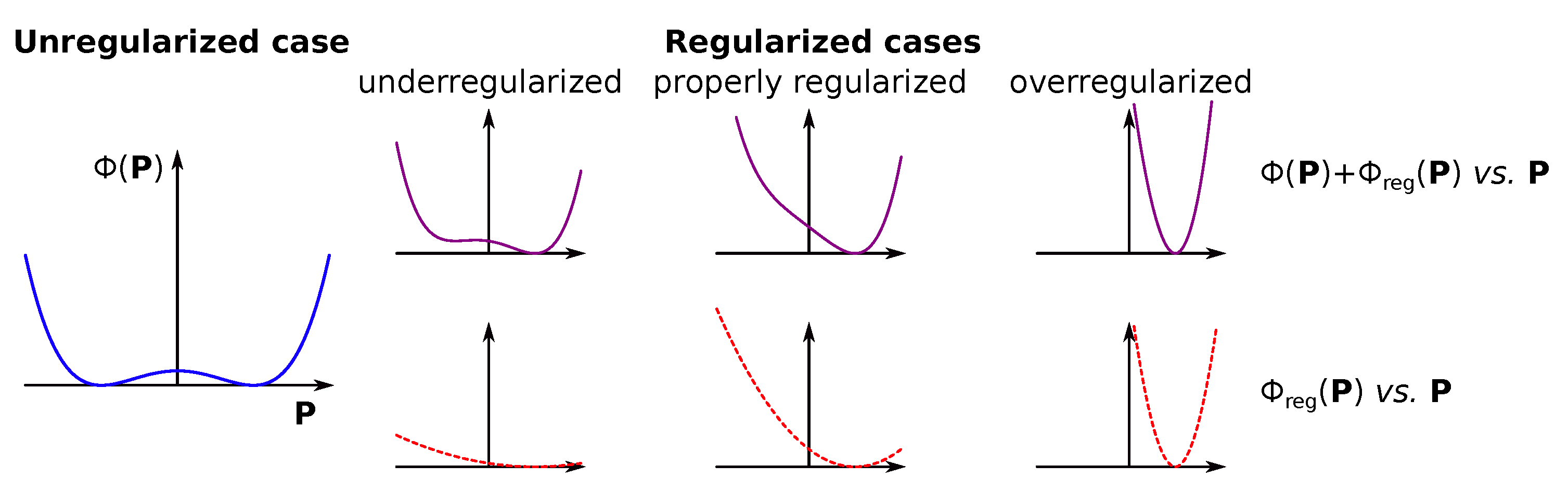
2.3. Regularization of the Least-Squares Inverse Problem

The main method of how to deal with ill-posed inverse problems is the so-called regularization [14,15,16]. The idea of this method is simple: since our experimental data do not provide a single solution to the problem, and we cannot decide which of the solutions is the correct one, we need to get some a priori information to decide on this. In other words, we take some external information on the system and modify the inverse problem to account for this constraining information. We can have pre-known estimate values for some subset of the parameters p P , or even for all of the parameters ( p = P ). Let us denote our known parameters as p reg . To impose soft constraints from these parameters to the LSQ minimization problem (Equation (8)), we can add a penalty function Φ reg ( P ) modifying the inverse problem to:
Φ ( P ) + Φ reg ( P ) min .
The two most common ways to define the regularization term are based on the L 1 or L 2 norms in parameter space. The first one is the so-called L 1 -regularization (or lasso regression) with the penalty function defined as the scaled absolute deviation of the minimized subset of parameters p from the pre-known regularization parameters p reg (i.e., Φ reg ( P ) = λ · | p p reg | ) [23,24]. The second term is the so-called L 2 -regularization (or ridge regression) [15,17]. In this case, the penalty function is defined as a squared deviation of the minimized parameters from the regularization values:
Φ reg ( P ) = λ · p p reg 2 ,
where λ 0 here (and also in the L 1 case) is a regularization parameter. This free parameter determines how strongly the inverse problem in Equation (11) is penalized, i.e., it measures the “softness” of constraints. The effect of the regularization parameter choice is visualized in Figure 2. Let us assume that the LSQ inverse problem has two equivalent solutions. Adding the penalty term skews the results towards one of the two solutions in the regularized inverse problem (Equation (11)). If the regularization parameter is too small, we still may end up with two solutions, and this case is the so-called underregularized inverse problem. If the parameter λ is too large, the penalty term becomes larger than the initial experimental LSQ function ( Φ ( P ) ), which results in the final solution of the inverse problem to be close to the regularization parameters (i.e., p exp p reg ). This case is called overregularized inverse problem. The sweet spot between underregularized and overregularized cases results in the best possible solution. However, this requires a proper choice of the regularization parameter λ . The recipes for the choice of λ are called regularization criteria, and they are widely discussed in the scientific literature [16,25].
An alternative to regularization in the ill-posed nonlinear inverse problems is fixing some of the parameters in P to the pre-computed or pre-known values, e.g., by forcefully setting p = p reg . This reduction of parameter space, in some cases, can make the ill-posed problem to be well-posed. Depending on the field, this approach may have different names [26], but we will call it rigid constraints. This can also be considered an extreme case of regularization, where the regularization parameter is infinite ( λ ). The less widely discussed problem of the regularization and rigid constraints is if the constraints’ values ( p reg ) do not come from the experiment but from theoretical calculations or even as arbitrary assumptions. In this case, the nonexperimental assumptions will strongly influence both the resulting parameters’ values and their uncertainty estimations, as given by Equation (10), making the inverse problem solution only partially experiment-based [20,27]. In the worst case scenarios, the approach of fixing parameters can even lead to nonphysical solutions [28].

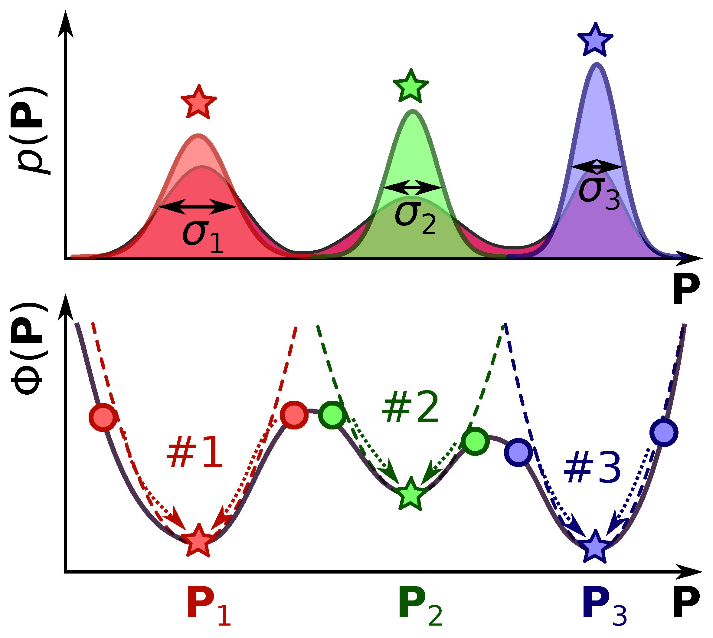
2.4. Monte-Carlo Importance Sampling of the Parameter Space

A more direct approach to obtaining a reliable estimation of the parameters than the LSQ fitting is the Monte-Carlo (MC) sampling of the associated probability distribution, describing the discrepancy between the experimental observations and the model prediction (Equation (5)) [13,14]. In this case, we try to obtain a valid representation of the probability distribution rather than using a local normal distribution (Equation (10)) to approximate the uncertainties of and correlations between the model parameters (see Figure 1).
An effective approach of MC, compared to the naive direct sampling of the whole parameters’ space, is the Metropolis algorithm [29], which is a kind of Markov chain MC [30] method developed for usage in computational physics [31]. In general, the algorithm works as follows [12].
  • We start from the initial set of parameters P ini , which we assign to be the current state of the simulation P current (i.e., we set P current = P ini ). Generally, we can use any set of parameters for the initial guess, but a faster simulation convergence is reached if we provide initial values in the desired solution region, e.g., as the solution of the LSQ fitting problem (Equation (9)).
  • From the current state, we generate a new trial set of parameters P trial , and then we compute the transition probability p ( current trial ) . This value describes a chance of changing our current state P current to a new state P trial (i.e., reassigning P current = P trial ). The probability p ( current trial ) should be related to the probabilities given in Equation (5), and we will discuss it in detail further in the text (see Equation (21)).
  • Then, we draw a random value p ˜ [ 0 ; 1 ) from a uniform distribution between 0 and 1, and compare the p ˜ with p ( current trial ) .
    • If p ˜ p ( current trial ) , then P trial becomes the new state of the system, i.e., we reassign P current = P trial . This state we will call an accepted step.
    • If p ˜ > p ( current trial ) , this means that the transition does not happen (we disregard the P trial ). The new state of the system becomes the same old value P current . We will call this state a declined step.
  • By repeating steps #2 and #3 for a sufficient amount of iterations (N), we generate a trajectory of states P ( n ) , where index n = 1 , 2 , N denotes the state P current at the n-th iteration of the algorithm. Naturally, some sets of parameters will be repeated multiple times throughout the trajectory. Furthermore, this trajectory { P ( n ) } n = 1 N will encode inside the desired distribution given in Equation (5). In practice, the initial part of the trajectory (e.g., first 10% of steps) is disregarded as an equilibration phase. The acceptance ratio refers to the accepted steps in algorithm step #3 ( N acc ) to the total number of steps ( N tot = N acc + N rej , where N rej is the number of rejected steps). A general requirement for the simulation to be reasonably good is that this ratio should not be too big or too small. A simple rule of thumb can be that the acceptance rate R acc = 100 % · N acc / N tot should be in the range 10 % R acc 50 % .
  • From the obtained trajectory { P ( n ) } n = 1 N , we can compute all the required parameters. For instance, the mean value of parameter P k (from the set of parameters P ) can be computed as:
    P k = 1 N n = 1 N P k ( n ) ,
    where P k ( n ) is the value of P k in the parameter set P ( n ) . Similarly, we can compute the standard deviation σ k of parameter P k from the mean value as:
    σ k 2 = P k 2 P k 2 = 1 N n = 1 N P k ( n ) 2 1 N n = 1 N P k ( n ) 2 .
    The covariance between the parameters P k and P l will be given similarly, as:
    cov ( P k , P l ) = P k P l P k · P l =   = 1 N n = 1 N P k ( n ) · P l ( n ) 1 N n = 1 N P k ( n ) · 1 N n = 1 N P l ( n ) .
    From standard deviations (Equation (14)) and covariances (Equation (15)), we can also calculate the Pearson’s correlation coefficients between parameters P k and P l as:
    ρ ( P k , P l ) = cov ( P k , P l ) σ k · σ l .
Using this algorithm, we can effectively sample the possible solutions and provide a more general estimation of parameter values and their uncertainties.
The only aspect missing in the algorithm is the actual expression for the transition probability p ( current trial ) . For that, we need to consider a condition of the detailed balance. In order for Equations (13)–(15) to work, the probability from Equation (5) should be inherently contained within the trajectory { P ( n ) } n = 1 N of N steps. It means that for a given state P , it should be contained within the trajectory N ( P ) times, which should be given through the probability of this state:
p ( P ) = N · exp ( Φ ( P ) ) N ( P ) N ,
according to Equation (5). Note that, in general, we do not know the normalization factor N . Since we have a random procedure, if we take two possible parameter sets, say P and P , and consider that we have a possibility to go from one to another, and vice versa, these jumps between P and P should not spoil the inherent probability in the trajectory (Equation (17)). This can be fulfilled if we balance the number of jumps from P to P , and back, to be equal. The number of transitions from P to P ( N ( P P ) ) is simply the total number of points with state P times the transition probability p ( P P ) , that is:
N ( P P ) = N ( P ) · p ( P P ) = N · N · exp ( Φ ( P ) ) · p ( P P ) .
A similar expression can be derived for the number of transitions from P to P :
N ( P P ) = N ( P ) · p ( P P ) = N · N · exp ( Φ ( P ) ) · p ( P P ) .
By setting N ( P P ) = N ( P P ) , we can assure that the MC procedure will not change the proper probability distribution. This condition is called the detailed balance. If the MC procedure follows this principle, it produces the desired trajectory with the probability encoded inside the distribution of points within the trajectory. Substitution of Equations (18) and (19) to the detailed balance results in:
exp ( Φ ( P ) ) · p ( P P ) = exp ( Φ ( P ) ) · p ( P P ) .
Any transition probability p ( P P ) fulfilling the detailed balance given in Equation (20) is suitable for the MC simulations [12]. The simplest choice for the transition probability is the following [29]:
p ( P P ) = S · min exp Φ ( P ) Φ ( P ) , 1 =     = S · 1 , if Φ ( P ) Φ ( P ) 0 , exp Φ ( P ) Φ ( P ) , if Φ ( P ) Φ ( P ) < 0 .
Let us comment on Equation (21). The parameter S > 0 is just an arbitrary scaling factor that could be used to change the acceptance rate R acc in the MC simulation. We will consider it for now to be S = 1 . If Φ ( P ) > Φ ( P ) , i.e., the LSQ function (Equation (6)) for the new set of parameters P is smaller than for the old set P , we get exp ( Φ ( P ) Φ ( P ) ) > 1 , which will give us the probability p ( P P ) = 1 . In other words, if a trial set of parameters is better than the previous one, we definitely accept the new parameters. If the new set of parameters is worse than the old one ( Φ ( P ) < Φ ( P ) ), the probability of accepting the new configuration will be exp Φ ( P ) Φ ( P ) < 1 , and the worse the new parameters are compared to the old ones, the less probable their acceptance will be.
As was discussed above, the optimal acceptance rate of the MC sampling ( R acc ) should be in the range of 10 % R acc 50 % . This rate is being controlled by two factors: (1) generation procedure of the trial parameters P trial and (2) transition probability (Equation (21)). Therefore, we have two ways of controlling the R acc in the MC sampling procedure. First, we can adjust the trial parameters generation, e.g., reducing/increasing the size of the steps from the current configuration to increase/decrease R acc , respectively. Secondly, we can decrease/increase the scaling factor S value in Equation (21) to decrease/increase R acc , respectively. However, the second approach is less delicate than the first one.

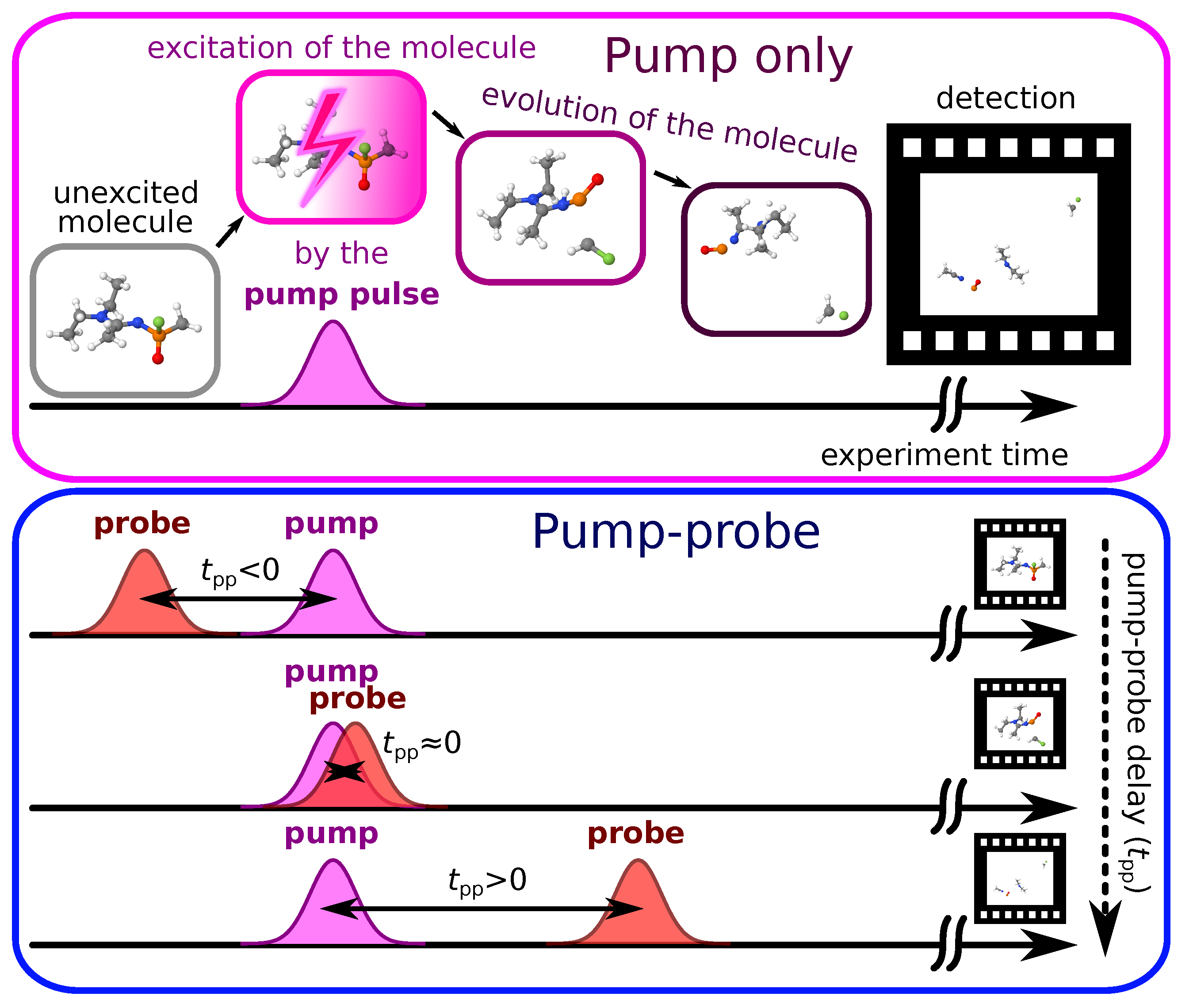
3. Fitting Model of Pump–Probe Spectroscopy

3.1. General Considerations

As explained in the previous Section 2, we require a model of the experiment to solve both the direct (Equation (1)) and inverse problems (Equation (3)). The pump–probe experiment can be imagined as shown in Figure 3. It consists of multiple experiments that only differ in the delay time between pump and probe pulses (pump–probe delay, t pp ). With the pump pulse, we initiate the reactions, and with the probe pulse, we change the stable and metastable intermediate products of interaction into the observable results [1,2,4,18]. In all the further discussion here, we will use a convention shown in Figure 3, that is:
  • If both the pump and the probe pulses act on the molecule simultaneously, then t pp = 0 (this temporal overlap of the pump and probe pulses is also called t 0 );
  • If the probe pulse interacts with the molecule before the pump pulse, then t pp < 0 ;
  • If the probe pulse interacts with the molecule after the pump pulse, then t pp > 0 .
Figure 3. A schematic illustration of the idea of the pump–probe spectroscopic experiment. The (top) part of the image illustrates what happens in time in the experiment if only the pump pulse is given. First, we introduce the molecular system in the apparatus, then we excite our molecular system with the pump pulse, and then the photochemically induced changes happen in the system on various timescales. In the end, we collect the signal produced by the molecular system at an infinitely distant time. In the pump–probe case (bottom), we perform multiple experiments of such sort, but introducing the second pulse, the probe, with some delay with respect to the pump pulse (pump–probe delay, t pp ). The changes in the observed signal as a function of t pp form the pump–probe signal, potentially carrying information of the intermediate species.
Photochem 04 00005 g003
We can model all the photochemical processes happening in the pump–probe experiment with chemical kinetic equations, where we define the cross-sections of various processes, such as the interaction with light, branching ratios, and rate constants for various relaxation processes, and then integrate the resulting set of first-order differential equations in time to get our observables [32,33]. In the cases with quantum beating between different states, we also can switch from simple chemical kinetics equations to the Maxwell–Bloch equations formulated in terms of the density matrix of the molecular system [4,34]. The general shape of the equations is very similar, but in Maxwell–Bloch equations, the evolution of the off-diagonal density matrix elements is added. Both explicit dynamics approaches successfully disentangled complex dynamics in various pump–probe experiments [5,10,35,36].
However, modeling the rate dynamics explicitly is rather complicated and time-consuming. First, the cost of solving the differential equations is higher than many other numerical problems. This can be a significant drawback, especially for inverse problems where we are trying to evaluate multiple parameters. In the case of standard LSQ minimization (see Section 2.2), where we need a lot of calculations with various parameters at each minimization iteration, a slow direct model can drastically limit the number of varying parameters. It is even worse in the case of MC sampling (see Section 2.4), where we need as many steps as possible to get the best possible sampling of the parameter space. Second, solving the differential equations can be nontrivial. For instance, the rates of the intramolecular relaxation processes can be on the order of a few tens of femtoseconds, while the isomerization and formation of the fragments that are observed with the mass spectrometer can take multi-picosecond timescales [10]. Such a large variety of timescales requires a careful choice of integration techniques, especially for large pump–probe delays. Another complication for explicit kinetic modeling is the existence of parasitic processes, in which the molecular system’s dynamics is initiated not by the pump but by the probe pulse and then probed by the pump pulse [6,37]. Such processes require additional integration of the kinetic equations in the “backward” time direction.
Therefore, in the cases of many observables and parameters, the model-based approaches that describe observables in terms of given functions are more advantageous for solving the inverse problem [38]. Here, we will, thus, only consider such a model approach. We will generally follow the classical work of Pedersen and Zewail [18], but try to show these well-known results from a simpler perspective and also extend the classical equations to the case of coherent oscillations in pump–probe observables [8,10].

3.2. Delta-Shaped Pump–Probe Model

3.2.1. Assumptions of the Model

First, we will consider an ideal case of the pump–probe experiment in which pump and probe pulses have zero temporal width. Both pump and probe pulses instantly convert the molecular system into something else upon interaction. We will also consider the pump–probe delay t pp to be exactly known without any imperfections. In this case, we can try to devise what the results of our pump–probe experiment will be that we will observe. We will use photochemical reaction schemes and chemical kinetics equations to obtain numerical expressions for the pump–probe delay-dependent signals [39,40]. In all cases, we will assume that all the chemical reactions induced are monomolecular first-order reactions. Such an assumption is certainly true for all gas-phase experiments and usually also holds for ultrafast pump–probe processes in the medium [33,38].

3.2.2. Step Function Dynamics

First, let us consider this simple pump–probe reaction scheme:
M + pump A A + probe B ,
where we have our initial molecule (M), which interacts with photons of the pump pulse to produce the initially unexistent stable chemical A. Then, this newly formed product A can interact with the photons of the probe pulse to produce compound B. Such a pump–probe reaction scheme is quite ubiquitous in real-life experiments. For instance, in the case of polycyclic aromatic hydrocarbons (PAHs), upon interaction with high-energy extreme ultraviolet (XUV) photons, stable mono- or dications can be formed, which then can fragment into smaller ions upon interaction with the probe pulse (see, e.g., [6,7]).
Let us now discuss what would be observed in the reaction scheme (22) for species A and B, and the number of unabsorbed probe photons. At t pp < 0 (i.e., when the probe acts before the pump), we would see a constant amount of the product A, no molecules B, and a fully unabsorbed probe pulse. Then, for t pp > 0 , we would also see a constant amount of molecules A, but smaller than it was for t pp < 0 , since now some of the A would be lost by the second reaction in the reaction scheme (Equation (22)). A similar behavior would be observed for the probe pulse: its intensity would be constant but depleted since some of the probe photons would be lost in interaction with A. For B, we would see some constant amount of signal. At t pp = 0 , we would have an instant switch of behavior for all of the observables. Therefore, we can formalize the signal observed for all species (A, B) and the probe pulse intensity as follows:
f ( t pp ) = f 0 + 0 , t pp < 0 f 1 , t pp 0 = f 0 + f 1 · θ ( t pp ) ,
where f 0 and f 1 are constants, f 0 indicates the initial/final amount of the given species, and f 1 characterizes the cross-section for the interaction between A and probe photons. Function θ ( t ) is the Heaviside step function, defined as:
θ ( t ) = 0 , t < 0 1 , t 0 .
For the amount of A and intensity of the probe pulse, we will get f 0 > 0 , f 1 < 0 , and for B, it will be f 0 = 0 and f 1 > 0 . Although, theoretically, the magnitude of f 1 for A and B in the reaction scheme (22) should be equal, in practice, the signal magnitude can be different due to the various factors, such as parasitic reactions, different detector efficiency, or even differences in the integration windows for the signal (e.g., in the mass spectra). Nevertheless, the general shape of the signals will be similar.

3.2.3. Instant Dynamics

Another simplistic pump–probe behavior is the instant dynamics, in which the observable product A can be produced from the initial molecule M only if pump and probe pulses simultaneously act on M. This type of photochemical reaction can be formally written as:
M + pump + probe A .
Processes of this type can also be found in real-life experiments. For instance, the dynamics of the formation of photoelectron side bands follows this kinetic scheme (see Refs. [6,41]). Such instant dynamics processes are useful in ultrafast experiments with X-ray free electron lasers (FELs) because they allow for precise determination of the temporal overlap between pump and probe pulses ( t 0 or t pp = 0 ).
Since both the pump and probe pulses in our model have zero duration, the only possible way to formally write the yield of A as a function of pump–probe delay t pp is as follows:
f ( t pp ) = f 0 · δ ( t pp ) ,
where f 0 is a constant, characterizing the cross-section of reaction (25), and δ ( t ) is the Dirac delta function (i.e., δ ( 0 ) and δ ( t ) = 0 for t 0 ).

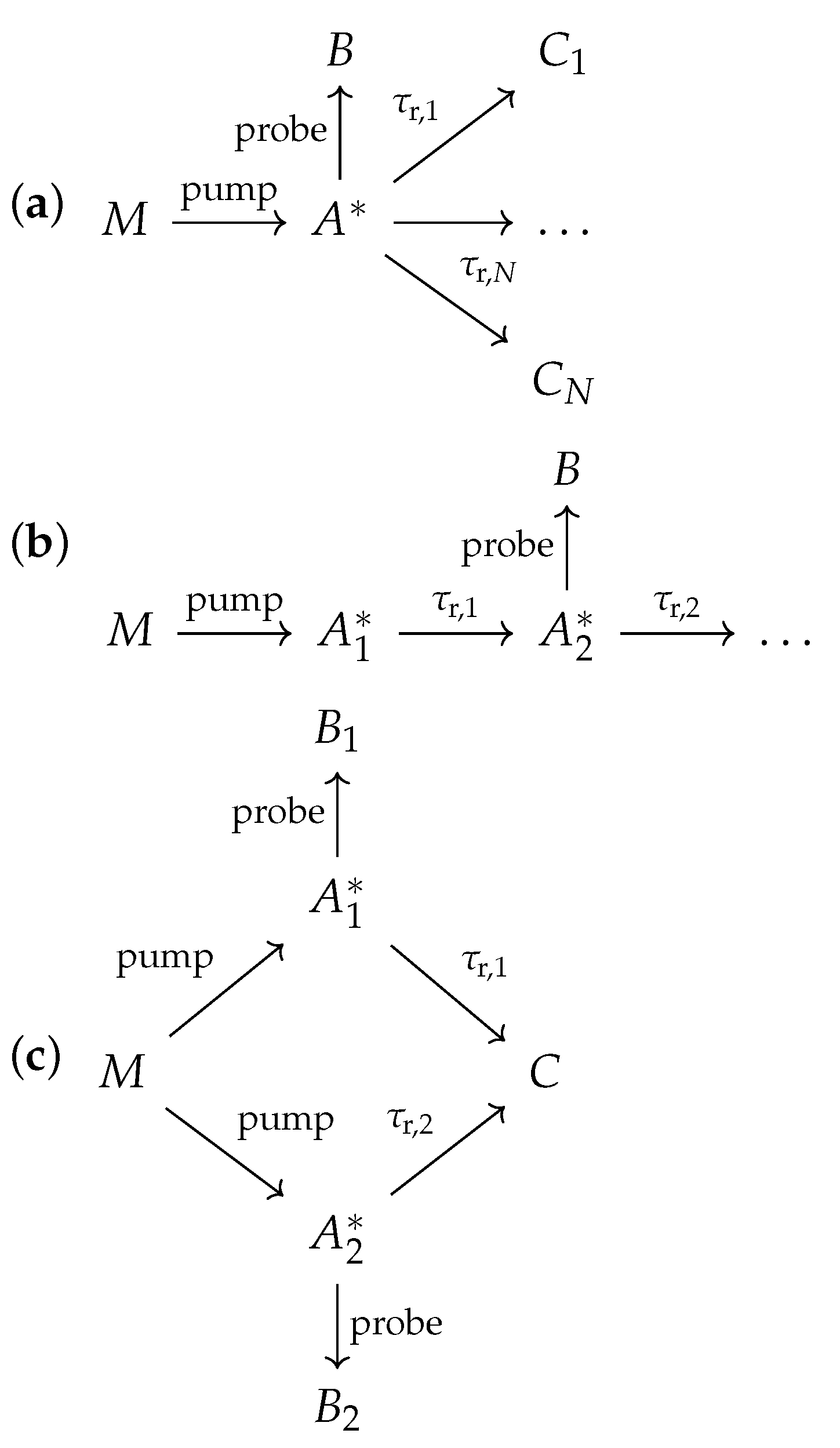
3.2.4. Transient Pump–Probe Signatures of Metastable Species

The pump–probe studies’ desirable products are the metastable species’ signatures. The basic model of their dynamic behavior can be described with the following reaction scheme:
M + pump A * A * k r C A * + probe B ,
where we again denote the initial molecule as M and the final observable species as C and B, but now we have a metastable species A * that spontaneously converts into C with a first-order reaction rate k r . We assume this decay rate to be too fast for A * itself to be detectable with the experimental setup. However, while we still have A * present in the system, we can convert it into the observable species B.
For the reaction scheme (27), we now need to consider the evolution of A * in real experimental time, which we will denote as t 0 . At t = 0 , we obtain [ A * ] 0 as the initial concentration of A * , which is created by the pump pulse. Then, at t > 0 , A * decays into C with the rate constant k r . The rate equation for the concentration of A * molecules ( [ A * ] = [ A * ] ( t ) ) from the scheme (27) is written as [39,40]:
d [ A * ] d t = k r [ A * ] ,
which results in the following solution (see Appendix A.1):
[ A * ] ( t ) = [ A * ] 0 · exp ( k r t ) = [ A * ] 0 · 2 t τ 1 / 2 = [ A * ] 0 · exp ( t / τ r ) ,
where we provide the three most common ways to write the result, using the rate constant k r , half-life time τ 1 / 2 = ln ( 2 ) / k r , which gives the time at which the concentration [ A * ] becomes half of which it was initially, and decay time:
τ r = 1 k r = τ 1 / 2 ln ( 2 ) ,
which indicates the time at which the concentration [ A * ] becomes e 2.72 times smaller than initially. In further discussions, we will only use the decay time τ r .
Knowing the decay of A * , we can also find the evolution of C in the experimental real time. The rate equation for the concentration of C ( [ C ] ) from the reaction scheme (27) is [39,40]:
d [ C ] d t = + k r [ A * ] .
At the initial time, we do not have any C, and thus, [ C ] ( 0 ) = 0 . Integration of Equation (31) with [ A * ] given by Equation (29) (see Appendix A.1) is as follows:
[ C ] ( t ) = [ A * ] 0 · 1 exp t / τ r .
Knowing the dynamics of A * and C (Equations (29) and (32)), we can describe how the change in yields of C and B would behave as a function of the pump–probe delay t pp . At t pp < 0 , A * is produced after the probe pulse has already passed the system. Thus, the total amount of B is zero. As for C, we assume that the time of detection by the experimental instrument t instr is infinite compared to the internal dynamics time τ r ( t instr τ r ). This means that the amount of registered C molecules at t instr from Equation (32) is [ C ] ( t instr ) [ A * ] 0 , i.e., all A * intermediate is fully converted into C before the detection. At t pp 0 , the probe pulse will instantly convert part of A * into B according to the last equation in the reaction scheme (27). If we denote the conversion efficiency of the probe pulse interaction as 0 p 1 , then the resulting concentration of B is [ B ] = p · [ A * ] ( t pp ) = p · [ A * ] 0 · exp ( t pp / τ r ) . The amount of C at t pp 0 , that we will register at t instr , will be the difference between the full conversion result and the part of A * lost upon conversion into B by the probe, i.e., [ C ] ( t instr , t pp ) = [ A * ] 0 [ A * ] ( t pp ) = [ A * ] 0 · ( 1 p · exp ( t pp / τ r ) ) .
We can combine the described yields of B and C as functions of pump–probe delay t pp using the Heaviside function (Equation (24)) as:
[ B ] ( t pp ) = [ A * ] 0 · p · θ ( t pp ) exp ( t pp / τ r ) , [ C ] ( t pp ) = [ A * ] 0 · 1 p · θ ( t pp ) exp ( t pp / τ r ) .
The yield of C resembles the formation kinetics of C in real experimental time (Equation (32)), while for B it resembles the real experimental time dynamics of the unstable intermediate A * (Equation (29)). Nevertheless, we can summarize both of these dependencies with a general expression of the form:
f ( t pp ) = f 0 + f 1 · θ ( t pp ) exp ( t pp / τ r ) ,
where f 0 and f 1 are again constants proportional to the cross-section of the pump/probe photons interacting with the molecular species.
Equation (34) has an intriguing similarity with Equation (23), describing the pump–probe dynamics according to reaction scheme (22). This similarity is not a coincidence, since if A * is stable (i.e., k r = 0 , or τ r ), the reaction scheme (27) collapses into the reaction scheme (22). Equation (34) will be transferred into Equation (23), if | t pp | τ r , since in this case exp ( t pp / τ r ) 1 . Similarly, the reaction scheme transforms into reaction scheme (25) if A * is too unstable (i.e., k r , or τ r 0 ). In this case, the decay exponent becomes localized near t pp = 0 , which can be approximated by Equation (26).

3.2.5. Coherent Oscillations without Decay

We worked with standard chemical kinetics equations in the previous model (Equation (27)). However, if we want to discuss periodic oscillation features that are being observed in some pump–probe experiments [8,10,42], such semiclassical description turns out to be insufficient, and a quantum-mechanical model has to be used. Here, we will provide the simplest model for such behavior based on a two-level quantum system. First, we will discuss a basic model without the decay dynamics, and then we will modify our model to include the decay effects [43,44].
Let us imagine that our molecular system is described with a Hamiltonian H ^ , which has eigenstates | 0 and | 1 , that are solutions to the stationary Schrödinger equation H ^ | k = E k | k ( k = 0 , 1 ). These states will be considered to be orthonormal, i.e., k | l = δ k l for k , l = 0 , 1 . We will take the energy E 0 of the ground state | 0 as a reference, i.e., as zero ( E 0 = 0 ). The energy of the excited state | 1 will be denoted as E 1 = ω , where is the reduced Planck constant and ω is the angular frequency of the photon that provides excitation from the ground to the excited state ( | 0 | 1 ). Note that ω is related to the normal frequency ν as ω = 2 π ν . Now, we will consider the evolution of this system in real-time t with explicit inclusion of the effects of the pump and probe pulses.
Suppose now that the system was initially in the ground state, i.e., before the pump pulse acted on the system, the wavefunction of the system was as follows:
| ψ ini = | 0 .
After instant action, the pump pulse at real-time t = 0 has created a superposition state, transferring some population to the excited state. The new state of the system right after the pump pulse at t = 0 is described as:
| ψ ( 0 ) = c 0 | 0 + c 1 exp ( i φ ) | 1 ,
where c 0 and c 1 are the coefficients, showing the amount of the system in the ground and excited states as | c 0 | 2 and | c 1 | 2 , respectively, with a condition of | c 0 | 2 + | c 1 | 2 = 1 , and φ is the phase of the excited state related to the ground state, which is imposed, e.g., by the phase of the excitation pump pulse [45,46].
To propagate the dynamics of the state after interaction with the pump pulse (Equation (36)), let us switch to the density matrix formalism. The density matrix ρ ^ for our two-level system in the basis of states | 0 and | 1 is written as:
ρ ^ = ρ 00 | 0 0 | + ρ 01 | 0 1 | + ρ 10 | 1 0 | + ρ 11 | 1 1 | ,
where the coefficients ρ k l ( k , l = 0 , 1 ) describe the state of the system. This form can be rewritten in the form of an actual matrix by placing the coefficients accordingly as:
ϱ = ρ 00 ρ 01 ρ 10 ρ 11 .
The elements of this matrix should fulfill two requirements. First, the trace of this matrix should be equal to one ( tr ( ϱ ) = ρ 00 + ρ 11 = 1 ). Second, the matrix ϱ should be Hermitian, which means ρ 01 = ρ 10 * .
The density matrix ρ ^ for our system at time t = 0 can be obtained from the initial state | ψ ( 0 ) (Equation (36)) as:
ρ ^ ( 0 ) = | ψ ( 0 ) ψ ( 0 ) | = = | c 0 | 2 ρ 00 ( 0 ) | 0 0 | + c 0 c 1 * exp ( + i φ ) ρ 01 ( 0 ) | 0 1 | + c 0 * c 1 exp ( i φ ) ρ 10 ( 0 ) | 1 0 | + | c 1 | 2 ρ 11 ( 0 ) | 1 1 | .
Let us consider c 0 and c 1 as real values, concealing all the complex behavior into the phase φ . We can also denote c 1 2 = p and c 0 2 = ( 1 p ) , where 0 p 1 is the efficiency of the pump pulse excitation | 0 | 1 . In this case, the initial parameters of the matrix from Equation (38) will be:
ρ 00 ( 0 ) = 1 p , ρ 01 ( 0 ) = p · ( 1 p ) exp ( + i φ ) , ρ 10 ( 0 ) = p · ( 1 p ) exp ( i φ ) , ρ 11 ( 0 ) = p .
As can be seen, the diagonal elements ( ρ 00 and ρ 11 ) encode the population in a given state, and the off-diagonal elements ( ρ 01 and ρ 10 ) encode coherence between the levels.
The density matrix ϱ evolves according to the von Neumann equation [44]:
i d ϱ d t = [ H , ϱ ] ,
where [ a , b ] = a b b a is the commutator and H is the Hamiltonian matrix composed of the elements k | H ^ | l , which in our basis of orthonormal eigenstates looks as follows:
H = 0 | H ^ | 0 0 | H ^ | 1 1 | H ^ | 0 1 | H ^ | 1 = 0 0 0 ω .
Substituting the density matrix (Equation (38)) and the Hamiltonian matrix (Equation (42)) into the von Neumann equation (Equation (41)), we find the following equations for the evolution of each of the density matrix elements (details in Appendix A.2):
d ρ 00 d t = 0 , d ρ 11 d t = 0 , d ρ 01 d t = + i ω ρ 01 , d ρ 10 d t = i ω ρ 10 .
Solutions of these equations (see in Appendix A.2) with initial conditions given in Equation (40) are:
ρ 00 ( t ) = 1 p , ρ 11 ( t ) = p , ρ 01 ( t ) = p · ( 1 p ) · exp ( + i φ + i ω t ) , ρ 10 ( t ) = p · ( 1 p ) · exp ( i φ i ω t ) .
These results describe the state of the free-evolving molecular system at experiment times t 0 after the pump excitation. Based on this solution, we want to numerically quantify the observables that we will get upon interaction with the probe pulse.
Let us consider that observables O in quantum mechanics are given in the form of operators O ^ . Therefore, we can assume that the result of measurement by the probe will be given by an observable operator O ^ . In the case of our two-level system, we can represent this operator in the matrix form similar to the Hamiltonian (Equation (42)):
O = O 00 O 01 O 10 O 11 ,
where the matrix elements are the following integrals:
O k l = k | O ^ | l , k , l = 0 , 1 .
We will assume that all these integrals are real, and thus, O 01 = O 10 .
The mean result of the observable measurement O of the system described by the density matrix ϱ (Equation (38)) is given as a trace of the product between matrices O and ϱ :
O = tr ( O ϱ ) = O 00 ρ 00 + O 01 ρ 10 + O 10 ρ 01 + O 11 ρ 11 .
By measuring the state described by the density matrix with elements from Equation (44) in real time equal to the pump–probe delay ( t = t pp ), and taking into account that O 01 = O 10 as well as Euler’s formula ( exp ( i x ) = cos ( x ) + i sin ( x ) ), we obtain the pump–probe signal at t pp 0 to be:
O ( t pp ) = O 00 · ρ 00 ( t pp ) ( 1 p ) + O 01 · ρ 10 ( t pp ) p · ( 1 p ) · exp ( i φ i ω t pp ) + + O 10 O 01 · ρ 01 ( t pp ) p · ( 1 p ) · exp ( + i φ + i ω t pp ) + O 11 · ρ 11 ( t pp ) p = = O 00 · ( 1 p ) + O 11 · p f 1 + 2 O 01 p · ( 1 p ) f 2 · cos ( ω t pp + φ ) = = f 1 + f 2 · cos ( ω t pp + φ )
At pump–probe delay times t pp < 0 (i.e., when the probe acts before the pump), the probe pulse will observe the initial state of the system (Equation (35)), which can be represented (similarly to that in Equation (39)) by a density matrix:
ϱ ini = 1 0 0 0 ,
which upon substitution to Equation (47) will provide us with probe results at delays t pp < 0 :
O ( t pp ) = tr ( O ϱ ini ) = O 00 = f 0 .
Now, we can merge the results of the pump–probe experiment result ( f ( t pp ) = O ( t pp ) ) for our two-level molecular system for pump–probe delays t pp < 0 (Equation (50)) and t pp 0 (Equation (48)) to obtain:
f ( t pp ) = f 0 + f 1 · θ ( t pp ) + f 2 · θ ( t pp ) · cos ( ω t + φ ) .
In this equation, the coefficients f k ( k = 0 , 1 , 2 ) are again proportional to the cross-sections of pump/probe interaction with the molecules, the oscillation frequency ω encodes the energy difference between two coherent states | 0 and | 1 through the Planck relation E 1 E 0 = ω , and initial phase of the oscillation φ is an imprint of the pump pulse’s phase. In the incoherent regime of the system’s excitation, the oscillating term disappears, and Equation (51) converts into the classical Equation (23) (see Appendix A.3 for details). Such correspondence between quantum and classical cases is not a coincidence: both cases refer to the same reaction scheme (22), wherein the quantum case, M is | 0 , A is | 1 , and instead of providing a concrete yield of observable, we use a more generic treatment of the probe with the operator O ^ .

3.2.6. Coherent Oscillations with Decay

Now, we will discuss the dynamics of the two-level system in which the excited state can decay back into the ground state after the excitation. The derivation procedure will be the same as in the previous Section 3.2.5. Therefore, we only highlight the changes that will lead to a new result.
We start with the same system described generally by a 2 × 2 density matrix (Equation (38)). Before the pump, the molecular system is described by a wavefunction from Equation (35) and right after the pumping, by a wavefunction from Equation (36). Equivalently, they are given by a density matrix from Equations (40) and (49), respectively. Therefore, we again need to propagate the pumped state.
To do the propagation, we will replace the von Neumann Equation (41) with its modified version, the Lindblad equation, which considers the decay between states. In our case, we can represent it as follows [44,47]:
i d ϱ d t = [ H , ϱ ] + i γ σ ϱ σ + 1 2 { σ + σ , ϱ } ,
where the first part of the equation is the same as in Equation (41), and in the added decay term, γ is the rate of the decay, { a , b } = a b + b a is the anticommutator, and the σ ± matrices are the excitation/deexcitation operators of the following form [44,47]:
σ + = 0 0 1 0 and σ = 0 1 0 0 .
We can rewrite Equation (52) for our system (similarly to Equation (43)) as follows (see Appendix A.4):
d ρ 00 d t = + γ ρ 11 , d ρ 01 d t = + i ω ρ 01 1 2 γ ρ 01 , d ρ 10 d t = i ω ρ 10 1 2 γ ρ 10 . d ρ 11 d t = γ ρ 11 .
Solving these equations with initial conditions given in Equation (40) results in the following results:
ρ 00 ( t ) = 1 p · exp ( γ t ) , ρ 11 ( t ) = p · exp ( γ t ) , ρ 01 ( t ) = p · ( 1 p ) · exp ( + i φ + i ω t ) · exp γ t 2 , ρ 10 ( t ) = p · ( 1 p ) · exp ( i φ i ω t ) · exp γ t 2 ,
where we obtain decay dynamics with the rate k r = γ . Therefore, to be in line with the previous notation, we will replace γ with the decay time τ r according to Equation (30).
Now, substituting the density matrix elements from Equation (55) into Equation (47), describing the observable at t pp 0 , we obtain a following analog of Equation (48):
O ( t pp ) = O 00 f 1 + p · O 00 + O 11 f 2 · exp t pp τ r + + 2 O 01 p · ( 1 p ) f 3 · cos ( ω t pp + φ ) · exp t pp 2 τ r = = f 1 + f 2 · exp t pp τ r + f 3 · cos ( ω t pp + φ ) · exp t pp 2 τ r .
The behavior of this system at delays t pp < 0 stays the same as before (Equation (50)). By combining Equations (50) and (56), we get the coherent decay dynamics observables in the pump–probe domain in the following form:
f ( t pp ) = f 0 + f 1 · θ ( t pp ) + f 2 · θ ( t pp ) · exp t pp τ r + + f 3 · θ ( t pp ) · cos ( ω t + φ ) · exp t pp 2 τ r .
This equation closely reminds us of Equation (51), which can be obtained again in the limit of τ r ( γ = 0 ). At the same time, coherent oscillation dynamics resemble a pump–probe yield from Equation (34), which is restored in the classical limit (see Appendix A.3). This is again no coincidence since the currently discussed pump–probe system is a modification of the reaction scheme (27) with M being | 0 and A * being | 1 . The difference between our two-level quantum model and rate scheme (27) is again in a generic view on the probing, but also in the decay of A * back to M ( A * M instead of A * C in scheme (27)). We could also include the third state emulating C. This would require extending the two-level system to three levels. However, in the three-level system, the pump–probe observables will still be described with Equation (57).

3.2.7. More Complicated Dynamics Models

Now, let us take a look at more complicated reaction models for the pump–probe dynamics than we have looked at before (Equations (22), (25) and (27)). The three extensions can be seen in Figure 4, where scheme (a) shows a possibility of branching reactions when a single metastable intermediate A * can result in multiple products, scheme (b) demonstrates the possibility of having multiple interconverting metastable intermediates, and scheme (c) shows how multiple pathways can produce the same product. However, if we evaluate the observables from these schemes in the pump–probe domain, we see that all of them can be described with the following expression (see Appendix A.5, Appendix A.6 and Appendix A.7):
f ( t pp ) = f 0 + f 1 · θ ( t pp ) + f 2 · θ ( t pp ) · exp t τ ˜ 2 + f 3 · θ ( t pp ) · exp t τ ˜ 3 ,
where τ ˜ i ( i = 2 , 3 ) are effective rate constants computed from original elementary rate constants τ r , j and f i ( 0 i 3 ) are effective parameters, dependent on the pump/probe interaction cross-sections and on the reaction scheme.
The apparent simplicity of Equation (58) can be considered a lucky coincidence for pre-designed schemes, but it is not. In fact, it can be explicitly shown (see Appendix A.8) that if the reaction scheme for the pump-induced dynamics consists only of first-order reactions (i.e., of the type A C 1 + C 2 + ) and the probing dynamics is given only as instant interconversion between species (i.e., of the type A + pump B ), then the pump–probe yield for any of the products is given as:
f ( t pp ) = f 0 · 1 + f 1 · θ ( t pp ) + i 2 f i · θ ( t pp ) · exp t τ r , i ,
where τ r , i ( i = 2 , ) are some effective rate constants composed of the rate constants for individual reactions and the sum over i = 2 , covers all the effective decay pathways.
We can generalize Equation (59) in the following form:
f ( t pp ) = i = 1 N f i · b i ( t pp ) ,
which is just a linear combination of N linearly independent basis functions b i ( t pp ) with coefficients f i . Equation (59) has the following three types of basis functions:
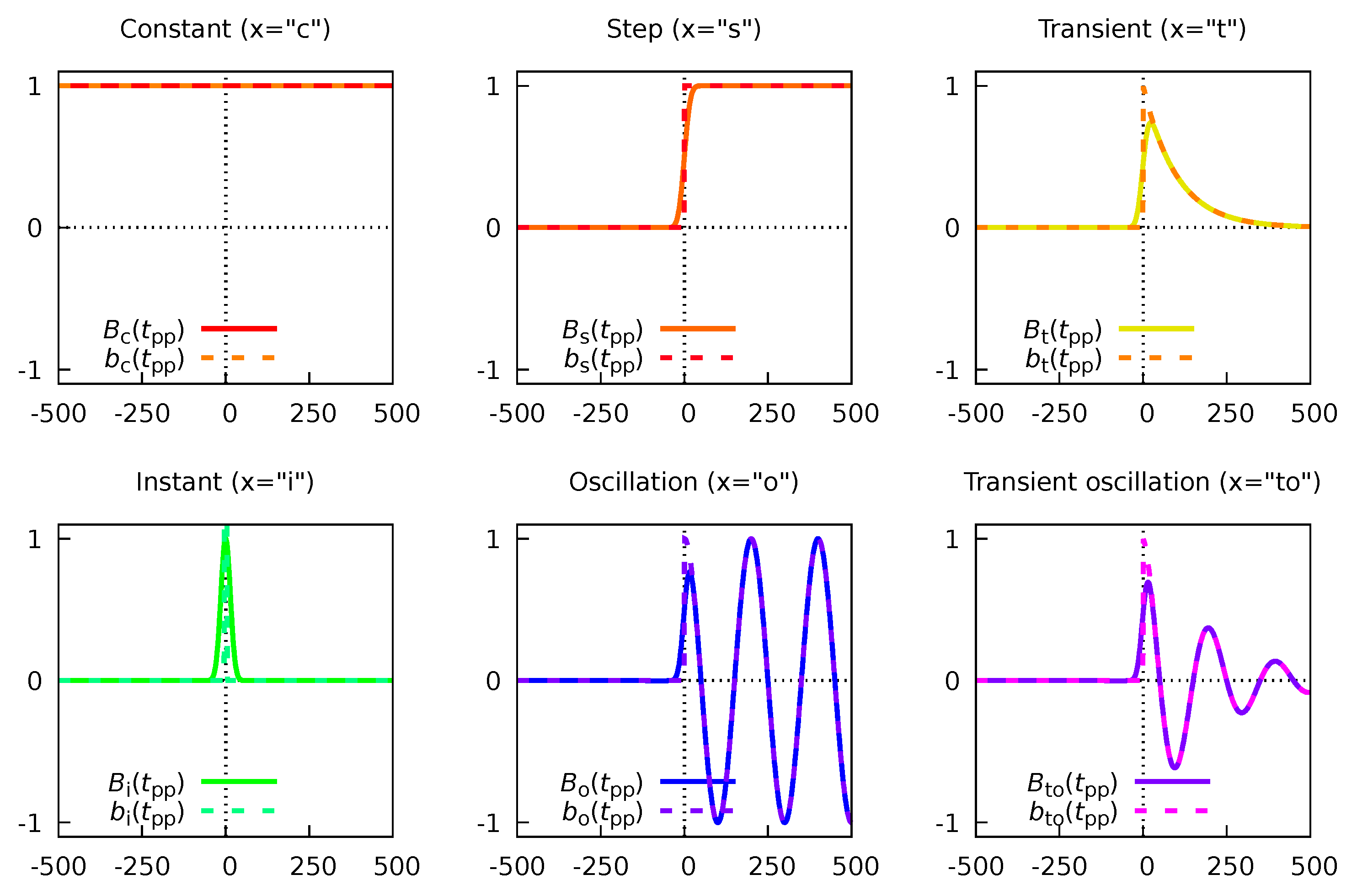
  • The first type is simply the constant (“c”) defined as:
    b c ( t pp ) = 1 .
    This function (with coefficient f 0 in Equation (59)) has no parameters and describes the background of the pump–probe experiment.
  • The second type is the step or “switch” function (“s”):
    b s ( t pp ) = θ ( t pp ) .
    This basis function (with coefficient f 1 in Equation (59)) describes the switching of the background between t pp < 0 and t pp 0 regimes.
  • The third type is the transient (“t”) function:
    b t ( t pp ) = θ ( t pp ) · exp t τ r .
    This type of basis function (with coefficients f i , i 2 in Equation (59)) describes the pump-induced decay dynamics, and it depends on a parameter τ r , which is an effective decay time.
We can augment the three types of basis functions (Equations (61)–(63)) with three additional functions.
  • First, it is the instant (“i”) dynamics (Equation (25)) found in Equation (26):
    b i ( t pp ) = δ ( t pp ) .
    This type of dynamics describes unresolvably fast relaxation dynamics.
  • The second additional function, describing nondecaying coherent oscillation (“o”), can be taken from Equation (51):
    b o ( t pp ) = θ ( t pp ) · cos ( ω t + φ ) .
    This basis function has two parameters: the oscillation frequency ω and the initial phase φ .
  • The last additional function, describing a transient coherent oscillation (“to”), can be taken from Equation (57):
    b to ( t pp ) = θ ( t pp ) · exp t 2 τ r · cos ( ω t + φ ) .
    This basis function has three parameters: the oscillation frequency ω , the initial phase φ , and the decay time τ r .
Using these six basis functions, b c , b s , b t , b i , b o , and b to given with Equations (61)–(66), we can describe any pump–probe observable using expression (60). In the previous discussion, we assumed that the pump pulse only initialized the dynamics and that the probe pulse only changed the species produced with the pump. However, this is not always the case: sometimes the probe pulse can initiate some processes, and the pump can probe it, i.e., the probe acts similar to the pump, and vice versa [6,37]. These cases can be easily described with the same dynamic equations by simply inverting the t pp , e.g., by using b t ( t pp ) instead of b t ( t pp ) . Therefore, the proper basis set functions in Equation (60) are given as b x ± with:
b i ( t pp ) = b x + ( t pp ) = b x ( t pp ) , b x ( t pp ) = b x ( t pp ) , x = c , s , t , i , o , to .
In other words, each basis function requires two identifiers: index “ x ”, which selects one of the basis function types from Equations (61)–(66), and index ±, which sorts between the cases of pump acting as a pump (and probe acting as a probe, denoted with “+”) and probe acting as a pump (and pump acting as a probe, denoted with “−”). However, we must note that the index “±” is essentially useless for the basis types of b c and b i (Equations (61) and (64)), since these functions are symmetric with respect to the replacement of t pp with t pp .

3.3. Accounting for Finite Duration of the Pulses and Experiment Jitters

After sorting out the basic model for the pump–probe dynamics given by Equation (60) with basis functions described in Equation (67), we are ready to account for deviations of the dynamics from delta-shaped pump–probe measurements. There are two main reasons why real experimental observations do not exactly follow the trends described in Section 3.2 [41,48,49,50]:
  • The real pulses are not delta-shaped but have a finite duration.
  • Real experimental setups have fluctuations (jitters) of the pump–probe delay, arising from different physical processes.
The first reason (pulse durations) is inherent to all pump–probe experiments and can be further separated into the pump and probe pulses’ durations. The second reason (experiment jitter) can have multiple sources and strongly depends on the experimental setup. Such jitters are especially important for the experiments at the FELs, where optical lasers are used for pumping/probing, because it is technically challenging to keep two separate setups of tens to thousands of meters in size synchronized [49].
To account for these fluctuations, the following approach can be used. Suppose we have a pump–probe observable in a perfect experiment with dynamics given by function f ( t pp ) . However, due to various fluctuations, the processes can be initiated imperfectly at times t pp t i with a probability p i , where t i is the offset from the ideal pump–probe delay times. Let us assume that we have N fixed possible offsets, and the probability is normalized as i = 1 N p i = 1 . Therefore, the actual observed measurement result ( F ( t pp ) ) of an experimental system at a given pump–probe delay t pp will be given as:
F ( t pp ) = i = 1 N f ( t pp t i ) · p i .
We can replace the discrete distribution { p i } i = 1 N with N outcomes by a continuous distribution p ( t ) ( + p ( t ) d t = 1 ). Then, by replacing the sum in Equation (68) over offset times t, we get the corrected observable to be given as the convolution f p of the observable f with the pump–probe delay fluctuation distribution:
F ( t pp ) = + f ( t pp t ) · p ( t ) d t = f p .
When we have more than one (say, N) contributing factors for the offset described with independent distributions p i ( t ) ( i = 1 , , N ), Equation (68) can be extended to multiple convolutions:
F ( t pp ) = f p 1 p N = f i = 1 N p i =   = + + f ( t pp i = 1 N t i ) · i = 1 N p i ( t i ) d t 1 d t N .
In general, Equation (70) requires a specific evaluation for each given type of distribution p i . Therefore, to produce a workable analytical expression, we assume that all our pump–probe fluctuation distributions p i are simply normal distributions of the form:
p ( t ) = 1 2 π σ exp t 2 2 σ 2 = 2 ln ( 2 ) π · FWHM exp 4 ln ( 2 ) · t 2 FWHM 2 = = 1 π τ exp t 2 τ 2 .
We choose the expectation value for each of the distributions p i to be zero. This means that if there is a systematic shift of the pump–probe delay t pp , we account for it before performing the convolution, shifting the position of the temporal overlap between pulses t 0 into a new value. There are three equivalent alternative forms of normal distribution in Equation (71), which are defined through the standard deviation σ = FWHM / ( 2 2 ln ( 2 ) ) = τ / 2 , full width at half-maximum ( FWHM = 2 2 ln ( 2 ) · σ = 2 ln ( 2 ) · τ ), and effective width τ = 2 · σ = FWHM / ( 2 ln ( 2 ) ) . Note that one should always pay attention to which of these forms is used to define the pump/probe pulse width and jitter parameters. Further in the text, we will use the latter form, defined with τ , i.e., each distribution p i is characterized by its width τ i .
By choosing all the distributions p i in Equation (70) to be normal distributions, defined by Equation (71), evaluation of the multiple convolutions become simple and results in a final expression of the form (see Appendix B.1 for proof):
F ( t pp ) = f i = 1 N p i = f p = 1 π τ cc + f ( t pp t ) · exp t 2 τ cc 2 d t ,
where p ( t ) is an effective normal distribution (Equation (71)) with width τ cc defined as:
τ cc 2 = i = 1 N τ i 2 .
This effective width of the pump–probe delay fluctuation is called cross-correlation time or instrument response function [10,38], and it is an effective measure of the pump and probe pulses’ duration and the instrumental jitter.
To calculate the cross-correlation time given in Equation (73), we require three basic components:
  • Pump pulse duration τ pump .
  • Probe pulse duration τ probe .
  • Instrument jitter magnitude. τ jitter .
The last component of cross-correlation time ( τ jitter ) can itself be a composite value by a similar expression to Equation (73).
To combine these three values ( τ pump , τ probe , and τ jitter ) into the cross-correlation time τ cc (Equation (73)), we need to consider a previously ignored issue, namely the number of pump and probe photons used to form the observable. Let us assume that our pump and probe stages (similar to reaction schemes (4), (22), (25), and (27)) are given by the three equations:
M + n pump × ω pump A 1 * A 1 * A i * A i * + n probe × ω probe B ,
where ω pump and ω probe denote the angular frequencies of the pump and probe photons, and n pump and n probe denote the numbers of pump and probe photons used in the pump/probe photochemical reactions.
The probability of forming the product is proportional to the light intensity to the power of the number of photons [51]. Therefore, in the case of pump and probe laser pulses, we need to convolute the pump–probe response with p pump n pump and p probe n probe , respectively. These functions are also normal distributions (Equation (71)) but with the effective widths τ pump , eff = τ pump / n pump and τ probe , eff = τ probe / n probe . Therefore, upon combination of factors of fluctuating pump–probe delay t pp we will get the cross-correlation time (Equation (73)) in the following form:
τ cc 2 = τ pump 2 n pump + τ probe 2 n probe + τ jitter 2 .
Now, we can apply the transformation from Equation (72) to the observables for pump–probe experiments with ideal instant excitations (Equation (60)) to produce the adequate model for the real-life experimental observables:
F ( t pp ) = f p = i = 1 N f i · b i p B i ( t pp ) = i = 1 N f i · B i ( t pp ) .
The resulting equation is similar to the initial (Equation (60)), in which the basis functions b i ( t pp ) , given in Equation (67), are replaced with their counterparts B i ( t pp ) , which are convolutions of b i ( t pp ) with the effective distribution p ( t ) (Equation (72)) with effective width given as cross-correlation time (Equation (73)).
Since the effective Gaussian distribution is symmetric with respect to time inversion ( t t ), the resulting basis functions are given similar to Equation (67):
B i ( t pp ) = B x + ( t pp ) = b x p ( t pp ) = B x ( t pp ) , B x ( t pp ) = b x p ( t pp ) = B x ( t pp ) , x = c , s , t , i , o , to .
Therefore, to apply Equation (76) for real experimental data fitting, we need to find expressions for the six types of the basis functions: B c , B s , B t , B i , B o , and B to , which are convoluted analogs of the six basis functions b c , b s , b t , b i , b o , and b to given with Equations (61)–(66).
The actual evaluation of all six basis functions is provided in Appendix B.2. Here, we will only give their final expressions and their visualization (Figure 5). The physical meanings of these expressions are the same as for their idealized counterparts (see comments for Equations (61)–(66)).
  • The first function is the constant (“c”) function:
    B c ( t pp ) = 1 .
  • The second type is the step function (“s”):
    B s ( t pp ) = 1 2 · 1 + erf t pp τ cc ,
    where erf ( x ) = ( 2 / π ) · 0 x exp ( q 2 ) d q is the error function.
  • The third type is the transient (“t”) function:
    B t ( t pp ) = 1 2 exp τ cc 2 4 τ r 2 · exp t pp τ r · 1 + erf t pp τ cc τ cc 2 τ r .
  • The fourth type is the instant (“i”) dynamics function:
    B i ( t pp ) = exp t pp 2 τ cc 2 .
  • The fifth type is the nondecaying coherent oscillation (“o”) function:
    B o ( t pp ) = 1 2 cos ( ω t pp + φ ) · 1 + erf t pp τ cc .
  • Furthermore, the sixth type is the decaying (transient) coherent oscillation (“to”) function:
    B to ( t pp ) = 1 2 exp τ cc 2 16 τ r 2 · exp t pp 2 τ r · cos ( ω t pp + φ ) · 1 + erf t pp τ cc τ cc 4 τ r .
With these basis set functions, we can fit virtually any pump–probe dependent observables according to Equations (76) and (77).
Figure 5. Basis functions for fitting the instant and fluctuating t pp pump–probe kinetics with Equations (60) and (76), respectively. The expressions for the basis functions are given in Equations (61) and (78) for constant behavior, (62) and (79) for step function, (63) and (80) for transient feature, (64) and (81) for instant feature, (65) and (82) for oscillation, and (66) and (83) for transient oscillation. Parameters for plotting of the functions are τ r = 100 fs, τ cc = 20 fs, vibrational period τ v = 2 π / ω = 200 fs.
Photochem 04 00005 g005

4. Estimation Procedure for the Parameters and Their Uncertainties

4.1. Single Dataset Case

Now, we will combine the general ideas of solving inverse problems described in Section 2 with the pump–probe observables model, derived in Section 3, to get a consistent procedure for obtaining reliable estimations of molecular response parameters from the experimental data. Let us assume that we have a dataset of pump–probe data { Y m + σ m } m = 1 M consisting of M measured points, where Y m = O ( t pp , m ) is the value of the observable O at the pump–probe delay t pp , m , and σ m is the uncertainty (standard deviation or standard error) of the corresponding value. For each of these points, we can provide a model value F m = F ( t pp , m ) computed with Equation (76), and consisting of N basis set functions.
Our pump–probe model actually has two types of parameters.
  • The first ones are the linear coefficients { f i } i = 1 N before basis functions. These parameters depict effective cross-sections and quantum yields for a given dynamics. We will represent these parameters as an N-dimensional vector f = ( f 1 , f 2 , , f N ) .
  • The second set of parameters defines each basis function B i ( t pp ) . There are several types of actual parameters.
    • The first type is t 0 , representing the temporal overlap of the pump and the probe pulses on the molecular sample. This parameter is not always known in advance from the experimental setup (e.g., in the cases of experiments at the FELs with conventional lasers [6]); it might be needed to be fit. In this case, the parameter is provided to a given basis function B i ( t pp ) by replacing it with B i ( t pp t 0 ) . In most cases, t 0 is a shared parameter for all the basis functions and datasets. However, in some cases, some of the basis functions can have a different t 0 parameter to account for Wigner time delay in photoionization [52].
    • The second type of parameter is the cross-correlation time τ cc . This parameter might differ for various basis functions since some processes can require different numbers of photons to be pumped/probed.
    • The third type is the decay time τ r . Various decay processes usually have different parameters.
    • The fourth type is the coherent oscillation frequency ω .
    • Furthermore, the last, fifth, parameter type is the oscillation phase φ .
    These values are required to fully describe the model of the observable. We will denote all of these parameters with a vector p .
With that, we can denote points F m of the model as F m ( f , p ) , i.e., as functions of two sets of parameters, f and p .
To solve the inverse problem, we need to construct the LSQ function (Equation (6)) given as [12]:
Φ ( f , p ) = m = 1 M 1 2 σ m 2 ( F m ( f , p ) Y m ) 2 = 1 2 ( B p f Y ) T W ( B p f Y ) ,
where in the vector compressed form on the right, the vector Y = ( Y 1 , Y 2 , , Y M ) is the M-dimensional vector of the experimental points, the M × M diagonal matrix of weights W = diag ( σ 1 2 , σ 2 2 , , σ M 2 ) , and the nonlinear parameters dependent matrix B p of size M × N is composed of the elements B m i = B i ( t pp , m ) .
Let us fix the nonlinear parameters p , and notice that the LSQ inverse problem (Equation (8)) for linear parameters f has a single explicit solution [12,39]. For this, we need to solve equation f Φ ( f , p ) = B p T W B p f B p T W Y = 0 . This is a system of linear equations A f = y with an N × N matrix A = B p T W B p made of elements A i j = m = 1 M B i ( t pp , m ) · B j ( t pp , m ) / σ m 2 and N-dimensional right-side vector y = B p T W Y made of elements y i = m = 1 M Y m · B i ( t pp , m ) / σ m 2 . The solution of this system of equations is:
f min ( p ) = arg min f Φ ( f , p ) = B p T W B p 1 B p T W Y .
The requirement for this solution to exist is the invertibility of the matrix A = B p T W B p . Substituting this solution (Equation (85)) to the initial LSQ function (Equation (84)), we obtain an effective LSQ function that depends only on the nonlinear parameters p :
Φ min ( p ) = 1 2 ( B p f min ( p ) Y ) T W ( B p f min ( p ) Y ) .
Since this effective function depends only on nonlinear parameters p , which means we greatly reduced the problem’s dimensionality. By performing the local or global nonlinear minimization of this effective function, we can get an initial optimal solution for both nonlinear and linear parameters as:
p opt = arg min p Φ min ( p ) , f opt = f min ( p opt ) .
By using this set of parameters as a starting point of a MC procedure, described in Section 2.4, with probability p ( p ) exp ( Φ min ( p ) ) , we can get a proper estimation of parameters p and f .

4.2. Multiple Dataset Case

We can extend this case of a single dataset to a case of multiple K 1 datasets, which we will indicate with an upper index k = 1 , 2 , , K . Let us assume that the k-th dataset has M ( k ) data points { Y m ( k ) ± σ m ( k ) } m = 1 M ( k ) and the k-th model has N ( k ) basis set functions with linear parameters f ( k ) and nonlinear parameters p ( k ) . We can define the function Φ ( k ) ( f ( k ) , p ( k ) ) in the same way as in Equation (84). The linear parameters f ( k ) will be unique for each of the datasets; therefore, in each k-th case, we can find an optimal solution f min ( k ) ( p ( k ) ) using Equation (85) and define function Φ min ( k ) ( p ( k ) ) through Equation (86). However, unlike for linear parameters, the nonlinear parameters p ( k ) might be shared between different datasets, e.g., t 0 position, cross-correlation times, or decay times of the same processes with various observables, etc. Thus, we can form a unique set of N nl nonlinear variables, describing a nonredundant set of variables needed to describe all datasets. We will represent these parameters with an N nl -dimensional vector P ( p ( k ) P for all k). In this case, we can formally write that f min ( k ) ( p ( k ) ) = f min ( k ) ( P ) and Φ min ( k ) ( p ( k ) ) = Φ min ( k ) ( P ) . Therefore, we can define a general experimental LSQ function:
Φ min ( exp ) ( P ) = k = 1 K Φ min ( k ) ( P ) .
We can now, similarly to Equation (87), find the optimal parameters P opt = arg min P Φ min ( exp ) ( P ) and { f opt ( k ) = f min ( k ) ( P opt ) } k = 1 K , which can be used as starting points for MC sampling of parameters P and { f ( k ) } k = 1 K (see Section 2.4).

4.3. Inverse Problem Regularization

We can also include the regularization of the nonlinear parameters (see Section 2.3) in this procedure by adding a penalty function Φ reg ( P ) to the experimental LSQ function Φ min ( exp ) ( P ) , such as we work with an effective function:
Φ eff ( P ) = Φ min ( exp ) ( P ) + Φ reg ( P ) .
In this case, we do exactly the same minimization/MC sampling as for the pure experimental LSQ function (Equation (88)).
The first type of regularization that we will consider is when we have independent estimates for some ( 1 N reg N nl ) of the nonlinear parameters p P ( dim ( p ) = N reg ), e.g., an independent measurement of t 0 or estimates for τ cc . Suppose we have N reg values of p reg , l parameters with their corresponding uncertainties ς l ( l = 1 , 2 , , N reg ). In this case, we can define a penalty function Φ reg ( P ) , which provides enforcing of these a priori assumptions for parameters p :
Φ reg ( I ) ( P ) = 1 2 ( p p reg ) T W reg ( p p reg ) ,
using the N reg -dimensional vector p reg = ( p reg , 1 , p reg , 2 , , p reg , N reg ) and weight matrix W reg = diag ( ς 1 2 , ς 2 2 , , ς N reg 2 ) of size N reg × N reg . This equation has a form of L 2 -regularization (Equation (12)), with the regularization parameter for each of the variables p l being 1 / ( 2 ς l 2 ) ( l = 1 , 2 , , N reg ). A statistical meaning of the probability p ( P ) exp ( Φ reg ( P ) ) is that we enforce the normal distribution for parameters p with variances ς l [14].
The second type of regularization does not have any conceptual justification but is rather a numerical necessity. If one of the observables has more than one step, decay, or instant increase basis function, they can become linearly dependent upon their parameters approaching each other. In this case, we can account for problems in finding the solution for linear parameters (Equation (85)). Even worse, this can affect the MC sampled parameters, since the two distinct dynamical channels can become interchanged, leading to mixed distributions for different variables. To prevent that, we can add an artificial repelling term Φ i j ( P ) for two entangled variables p i and p j in P , such as Φ i j ( P ) 0 if these values are far apart ( | p i p j | is large) and Φ i j ( P ) if they approach each other ( | p i p j | 0 ). The simplest choice is the Coulomb-like expression:
Φ i j ( P ) = α i j | p i p j | ,
where α i j 0 is an arbitrary regularization factor, determining the strength of the repulsion. If α i j = 0 , no repelling regularization for parameters p i and p j is applied. Combining all the possible pairs of parameters, we can define a general penalty function:
Φ reg ( II ) ( P ) = i = 1 N j = 1 j < i Φ i j ( P ) .
This general expression, that includes summing over all nonlinear parameters, allows simultaneous treatment of both the unregularized pairs of values (for which α i j = 0 ) and those pairs of parameters, that are artificially constrained from being too close to each other ( α i j > 0 ).

4.4. Inverse Problem Solution Algorithm

Now, we can summarize the proposed algorithm for solving the inverse problems in pump–probe spectroscopy.
  • Obtain K 1 datasets of pump–probe observables and construct a model for each of them. This means defining a unique set of nonlinear parameters P , a basis set for each dataset, which provides linear parameters f min ( k ) ( P ) for each of the 1 k K datasets (Equation (85)), and the experimental LSQ function Φ exp ( P ) (88).
  • Construct a regularization functional for parameters P . Two types are available.
    (a)
    If there are some a priori expectations on some of the parameters, they can be included through the penalty function Φ reg ( I ) ( P ) (Equation (90)).
    (b)
    If, for some observables, there are multiple basis functions of the same type, they can be protected from linear dependency using Φ reg ( II ) ( P ) (Equation (92)).
    The total regularization function Φ reg ( P ) can be either:
    • Φ reg ( P ) = Φ reg ( I ) ( P ) + Φ reg ( II ) ( P ) , if both regularization cases are applicable;
    • Φ reg ( P ) = Φ reg ( I ) ( P ) or Φ reg ( P ) = Φ reg ( II ) ( P ) , if only one regularization case in demand;
    • Φ reg ( P ) = 0 , if no regularization is required.
  • Define an effective function Φ eff ( P ) (Equation (89)) as a sum of experimental and regularization functions.
  • Find a solution of the LSQ problem as P opt = arg min P Φ eff ( P ) using local or global fitting.
  • Start a MC sampling procedure (see Section 2.4) with probability p ( P ) exp ( Φ eff ( P ) ) to sample nonlinear ( P ) and linear ( f min ( k ) ( P ) ) parameters.
  • The final values for parameters will be the mean values from MC ( P and f min ( k ) ( P ) ). The uncertainties of the mean values can be given as their respective standard deviations ( P 2 P 2 and f min ( k ) ( P ) 2 f min ( k ) ( P ) 2 ), see Equations (13) and (14).
  • In addition to the values and uncertainties, Pearson correlation coefficients (Equation (16)), histograms of parameter distributions, and higher distribution moments can also be calculated from the MC trajectory.
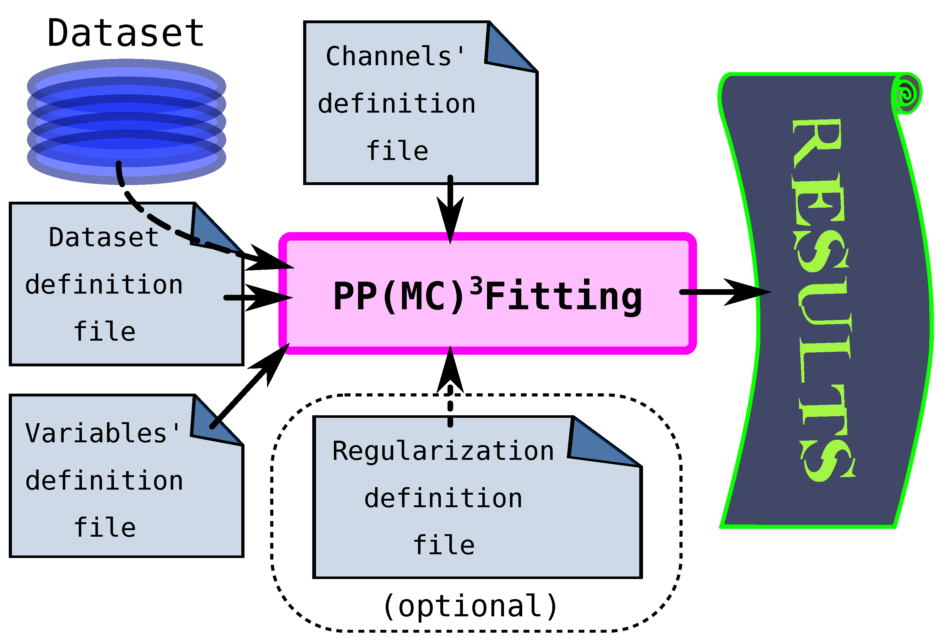
The first application of this algorithm was in Ref. [6] with generic Python scripts, but the development of general software for such fitting followed soon after. In the next section, we will discuss this software.

5. PP(MC ) 3 Fitting Software

The PP(MC ) 3 Fitting (pump–probe multichannel Markov chain Monte-Carlo fitting) is software that implements the algorithm from Section 4.4 for solving inverse problems of pump–probe spectroscopy. It is written in Python language and is composed of an application programming interface library libMCMCMCFitting.py and an actual script ppmc3fitting.py that provides communication with the user by a command line interface and a set of required and optional input files. The software also features a set of unit tests and basic examples of applications.
The general scheme of working with the PP(MC ) 3 Fitting software is given in Figure 6. There are three required input files for the software to work. The first one, the dataset definition file, provides the names of the files with the data that need to be fitted and the basis functions, which should represent the observables via Equation (76). The second input file, the channels’ definition file, provides the definition of the basis functions, i.e., which types of functions are there and which nonlinear variables they depend on. The last compulsory input file (variables’ definition file) initializes the nonlinear variables ( t 0 , τ cc , and τ r ): their minimal and maximal values, and optionally the initial value and the maximal step for the MC sampling routine. A fourth additional file is the regularization definition file, where additional constraints of the fitting can be defined. The data files are simple text files with three or four columns, where the first column provides the pump–probe delay, the second gives the yield of the observable, and the last column provides the yield uncertainty. The units of the first column of all data files define the time units of all corresponding nonlinear parameters.
The fitting procedure follows the algorithm described in Section 4.4. First, the local or global optimization is run on the data to find the minimum of the effective LSQ function (Equation (89)). For this, the minimization routines from the SciPy library are used [53]. The second step is MC sampling to obtain statistical estimates for the parameters. In the end, the program prints out both optimized and sampled values for nonlinear variables, Pearson correlation coefficients matrix, histograms for the variables, and also the numerical representation of the fitted function and the basis sets to plot alongside the fitted data. A more detailed application manual, the code itself, and examples of the fitting are provided in the electronic supporting information (ESI).
The software provides the following types of basis functions to fit pump–probe dynamics: “constant” ( B c , Equation (78)), “switch” ( B s , Equation (79)), “transient” ( B t , Equation (80)), and “Gaussian” ( B i , Equation (81)). The coherent oscillations functions (Equations (82) and (83)) were not implemented because these dynamics are not always present in the pump–probe data but require more parameters to be included, such as the oscillation frequency and the phase. Instead, the software also prints out the residuals of the fit, which will contain the oscillatory dynamics, if present. Therefore, the coherent oscillations can be fitted a posteriori from the fit, using Equations (82) and (83), similar to Ref. [8].
The PP(MC ) 3 Fitting software was successfully applied to disentangle complex dynamics of PAHs and published in Refs. [7,54,55]. For instance, in Ref. [7], a total of 31 decay times were extracted from the rich fragmentation dynamics of fluorene ( C 13 H 10 ), which corresponded to the lifetimes of the excited mono- and dications of this PAH molecule. Here, we will not show any complicated analysis, but rather provide a few numerical demonstrations of the capabilities of the PP(MC ) 3 Fitting software and of the approaches and concepts that could be used to work with the real-life experimental data.

6. Numerical Examples

6.1. Multiple Datasets with Shared Parameters

As a first example of the application of the PP(MC ) 3 Fitting software, we will consider the case of multiple datasets with shared parameters. For this, photoelectron sidebands will be used as an example [56]. We will base the discussion on the actual experimental pump–probe photoelectron spectra collected at the CAMP end-station [57,58] of the soft X-ray free-electron laser FLASH (DESY, Hamburg) [59,60] during the beamtime F-20191568. In this experiment, helium (He) atoms were pumped with XUV photons with an energy of h ν XUV = 40.8 eV (wavelength λ = 30.3 nm), produced by FLASH, and then probed by infrared (IR) photons with an energy of h ν IR = 1.5 eV ( λ = 810 nm). More details on the experiment can be found in Ref. [6].
He atoms resonantly absorb XUV photons with the energy of 40.8 eV, which is the He II line [61], producing an ionization event according to the reaction:
He + XUV He + + e ( KE 0 ) ,
where He + is the He monocation, e ( KE 0 ) is the photoelectron with kinetic energy of KE 0 = h ν XUV IP ( He ) = 16.2 eV, and IP ( He ) = 24.6 eV is the ionization potential of He [62].
However, in the presence of the IR strong field, the absorption or induced emission of photons by the ionized He can occur, leading to the gain or loss of the photoelectron energy, respectively, [56]. We can describe this process through the following reaction:
He + XUV ± n · IR He + + e ( KE n ) ,
where KE n = KE 0 ± n h ν IR is the new kinetic energy of the photoelectron, and n = , 1 , 0 , + 1 , is the number of the absorbed photons. If n = 0 , Equation (94) becomes Equation (93), producing photoelectrons with energy KE 0 , and this photoelectron line is also called a main line. However, if any IR photons are absorbed/emitted ( | n | > 1 ), then the photoelectron energy KE n KE 0 , and the resulting signal is called the sideband of the n-th order [56].
We can note that the sideband formation reaction (Equation (94)) is the same as the instant probing scheme (Equation (25)). Therefore, the temporal behavior of these photoelectron signals will be described with a basis function B i ( t pp ) (Equation (81)). Near the temporal overlap of both pulses ( t 0 ), the main line will be depleted, and the sidebands will be formed. According to the cross-correlation time expression (Equation (75)), we expect that the higher the sideband order | n | is, the smaller is the τ cc of this line. Furthermore, the sidebands should be symmetric, i.e., the width of the line at kinetic energy KE n should be the same as for KE n .
The experimental data (Figure 7) show exactly the behavior we described. We can extract the pump–probe photoelectron yields at given values of the photoelectrons’ kinetic energies KE n , corresponding to the intensities of the main line and the sidebands. From the data, in addition to the main line, we see sidebands of orders n = ± 1 , ± 2 , ± 3 , + 4 . All of these datasets can be fitted simultaneously with the PP(MC ) 3 Fitting software with a routine described in Section 4.4. The model function (Equation (76)) in all of the cases is given by:
F ( t pp t 0 ) = f c · B c ( t pp t 0 ) + f i · B i ( t pp t 0 ) ,
that is, it is a sum of the constant function B c = 1 (Equation (78)) describing the baseline and instant dynamic B i (Equation (81)). All eight datasets for the main line and seven sidebands share the parameter t 0 . The fit for all data should also have five cross-correlation time parameters τ cc ( n ) , with n = 0 , 1 , 2 , 3 , 4 denoting the main line ( n = 0 ) and sideband order ( n 1 ) according to Equation (94). Since the ± n sidebands are produced with the same amount of IR photons, they should have the same cross-correlation time.
We performed two types of fits: a global fit for all eight datasets and separate fits for the main line (Fit #0) and sidebands of each order (Fits #1 to #4). The results are shown in Figure 8 and Table 1. As one can see, generally, the parameters obtained from both the global fit and the separate fits agree. However, the global fit allows us to reduce the uncertainty for some parameters and avoid inconsistencies between the datasets (e.g., Fit #1 or Fit #4). This, in particular, leads to an unambiguous and precise definition of t 0 = 38.522 ± 0.001 ps that can be used in further analysis, similar to Ref. [6].

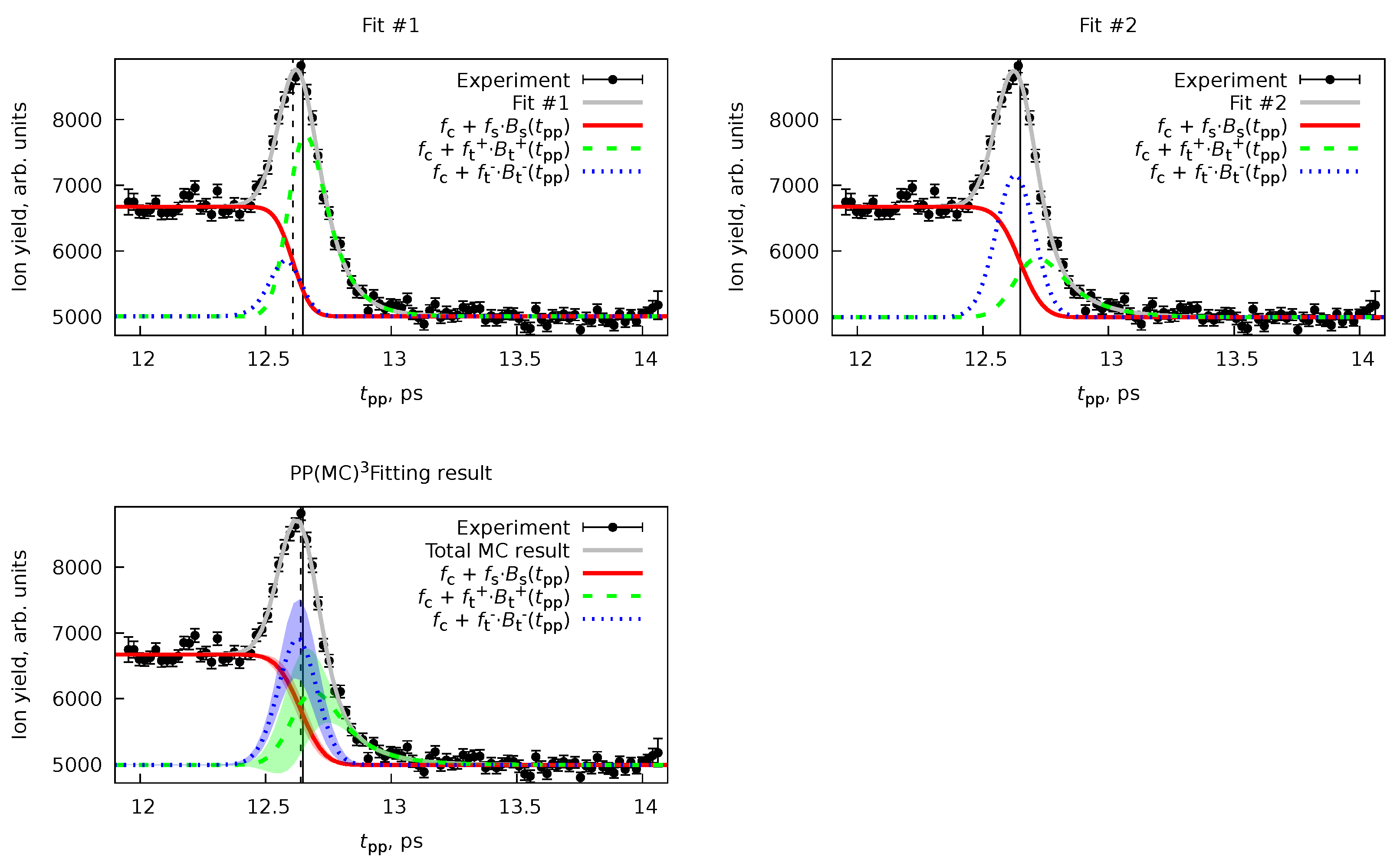
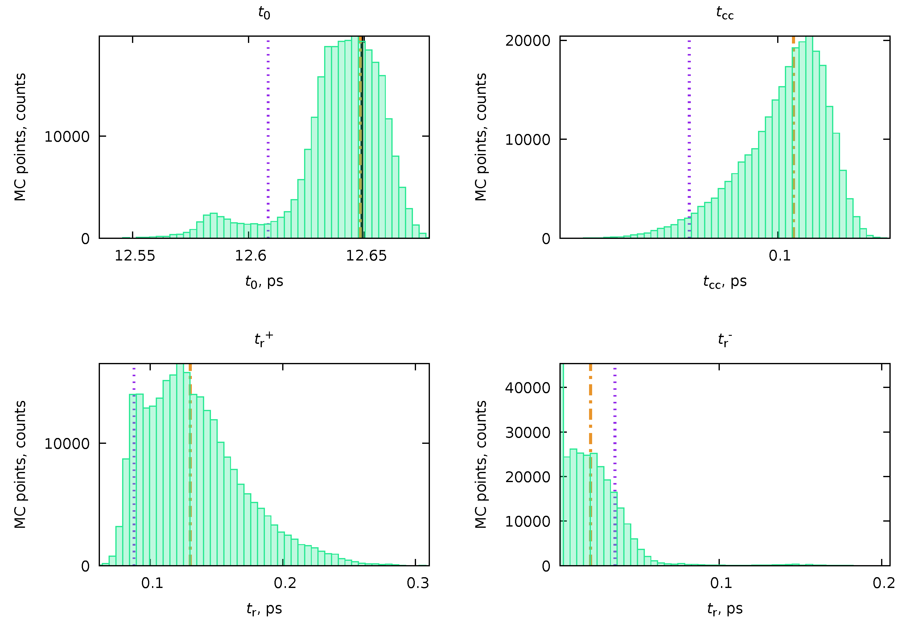
6.2. Forward-Backward Channel Dataset

Here, we will consider a case with two pump–probe channels, where the pump acts as a pump and the probe as a probe, and an inverted case, where the probe pulse acts as a pump, and the pump pulse acts as a probe. We will take the formation of the fluorene dication from Ref. [6] as an example. In that work, the neutral three-ring PAH fluorene ( C 13 H 10 ) was investigated in an XUV-IR pump–probe experiment with the same parameters as given in the previous Section 6.1. Upon a first look at the experimental ion yield of the fluorene dication C 13 H 10 2 + (Figure 9), one would think that there is a single transient peak and a switch function. However, the temporal overlap t 0 = 12.650 ± 0.005 ps determined with the help of helium sidebands [6], similar to that in Section 6.1, does not allow to fit the resulting behavior using a single transient. The simplest model to explain this anomaly is that the peak is composed of two transients: one with the XUV pulse acting as a pump and the second with the IR pulse acting as a pump.
The model (Equation (76)) proposed for the fitting of such a signal is the following:
F ( t pp t 0 ) = f c · B c ( t pp t 0 ) + + f s · B s ( t pp t 0 ) + f t + · B t + ( t pp t 0 ) + f t · B t ( t pp t 0 ) ,
where “switch” and transient functions use a single cross-correlation time τ cc , and two transients B t ± are described with rate constants τ r ± , where τ r + describes lifetime of an excited fluorene monocation C 13 H 10 + * and τ r describes the lifetime of an excited neutral fluorene C 13 H 10 * [6].
Simple fitting of Equation (96) to the experimental data given in Figure 9 is a good example of the ill-posed problem. To illustrate that, we performed two fits with two sets of initial values of nonlinear parameters t 0 , τ cc , τ r + , and τ r using the Marquardt–Levenberg algorithm [64,65] with the Gnuplot software [63]. The initial t 0 in both cases was taken as a value from the He sidebands, and the initial τ cc was taken from the MC result in Ref. [6]. The only difference is that the initial decay times were taken as 50 fs in the first fit, whereas in the second, they were 150 fs.
Figure 9 and Table 2 show results for both fits. The overall description of the data looks equivalent in both cases, but the actual values of the nonlinear parameters are quite different. While some of the parameters are equivalent to each other due to huge uncertainties, the τ r + have significantly different values, judging from the standard deviations computed according to Equation (10). The LSQ function values are equivalent in both cases, making these solutions indistinguishable, using, e.g., χ 2 -statistics [12] or various criteria, such as the Akaike information criterion [66]. However, even by looking at the components of the fit (Figure 9), we can be sure that these are two alternative solutions.
Applying the algorithm from Section 4.4 is especially advantageous in such cases, since we can automatically sample through all various equivalent solutions, providing an adequate statistical representation of the result. The results of the application of the PP(MC ) 3 Fitting software are also given in Figure 9 and Table 2. Although the total fit looks exactly the same as Fit #1 and Fit #2, the uncertainties of the individual transient components ( f t + · B t + ( t pp t 0 ) and f t · B t ( t pp t 0 ) ) are significant. By examining the distributions for individual nonlinear variables (Figure 10), we realize that the MC procedure sampled through many equivalent solutions, including Fit #1 and Fit #2. A more accurate and realistic solution can be obtained by applying regularization of t 0 with the value from He sidebands, similar to Ref. [6].

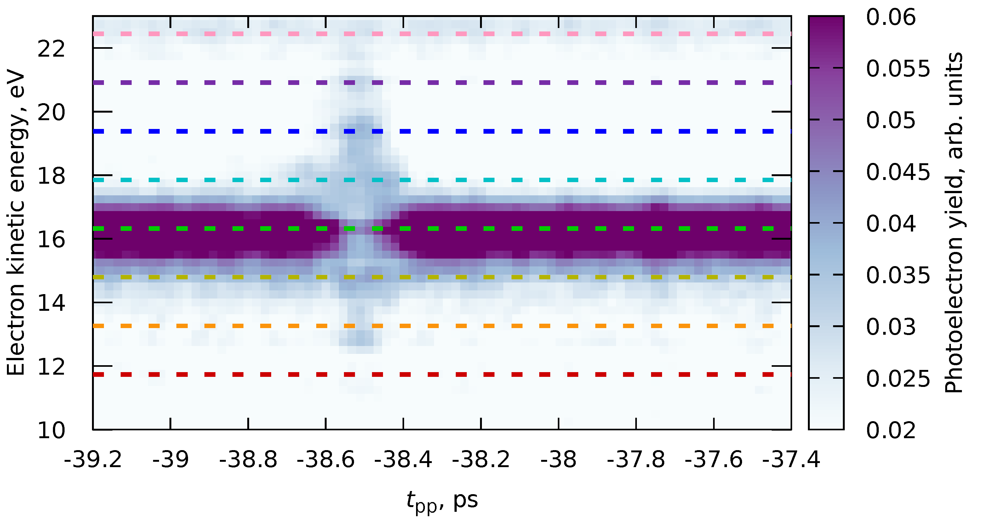
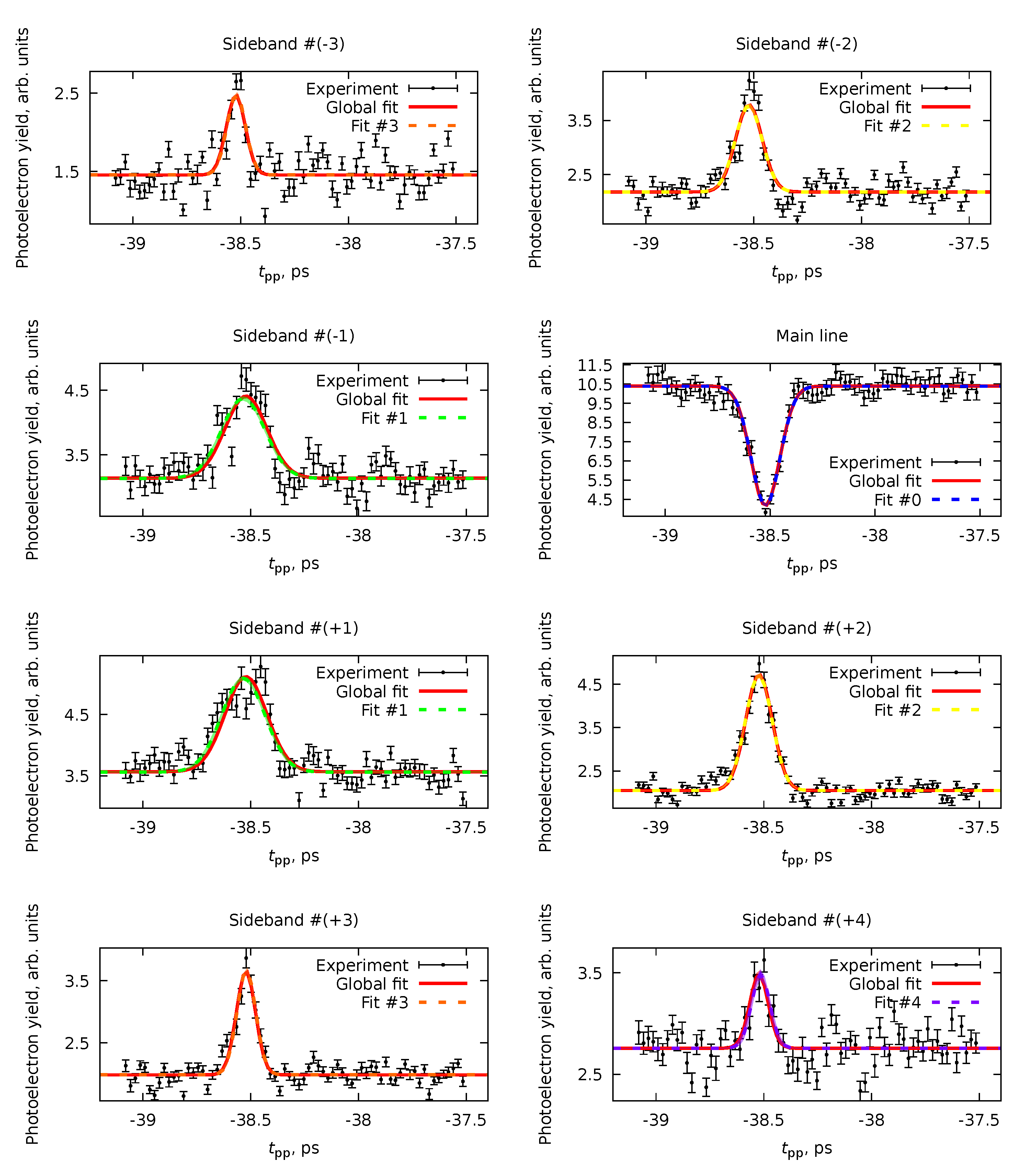
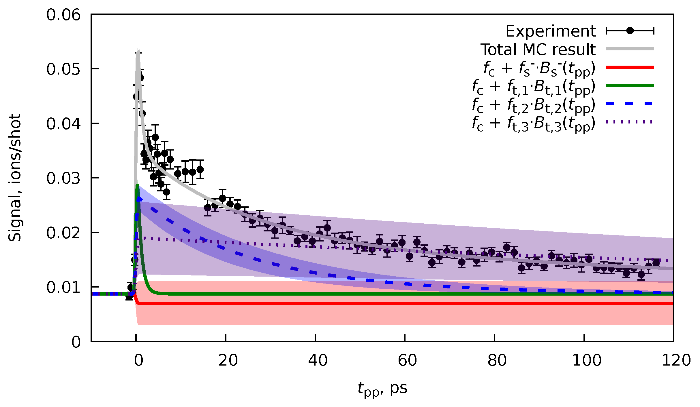
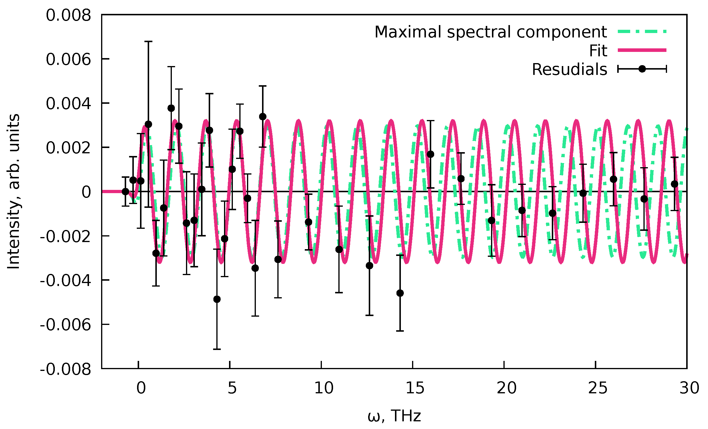
6.3. Treatment of the Data with Coherent Oscillations

As was said in Section 5, the PP(MC ) 3 Fitting software does not implement the basis functions for the coherent oscillations (Equations (82) and (83)). Nevertheless, this software can still be used to fit such datasets as well. As an example, we will use the ion yield of the indole-water ( C 8 H 7 N · H 2 O ) monocation from Ref. [10], where oscillatory dynamics were observed. In the original publication, a five-state model given by the Maxwell–Bloch equations was used, which produced three rate constants τ r , 1 = 0.45 ± 0.07 ps, τ r , 2 = 13 ± 2 ps, and τ r , 3 = 96 ± 10 ps, and also an oscillation frequency ω = 3.77 THz with phase φ = 1.77 .
To fit the same dataset for the indole-water monocation, we formulated an effective model with three effective decay times:
F ( t pp t 0 ) = f c · B c ( t pp t 0 ) + f s · B s ( t pp t 0 ) + i = 1 3 f t + · B t , i + ( t pp t 0 ) ,
where the t 0 was regularized with a value of t 0 , reg = 0 ± 1 fs, while all the rest of the nonlinear parameters τ cc and τ r , i ( i = 1 , 2 , 3 ), each from function B t , i , were left unregularized. The values of τ r , i were expected to be sufficiently different. Therefore, no repulsion regularization (Equation (92)) was applied in this case. Instead, the nonoverlapping regions for decay times were set: 0.01 τ r , 1 2 ps, 5 τ r , 2 40 ps, and 40 τ r , 3 300 ps. The resulting parameters obtained with PP(MC ) 3 Fitting were τ cc = 0.34 ± 0.02 ps, τ r , 1 = 0.9 ± 0.1 ps, τ r , 2 = 26 ± 5 ps, and τ r , 3 = 234 ± 34 ps. The obtained decay times are reasonably close to the ones obtained in Ref. [10] (see above), as well as to the experimentally estimated τ cc = 0.381 ps. An exact match was not expected since, in the original paper, a microscopic model was used, which produces the elementary rate constants, while our approach utilizes the effective rate constants.
The obtained fit (Figure 11) by design (Equation (97)) does not contain any of the oscillations, and this means that we have fitted only the noncoherent part of the signal (see Equations (51) and (57)). We can consider the fit’s residual to find the signal’s coherent part. The fit residual is defined as y = Y B p opt f opt (see Equations (86) and (87)) with the same uncertainties as of the original values. Since the desired oscillation signal is proportional to cos ( ω t + φ ) (Equations (51) and (57)), we can perform the Fourier transform (FT) of the residual part of the spectrum, to find the initial guess for the oscillation frequency ω and phase φ [12]. Since we know the residuals’ uncertainties and the dataset does not contain uniformly spaced data, instead of the fast FT algorithm [12], we can use a least-squares spectral analysis (LSSA) [67,67]. In particular, here, we used the regularized weighted LSSA (rwLSSA) introduced in Ref. [68] (see details in Appendix C). The rwLSSA spectrum of delay range of 0.7 t pp < 30 ps for a frequency range of 0 < ω 7 THz is shown in Figure 12. The maximal intensity is observed for a point of ω = 3.82 THz with phase φ = 1.4 at this point, which is already reasonably close to the parameters obtained in Ref. [10] ( ω = 3.77 THz and φ = 1.77 ).
We then performed a fit of the signal in the range 0.7 t pp < 10 ps with the highest density of points. We represented a signal as an oscillation function (Equation (82)):
f ( t pp ) = f o · B o ( t pp ) = f o 2 cos ( ω t pp + φ ) · 1 + erf t pp τ cc
with τ cc = 0.34 ps taken from the PP(MC ) 3 Fitting and rwLSSA peak parameters as initial conditions. By simple LSQ fitting, we get ω = 3.72 ± 0.05 THz and φ = 1.2 ± 0.3 . This result is shown in Figure 13. With that, we produced a full description of the pump–probe dataset for both the incoherent decay part of the signal and the coherent oscillations.
Now, we can summarize a universal analysis procedure that can be applied to the pump–probe datasets with the possible presence of coherent oscillations.
  • First, with the algorithm from Section 4.4 implemented in PP(MC ) 3 Fitting, we fit the nonoscillating part of the dynamics.
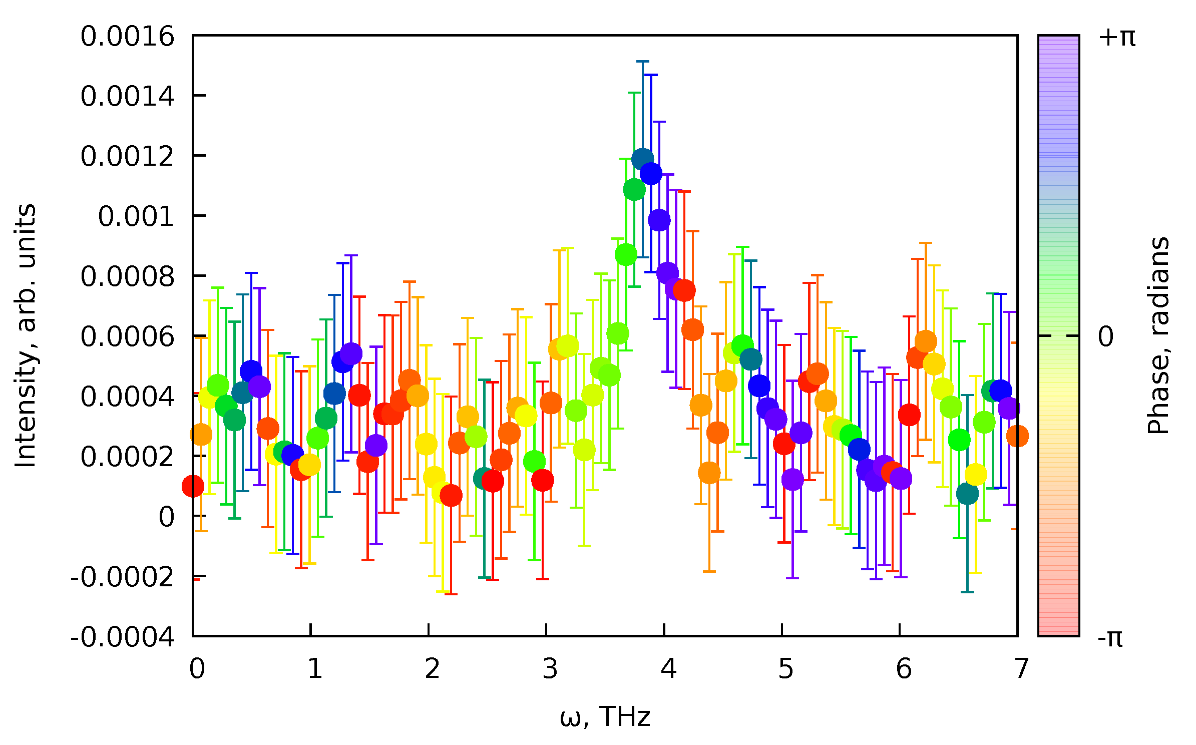
  • Then, we perform an rwLSSA analysis [68] (see Appendix C) for the residuals of the fit that are also printed by the PP(MC ) 3 Fitting. This analysis will allow us to check whether the signal contains any systematic oscillations. Note that the oscillations should be present only in t pp t 0 or in t pp 0 parts of the pump–probe data (see Equations (82) and (83)).
  • If the rwLSSA spectrum shows a presence of statistically meaningful oscillations in a reasonable range of frequencies, then the frequencies and the phases of the maximal amplitude signals from rwLSSA spectra can be used as initial guesses to fit the residuals of the PP(MC ) 3 Fitting result with expression Equation (76) and basis functions B o (Equation (82)) and B to (Equation (83)). Since the coherent oscillations should correspond to the incoherent processes, the cross-correlations and decay times from the PP(MC ) 3 Fitting results can be used.
The same procedure can also treat other unaccounted features in the experimental pump–probe data. One example is the presence of so-called coherent artifacts, which appear near the temporal overlap of the pump and probe pulses [69,70,71,72].

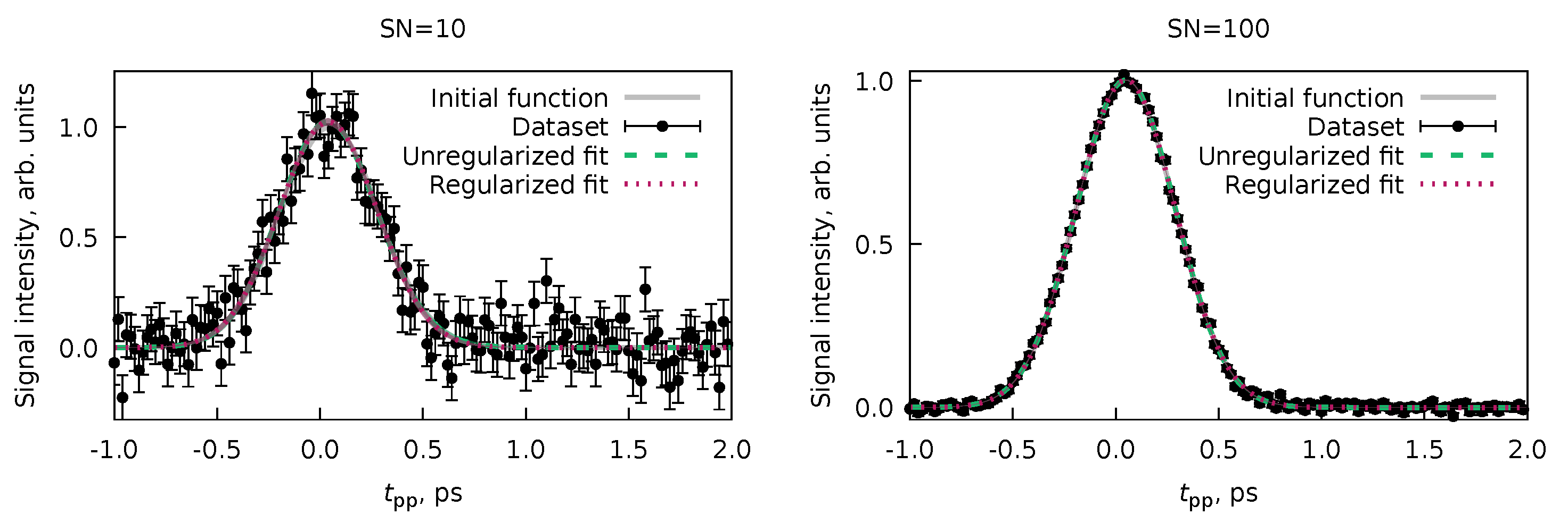
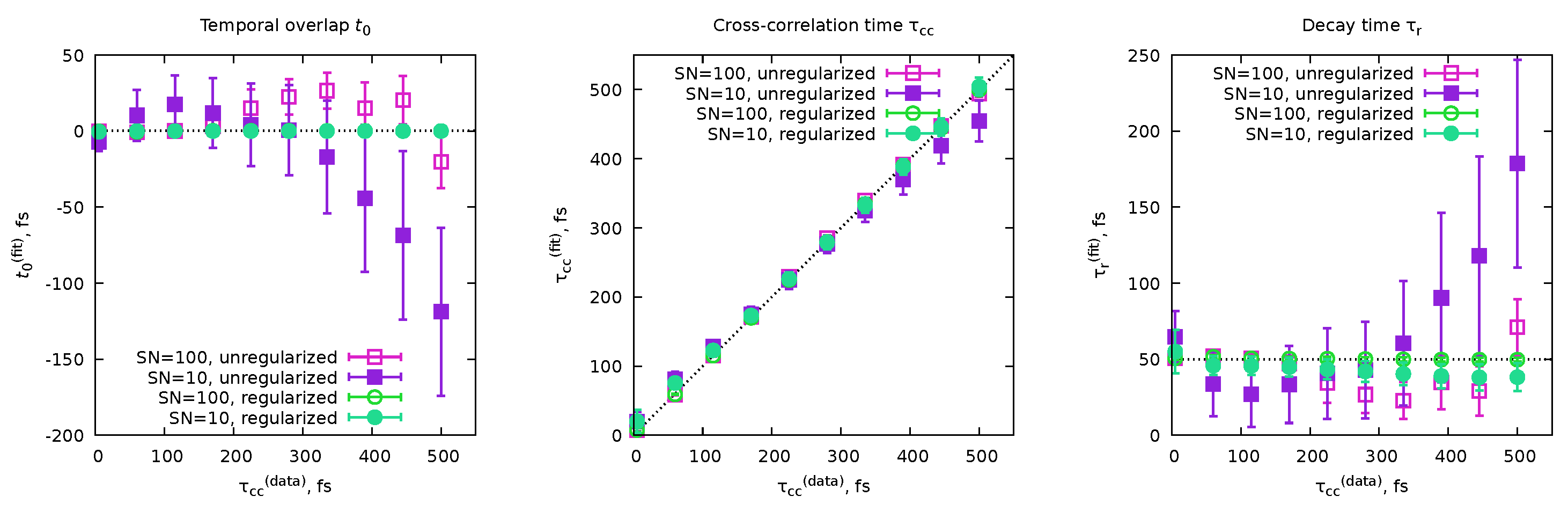
6.4. Cross-Correlation Time and Time Resolution

The last example we will show here is a demonstration of a concept rather than a PP(MC ) 3 Fitting demonstration. Sometimes, statements are shared that the “time resolution of pump–probe experiments is limited by the cross-correlation time” [11]. This leads to frequent questions about whether the rate constants extracted from the fits are smaller than the cross-correlation times of the experiments. However, such a direct application of the idea that the cross-correlation time is the limit for the shortest obtainable decay lifetimes is questionable since there are a few common ways to express both the cross-correlation time (Equation (71)) and the decay time (Equation (30)). Therefore, in this section, we decided to use the MC sampling of the possible solutions with PP(MC ) 3 Fitting to demonstrate the actual relation between the rate constants and the cross-correlation time.
To do that, we generated two sets of ten generic pump–probe data with a fixed decay time τ r = 50 fs, but with varied cross-correlation time 5 τ cc 500 fs. The upper limit was determined by the capabilities of the standard methods to represent the transient function B t ( t pp ) (Equation (80)). The standard methods, using SciPy [73] packages, allow for stable and smooth data produced for the ratios τ cc / τ r up to τ cc / τ r < 50 (see Appendix D). Such implementation of the B t ( t pp ) function is used in PP(MC ) 3 Fitting, but we limited ourselves to τ cc / τ r 10 .
All generated pump–probe data span the delays in the range 1 t pp + 2 ps with a step of 20 fs. Each set of data had a given signal-to-noise ratio (SN): one set had SN = 10 (high noise data), and the other SN = 100 (low noise data). Figure 14 shows an example of such data. Each of the datasets with a given τ cc and SN parameters was fitted with PP(MC ) 3 Fitting with the same function that it was generated with (Equation (80)), that is:
F ( t pp ) = f t · B t ( t pp ) .
Two fits were performed for each pump–probe dataset with a given τ cc and SN: without regularization and with regularization for t 0 with t 0 , reg = 0 ± 1 fs (see Figure 14).
The resulting trends for the three nonlinear parameters of the fit ( t 0 , τ cc , and τ r ) are shown in Figure 15. As we can see, for the fully unregularized fit with SN = 10, the procedure gives reasonable results (see also Figure 15) up to τ cc 300 fs ( τ cc / τ r = 6 ). At a lower noise level (SN = 100), reasonable results extend to around τ cc 450 fs ( τ cc / τ r = 9 ). Upon applying the regularization, both the low noise level (SN = 100) and high noise level (SN = 10) fits were able to reproduce the preset parameters up to τ cc = 500 fs. Therefore, we can conclude that the decay times (Equation (30)) can be reliably fitted below the value of the cross-correlation time (Equations (5) and (75)) with a single dataset. The lower noise level and preliminary knowledge of the parameters, such as the position of the temporal overlap ( t 0 ), allow shorter decay times to be reliably fitted. Combining the datasets in a global fit, as shown in Section 6.1, can also be used to increase the accuracy of the results.

7. Conclusions

In this manuscript, we extensively discussed the inverse problem solution (fitting) for the pump–probe spectroscopic datasets. We examined the theoretical aspects of the inverse problem solution and the standard model used to fit the pump–probe data. Here, we provided rigorous proof that the classical set of model functions used to fit the pump–probe experimental data is sufficient to describe any pump–probe observables, given that only first-order reactions are possible (Appendix A.8). In addition, we have extended the standard set of the basis functions used to fit the pump–probe dynamics with two additional ones, describing coherent oscillations in the dataset (Equations (82) and (83)).
We proposed a general-purpose algorithm for treating the inverse problem of the pump–probe spectroscopy (outlined in Section 4.4). In short, it is based on separating the linear and nonlinear parameters. First, a global fit of the data is performed, and then the uncertainties of the fitted parameters are determined by the Markov chain Monte-Carlo routine. This approach was implemented in the Python software PP(MC ) 3 Fitting, which can be used in a standardized fashion for various datasets. With the numerical examples, we highlighted the common ideas for application, such as global fits with shared parameters between different datasets, the presence of parasitic channels, and stepwise treatment of the coherent oscillations in the data. We also commented on a commonly misdiscussed issue of the time resolution in the pump–probe spectroscopy.
The presented PP(MC ) 3 Fitting software is a complementary addition to the existing methods used to analyze experimental pump–probe data. Examples of such approaches include global and target analysis [32,38,74], KiMoPack [33], lifetime density maps analysis [75,76,77], and Maxwell–Bloch equation modeling [4,34]. Adding the PP(MC ) 3 Fitting to the listed set of methods can be useful for the ultrafast community to robustly and effectively tackle complicated experimental pump–probe results with various dynamical observables (Supplementary Materials).

Supplementary Materials

The following supporting information can be downloaded at: https://www.mdpi.com/article/10.3390/photochem4010005/s1, The presented software is a complementary addition to the existing methods used to analyze experimental pump-probe data.

Author Contributions

Conceptualization, D.S.T. and M.S.; methodology, D.S.T. and D.G.; software, D.S.T. and D.G.; validation, D.S.T. and D.G.; formal analysis, D.S.T. and D.G.; investigation, D.S.T. and D.G.; resources, M.S.; data curation, D.S.T. and M.S.; writing—original draft preparation, D.S.T.; writing—review and editing, M.S. and D.G.; visualization, D.S.T.; supervision, M.S.; project administration, M.S.; funding acquisition, M.S. All authors have read and agreed to the published version of the manuscript.

Funding

This research received no external funding.

Data Availability Statement

The latest versions (at date of manuscript preparation) of the PPM C 3 Fitting code, manual, and numerical examples shown in the article are available in the Electronic Supporting Information. The latest version of the PPM C 3 Fitting code is available at https://gitlab.desy.de/denis.tikhonov/mcmcmcfitting/ (accessed on 18 January 2024).

Acknowledgments

This work has been supported by Deutsches Elektronen-Synchtrotron DESY, a member of the Helmholtz Association (HGF).

Conflicts of Interest

The authors declare no conflicts of interest.

Abbreviations

The following abbreviations are used in this manuscript:
FELFree-electron laser
FTFourier transform
IRInfrared
LSQLeast-squares
(rw)LSSA(Regularized weighted) least-squares spectral analysis
MCMonte-Carlo
PAHPolycyclic aromatic hydrocarbon
SNSignal-to-noise ratio
XUVExtreme ultraviolet

Appendix A. Detailed Derivations of Delta-Shaped Pump–Probe Dynamics

Appendix A.1. Solution of the First-Order Kinetics Equations

We are solving Equation (28) of the following form ( [ A * ] = y , k r = k ):
y ˙ = d y d t = k y
for function y = y ( t ) with initial condition y ( 0 ) = y 0 . Let us rewrite this equation as:
d y y = k d t
and integrate the left part from y 0 to y ( t ) and the right part of the same equation from 0 to t as:
y 0 y ( t ) d y y = ln y ( t ) y 0 = k 0 t d t = k t .
Rearranging this result, we obtain the final solution of the form:
y ( t ) = y 0 · exp ( k t ) ,
as given in Equation (29).
Now, we integrate Equation (31) for the product of the decay ( [ C ] = z ) with substituted Equation (A2), which gives:
z ˙ = k y = k y 0 · exp ( k t ) .
Such an equation can simply be integrated in time from 0 to t with the initial condition z ( 0 ) = 0 as:
0 t z ˙ d t = z ( t ) = k y 0 0 t exp ( k t ) d t = y 0 1 exp ( k t ) .

Appendix A.2. Coherent Quantum Dynamics without Decay

We start from the von Neumann Equation (Equation (41)):
i ϱ ˙ = [ H , ϱ ] = H ϱ ϱ H ,
where the density matrix ϱ (Equation (38)) and Hamiltonian matrix H (Equation (42)) are:
ϱ = ρ 00 ρ 01 ρ 10 ρ 11 , H = ω 0 0 0 1 .
where ϱ ˙ is a matrix, composed of elements ρ ˙ k l ( k , l = 0 , 1 ). By computing two products of these matrices, we obtain:
H ϱ = ω 0 0 ρ 10 ρ 11 and ϱ H = ω 0 ρ 01 0 ρ 11 .
Substitution of these results in the initial equation results in a matrix equation:
i ρ ˙ 00 ρ ˙ 01 ρ ˙ 10 ρ ˙ 11 = ω 0 ρ 01 + ρ 10 0 .
We can rewrite this equation as a system of equations for corresponding individual matrix elements from the left and right sides:
i ρ ˙ 00 = 0 , i ρ ˙ 01 = ω ρ 01 , i ρ ˙ 11 = 0 , i ρ ˙ 10 = + ω ρ 10 .
By dividing the left and right sides by i , we arrive at Equations (43). First, let us integrate the equations, describing the dynamics of the diagonal elements ( ρ 00 and ρ 11 ) with initial conditions (Equation (40)) of ρ 00 ( 0 ) = 1 p and ρ 11 ( 0 ) = p :
1 p ρ 00 ( t ) ρ ˙ 00 d t = ρ 00 ( t ) ( 1 p ) = 0 0 t d t = 0 ρ 00 ( t ) = 1 p , p ρ 11 ( t ) ρ ˙ 11 d t = ρ 11 ( t ) p = 0 0 t d t = 0 ρ 11 ( t ) = p .
For off-diagonal elements, the rate equations have the same form as Equation (A1) ( y = ρ 01 , ρ 10 and k = i ω ). Thus, the solution is given with Equation (A2), that is:
ρ 01 ( t ) = ρ 01 ( 0 ) · exp ( + i ω t ) , ρ 10 ( t ) = ρ 10 ( 0 ) · exp ( i ω t ) .
Taking into account the initial conditions (Equation (40)) of ρ 01 ( 0 ) = p · ( 1 p ) exp ( + i φ ) and ρ 10 ( 0 ) = p · ( 1 p ) exp ( i φ ) , we arrive at:
ρ 01 ( t ) = p · ( 1 p ) · exp ( + i φ + i ω t ) , ρ 10 ( t ) = p · ( 1 p ) · exp ( i φ i ω t ) .

Appendix A.3. Relation between Quantum and Classical Regimes

The classical incoherent regime in coherent regimes (Equation (51) or (57)) appears as a result of incoherent excitation. For instance, such an incoherent regime can appear when different molecules have different imprinted phases φ from the pump pulse. In this case, we need to average all these signals from all the incoherent molecules. Let us assume that the following expression gives the result of a molecule with an imprinted phase φ :
f ( t pp , φ ) = F 0 ( t pp ) + F 1 ( t pp ) · cos ( ω t + φ ) ,
where F 0 ( t pp ) is the phase-independent part of observable and F 1 ( t pp ) is the oscillation prefactor. Both Equations (51) and (57) can be reduced to such a form. The distribution of the molecules with various oscillation phases φ will be given by a probability distribution P ( φ ) , normalized as 0 2 π P ( φ ) d φ = 1 . In this case, the result of the ensemble observation will be:
f ( t pp ) = 0 2 π f ( t pp , φ ) P ( φ ) d φ .
If we now assume that all phases are equally possible, i.e., P ( φ ) is a uniform distribution for φ [ 0 ; 2 π ) ( P ( φ ) = ( 2 π ) 1 ), then we get an averaging result:
f ( t pp ) = 1 2 π 0 2 π f ( t pp , φ ) d φ = = F 0 ( t pp ) · 1 2 π 0 2 π d φ 2 π + F 1 ( t pp ) · 1 2 π 0 2 π cos ( ω t + φ ) d φ 0 = F 0 ( t pp ) .
In other words, the oscillating observables disappear, and only the nonoscillating incoherent part of the signal is left. This result can also be obtained by setting the nondiagonal elements to zero in the density matrix in Equation (47), which is known to lead to a classical regime of the quantum system [78,79].

Appendix A.4. Coherent Quantum Dynamics with Decay

The initial Linblad Equation (52) has the following form:
i ϱ ˙ = [ H , ϱ ] + i γ σ ϱ σ + 1 2 { σ + σ , ϱ } = = H ϱ ϱ H + i γ σ ϱ σ + 1 2 σ + σ ϱ 1 2 ϱ σ + σ .
The σ ± matrices (Equation (53)) are the excitation/deexcitation operators. If we represent the system’s wavefunction | ψ = c 0 | 0 + c 1 | 1 with a vector of coefficients ( c 0 , c 1 ) , and apply σ ± for states | 0 and | 1 , described as ( 1 , 0 ) and ( 0 , 1 ) , respectively, then we get:
σ + | 0 = 0 0 1 0 1 0 = 0 1 = | 1
and
σ | 1 = 0 1 0 0 0 1 = 1 0 = | 0 .
To get the matrix equation for the system evolution, we need to calculate the additional term i γ σ ϱ σ + ( 1 / 2 ) · { σ + σ , ϱ } of Equation (A5), which describes the decay in the quantum system. For this, we evaluate each of the following components:
σ ϱ σ + = 0 1 0 0 ρ 00 ρ 01 ρ 10 ρ 11 0 0 1 0 = ρ 11 0 0 0 ,
σ + σ ϱ = 0 0 1 0 0 1 0 0 ρ 00 ρ 01 ρ 10 ρ 11 = 0 0 ρ 10 ρ 11 ,
and
ϱ σ + σ = ρ 00 ρ 01 ρ 10 ρ 11 0 0 1 0 0 1 0 0 = 0 ρ 01 0 ρ 11 .
Substituting these matrices into Equation (A8) with the previously evaluated first part (Equation (A6)), we get:
i ρ ˙ 00 ρ ˙ 01 ρ ˙ 10 ρ ˙ 11 = ω 0 ρ 01 + ρ 10 0 + i γ + ρ 11 1 2 ρ 01 1 2 ρ 10 ρ 11 .
From this matrix equation, we can obtain a modified set of Equations (A7):
i ρ ˙ 00 = + i γ ρ 11 , i ρ ˙ 01 = ω ρ 01 i γ 2 ρ 01 , i ρ ˙ 10 = + ω ρ 10 i γ 2 ρ 10 . i ρ ˙ 11 = i γ ρ 11 .
Dividing these equations by i , for elements ρ 01 , ρ 10 , and ρ 11 , we arrive to the decay differential equations (Equation (A1)) with k = γ / 2 i ω , k = γ / 2 + i ω , and k = γ , respectively. This results in the solution given by Equation (A2) with corresponding decay rates. A similar procedure for ρ 00 leads to an Equation (A3) with k = γ , which leads to the solution in Equation (A4). All these results are summarized in Equation (55) in the main text.

Appendix A.5. Reaction Scheme with Multiple Products

Let us consider the reaction scheme (a) from Figure 4, which can be represented with the following system of chemical reactions:
M + pump A * A * k 1 C 1 A * k 2 C 2 A * k N C N A * + probe B .
It can be considered as an extension of scheme (27) with N various decay results C 1 , C 2 , , C N . We will denote [ A * ] = y ( [ A * ] ( 0 ) = y ( 0 ) = y 0 ) and [ C i ] = z i ( i = 1 , , N ). In this case, the rate equation for A * will be:
y ˙ = i = 1 N k i k eff y = k eff y .
This rate equation is the same Equation (A1) with solution (A2). For each of the products C i , the rate equations are:
z i ˙ = + k i · y = k i · y 0 · exp ( k eff t ) ,
which is the same as Equation (A3). Thus, the solution for product C i is given by Equation (A4). From this, the pump–probe dynamics of [ B ] and [ C ] are given by Equation (33). Since we can express rate constants through the decay lifetimes ( k i = τ i 1 , see Equation (30)), we can express the effective rate constant as:
τ r = 1 i = 1 N k i k eff = i 1 τ i 1 .

Appendix A.6. Reaction Scheme with Sequential Metastable Intermediates

Let us consider the reaction scheme (b) from Figure 4, which can be represented with the following system of chemical reactions:
M + pump A 1 * A 1 * k 1 A 2 * A 2 * k 2 A 2 * + probe B ,
where we get the formation of the intermediate A 1 * by the pump, which is followed by the decay into A 2 * , which in turn decays further. The probing is done using B. First, we solve rate equation for [ A 1 * ] = y 1 :
y ˙ 1 = k 1 y 1 ,
which is Equation (A1) with solution (Equation (A2)):
y 1 ( t ) = y 1 ( 0 ) y 10 · exp ( k 1 t ) = y 10 · exp ( k 1 t ) .
The rate equation for [ A 2 * ] = y 2 looks as follows:
y ˙ 2 = + k 1 y 1 k 2 y 2 ,
which can be thought of as a combination of Equations (A1) and (A3). Thus, we can try to find the solution as a combination of (A2) and (A4) as:
y 2 ( t ) = α 1 exp ( k 1 t ) + α 2 exp ( k 2 t ) ,
where α 1 and α 2 are coefficients. By applying a boundary condition y 2 ( 0 ) = 0 , we get α 1 = α 2 . Then, substituting (A11) and (A9) into (A10), we get:
α 1 · exp ( k 1 t ) · ( k 2 k 1 ) = y 10 · k 1 · exp ( k 1 t ) .
Dividing this equation by exp ( k 1 t ) · ( k 2 k 1 ) , we get:
α 1 = α 2 = y 10 · k 1 k 2 k 1 ,
which results in:
y 2 ( t ) = y 10 · k 1 exp ( k 1 t ) exp ( k 2 t ) ( k 2 k 1 ) .
The yield of B at t pp < 0 is zero, and at t pp 0 it is [ B ] ( t pp ) = p · y 2 ( t pp ) , where p is the probing efficiency (similar to Equation (33)). This gives the following pump–probe yield of B:
[ B ] ( t pp ) = p · y 10 · k 1 ( k 2 k 1 ) · θ ( t pp ) · exp ( k 1 t ) exp ( k 2 t ) .

Appendix A.7. Reaction Scheme with Multiple Intermediates Forming a Single Product

Let us consider the reaction scheme (c) from Figure 4, which can be represented with the following system of chemical reactions:
M + pump A 1 * M + pump A 2 * A 1 * k 1 C A 2 * k 2 C A 1 * + probe B 1 A 2 * + probe B 2 .
The kinetic equations for [ A i * ] = y i ( i = 1 , 2 ) are the following ones:
y ˙ i = k i y i ,
which are the decay Equation (A1), with the solution (Equation (A2)) given as:
y i ( t ) = y i 0 · exp ( k i t ) ,
where y i 0 = y i ( 0 ) are the initial amounts of A 1 * and A 2 * created by the pump pulse. This solution (similar to Equation (33)) provides the amount of B i as a function of the pump–probe delay t pp to be:
[ B i ] ( t pp ) = p i · y i 0 · θ ( t pp ) · exp ( k i t ) ,
where p i is the conversion efficiency of A i * into B i by the probe pulse.
The rate equation for [ C ] = z is as follows:
z ˙ = + k 1 y 1 + k 2 y 2 = k 1 y 10 · exp ( k 1 t ) + k 2 y 20 · exp ( k 2 t ) ,
which can be solved by direct integration with boundary condition z ( 0 ) = 0 as:
0 t z ˙ d t = z ( t ) = k 1 y 10 · 0 t exp ( k 1 t ) d t + k 2 y 20 · 0 t exp ( k 2 t ) d t = y 10 ( 1 exp ( k 1 t ) ) + y 20 ( 1 exp ( k 2 t ) ) .
At t , z ( t ) y 10 + y 20 . At t pp < 0 , the yield of C is given as [ C ] ( t pp ) = y 10 + y 20 . At t pp 0 , it is going to be the amount of full conversion ( y 10 + y 20 ) without the amount lost for B 1 and B 2 with a probe (Equation (A12)). Therefore, the total amount of C can be written (similar to Equation (33)) as:
[ C ] ( t pp ) = i = 1 2 y i 0 p i · y i 0 · θ ( t pp ) · exp ( k i t ) .

Appendix A.8. General form of the Decay Dynamics Pump–Probe Equations

Now, we will consider the generalized version of the decay reaction dynamics, described in Section 3.2 of the main text and Appendixes Appendix A.5, Appendix A.6, and Appendix A.7 of the Appendix. Let us consider that we have N compounds A 1 , A 2 , , A N , formed by the pump from the initial molecule M and/or those formed by the probe pulse from the species formed by the pump pulse. The amount of each of compound A i will be denoted as y i . An N-dimensional vector describing the current amounts of all compounds will be denoted as:
y = y 1 y 2 y N ,
where the pump pulse forms the initial distribution of states y 0 .
The system of reaction equations for free evolution of the system will be the following:
A 1 k 1 2 s 1 2 · A 2 A 1 k 1 3 s 1 3 · A 3 A i k i j s i j · A j A N k N N 1 s N N 1 · A N 1 .
where we consider all possible reactions of decay into each other ( 1 i , j N and i j ) with rate constants k i j 0 and stoichiometric coefficients s i j 0 , where k i j = 0 and s i j = 0 mean that this reaction is not happening. The free evolution of the system is, thus, given by the following rate equation:
y ˙ = K y ,
where matrix K consists of the following elements. The diagonal elements K i i are given as:
K i i = + j = 1 , j i N k i j ,
while the off-diagonal elements are defined as:
K j i = s i j · k i j .
To obtain the solution of Equation (A13) [12], we will consider the solutions to the following eigenproblem:
K u i = γ i u i .
All eigenvalues should be nonnegative for physically-relevant reaction schemes ( γ i 0 ). From a set of N orthonormal eigenvectors u i ( i = 1 , , N and u i T u j = δ i j ), we can form a matrix of orthogonal transformation:
U = ( u 1 , u 2 , , u N ) .
We can now diagonalize matrix K as:
Γ = U K U T = diag ( γ 1 , γ 2 , , γ N ) .
Now, we can replace y and y ˙ with Y = U y and Y ˙ = U y ˙ by multiplying Equation (A13) with U from the left side:
Y ˙ = U y ˙ = U K U T U E y = Γ Y ,
where E is an N × N identity matrix. The solution for this equation is:
Y ( t ) = exp ( Γ · t ) Y 0 ,
where Y 0 = U y 0 is the initial condition and the exponential matrix exp ( Γ · t ) is:
exp ( Γ · t ) = diag ( exp ( γ 1 t ) , exp ( γ 2 t ) , , exp ( γ N t ) ) .
We can go back to y = U T Y by multiplying this solution with U T from the left, resulting in:
y ( t ) = U T exp ( Γ · t ) U T ( t ) y 0 = T ( t ) y 0 ,
where T ( t ) is the free evolution operator. If we expand each of the components y i , we get:
y i ( t ) = j = 1 N c i j exp ( γ j t ) ,
where the dynamics of each of the components is a sum of exponential decays with effective rate constants (for γ j > 0 ) and static yields (for γ j = 0 ) with constant coefficients c i j that depend on the initial conditions y 0 and on the reaction scheme.
To describe the probe process, we will also consider another set of rate equations:
A 1 + probe p 1 2 s 1 2 A 2 A 1 + probe p 1 3 s 1 3 A 3 A i + probe p i j s i j A j A N + probe p N N 1 s N N 1 A N 1 ,
where 0 p i j 1 describe the probing efficiency of a given process and s i j 0 are the stoichiometric coefficients ( p i j = 0 and s i j = 0 mean that this process does not happen). Therefore, we can describe probing at time t > 0 as an instant shuffling of the products as replacement current values y ( t ) with P y ( t ) , that is:
y ( t ) P y ( t )
where the matrix P has the following nondiagonal elements:
P j i = s i j · p i j
and diagonal elements:
P i i = j = 1 , j i N ( 1 p i j ) .
At t pp < 0 , the system continues a free evolution until the detection. Therefore, we can describe the observable yield of all the components f ( t pp ) as:
f ( t pp ) = lim t y ( t ) = lim t T ( t ) T y 0 = T y 0 ,
where T is given as:
T = U T diag ( θ ( γ 1 ) , θ ( γ 2 ) , , θ ( γ N ) ) lim t exp ( Γ · t ) U ,
where for γ i = 0 we get θ ( γ i ) = 1 and for γ i > 0 we get θ ( γ i ) = 0 .
At t pp > 0 , we get a free evolution from the initial conditions y 0 , then the action of the probe according to Equation (A14), and then again free evolution until detection. We can write this (similar to Equation A15) as:
f ( t pp ) = T P T ( t pp ) y 0 .
Combining Equations (A15) and (A16), we get the following equation describing all the pump–probe yields of all products:
f ( t pp ) = T · E + θ ( t pp ) · P T ( t pp ) E y 0 .
For each of the compounds A i , their pump–probe yield can be described as:
f i ( t pp ) = q 0 + j = 1 N q i · θ ( t pp ) · exp ( γ i t pp ) ,
where q j ( j = 0 , 1 , , N ) are the coefficients related to initial conditions y 0 , reaction scheme, and also probing efficiencies. Terms with exponents appear from the operator T ( t pp ) in the expression above.

Appendix B. Effects of the Duration of the Pulses and Experimental Setup Jitter

Appendix B.1. Sequential Convolution with Gaussian-Shaped Pulses

Let us consider a sequential convolution of the following form:
f p 1 p 2 = = 1 π τ 1 τ 2 + + f ( t t 1 t 2 ) · exp t 1 2 τ 1 2 d t 1 · exp t 2 2 τ 2 2 d t 2 ,
where f ( t ) is some arbitrary function, and p i ( t ) ( i = 1 , 2 ) are the normal distributions:
p i ( t ) = 1 π · τ i · exp t i 2 τ i 2 .
Trying to simplify Equation (A17), we can replace variables t 1 and t 2 with:
T = t 1 + t 2 , q = t 2 t 1 , i . e . , t 1 = T q 2 , t 2 = T + q 2 .
The Jacobian J for such transformation is:
J = det t 1 T t 2 T t 1 q t 2 q = det + 1 / 2 + 1 / 2 1 / 2 + 1 / 2 = 1 2 ,
which means that d t 1 d t 2 = J d T d q = 1 2 d T d q . Substitution of coordinates from Equation (A18) into Equation (A17) results in:
f p 1 p 2 = = 1 2 π τ 1 τ 2 + f ( t T ) + exp ( T q ) 2 4 τ 1 2 ( T + q ) 2 4 τ 2 2 d q I ( T ) d T ,
and therefore, we only need to evaluate the integral I ( T ) . First, let us rearrange the expression inside the exponent as:
( T q ) 2 4 τ 1 2 ( T + q ) 2 4 τ 2 2 = = ( τ 1 2 + τ 2 2 ) 4 τ 1 2 τ 2 2 · T 2 + q 2 2 ( τ 2 2 τ 1 2 ) ( τ 1 2 + τ 2 2 ) · T a · q = = ( τ 1 2 + τ 2 2 ) 4 τ 1 2 τ 2 2 · T 2 + q 2 2 · a · q + a 2 a 2 = = ( τ 1 2 + τ 2 2 ) 4 τ 1 2 τ 2 2 · 1 ( τ 2 2 τ 1 2 ) 2 ( τ 1 2 + τ 2 2 ) 2 · T 2 ( τ 1 2 + τ 2 2 ) 4 τ 1 2 τ 2 2 · ( q a ) 2 = = T 2 τ 12 2 ( q a ) 2 τ q 2 ,
where
τ 12 2 = τ 1 2 + τ 2 2
and
τ q 2 = 4 τ 1 2 τ 2 2 ( τ 1 2 + τ 2 2 ) = 4 τ 1 2 τ 2 2 τ 12 2 .
Substitution of the result from Equation (A20) into I ( T ) from Equation (A19) results in:
I ( T ) = + exp ( T q ) 2 4 τ 1 2 ( T + q ) 2 4 τ 2 2 d q = = exp T 2 τ 12 2 · + exp ( q a ) 2 τ q 2 d q = π τ q · exp T 2 τ 12 2 = = 2 π τ 1 τ 2 τ 12 · exp T 2 τ 12 2 ,
which upon substitution into Equation (A19) and replacement of T = t 12 provides us a final answer of:
f p 1 p 2 = 1 π τ 12 + f ( t t 12 ) · exp t 12 2 τ 12 2 d t 12 .
In other words, convolution of function f ( t ) with two Gaussian functions is equivalent to convolution with a single effective Gaussian function:
f 12 ( t ) = 1 π τ 12 exp t 2 τ 12 2 ,
where the effective width τ 12 2 is given by Equation (A21). If we require the calculation of a triple convolution, we can apply this result sequentially as:
f p 1 p 2 f p 12 p 3 = f p 123 ,
where the final effective Gaussian function p 123 ( t ) will have the effective width τ 123 2 = τ 1 2 + τ 2 2 + τ 3 3 . Such a process can be continued for any arbitrary number of Gaussian functions, yielding the result listed in Equation (72).

Appendix B.2. Basis Functions for Fitting Observables with Finite Duration Pump/Probe Pulses and Experimental Jitter

Here, we explicitly calculate the convolution of the basis functions b x ( x = c , s , t , i , bo , to , given in Equations (61), (62), (63), (64), (65) and (66), respectively) for describing the instant pump–instant probe observables with the effective distribution p ( t ) = ( π τ cc ) 1 · exp ( t 2 / τ cc 2 ) (see Equation (73)) representing fluctuation of the pump–probe delay t pp . The expression we will evaluate is the following (see Equations (72) and (76)):
B x ( t pp ) = b x p = 1 π τ cc + b x ( t pp t ) · exp t 2 τ cc 2 d t .

Appendix B.2.1. Constant Function

The first basis function is the constant (“c”) function b c ( t pp ) = 1 (Equation (61)). Substituting it into Equation (A23) we get:
B c ( t pp ) = b c p = 1 π τ cc + exp t 2 τ cc 2 d t π τ cc = 1 .

Appendix B.2.2. Step Function

The second basis is the step (“s”) function b s ( t pp ) = θ ( t pp ) (Equation (62)). Substituting it into Equation (A23) we get:
B s ( t pp ) = b s p = 1 π τ cc + θ ( t pp t ) exp t 2 τ cc 2 d t .
The Heaviside step function θ ( x ) (Equation (24)) is nonzero only for values of argument x 0 ( θ ( x ) = 1 ). Thus, the nonzero values of the integral are given by inequality t pp t 0 t t pp . With that, we can rewrite integral in Equation (A24) as:
+ θ ( t pp t ) exp t 2 τ cc 2 d t = t pp exp t 2 τ cc 2 d t = 0 exp t 2 τ cc 2 d t π τ cc / 2 + 0 t pp exp t 2 τ cc 2 d t π τ cc · erf ( t pp / τ cc ) / 2 = π τ cc 2 · 1 + erf t pp τ cc .
Substitution of this result into Equation (A24) results in:
B s ( t pp ) = b s p = 1 2 · 1 + erf t pp τ cc .

Appendix B.2.3. Transient Function

The third basis is the transient (“t”) function b t ( t pp ) = θ ( t pp ) exp ( k t pp ) (Equation (63)), where k = τ r 1 (Equation (30)). Substituting it into Equation (A23), we get:
B t ( t pp ) = b t p = 1 π τ cc + θ ( t pp t ) exp k · ( t pp t ) t 2 τ cc 2 d t .
Removing the zero values of the Heaviside step function, similar to that in Equation (A25), we can rewrite the integral in Equation (A26) as:
+ θ ( t pp t ) exp k · ( t pp t ) t 2 τ cc 2 d t = = t pp exp k · ( t pp t ) t 2 τ cc 2 d t = exp ( k t pp ) t pp exp t 2 τ cc 2 + k t d t = = exp k 2 τ cc 2 4 · exp ( k t pp ) t pp exp 1 τ cc 2 · t k τ cc 2 2 2 q 2 d t = = exp k 2 τ cc 2 4 · exp ( k t pp ) t pp k τ cc 2 / 2 exp q 2 τ cc 2 d q = = exp k 2 τ cc 2 4 · exp ( k t pp ) · 0 exp q 2 τ cc 2 d q π τ cc / 2 + 0 t pp k τ cc 2 / 2 exp t 2 τ cc 2 d t π τ cc · erf ( t pp / τ cc k τ cc / 2 ) / 2 = = π τ cc 2 · exp k 2 τ cc 2 4 · exp ( k t pp ) · 1 + erf t pp τ cc k τ cc 2
Substitution of this result into Equation (A26) results in:
B t ( t pp ) = b t p = 1 2 exp k 2 τ cc 2 4 · exp ( k t pp ) · 1 + erf t pp τ cc k τ cc 2 .
The constant term exp k 2 τ cc 2 4 is preserved further, since it is crucial for keeping the values of this function from approaching zero in the whole pump–probe range.

Appendix B.2.4. Instant Increase Function

The fourth basis is the instant increase (“i”) function b i ( t pp ) = δ ( t pp ) (Equation (64)). Substituting it into Equation (A23) we get (by definition of the Dirac delta function):
B i ( t pp ) = b i p = 1 π τ cc + δ ( t pp t ) exp t 2 τ cc 2 d t = 1 π τ cc exp t pp 2 τ cc 2 .
The normalization factor ( π τ cc ) 1 is later ignored to have the maximal value of this function fixed at one.

Appendix B.2.5. Nondecaying Coherent Oscillation Function

The fifth basis is the coherent oscillation (“o”) function b o ( t pp ) = θ ( t pp ) · cos ( ω t pp + φ ) (Equation (65)). Substituting it into Equation (A23),we get:
B o ( t pp ) = b o p = 1 π τ cc + θ ( t pp t ) cos ω · ( t pp t ) + φ · exp t 2 τ cc 2 d t .
We can represent cosine as:
cos ( x ) = exp ( i x ) + exp ( i x ) 2 ,
and thus, rewriting b o ( t pp ) as:
b o ( t pp ) = = 1 2 · exp ( + i φ ) · θ ( t pp ) · exp ( + i ω t pp ) b + ( t pp ) + 1 2 · exp ( i φ ) · θ ( t pp ) · exp ( i ω t pp ) b ( t pp ) = = 1 2 · exp ( + i φ ) · b + ( t pp ) + exp ( i φ ) · b ( t pp ) ,
where new functions b ± ( t pp ) look the same as b t ( t pp ) , but with the complex rate constants k ± = ± i ω . Thus, we can reduce Equation (A28) to a linear combination of Equations of type (A26). Applying this, we obtain the following result from Equation (A27):
B o ( t pp ) = 1 2 · exp ( + i φ ) · b + p ( t pp ) + exp ( i φ ) · b p ( t pp ) = = 1 4 exp ω 2 τ cc 2 4 · [ exp ( + i ω t pp + i φ ) · 1 + erf t pp τ cc + i ω τ cc 2 +   + exp ( i ω t pp i φ ) · 1 + erf t pp τ cc i ω τ cc 2 ]
which cannot be properly simplified further. However, we can apply an approximation that ω τ cc 0 , which is equivalent to the statement that the oscillation period τ o = 2 π / ω is much larger than the cross-correlation time ( τ o τ cc ). In this case, Equation (A30) can be rewritten as:
B o ( t pp ) = 1 2 cos ( ω t pp + φ ) · 1 + erf t pp τ cc .

Appendix B.2.6. Transient Coherent Oscillation Function

The sixth basis is the transient coherent oscillation (“to”) function b to ( t pp ) = θ ( t pp ) · cos ( ω t pp + φ ) · exp ( k t / 2 ) (Equation (66)). By substituting it into Equation (A23), we obtain:
B to ( t pp ) = b to p =   = 1 π τ cc + θ ( t pp t ) cos ω · ( t pp t ) + φ · exp k 2 · ( t pp t ) t 2 τ cc 2 d t .
Similar to Equation (A29), we can rewrite the original function as:
b to ( t pp ) = 1 2 · exp ( + i φ ) · b + ( t pp ) + exp ( i φ ) · b ( t pp ) ,
where in this case:
b ± ( t pp ) = θ ( t pp ) · exp ( k ± t pp )
with effective complex rate constants k ± = ( k / 2 ) i ω . By applying Equations (A27)–(A31) in the same fashion as in Equation (A30), and also applying approximation ω τ cc 0 , we arrive at the final result:
B to ( t pp ) = 1 2 exp k 2 τ cc 2 16 · exp k t pp 2 · cos ( ω t pp + φ ) · 1 + erf t pp τ cc k τ cc 4 .

Appendix C. Regularized Weighted Least-Squares Spectral Analysis (rwLSSA)

The detailed derivation of the rwLSSA technique is provided in Ref. [68], focusing on the sine-FT. Here, we only outline the basic steps of the method for the general case of the FT. The time-dependent signal y = y ( t ) is given as a discrete set of N points { t n , y i = y ( t n ) , σ n } n = 1 N with uncertainties σ n for each point y n . Our goal is to get an M-point spectral representation of these data with a set of points { ω m , f m = f ( ω m ) , ς m } m = 1 M , where ω m refers to the points in the grid of angular frequencies, f m = A m · exp ( i φ m ) refers to the complex spectra with amplitude A m R and phase φ m [ π ; π ) , and ς m refers to the m-th point’s amplitude uncertainty.
The spectrum is computed through the following expression [68]:
f = Σ α S W y ,
with the following components:
  • y = ( y 1 , y 2 , , y N ) is the N-dimensional vector of the data points;
  • f = ( f 1 , f 2 , , f M ) is the M-dimensional vector of spectral representation;
  • S is the matrix of size N × M with elements S n m = exp ( i ω m t n ) ;
  • W = diag ( σ 1 2 , σ 2 2 , , σ N 2 ) is the N × N diagonal matrix of weights;
  • α 0 is the regularization parameter;
  • Σ α is the M × M covariance matrix defined as Σ α 1 = α E + S W S , where E = diag ( 1 , 1 , , 1 ) is the unit matrix of size M × M .
The uncertainties of the spectral amplitudes ς m are computed from the m-th diagonal elements Σ α , m m and ( S W S ) m m of the matrices Σ α and ( S W S ) , respectively, as [68]:
ς m = Σ α , m m · ( α + ( S W S ) m m ) / ( S W S ) m m .
The regularization parameter was chosen automatically with an a priori regularization criterion from Ref. [68] as:
α = tr S W S · M + N M · tr S W S · ( y T W y ) tr ( W ) 1 .

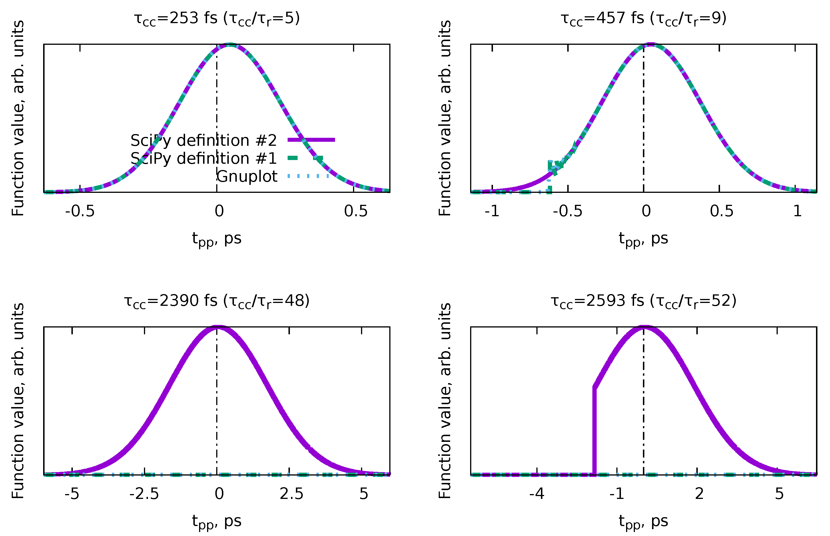
Appendix D. Issues with Numerical Implementation of the Bt(tpp) Basis Function

The B t ( t pp ) basis function (Equation (80)), and also the B to ( t pp ) basis function (Equation (83)), have issues in the numerical usage, due to the unstable behavior in the t pp < 0 region, where the near-zero ( 1 + erf ( x ) ) function is being multiplied by an exponential function, which highlights all the small numerical noise effects.
To demonstrate it, we can calculate the B t ( t pp ) with different ratios τ cc / τ r . Here, we compare three alternative numerical representations of B t ( t pp ) with τ r = 50 fs and τ r = 253 , 457 , 2390 , 2593 fs. The B t ( t pp ) was computed using the Gnuplot’s implementation of ( 1 + erf ( x ) ) , and with two alternative Python implementations of ( 1 + erf ( x ) ) from SciPy package [73]: using scipy.special.erf (definition #1) and using the cumulative distribution function of the normal distribution scipy.stats.norm.cdf (definition #2).
The results are shown in Figure A1. As one can see, at ratio τ cc / τ r = 5 , all three numerical results are equivalent. At the ratio τ cc / τ r = 9 , the Gnuplot and definition #1 start to fail, producing spurious oscillations near t pp = 0.5 ps. At higher ratios, they eventually both fail, producing zeros. The definition #2 (through cumulative distribution function) is the most stable, allowing to reach τ cc / τ r = 48 . However, at τ cc / τ r = 52 even definition #2 starts to fail, producing a cutoff at t pp = 1.8 , which is an abrupt break. Therefore, a stable ratio τ cc / τ r , where the definition #2 works stably is estimated to be τ cc / τ r < 50 .
Figure A1. Illustration of numerical calculation of the B t ( t pp ) basis function (Equation (80)) with alternative numerical functions and various ratios of τ cc / τ r . Here, τ r = 50 fs and the region plotted is 2.5 · τ cc t pp + 2.5 · τ cc .
Photochem 04 00005 g0a1

References

  1. Zewail, A.H. Femtochemistry: Atomic-Scale Dynamics of the Chemical Bond Using Ultrafast Lasers (Nobel Lecture). Angew. Chem. Int. Ed. 2000, 39, 2586–2631. [Google Scholar] [CrossRef]
  2. Young, L.; Ueda, K.; Gühr, M.; Bucksbaum, P.H.; Simon, M.; Mukamel, S.; Rohringer, N.; Prince, K.C.; Masciovecchio, C.; Meyer, M.; et al. Roadmap of ultrafast X-ray atomic and molecular physics. J. Phys. At. Mol. Opt. Phys. 2018, 51, 032003. [Google Scholar] [CrossRef]
  3. Zettergren, H.; Domaracka, A.; Schlathölter, T.; Bolognesi, P.; Díaz-Tendero, S.; Łabuda, M.; Tosic, S.; Maclot, S.; Johnsson, P.; Steber, A.; et al. Roadmap on dynamics of molecules and clusters in the gas phase. Eur. Phys. J. 2021, 75, 152. [Google Scholar] [CrossRef]
  4. Hertel, I.V.; Radloff, W. Ultrafast dynamics in isolated molecules and molecular clusters. Rep. Prog. Phys. 2006, 69, 1897. [Google Scholar] [CrossRef]
  5. Scutelnic, V.; Tsuru, S.; Pápai, M.; Yang, Z.; Epshtein, M.; Xue, T.; Haugen, E.; Kobayashi, Y.; Krylov, A.I.; Møller, K.B.; et al. X-ray transient absorption reveals the 1Au (nπ*) state of pyrazine in electronic relaxation. Nat. Commun. 2021, 12, 5003. [Google Scholar] [CrossRef]
  6. Lee, J.W.L.; Tikhonov, D.S.; Chopra, P.; Maclot, S.; Steber, A.L.; Gruet, S.; Allum, F.; Boll, R.; Cheng, X.; Düsterer, S.; et al. Time-resolved relaxation and fragmentation of polycyclic aromatic hydrocarbons investigated in the ultrafast XUV-IR regime. Nat. Commun. 2021, 12, 6107. [Google Scholar] [CrossRef] [PubMed]
  7. Garg, D.; Lee, J.W.L.; Tikhonov, D.S.; Chopra, P.; Steber, A.L.; Lemmens, A.K.; Erk, B.; Allum, F.; Boll, R.; Cheng, X.; et al. Fragmentation Dynamics of Fluorene Explored Using Ultrafast XUV-Vis Pump-Probe Spectroscopy. Front. Phys. 2022, 10, 880793. [Google Scholar] [CrossRef]
  8. Calegari, F.; Ayuso, D.; Trabattoni, A.; Belshaw, L.; Camillis, S.D.; Anumula, S.; Frassetto, F.; Poletto, L.; Palacios, A.; Decleva, P.; et al. Ultrafast electron dynamics in phenylalanine initiated by attosecond pulses. Science 2014, 346, 336–339. [Google Scholar] [CrossRef] [PubMed]
  9. Wolf, T.J.A.; Paul, A.C.; Folkestad, S.D.; Myhre, R.H.; Cryan, J.P.; Berrah, N.; Bucksbaum, P.H.; Coriani, S.; Coslovich, G.; Feifel, R.; et al. Transient resonant Auger—Meitner spectra of photoexcited thymine. Faraday Discuss. 2021, 228, 555–570. [Google Scholar] [CrossRef] [PubMed]
  10. Onvlee, J.; Trippel, S.; Küpper, J. Ultrafast light-induced dynamics in the microsolvated biomolecular indole chromophore with water. Nat. Commun. 2022, 13, 7462. [Google Scholar] [CrossRef]
  11. Malý, P.; Brixner, T. Fluorescence-Detected Pump–Probe Spectroscopy. Angew. Chem. Int. Ed. 2021, 60, 18867–18875. [Google Scholar] [CrossRef]
  12. Press, W.H.; Teukolsky, S.A.; Vetterling, W.T.; Flannery, B.P. Numerical Recipes 3rd Edition: The Art of Scientific Computing, 3rd ed.; Cambridge University Press: New York, NY, USA, 2007. [Google Scholar]
  13. Mosegaard, K.; Tarantola, A. Monte Carlo sampling of solutions to inverse problems. J. Geophys. Res. Solid Earth 1995, 100, 12431–12447. [Google Scholar] [CrossRef]
  14. Bingham, D.; Butler, T.; Estep, D. Inverse Problems for Physics-Based Process Models. Annu. Rev. Stat. Its Appl. 2024, 11. [Google Scholar] [CrossRef]
  15. Tikhonov, A.N. Solution of incorrectly formulated problems and the regularization method. Soviet Math. Dokl. 1963, 4, 1035–1038. [Google Scholar]
  16. Tikhonov, A.; Leonov, A.; Yagola, A. Nonlinear Ill-Posed Problems; Chapman & Hall: London, UK, 1998. [Google Scholar]
  17. Hoerl, A.E.; Kennard, R.W. Ridge Regression: Biased Estimation for Nonorthogonal Problems. Technometrics 1970, 12, 55–67. [Google Scholar] [CrossRef]
  18. Pedersen, S.; Zewail, A.H. Femtosecond real time probing of reactions XXII Kinetic description of probe absorption fluorescence depletion and mass spectrometry. Mol. Phys. 1996, 89, 1455–1502. [Google Scholar] [CrossRef]
  19. Hadamard, J. Sur les problèmes aux dérivés partielles et leur signification physique. Princet. Univ. Bull. 1902, 13, 49–52. [Google Scholar]
  20. Tikhonov, D.S.; Vishnevskiy, Y.V.; Rykov, A.N.; Grikina, O.E.; Khaikin, L.S. Semi-experimental equilibrium structure of pyrazinamide from gas-phase electron diffraction. How much experimental is it? J. Mol. Struct. 2017, 1132, 20–27. [Google Scholar] [CrossRef]
  21. Hestenes, M.R.; Stiefel, E. Methods of conjugate gradients for solving linear systems. J. Res. Natl. Bur. Stand. 1952, 49, 409–436. [Google Scholar] [CrossRef]
  22. Powell, M.J.D. An efficient method for finding the minimum of a function of several variables without calculating derivatives. Comput. J. 1964, 7, 155–162. [Google Scholar] [CrossRef]
  23. Tibshirani, R. Regression Shrinkage and Selection via the Lasso. J. R. Stat. Soc. Ser. (Methodol.) 1996, 58, 267–288. [Google Scholar] [CrossRef]
  24. Santosa, F.; Symes, W.W. Linear Inversion of Band-Limited Reflection Seismograms. SIAM J. Sci. Stat. Comput. 1986, 7, 1307–1330. [Google Scholar] [CrossRef]
  25. Bauer, F.; Lukas, M.A. Comparing parameter choice methods for regularization of ill-posed problems. Math. Comput. Simul. 2011, 81, 1795–1841. [Google Scholar] [CrossRef]
  26. Chiu, N.; Ewbank, J.; Askari, M.; Schäfer, L. Molecular orbital constrained gas electron diffraction studies: Part I. Internal rotation in 3-chlorobenzaldehyde. J. Mol. Struct. 1979, 54, 185–195. [Google Scholar] [CrossRef]
  27. Baše, T.; Holub, J.; Fanfrlík, J.; Hnyk, D.; Lane, P.D.; Wann, D.A.; Vishnevskiy, Y.V.; Tikhonov, D.; Reuter, C.G.; Mitzel, N.W. Icosahedral Carbaboranes with Peripheral Hydrogen—Chalcogenide Groups: Structures from Gas Electron Diffraction and Chemical Shielding in Solution. Chem.—Eur. J. 2019, 25, 2313–2321. [Google Scholar] [CrossRef]
  28. Vishnevskiy, Y.V.; Tikhonov, D.S.; Reuter, C.G.; Mitzel, N.W.; Hnyk, D.; Holub, J.; Wann, D.A.; Lane, P.D.; Berger, R.J.F.; Hayes, S.A. Influence of Antipodally Coupled Iodine and Carbon Atoms on the Cage Structure of 9,12-I2-closo-1,2-C2B10H10: An Electron Diffraction and Computational Study. Inorg. Chem. 2015, 54, 11868–11874. [Google Scholar] [CrossRef] [PubMed]
  29. Metropolis, N.; Rosenbluth, A.W.; Rosenbluth, M.N.; Teller, A.H.; Teller, E. Equation of State Calculations by Fast Computing Machines. J. Chem. Phys. 2004, 21, 1087–1092. [Google Scholar] [CrossRef]
  30. Hastings, W.K. Monte Carlo sampling methods using Markov chains and their applications. Biometrika 1970, 57, 97–109. [Google Scholar] [CrossRef]
  31. Rosenbluth, M.N. Genesis of the Monte Carlo Algorithm for Statistical Mechanics. AIP Conf. Proc. 2003, 690, 22–30. [Google Scholar] [CrossRef]
  32. Snellenburg, J.J.; Laptenok, S.; Seger, R.; Mullen, K.M.; van Stokkum, I.H.M. Glotaran: A Java-Based Graphical User Interface for the R Package TIMP. J. Stat. Softw. 2012, 49, 1–22. [Google Scholar] [CrossRef]
  33. Müller, C.; Pascher, T.; Eriksson, A.; Chabera, P.; Uhlig, J. KiMoPack: A python Package for Kinetic Modeling of the Chemical Mechanism. J. Phys. Chem. 2022, 126, 4087–4099. [Google Scholar] [CrossRef] [PubMed]
  34. Arecchi, F.; Bonifacio, R. Theory of optical maser amplifiers. IEEE J. Quantum Electron. 1965, 1, 169–178. [Google Scholar] [CrossRef]
  35. Lindh, L.; Pascher, T.; Persson, S.; Goriya, Y.; Wärnmark, K.; Uhlig, J.; Chábera, P.; Persson, P.; Yartsev, A. Multifaceted Deactivation Dynamics of Fe(II) N-Heterocyclic Carbene Photosensitizers. J. Phys. Chem. 2023, 127, 10210–10222. [Google Scholar] [CrossRef] [PubMed]
  36. Brückmann, J.; Müller, C.; Friedländer, I.; Mengele, A.K.; Peneva, K.; Dietzek-Ivanšić, B.; Rau, S. Photocatalytic Reduction of Nicotinamide Co-factor by Perylene Sensitized RhIII Complexes**. Chem.—Eur. J. 2022, 28, e202201931. [Google Scholar] [CrossRef] [PubMed]
  37. Shchatsinin, I.; Laarmann, T.; Zhavoronkov, N.; Schulz, C.P.; Hertel, I.V. Ultrafast energy redistribution in C60 fullerenes: A real time study by two-color femtosecond spectroscopy. J. Chem. Phys. 2008, 129, 204308. [Google Scholar] [CrossRef] [PubMed]
  38. Van Stokkum, I.H.; Larsen, D.S.; van Grondelle, R. Global and target analysis of time-resolved spectra. Biochim. Biophys. Acta (BBA)-Bioenerg. 2004, 1657, 82–104. [Google Scholar] [CrossRef]
  39. Connors, K. Chemical Kinetics: The Study of Reaction Rates in Solution; VCH Publishers, Inc.: New York, NY, USA, 1990. [Google Scholar]
  40. Atkins, P.; Paula, J. Atkins’ Physical Chemistry; Oxford University Press: Oxford, UK, 2008. [Google Scholar]
  41. Rivas, D.E.; Serkez, S.; Baumann, T.M.; Boll, R.; Czwalinna, M.K.; Dold, S.; de Fanis, A.; Gerasimova, N.; Grychtol, P.; Lautenschlager, B.; et al. High-temporal-resolution X-ray spectroscopy with free-electron and optical lasers. Optica 2022, 9, 429–430. [Google Scholar] [CrossRef]
  42. Debnath, T.; Mohd Yusof, M.S.B.; Low, P.J.; Loh, Z.H. Ultrafast structural rearrangement dynamics induced by the photodetachment of phenoxide in aqueous solution. Nat. Commun. 2019, 10, 2944. [Google Scholar] [CrossRef]
  43. Atkins, P.; Friedman, R. Molecular Quantum Mechanics; OUP Oxford: Oxford, UK, 2011. [Google Scholar]
  44. Manzano, D. A short introduction to the Lindblad master equation. AIP Adv. 2020, 10, 025106. [Google Scholar] [CrossRef]
  45. Tikhonov, D.S.; Blech, A.; Leibscher, M.; Greenman, L.; Schnell, M.; Koch, C.P. Pump-probe spectroscopy of chiral vibrational dynamics. Sci. Adv. 2022, 8, eade0311. [Google Scholar] [CrossRef] [PubMed]
  46. Sun, W.; Tikhonov, D.S.; Singh, H.; Steber, A.L.; Pérez, C.; Schnell, M. Inducing transient enantiomeric excess in a molecular quantum racemic mixture with microwave fields. Nat. Commun. 2023, 14, 934. [Google Scholar] [CrossRef] [PubMed]
  47. Hatano, N. Exceptional points of the Lindblad operator of a two-level system. Mol. Phys. 2019, 117, 2121–2127. [Google Scholar] [CrossRef]
  48. Schulz, S.; Grguraš, I.; Behrens, C.; Bromberger, H.; Costello, J.T.; Czwalinna, M.K.; Felber, M.; Hoffmann, M.C.; Ilchen, M.; Liu, H.Y.; et al. Femtosecond all-optical synchronization of an X-ray free-electron laser. Nat. Commun. 2015, 6, 5938. [Google Scholar] [CrossRef]
  49. Savelyev, E.; Boll, R.; Bomme, C.; Schirmel, N.; Redlin, H.; Erk, B.; Düsterer, S.; Müller, E.; Höppner, H.; Toleikis, S.; et al. Jitter-correction for IR/UV-XUV pump-probe experiments at the FLASH free-electron laser. New J. Phys. 2017, 19, 043009. [Google Scholar] [CrossRef]
  50. Schirmel, N.; Alisauskas, S.; Huülsenbusch, T.; Manschwetus, B.; Mohr, C.; Winkelmann, L.; Große-Wortmann, U.; Zheng, J.; Lang, T.; Hartl, I. Long-Term Stabilization of Temporal and Spectral Drifts of a Burst-Mode OPCPA System. In Proceedings of the Conference on Lasers and Electro-Optics, San Jose, CA, USA, 5–10 May 2019; p. STu4E.4. [Google Scholar] [CrossRef]
  51. Lambropoulos, P. Topics on Multiphoton Processes in Atoms**Work supported by a grant from the National Science Foundation No. MPS74-17553. Adv. At. Mol. Phys. 1976, 12, 87–164. [Google Scholar] [CrossRef]
  52. Kheifets, A.S. Wigner time delay in atomic photoionization. J. Phys. At. Mol. Opt. Phys. 2023, 56, 022001. [Google Scholar] [CrossRef]
  53. Virtanen, P.; Gommers, R.; Oliphant, T.E.; Haberland, M.; Reddy, T.; Cournapeau, D.; Burovski, E.; Peterson, P.; Weckesser, W.; Bright, J.; et al. SciPy 1.0: Fundamental Algorithms for Scientific Computing in Python. Nat. Methods 2020, 17, 261–272. [Google Scholar] [CrossRef]
  54. Chopra, P. Astrochemically Relevant Polycyclic Aromatic Hydrocarbons Investigated Using Ultrafast Pump-Probe Spectroscopy and Near-Edge X-ray Absorption Fine Structure Spectroscopy. Ph.D. Thesis, Christian-Albrechts-Universität zu Kiel, Kiel, Germany, 2022. [Google Scholar]
  55. Garg, D. Electronic Structure and Ultrafast Fragmentation Dynamics of Polycyclic Aromatic Hydrocarbons. Ph.D. Thesis, Universität Hamburg, Hamburg, Germany, 2023. [Google Scholar]
  56. Douguet, N.; Grum-Grzhimailo, A.N.; Bartschat, K. Above-threshold ionization in neon produced by combining optical and bichromatic XUV femtosecond laser pulses. Phys. Rev. A 2017, 95, 013407. [Google Scholar] [CrossRef]
  57. Strüder, L.; Epp, S.; Rolles, D.; Hartmann, R.; Holl, P.; Lutz, G.; Soltau, H.; Eckart, R.; Reich, C.; Heinzinger, K.; et al. Large-format, high-speed, X-ray pnCCDs combined with electron and ion imaging spectrometers in a multipurpose chamber for experiments at 4th generation light sources. Nucl. Instruments Methods Phys. Res. Sect. Accel. Spectrom. Detect. Assoc. Equip. 2010, 614, 483–496. [Google Scholar] [CrossRef]
  58. Erk, B.; Müller, J.P.; Bomme, C.; Boll, R.; Brenner, G.; Chapman, H.N.; Correa, J.; Düsterer, S.; Dziarzhytski, S.; Eisebitt, S.; et al. CAMP@FLASH: An end-station for imaging, electron- and ion-spectroscopy, and pump–probe experiments at the FLASH free-electron laser. J. Synchrotron. Radiat. 2018, 25, 1529–1540. [Google Scholar] [CrossRef]
  59. Rossbach, J. FLASH: The First Superconducting X-ray Free-Electron Laser. In Synchrotron Light Sources and Free-Electron Lasers: Accelerator Physics, Instrumentation and Science Applications; Jaeschke, E., Khan, S., Schneider, J.R., Hastings, J.B., Eds.; Springer International Publishing: Cham, Switzerland, 2014; pp. 1–22. [Google Scholar] [CrossRef]
  60. Beye, M.; Gühr, M.; Hartl, I.; Plönjes, E.; Schaper, L.; Schreiber, S.; Tiedtke, K.; Treusch, R. FLASH and the FLASH2020+ project—Current status and upgrades for the free-electron laser in Hamburg at DESY. Eur. Phys. J. Plus 2023, 138, 193. [Google Scholar] [CrossRef]
  61. Garcia, J.D.; Mack, J.E. Energy Level and Line Tables for One-Electron Atomic Spectra*. J. Opt. Soc. Am. 1965, 55, 654–685. [Google Scholar] [CrossRef]
  62. Martin, W.C. Improved 40ex0exi 1snl ionization energy, energy levels, and Lamb shifts for 1sns and 1snp terms. Phys. Rev. A 1987, 36, 3575–3589. [Google Scholar] [CrossRef] [PubMed]
  63. Williams, T.; Kelley, C. Gnuplot 5.4: An Interactive Plotting Program. 2021. Available online: http://www.gnuplot.info (accessed on 20 January 2020).
  64. LEVENBERG, K. A Method for the Solution of Certain Non-Linear Problems in Least Squares. Q. Appl. Math. 1944, 2, 164–168. [Google Scholar] [CrossRef]
  65. Marquardt, D.W. An Algorithm for Least-Squares Estimation of Nonlinear Parameters. J. Soc. Ind. Appl. Math. 1963, 11, 431–441. [Google Scholar] [CrossRef]
  66. Akaike, H. A new look at the statistical model identification. IEEE Trans. Autom. Control 1974, 19, 716–723. [Google Scholar] [CrossRef]
  67. Vaníček, P. Approximate spectral analysis by least-squares fit. Astrophys. Space Sci. 1969, 4, 387–391. [Google Scholar] [CrossRef]
  68. Tikhonov, D.S. Regularized weighted sine least-squares spectral analysis for gas electron diffraction data. J. Chem. Phys. 2023, 159, 174101. [Google Scholar] [CrossRef] [PubMed]
  69. Ippen, E.P.; Shank, C.V. Techniques for Measurement. In Ultrashort Light Pulses: Picosecond Techniques and Applications; Shapiro, S.L., Ed.; Springer: Berlin/Heidelberg, Germany, 1977; pp. 83–122. [Google Scholar] [CrossRef]
  70. Vardeny, Z.; Tauc, J. Picosecond coherence coupling in the pump and probe technique. Opt. Commun. 1981, 39, 396–400. [Google Scholar] [CrossRef]
  71. Lebedev, M.V.; Misochko, O.V.; Dekorsy, T.; Georgiev, N. On the nature of “coherent artifact”. J. Exp. Theor. Phys. 2005, 100, 272–282. [Google Scholar] [CrossRef]
  72. Rhodes, M.; Steinmeyer, G.; Ratner, J.; Trebino, R. Pulse-shape instabilities and their measurement. Laser Photonics Rev. 2013, 7, 557–565. [Google Scholar] [CrossRef]
  73. SciPy: Open Source Scientific Tools for Python. Available online: http://www.scipy.org/ (accessed on 18 January 2024).
  74. Van Stokkum, I.H.M.; Weißenborn, J.; Weigand, S.; Snellenburg, J.J. Pyglotaran: A lego-like Python framework for global and target analysis of time-resolved spectra. Photochem. Photobiol. Sci. 2023, 22, 2413–2431. [Google Scholar] [CrossRef]
  75. Müller, M.G.; Niklas, J.; Lubitz, W.; Holzwarth, A.R. Ultrafast Transient Absorption Studies on Photosystem I Reaction Centers from Chlamydomonas reinhardtii. 1. A New Interpretation of the Energy Trapping and Early Electron Transfer Steps in Photosystem I. Biophys. J. 2003, 85, 3899–3922. [Google Scholar] [CrossRef]
  76. Croce, R.; Müller, M.G.; Bassi, R.; Holzwarth, A.R. Carotenoid-to-Chlorophyll Energy Transfer in Recombinant Major Light-Harvesting Complex (LHCII) of Higher Plants. I. Femtosecond Transient Absorption Measurements. Biophys. J. 2001, 80, 901–915. [Google Scholar] [CrossRef]
  77. Holzwarth, A.R.; Müller, M.G.; Niklas, J.; Lubitz, W. Ultrafast Transient Absorption Studies on Photosystem I Reaction Centers from Chlamydomonas reinhardtii. 2: Mutations near the P700 Reaction Center Chlorophylls Provide New Insight into the Nature of the Primary Electron Donor. Biophys. J. 2006, 90, 552–565. [Google Scholar] [CrossRef] [PubMed]
  78. Zurek, W.H. Decoherence and the Transition from Quantum to Classical. Phys. Today 1991, 44, 36–44. [Google Scholar] [CrossRef]
  79. Zurek, W.H. Decoherence and the Transition from Quantum to Classical–Revisited. Los Alamos Sci. 2002, 27, 86–109. [Google Scholar]
Figure 1. A schematic illustration of the ill-posed LSQ problem. The bottom plot illustrates a LSQ function Φ ( P ) (solid curve) with multiple local minima (#1, #2, and #3). The circles illustrate different initial sets of parameters ( P ini ) that converge to different solutions ( P 1 , P 2 , P 3 ), shown with stars. The dashed parabolas in each of the minima represent a local approximation of the nonlinear LSQ function (Equation (6)) with a Taylor expansion up to the second order (see Equation (10)). The top plot shows the corresponding probability distributions p ( P ) exp ( Φ ( P ) ) . The three Gaussian functions represent the approximations of the localized solutions (Equation (10)) with standard deviations σ 1 , σ 2 , and σ 3 . The solid curve in the back represents an actual multivariate probability distribution according to Equation (5).
Photochem 04 00005 g001
Figure 2. A schematic illustration of the effect of regularization on the ill-posed LSQ problem. The unregularized case on the left shows a pure unregularized LSQ function ( Φ ( P ) ) with two equivalent solutions. The three regularized cases on the right show plots of the regularization function Φ reg ( P ) (bottom plots) and total function, as a sum of the Φ ( P ) + Φ reg ( P ) (top), as functions of parameter values ( P ).
Photochem 04 00005 g002
Figure 4. Three examples of pump–probe dynamics reaction schemes, extending the basic ones given in Equations (22), (25) and (27): (a) reaction scheme with multiple outcomes from the same intermediate metastable state; (b) pump–probe scheme with sequential decay of the intermediate states; (c) example of processes with multiple independent intermediate states that lead to the formation of independent and same observables. Solutions for schemes (a)–(c) are given in Appendix A.5, Appendix A.6 and Appendix A.7.
Photochem 04 00005 g004
Figure 6. A schematic representation of PP(MC ) 3 Fitting workflow.
Photochem 04 00005 g006
Figure 7. Experimental XUV-IR pump–probe photoelectron spectrum of helium, obtained in beamtime F-20191568. The horizontal dashed lines show the expected position of the photoelectron main line (at 16.2 eV) and sidebands. The experimental photoelectron maxima for higher-order sidebands are offset due to imperfection of the radius-to-energy conversion. Details are provided in the text.
Photochem 04 00005 g007
Figure 8. Photoelectron yields at the sidebands of various order and of the main line, corresponding to helium ionization (Reaction (94)), and their fits with the model from Equation (95). The points shown here were obtained as horizontal slices from Figure 7.
Photochem 04 00005 g008
Figure 9. Experimental ion yield of the fluorene dication C 13 H 10 2 + in the XUV-IR pump–probe experiment. Three plots show three independent fits of the same experimental data by the same model, given in Equation (96). Fits #1 and #2 are the results of standard fitting using Gnuplot [63], while the PP(MC ) 3 Fitting result was obtained using the software procedure from Section 4.4 using PP(MC ) 3 Fitting software. The solid vertical line indicates the t 0 from He sidebands, while the dotted vertical lines are the results of the corresponding fit result.
Photochem 04 00005 g009
Figure 10. Distributions of the nonlinear parameters of the model for the fluorene dication ion yield (Equation (96)) from the MC sampling procedure. The dashed vertical lines illustrate the values from Fit #1 and Fit #2 (violet and red, respectively, see Table 2). The vertical solid line for t 0 shows the result from the He sidebands measurements.
Photochem 04 00005 g010
Figure 11. Experimentaland fitted ion yield of the indole-water monocation. Experimental data were taken from Ref. [10]. Colored areas indicate the MC uncertainty of a corresponding component of the fit. The model is given in Equation (97).
Photochem 04 00005 g011
Figure 12. Spectrum of the indole-water monocation ion yield residuals from the fit given in Figure 11. The “intensity” is the absolute value of the rwLSSA spectral intensities obtained from the fit residuals, and the corresponding phase is shown with the point’s color.
Photochem 04 00005 g012
Figure 13. Indole -water monocation ion yield fit residuals, the maximal intensity component from the rwLSSA spectrum (Figure 12) and the fit result of the residual according to Equation (98).
Photochem 04 00005 g013
Figure 14. Examples of generated pump–probe datasets and their fits with PP(MC ) 3 Fitting. The “initial function” is the original function, and the “dataset” is the generated dataset with the given SN level. The shown datasets were generated using Equation (80) with τ cc = 335 fs and τ r = 50 fs parameters.
Photochem 04 00005 g014
Figure 15. Results of fitting the various datasets with unregularized and regularized procedures. The dotted lines represent the actual defined parameters of the dataset. SN denotes the signal-to-noise ratio for the fitted dataset.
Photochem 04 00005 g015
Table 1. Final values of the nonlinear parameters for fitting the He photoelectron main line and sidebands. Fitted curves are shown in Figure 8.
ParameterValue, fs
GlobalFit #0Fit #1Fit #2Fit #3Fit #4
t 0 + 38.5 ps 22 ± 1 22 ± 3 35 ± 4 23 ± 2 20 ± 2 15 ± 2
τ cc ( 0 ) 97 ± 3 97 ± 3
τ cc ( 1 ) 138 ± 5 143 ± 6
τ cc ( 2 ) 88 ± 2 88 ± 3
τ cc ( 3 ) 63 ± 3 62 ± 3
τ cc ( 4 ) 62 ± 7 61 ± 7
Table 2. Nonlinear parameters of the model for the fluorene dication ion yield (Equation (96)) obtained with different fit models. “Ini.” and “Fin.” denote the initial and final values according to the Marquardt–Levenberg algorithm [64,65]. All values are given in fs.
ParameterFit #1Fit #2 PP(MC ) 3 Fitting
Ini.Fin.Ini.Fin.
t 0 12.650 ps0 41 ± 3441 0 2 ± 33 11 ± 20
τ cc 97 80 ± 1018 97 104 ± 21 101 ± 10
τ r + 50 88 ± 7 150 130 ± 30 133 ± 37
τ r 50 36 ± 58 150 21 ± 40 22 ± 20
Disclaimer/Publisher’s Note: The statements, opinions and data contained in all publications are solely those of the individual author(s) and contributor(s) and not of MDPI and/or the editor(s). MDPI and/or the editor(s) disclaim responsibility for any injury to people or property resulting from any ideas, methods, instructions or products referred to in the content.

