1. Introduction
The sacroiliac (SI) joint connects the spine to the pelvis. SI dysfunction can lead to debilitating pain and significantly impact a patient’s quality of life [
1]. SI dysfunction can be caused by degeneration, inflammation, trauma, pregnancy, lumbar fusions, or hypermobility syndromes. Surgical intervention can be considered when conservative treatment, such as corticosteroid injections and physical/manual therapy, yields no sufficient response [
2]. The most common procedure for SI dysfunction involves stabilization of the SI joint, also known as minimally invasive sacroiliac joint fusion (SIJF). This results in a reduction in joint motion and thereby reduces pain. In this study three cannulated triangular titanium implants are used for SIJF (iFuse Implant System, SI-Bone, Santa Clara, CA, USA).
Despite the increasing evidence of effectiveness, some controversy exists in using interventional procedures for SIJ pain [
3]. This may be due to the fact that SI joint dysfunction can be challenging to diagnose because the symptoms can mimic those of other conditions, such as herniated discs or hip problems [
2,
4], or due to mixed results from previously used open surgery techniques [
5,
6].
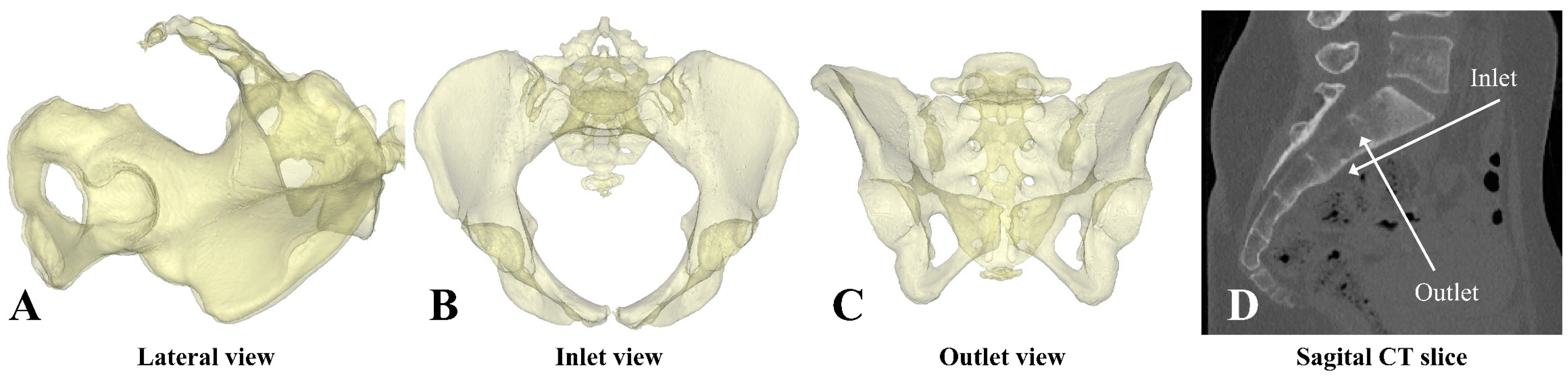
To perform a SIJF, first the surgeon predetermines the implant positions using guide pins. These pins are placed freehandedly through the SI joint using 2D lateral fluoroscopic guidance. The entry point for the guide pins is selected based on the surgeon’s experience and certain landmarks visible on a lateral fluoroscopic image. A safe trajectory needs to be confirmed in the inlet and outlet views, and the guide pins are subsequently inserted to an appropriate depth (for orientation of the pelvis in the lateral, inlet, and outlet views, see
Figure 1). Subsequently, the implants will be placed over the guide pins, and the guide pins will be removed. Placing the implants to an appropriate depth without damaging surrounding critical structures can be challenging due to the anatomical variations among patients [
7,
8,
9,
10], poor visibility on intraoperative imaging, and lack of 3D spatial information. Damaging structures, including the neural foramina, the sacral canal, or nerves (L4, L5, and obturator nerves) can result in major complications such as nerve impingement, resulting in radiating pain, numbness, or palsy [
11]. When the trajectory of an implant seems unsafe in the inlet or outlet view, the surgeon has to switch back to a lateral view and reposition the guide pin. This can be inefficient, resulting in an extended duration of surgery and increased radiation exposure. Implants sometimes loosen over time, which is another complication that can occur and result in persistent or reoccurring pain after SIJF [
3,
12]. More bone–implant contact, the use of more stable implant configurations, and the use of three implants instead of two can reduce the chance of implant loosening [
12,
13].
To overcome these challenges, navigation-guided techniques can be used [
14,
15]. These techniques supplement intraoperative imaging of the anatomy and therefore allow for optimal and safe implant positioning. However, these navigation-guided techniques are not commonly available. They are expensive and do not necessarily decrease the duration of the surgery [
16,
17]. Therefore, another more cost-effective and widely available alternative is desirable.
A suitable method may be virtual surgical planning (VSP). VSP methods are becoming widely adopted as part of standard care, as they can result in superior outcomes compared to conventional treatment without the use of VSP [
18,
19,
20,
21]. In SIJF, the lack of 3D spatial information in the intraoperative fluoroscopic images can be overcome by displaying a virtual surgical plan including 3D anatomical models and simulated fluoroscopic images, both derived from pre-operative CT data. Others have described a method using simulated fluoroscopic images to superimpose the neural foramina on fluoroscopic images [
22] and VSP without actual implants to evaluate the technical variation in SIJF due to varying sacral morphologies in cadaveric CT data [
10]. However, a combination of these techniques has never been described or introduced in clinical practice to treat SI dysfunction.
Using VSP, the implants can be virtually placed in an optimal patient-specific implant configuration that can be achieved freehandedly while avoiding critical structures. The intraoperative use of VSP may give the surgeon guidance to place the implants safely and accurately in the planned positions, which may reduce the chance of implant malpositioning and loosening [
12,
23].
This study assesses the feasibility of a developed VSP method using simulated fluoroscopic images in patients with SI dysfunction undergoing SIJF. The conformity of achieved placement to planning was retrospectively evaluated, and it was analyzed whether this improved with an increase in case numbers since there may be an initial learning curve to working with a virtual surgical plan [
24,
25,
26].
2. Materials and Methods
2.1. Study Design
We conducted a retrospective cohort study. The first ten patients who underwent a procedure after the implementation of VSP were included in this study. The workflow was implemented in November 2021 as standard clinical care for SIJF in Medisch Spectrum Twente (MST, Enschede, The Netherlands). In July 2022, the institutional review board of MST approved all clinical evaluation studies where 3D technology, including VSP, was used as standard care. All patients underwent surgery before this date and are therefore exempted from informed consent. Patient characteristics and CT imaging were taken from their electronic health records.
The developed workflow includes the use of a preoperatively created VSP based on routine pre-operative CT imaging. Some CT scans were made in other hospitals with different types of scanners and CT parameters (slice thickness ranged from 1 to 3 mm and tube voltage from 100 to 140 kVp). One experienced surgeon (approximately 100 prior SIJF surgeries) performed all interventions according to the procedure described in
Section 2.3. The surgeon could examine the 3D models, scroll through the CT scan with virtually inserted implants, and observe the simulated fluoroscopy images before and during surgery. After the intervention, a routine postoperative CT was made using the Somatom Force scanner (Siemens Healthcare, Forcheim, Germany) to verify the positioning of the implants (see
Section 2.4). In each postoperative scan, the slice thickness was 1 mm, but kVp ranged from 100 to 140 kVp. Seventy percent of the preoperative CT scans were made using the same device and settings as the postoperative CT.
2.2. Virtual Surgical Planning
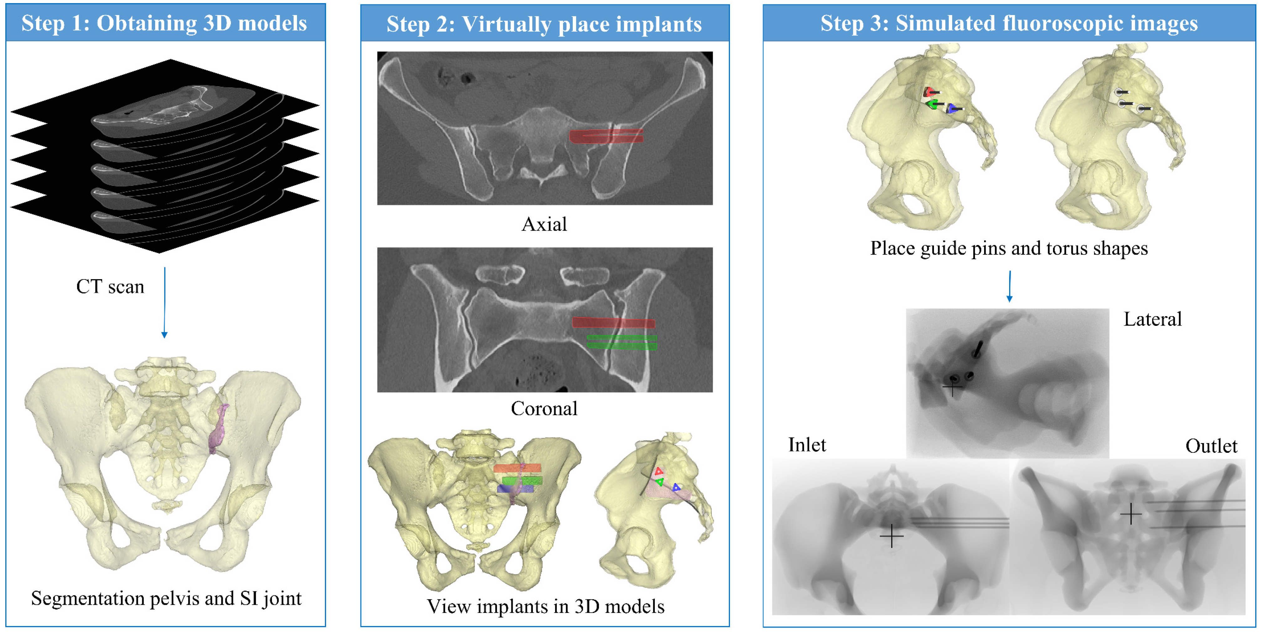
The method for VSP includes three main steps (
Figure 2). First, the 3D models of the pelvis and the SI joint were segmented based on preoperative CT imaging. Second, the implants were virtually placed inside the CT data. Third, simulated fluoroscopic images of the VSP were constructed to mimic the intraoperative fluoroscopic imaging.
Based on thresholding, the pelvis and SI joint’s synovial part were segmented from the CT scan using Mimics 23.0 (Materialise, Leuven, Belgium). The pelvis was then filled, and a 3D model was created. Filling the pelvis is necessary because the intraoperative landmarks, i.e., the ilial cortical densities (ICDs), become more visible in the lateral view when the 3D model of the pelvis is depicted transparently.
Then, the implants were virtually inserted inside the SI joint in the CT data by a technical physician. Similar to the used implant morphology, 3D models of implants ranging from 30 mm to 90 mm were constructed using 3-Matic 15.0 (Materialise, Leuven, Belgium) since no CAD files of the implants were available. Depending on the patient’s anatomy, three implants were virtually placed in the SI joint perpendicular to a true lateral view. The final position of the implants was determined based on the axial and coronal planes of the CT data. After virtually placing the implants inside the CT scan, the surgeon critically reviewed the implant positioning and confirmed the VSP.
To achieve an optimal plan for the individual patient, the number of implants, the distance between the implants, the relative position, and the implant depth are considered. Three implants were used since this gives superior outcomes compared to the use of two implants [
12,
13]. A 15 mm center-to-center distance between the parallel implants was generally maintained since this is part of the standard workflow in the used SIJF system. This distance can intraoperatively be obtained using a standard tool called the Parallel Pin Guide (iFuse Implant System). In case of unfavorable anatomy or if a different position allowed for the use of longer implants, other distances varying from 17 to 31 mm were selected. These different center-to-center distances can be achieved using the Variable Pin Guide from the system set. Using this tool, more distance between the implants will be gained, which results in more stable implant configurations [
12]. The SI joint consists of a synovial part and a ligamentous part. Approximately, the anterior one-third of the joint is the synovial part, and the posterior two-thirds is the ligamentous part [
27]. The implants are generally placed into the synovial part of the joint since this increases bone contact and, consequently, stability. Generally, the implants are virtually placed as deep as possible, but a safety margin of approximately 3 mm between the implant and the cortex of the sacrum (anterior cortex and cortex around the neural foramina) was maintained.
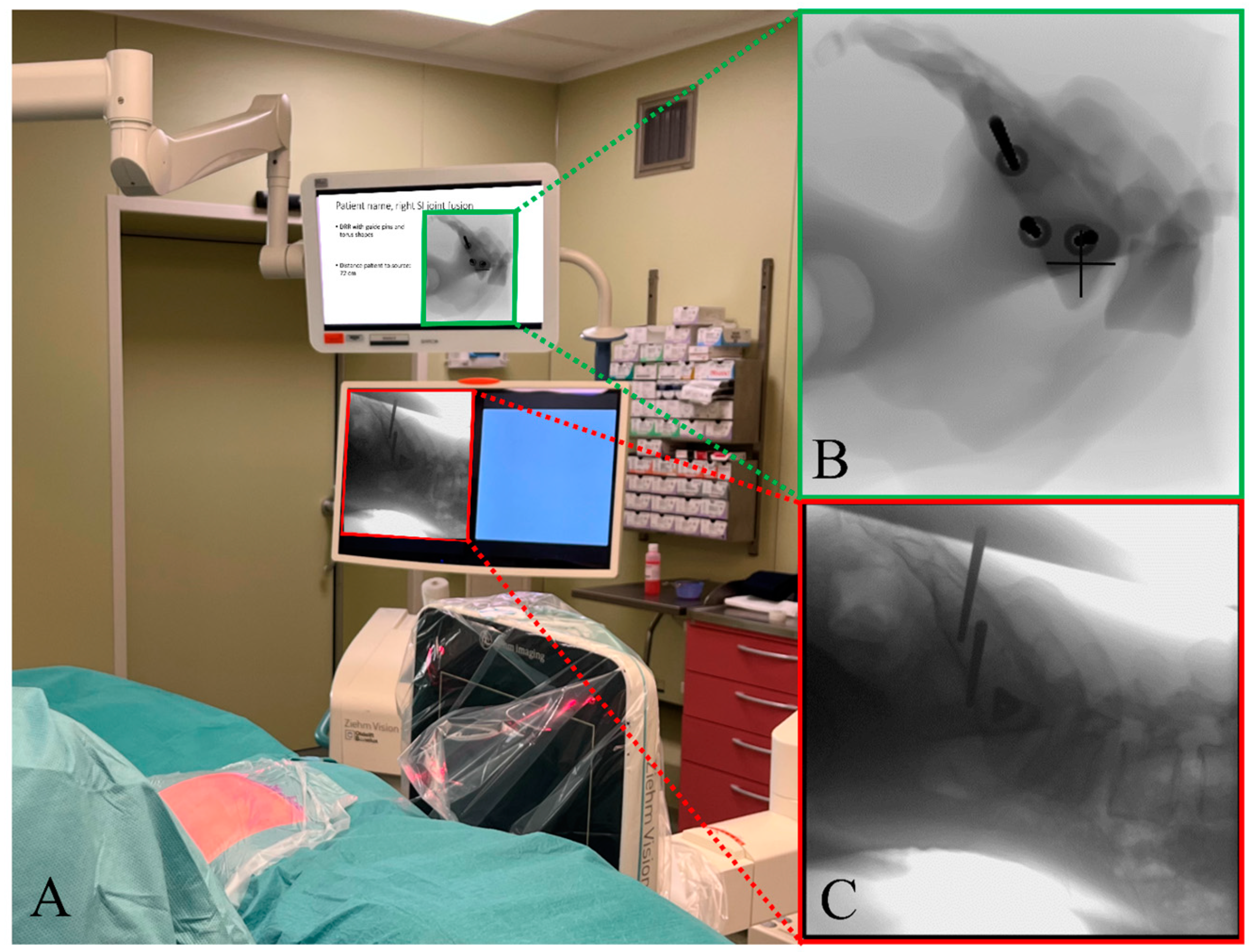
To translate the virtual surgical plan to intraoperative imaging, simulated fluoroscopic images were reconstructed. First, using 3-Matic, 3D models of the guide pins and torus shapes, which resemble the entry points in the ilium, were constructed based on the implant positions in the virtual surgical plan. Subsequently, based on the 3D models of the segmented pelvis, guide pins, and entry points, simulated fluoroscopic images were generated using the fluoroscopy module in Mimics 23.0. To make the actual and simulated fluoroscopic images as comparable as possible regarding the divergence of the X-ray beam, care was taken to equalize the position of the X-Ray source with respect to the patient (distance and center of the beam) for the actual and the simulated cases. For the simulated lateral fluoroscopic image, the distance from the virtual X-ray source to the median plane of the patient was set to 72 cm, and the position of the origin was located at an intersection point with overlapping ICDs at the height of S1. For the inlet and outlet views, the distance between the virtual X-ray source and the frontal plane was set to 72 cm. The origin was located around the sacrum. The angles of the virtual X-ray beam are determined by creating the optimal lateral, inlet and outlet views. The simulated fluoroscopic images are then added to a slideshow, along with pictures of the 3D models and a video of the CT data containing the virtually inserted implants. Therefore, the images presented comprise the following: (1) lateral view 3D model pelvis and implants; (2) inlet view 3D model pelvis and implants; (3) outlet view 3D model pelvis and implants; (4) simulated lateral fluoroscopic image; (5) simulated lateral fluoroscopic image with planned implant positions; (6) simulated lateral fluoroscopic image with planned guide pins and torus shapes; (7) simulated inlet fluoroscopic image with planned guide pins; (8) simulated inlet fluoroscopic image with planned implant positions; (9) simulated outlet fluoroscopic image with guide pins; (10) simulated outlet fluoroscopic image with implants; (11) video of CT data containing planned implant positions. This slideshow is presented on a monitor side-by-side of the fluoroscopy device during the surgery (see
Figure 3).
2.3. SIJF Procedure with VSP
First, the surgeon reproduced the simulated lateral, inlet, and outlet views using intraoperative fluoroscopic guidance, i.e., a C-arm, while the patient lies in prone position on the OR table. The simulated fluoroscopy images were displayed in a slideshow on a monitor next to the monitor of the C-arm (
Figure 3). After selecting the optimal positions for the C-arm, the position of the base of the device was locked, and the location of the lasers, incorporated in the device, were marked onto the patient. The base of the device stayed in that position, and all C-arm movements were applied to create the views (except tilting). To change between the views, the operation table was moved using a remote control instead of moving the base of the fluoroscopy device. By keeping the base in place and not tilting the device, the surgeon can more easily recreate the original views after switching between lateral, inlet, and outlet. When the views are marked onto the patient, the sterile field is created. The incision was made according to standard protocol. Then, the entry point for the first guide pin was determined using lateral fluoroscopic guidance and using the simulated lateral image (
Figure 3B) as a reference. Subsequently, using the simulated inlet and outlet views and the corresponding intraoperative fluoroscopic views, the guide pin was driven into the pelvis using a surgical hammer. Afterwards, the implant was placed over the guide pin according to standard protocol. Then, this process was repeated for the second and third implant. Using the parallel or variable pin guide, depending on the planned distance between the implants, the guide pins were placed parallel to the first. Occasionally, the surgeon deviated from the plan during surgery (for example, changing the implant length or the distance between the implants when necessary). The intraoperative fluoroscopy images consistently took precedence over the simulated fluoroscopic images.
2.4. Data Processing and Statistics
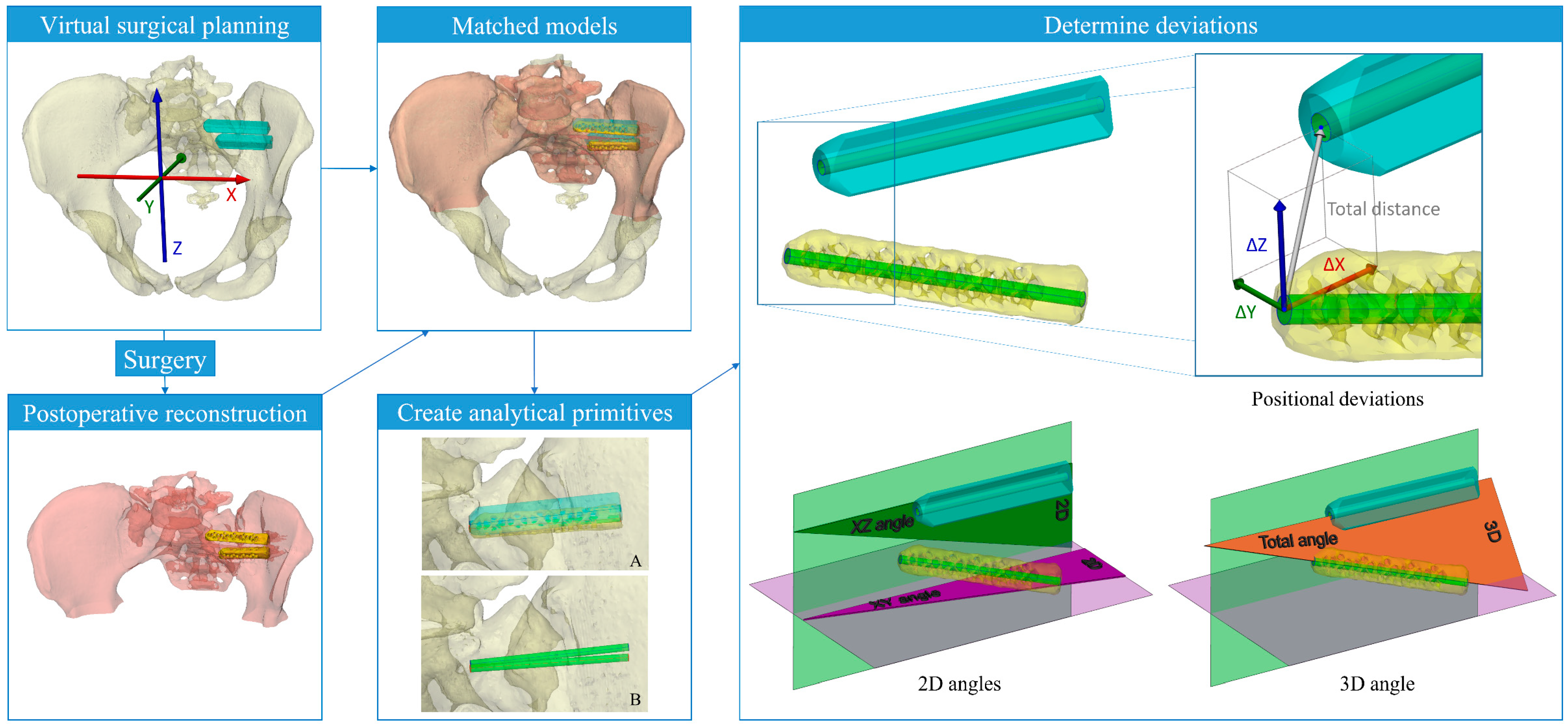
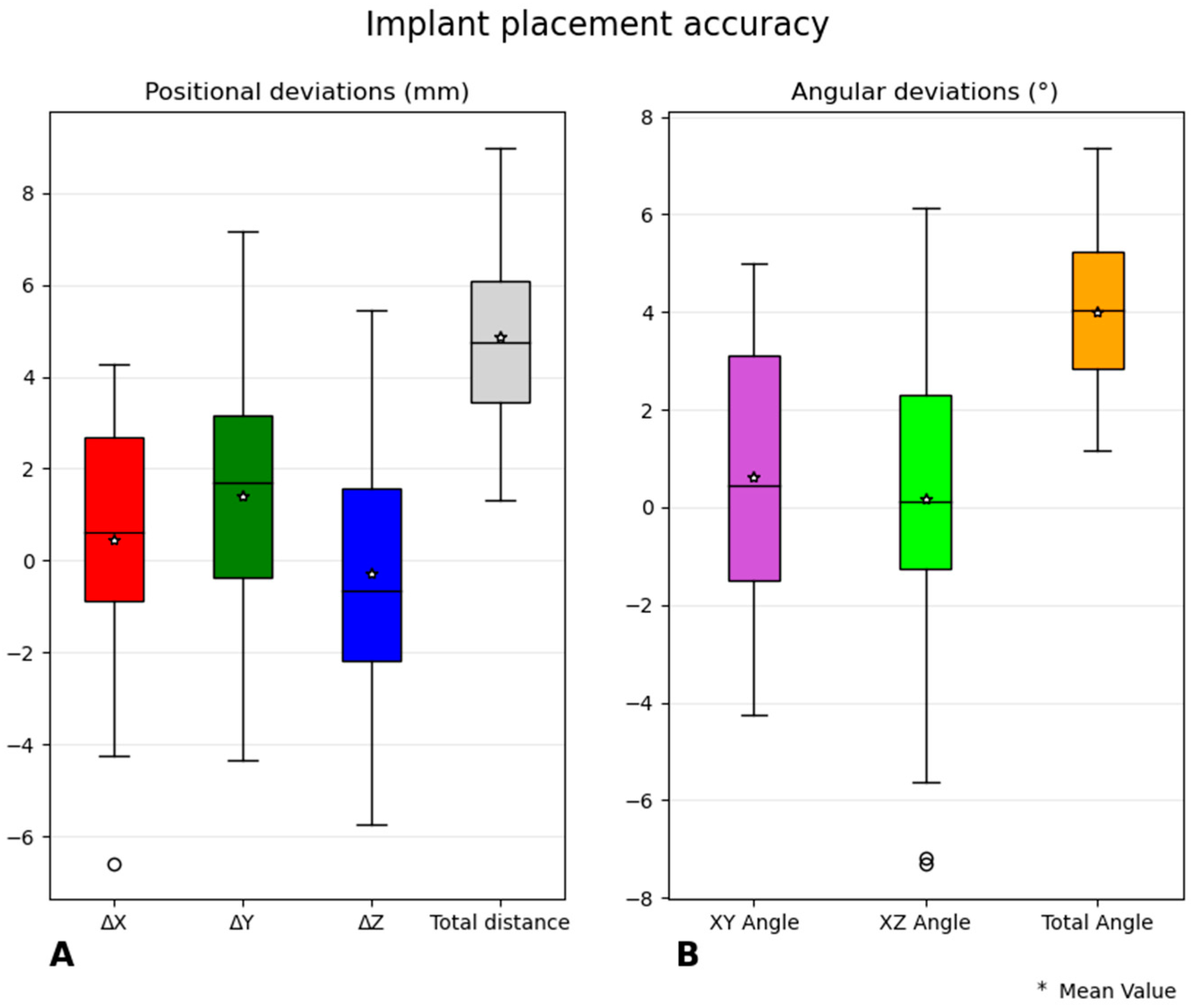
Multiple analyses were performed to evaluate the implant placement accuracy, i.e., the conformity of achieved placement, the malpositioning complications, and the possible increase in accuracy over time. To assess the implant placement accuracy, a method that compares the implant positioning in routine postoperative CT data to the implant positions in the VSP using Materialise Mimics 23.0 and 3-Matic 15.0 has been developed. The postoperative pelvis and implants were registered, i.e., matched, with the preoperative 3D model of the pelvis. Seven variables per implant were determined: four positional and three angular deviations. To derive the variables, the coordinate system of the preoperative CT was used. An overview of the method and the definition of the coordinate system is shown in
Figure 4. The positional variables are the deviation of the planned and achieved apex positions in the X, Y, and Z direction (ΔX, ΔY, and ΔZ) and the total distance between planned and postoperatively positioned apexes of the implants. The apex deviation is considered to be the best measure since this is the position where nerve damage is most likely to occur. For the angular deviations, the angle between the XY and YZ plane and the total 3D angle between the implants were determined. For convenience, the right-sided SIJF are mirrored as if they were left-sided, so outcomes of both sides can be compared. To assess the implant placement accuracy, the seven variables of all implants are presented in a boxplot. The 2D angular deviations can both be a negative or positive angle, where a negative angle indicates a clockwise rotation and a positive angle a counterclockwise rotation. Five measures (ΔX, ΔY, ΔZ, XY, and YZ angle) are relative measures. This way, when a deviation is more likely to occur in a certain direction, the mean or median deviation of a particular measure will not center around zero. This can be useful for finding flaws in the surgical method. To confirm that the mean of a deviation was different than zero, one-sample
t-tests were conducted (with
considered statistically significant). Overall, the five relative and two absolute measures express the implant placement accuracy using VSP for SIJF.
Furthermore, the number of implants penetrating the neural foramen, the sacral canal, and the anterior cortical wall of the sacrum, i.e., malpositioning complications or nerve root impingement, were monitored by analyzing the postoperative CT data.
Descriptive statistics were performed, and normality checks were performed via histogram analysis. Therefore, data are expressed as mean + standard deviation (SD) or median + interquartile range (IQR).
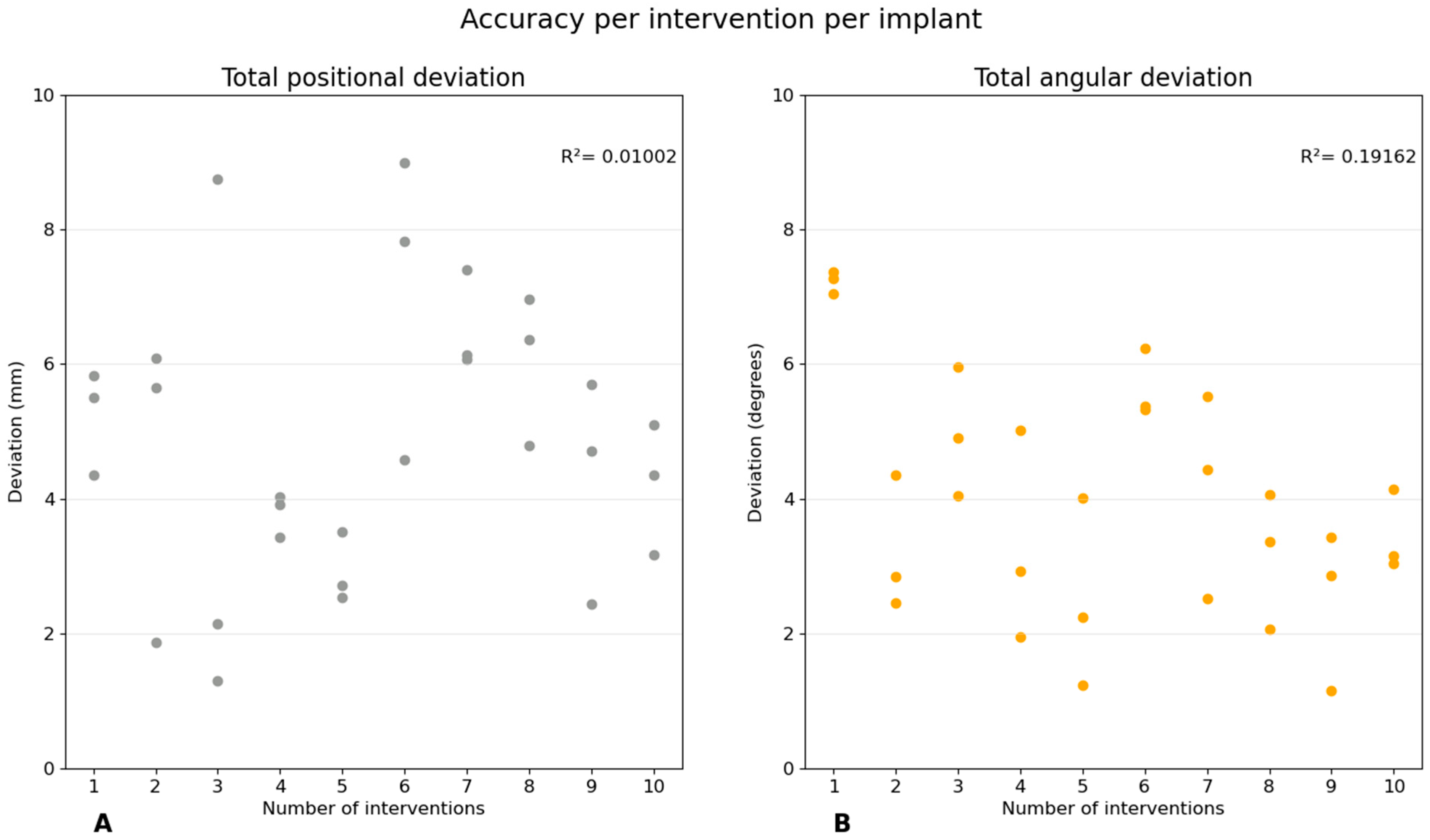
To determine whether the accuracy improved with an increase in case numbers, the total positional deviations and total angular deviations per intervention were plotted per intervention per implant. To assess whether a certain trend is present in the data when the case number increases, the coefficients of determination () were determined.
4. Discussion
This study is the first to assess the feasibility of combining VSP and simulated fluoroscopic images using a quantitative evaluation method to improve implant placement accuracy SIJF for patients suffering from SI dysfunction. The surgeon was exceptionally positive about VSP, as it helped the him understand the patient’s anatomy and determine the optimal position and length of the implants.
Studies on SIJF comparing implant placement accuracy are not yet available; yet, in spine surgery, similar analyses have been performed [
28]. Pijpker et al. evaluated the placement accuracy of pedicle and lateral mass implants using drill guides with an entry point deviation of 1.40 ± 0.81 mm and a 3D angular deviation of 6.70 ± 3.77° (mean ± standard deviation) [
28]. The results of our study cannot directly be compared to theirs, but considering the higher angular deviation, it is assumed that the deviation at the apex would be similar to our findings. Our study utilized a freehanded surgical approach, which may explain the slightly lower accuracy observed in our cases. Ultimately, similar to spine surgery, the use of patient-specific surgical guides could lead to a more accurate recreation of the virtual surgical plan during SIJF. A surgical guide for SIJF might also enable more stable, trans-articular (non-parallel) implant configurations [
23]. However, due to the minimally invasive nature of SIJF guide, seating directly on the bone is problematic. Currently, this is not possible solely using 2D fluoroscopic guidance.
The data in
Figure 4 indicate that positional deviations may occur slightly more in a particular direction. ΔX showed a trend towards the lateral direction (+ΔX), but this was not statistically significant. The ΔY values were statistically different than zero, showing a trend towards the posterior direction. The slope of the ilium can explain the +ΔY since this slope descends mostly in the posterior direction, and it is assumed that this slope can influence the positioning of the guide pins. A +ΔX (lateral direction) may be explained by the surgeon being careful enough to not place the implants too deep.
The remaining deviation observed in our study, which can be attributed to the freehanded approach, is likely the primary factor. However, an alternative explanation could be that the angle of the intraoperative lateral fluoroscopic images slightly deviates from the simulated image due to the patient being in a slightly tilted position or improper positioning of the C-arm. Furthermore, in some cases, obtaining an intraoperative true lateral view is even more challenging due to the absence of anatomical landmarks, i.e., the ICDs, on fluoroscopic imaging. Not obtaining a true lateral view likely ranks as the second most significant contributor to the remaining deviation in implant placement accuracy. Ideally, displaying the VSP onto the intraoperative images would be even more helpful, also for the inlet and outlet views. Therefore, a method that is able to superimpose the virtual surgical plan onto intraoperative fluoroscopic images should be developed [
22]. This can replace the simulated fluoroscopic images and would likely increase the implant placement accuracy.
In ten SIJFs, thirty implants were placed without major complications, such as nerve root impingement; therefore, no revision was required to retract an implant. Since we observed a relatively high accuracy and the fact that no malpositioning complications occurred, VSP for SIJF seemingly has a clinically acceptable level of accuracy.
In a study by Duhon et al., 3 out of 172 patients developed neuropathic pain related to nerve impingement [
29]. Furthermore, a review by Heiney et al. described that 2.1% of the interventions required a revision due to nerve root impingement [
30]. Both of these studies indicate that this serious complications remain prevalent. Presumably, due to the use of VSP, the chance of these major complications can be reduced since the surgeon knows the anatomy of each patient and where to place the implants safely. However, to be able to draw firm conclusions on this, more surgeries using VSP should be performed. Ideally, this should be confirmed by comparing the outcomes of SIJF with VSP to the current gold standard (conventional SIJF using 2D fluoroscopic imaging).
In contrast to other new technologies implemented in clinical practice [
24,
25,
26], it seems that VSP for SIJF showed no increase in accuracy when the surgeon gained more experience in using VSP. Despite the increasing accuracy after the first five cases, the scatterplot for all ten cases seems rather random. There are three possible explanations for the absence of this increase in accuracy. First, the supplemented information is self-explanatory, and given the experience of the surgeon in reaching the targeted position, little learning is expected to be required. Rather, we expect the major gain to be in better implant positioning due to the better (virtual) planning. However, this was not part of the current study. Second, as described earlier, obtaining a true lateral view can be difficult. Therefore, a slight discrepancy of a few degrees between the fluoroscopic true lateral and the intraoperative lateral view can result in lower implant placement accuracy. This may occur randomly and may explain the apparent randomness of the scatterplot in
Figure 6. Third, in this study, the surgeon was asked to review the virtual surgical plan, and if needed, adaptations were made according to the wishes of the surgeon. This way, the surgeon was closely involved in determining the optimal position for the implants, resulting in adherence to the pre-operative plan. This also probably increased the surgeon’s trust in VSP. This trust may have resulted in the surgeon feeling confident using VSP and may have reduced the likelihood of an increase in accuracy when the surgeon became more proficient in using VSP. On the other hand, it could be that the accuracy will improve with more interventions.
A limitation of this study is that some of the preoperative CT scans were using with different CT devices and parameters. However, these different CT parameters did not seem to influence the creation of the VSP nor the registration substantially. It is preferable to have a 1 mm slice thickness and not use a high pass filter kernel for the efficient segmentation of the pelvis. Additionally, to create realistic simulated fluoroscopy images it is preferred to scw2an the pelvis completely.
A minor limitation of the quantitative evaluation method is that the coordinates of the CT data were used, and no correction was applied for patients that were slightly tilted in the CT scan. Consequently, patients’ pelvises may be slightly rotated in the coordinate system of the CT data, leading to differently orientated small directional deviations, i.e., ΔX, ΔY, ΔZ, XY angle, and XZ angle, with respect to the anatomical axes. This error is mainly present in deviations for ΔX and ΔY since this is the plane in which the patients are mostly tilted. This error does not affect the size of the deviation, and it solely affects the direction.
It is worth noting that the surgeon who performed the ten SIJF with VSP does not want to perform the surgery without VSP anymore since he believes that VSP substantially decreases the risk of implant malpositioning. From an ethical point of view, this makes it difficult to plead for a future randomized controlled trial (RCT). However, to objectively assess the added value of VSP for SIJF, a comparative study involving clinical outcomes, including the assessment of radiation dose, implant lengths, duration of the surgery, complications (malposition complications, implant loosening, wound infection, etc.), and PROMs, preferably performed by multiple surgeons, should be performed. Nevertheless, in the absence of these outcome data, this study already gives a first impression of the feasibility of VSP in SIJF.

 ,
, 


