Definition of a Global Coordinate System in the Foot for the Surgical Planning of Forefoot Corrections

Abstract

Forefoot osteotomies to improve the alignment are difficult procedures and can lead to a variety of complications. Preoperative planning in three dimensions might assist in the successful management of forefoot deformities. The purpose of this study was to develop a global coordinate system in the foot for the planning of forefoot corrections. Two strategies (CS1 and CS2) were developed for defining a global coordinate system that meets the criteria of being well-defined, robust, highly repeatable, clinically relevant, compatible with foot CT scans, independent of the ankle joint angle, and does not include bones in the forefoot. The absolute angle of rotation was used to quantify repeatability. The anatomical planes of the coordinate systems were visually inspected by an orthopedic surgeon to evaluate the clinical relevancy. The repeatability of CS1 ranged from 0.48° to 5.86°. The definition of CS2 was fully automated and, therefore, had a perfect repeatability (0°). Clinically relevant anatomical planes were observed with CS2. In conclusion, this study presents an automated method for defining a global coordinate system in the foot according to predefined requirements for the planning of forefoot corrections.

1. Introduction

Surgical reconstruction of forefoot deformities is the most common and frequently challenging pathologic condition that a foot and ankle surgeon treats [1]. In particular, forefoot corrective osteotomies to improve the alignment are difficult procedures and can lead to a variety of complications (i.e., metatarsalgia, recurrence of the deformity, and nonunion) [2,3,4]. Hallux valgus can typically be diagnosed through physical examination and standard weight-bearing lateral and anteroposterior (AP) radiographic two-dimensional (2D) images of the foot [5]. However, due to the rotational, multiplanar nature of hallux valgus, it is difficult to describe and quantify hallux valgus accurately and reliably on standard radiographic 2D images [6,7]. This can lead to unintentional corrections in untargeted planes during surgery [8]. Preoperative planning in three dimensions (3D) might assist in successfully managing forefoot deformities. The primary objective of 3D preoperative planning is to effectively correct the deformity, reduce postoperative morbidity, and maintain normal foot biomechanics [4,9]. Computed tomography (CT) makes it possible to quantify the absolute and relative position and orientation of the bones in the foot and contributes to advanced knowledge of the multiplanar nature of hallux valgus. This might assist with the preoperative planning of hallux valgus corrections and may overcome the errors induced by 2D analysis [10,11].

To do this adequately, it is crucial to define a relevant and robust global coordinate system in the foot for the preoperative planning of hallux valgus corrections. A general reporting standard for local coordinate systems was proposed by the International Society of Biomechanics (ISB) in 2002 [12]. The ISB standard is starting to become more widely adopted; however, a consensus method for defining a global coordinate system for the foot has not been established yet. Due to the continuing absence of a standardized method, there have been a number of studies that define their own global coordinate system in the foot (

Table 1. Overview of different studies that defined a global coordinate system in the foot, specifying the accompanying limitations.

Study	Limitations
Cappozo et al. [13]	Operator-dependent accuracy and repeatability
Green et al. [4]	Dependent on the scanned section of the fibula
Geng et al. [14]	Origin not explicitly defined
Ortolani et al. [15]	Origin not explicitly defined
Yoshioka et al. [16]	The ankle joint angle determines the location of the forefoot in the global coordinate system
Modenese et al. [17]	No definition of how axes intersect the origin

) [4,13,14,15,16,17]. These coordinate systems have several limitations that cannot be ignored. Firstly, the definitions of the axes are sensitive to operator-dependent accuracy and repeatability [10,18]. Secondly, they are dependent on the scanned section of the foot or foot posture. Thirdly, they lack an unambiguous definition of the origin or axes. Thus, the purpose of this study is to develop a new global coordinate system in the foot for the 3D planning of forefoot corrections.

2. Materials and Methods

2.1. Requirements to Define a Global Coordinate System

Specific requirements were formulated for the development of a new global coordinate system in the foot based on an expert panel brainstorming session and the limitations of the studies that have defined global coordinate systems in the foot (Table 1) [4,13,14,15,16,17]; thus, the global coordinate system in the foot should

• Be well defined. A well-defined coordinate system includes the definition of two axes and the position of the origin;
• Be robust. A robust coordinate system constructs the coordinate system consistently using the same definition, regardless of anatomical variations amongst patients (i.e., accessory ossicles);
• Be highly repeatable. A highly repeatable coordinate system implies the construction of exactly the same coordinate system within an individual foot if the protocol is repeated. This will enable the same foot orientation in the preoperative planning and independent analysis, regardless of the operator;
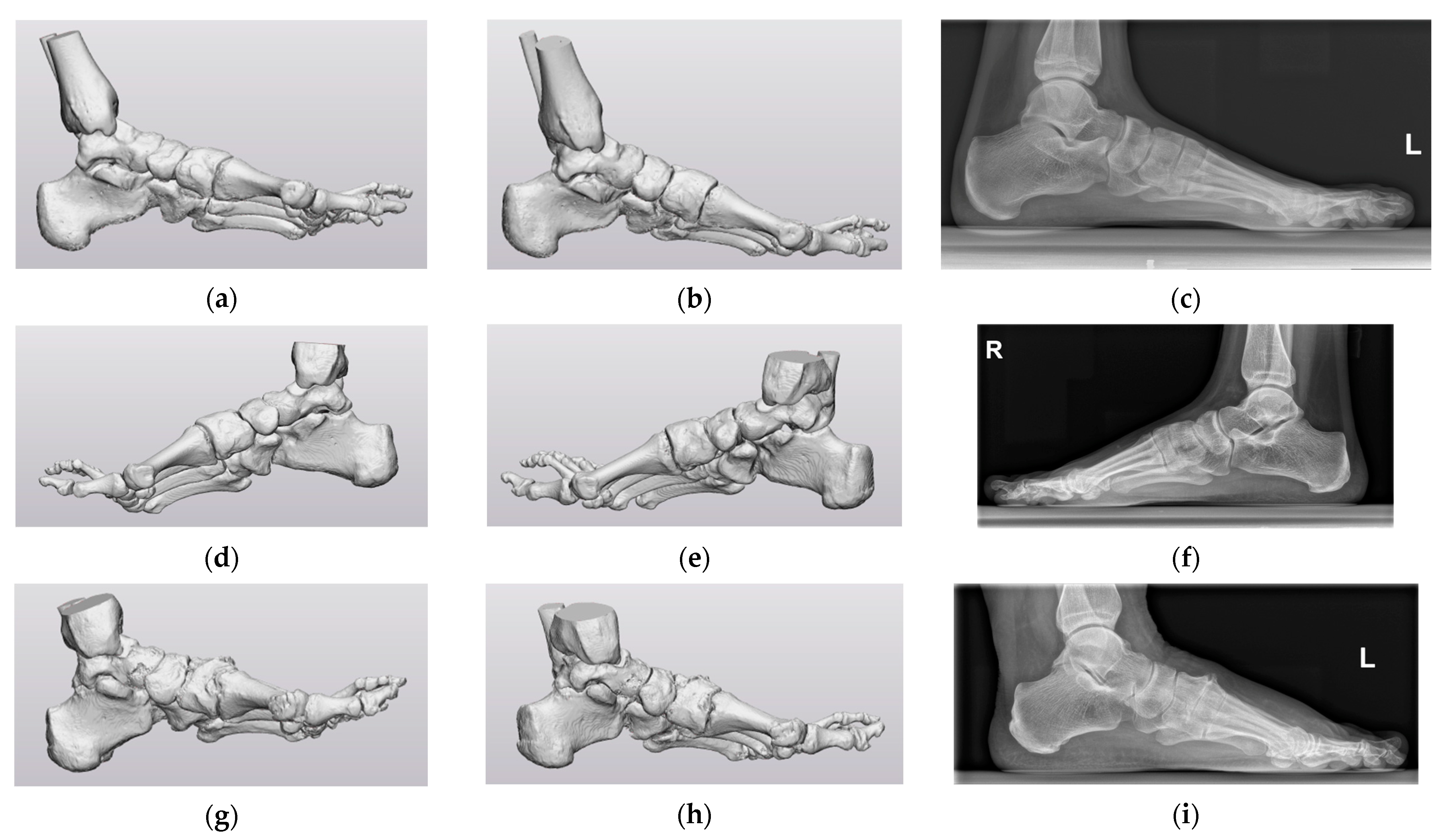
• Be clinically relevant with recognizable anatomical planes. This is necessary for the clinical interpretation of the deformity. When the virtual AP and lateral views of the coordinate system correspond with the corresponding radiographic images, a coordinate system is clinically relevant and has recognizable anatomical planes;
• Be compatible with CT scans of the foot. This will make it possible to construct the coordinate system regardless of the scanned section of the tibia and fibula;
• Not be sensitive to the ankle joint angle. This will enable the forefoot to be positioned clinically relevantly in the coordinate system, regardless of the ankle joint angle;
• Not include the shape and orientation of the bones in the forefoot by fitting an object since these bones might be deformed.

Using these requirements, two strategies were developed to define a global coordinate system in the foot. The first strategy (CS1) was to use as many points as possible on the 3D foot model (Protocol S1). The second strategy (CS2) involved applying as much automatic point selection as possible while using the points that were the furthest apart from one another (Protocol S2).

2.2. Study Design and Subjects

An observational study was conducted at the OCON Centre for Orthopedic Surgery and Sports Medicine, Hengelo, The Netherlands. Inclusion criteria for the study were patients with a hallux valgus deformity who underwent a CT scan for regular care purposes. Exclusion criteria for the study were previous hallux valgus surgery. Data were anonymized and used for the present study unless patients had opted out of use of their medical data for research purposes. A total of nine feet of nine patients (nine female), with a median age of 30 (17–63) years and a BMI of 26.2 (18.5–32.5) kg/m², were included.

2.3. Data Acquisition

CT scans were acquired on a Siemens SOMATOM Definition AS or Siemens SOMATOM Drive (Siemens Healthineers AG, Erlangen, Germany) using adjusted Materialise CT scan parameters for the foot (

Table 2. The adjusted Materialise CT scan parameters for the foot.

Helical Region of Interest	Just above the tibiotalar joint through to the carpal–metacarpal joints, dependent on the region of interest
Collimation	Slice thickness: 1.25 mm or smaller Slice increment: 0.625 mm (50% overlap)
kVp	120
mAs	As given by the automatic system
Pitch	Use 1 or smaller
Field of View (FOV)	Fit the whole foot
Matrix	Use a 512 × 512 matrix
Kernel/Algorithm	Moderate/soft tissue

), with the patient in supine position. A splint was used in six patients to create a constant plantigrade foot and neutral ankle position across patients (Figure 1). The splint prevented motion interference and provided the greatest possible replication of stance on a flat surface. The foot CT scans of the other three patients were retrospectively used without a splint.

The CT scans were exported to Materialise’s Interactive Medical Image Control System 21.0 (Mimics v21.0, Materialise NV, Leuven, Belgium) in the Digital Imaging and Communications in Medicine (DICOM) format for segmentation. A thresholding tool was used to construct a mask of all pixels with a threshold range of 226 to 3071 Hounsfield Units, and the resulting segmentation mask was then manually edited to eliminate holes. Each bone in the segmentation masks was rendered to form a 3D structure, and all bones together formed a 3D model showing the relative positions of the segmented bones in space. The Mimics program files were then converted to 3D binary formatted stereolithography (STL) files. These files were imported to 3-Matic software (Materialise NV, Leuven, Belgium) to construct the two global coordinate systems.

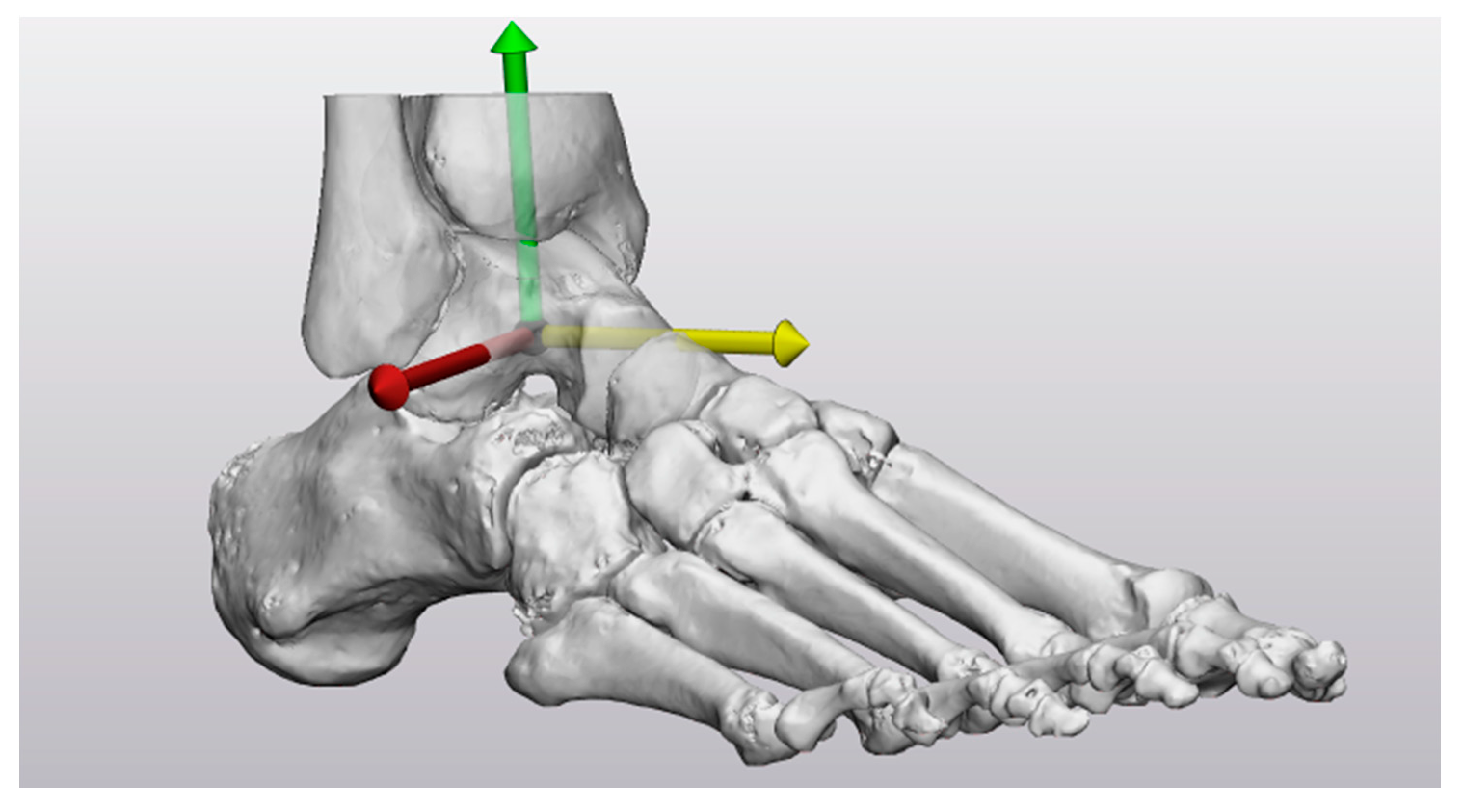
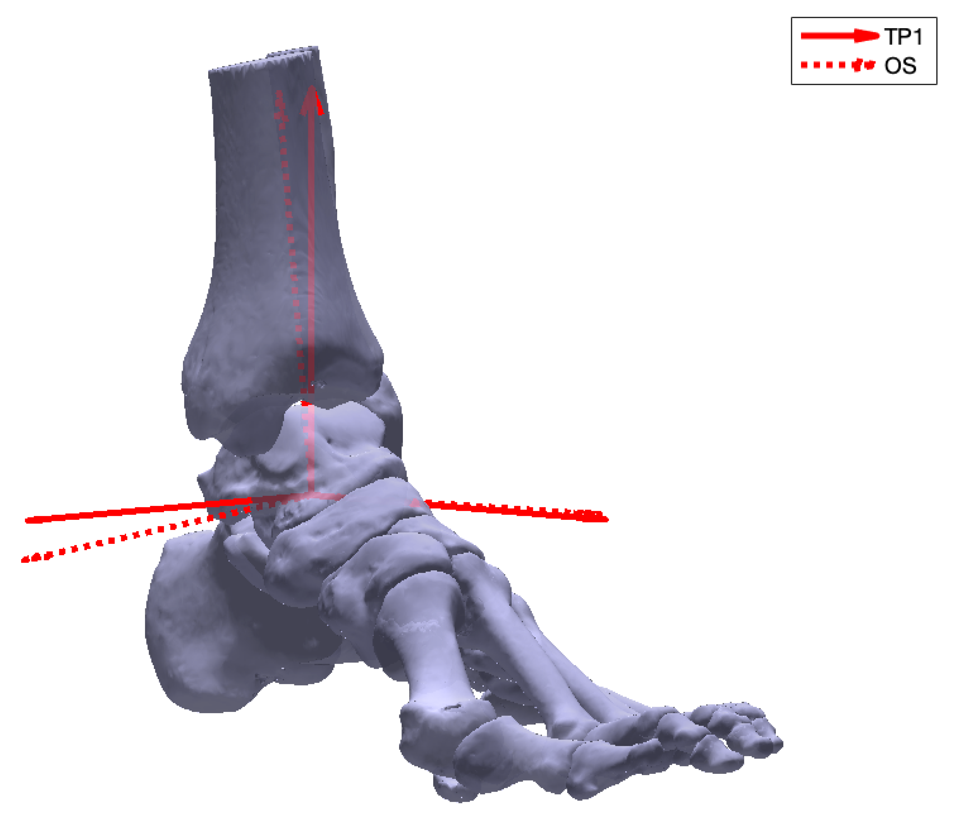
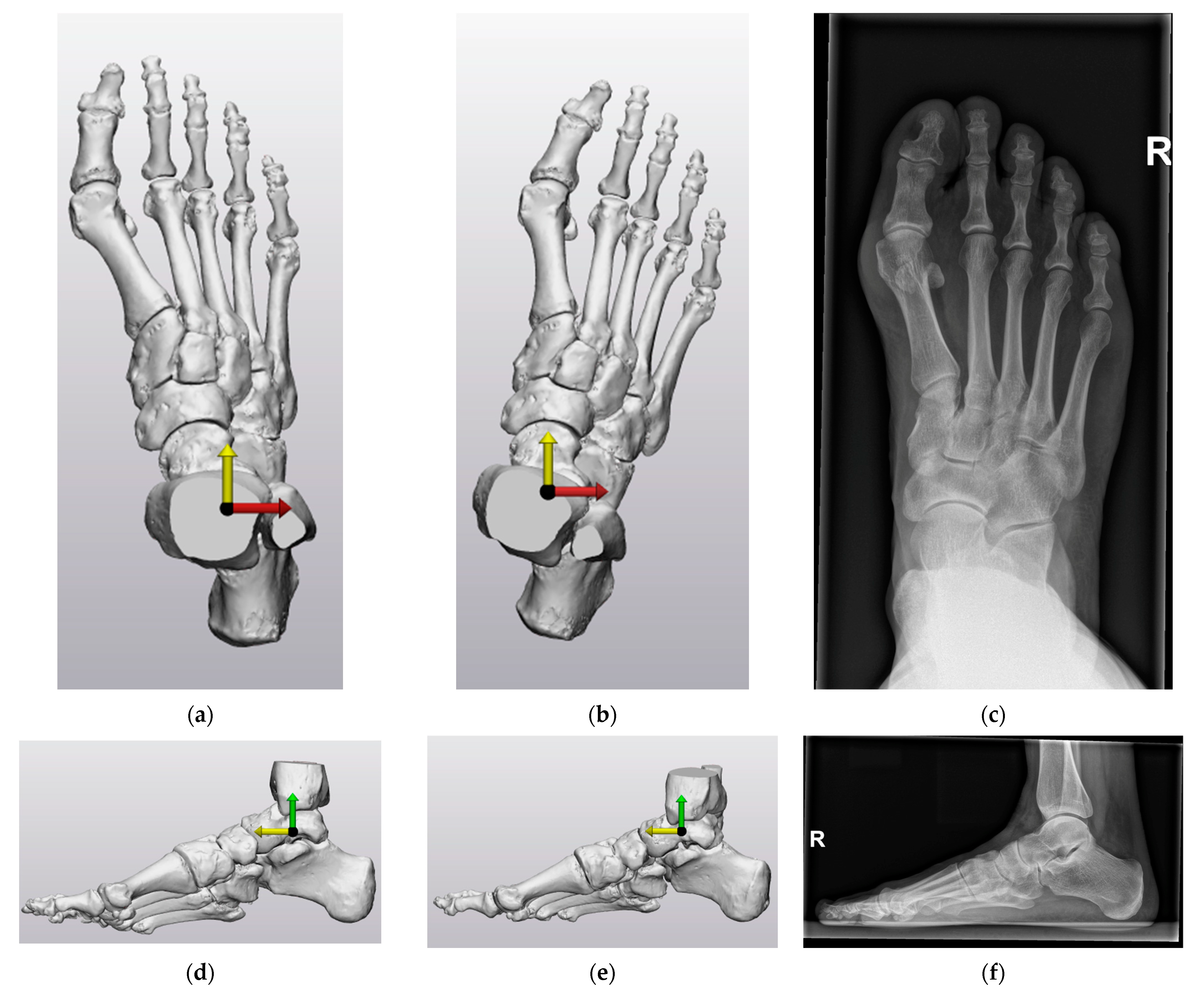
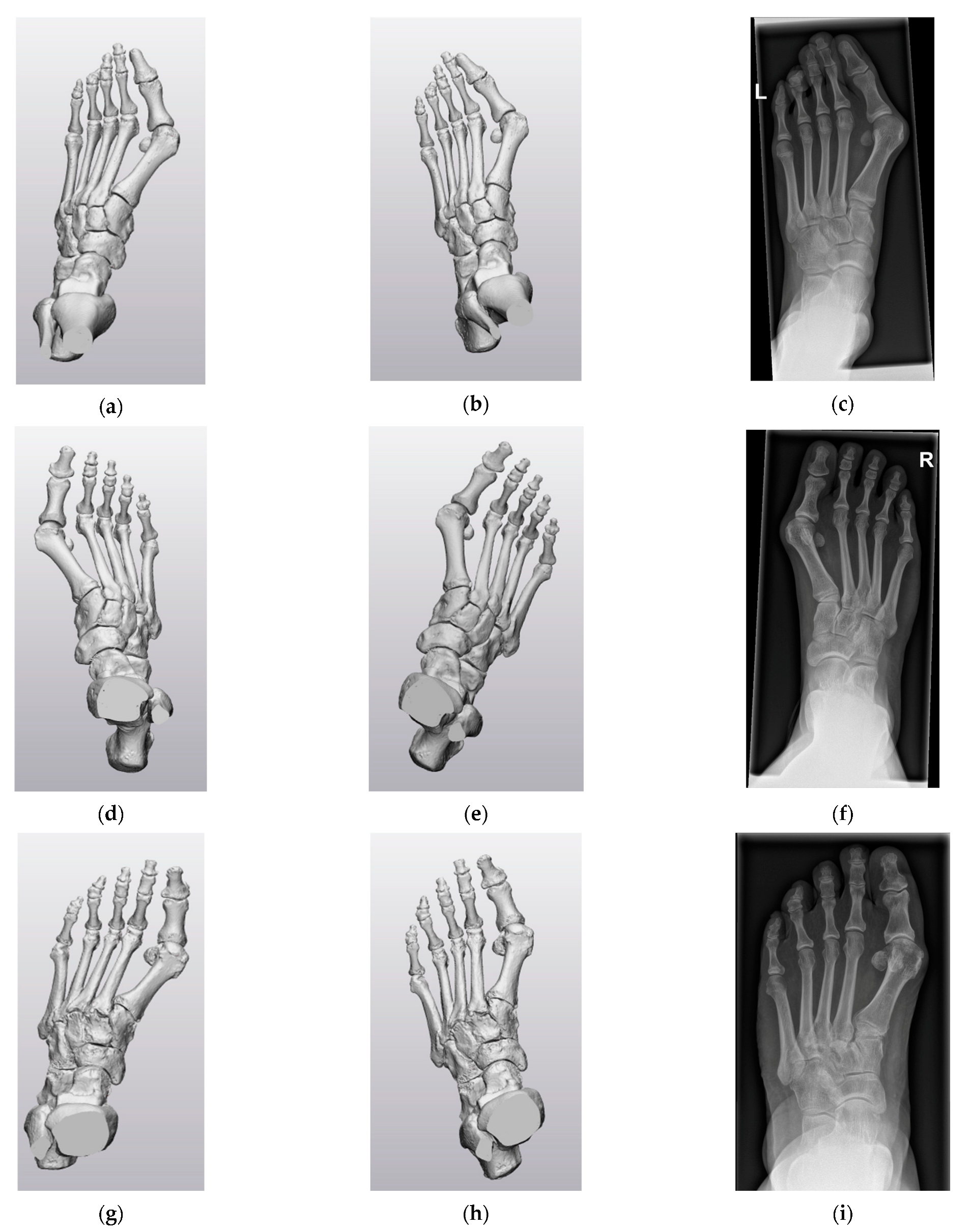
2.4. Coordinate System Definitions

This study used the direction definitions of the x- (pointing to the right), y- (pointing anteriorly), and z-axis (pointing cranially) to form axes that were clinically applicable, despite the ISB recommendations for an anteriorly pointed x-axis, a cranially pointed y-axis, and a z-axis pointed to the right [12].

The talus was used in the construction of CS1 due to its preservation throughout a broad spectrum of forefoot deformities and its availability in foot CT scans. This will develop a robust coordinate system that is compatible with CT scans of the foot, not sensitive to the ankle joint angle, and does not include bones in the forefoot. To start the construction of CS1, the facies superior of the trochlea tali was manually drawn (Figure 2a). Through this surface, a cylinder was fitted with its longitudinal axis, defining the direction of the x-axis as the normal vector to a sagittal plane (Figure 2b). The Origin (O) was defined as the midpoint of the talar intersections (TI1 and TI2) of the axis of the cylinder (Figure 2c). The y-axis was defined as follows. First, the longitudinal talus inertia axis was generated (Figure 2d), and at the intersection point with the cylinder (IPC), an additional line parallel to the x-axis was created (Figure 2e). The y-axis runs from the Origin to the intersection point of the additional line with a sagittal plane (IPS) (Figure 2f). The z-axis was orthogonal to the x-axis and y-axis (Figure 3).

The construction of CS2 was a completely automated strategy using the talus and the three weight-bearing points on the calcaneus and first and fifth metatarsal heads due to its preservation throughout a broad spectrum of forefoot deformities and availability in foot CT scans. This will develop a robust coordinate system that is compatible with CT scans of the foot, not sensitive to the ankle joint angle and does not include bone in the forefoot. To start the construction of CS2, the most caudal point of the first metatarsal–sesamoid complex (M1), fifth metatarsal (M5), and calcaneus (C) were automatically selected in the original CT scan orientation (Figure 4a). These three weight-bearing points were used to construct a ground plane (Figure 4b). The normal vector of the ground plane defined the direction of the z-axis (Figure 4c). The inertia axes of the talus were generated, with their intersection point serving as the Origin (O) (Figure 4d). To ensure an orthogonal coordinate system, the longitudinal talus inertia axis was projected on the ground plane, defining the direction of the y-axis (Figure 4e). The normal vector and the projected longitudinal talus inertia axis were translated towards the Origin to form the z-axis and y-axis (Figure 4f). The x-axis was orthogonal to the z-axis and y-axis (Figure 5).

2.5. Coordinate System Evaluation

The developed coordinate systems comply with the requirements that the global coordinate system in the foot should be well defined, be robust, be compatible with CT scans of the foot, not be sensitive to the ankle joint angle, and not include bones in the forefoot. The repeatability and clinical relevancy of the global coordinate systems in the foot were evaluated.

Evaluation of repeatability was assessed as follows. Two different operators constructed the coordinate systems of the six splinted feet independently, using different strategies. The operators were a technical physician and an orthopedic surgeon (OS). The operators were both familiar with foot anatomy and the technical physician with the employed software. The technical physician repeated the construction of each coordinate system two times for each foot with an interval of one week (TP1 and TP2). The absolute angle of rotation was used to quantify repeatability, and it describes the smallest angle of rotation between the repeated coordinate system construction of the technical physician (TP1 and TP2) and for the two operators (TP1 and OS) (Figure 6). The amount of rotation around each axis required to align two coordinate systems was depicted using the axis with angle magnitude. This was calculated for the repeated construction of the technical physician (TP1 and TP2) and for the two operators (TP1 and OS).

Evaluation of clinical relevancy was assessed by generation of virtual weight-bearing AP and lateral images for the nine 3D foot models (Figure 7). Based on the first coordinate system construction of the technical physician, the view straight at the xy-plane and yz-plane represented the virtual AP and lateral image. These virtual images represent the conventional radiographic images, which are used as a reference frame to interpret the virtual images. Orthopedic surgeons were asked if they could use the virtual images for the clinical interpretation of the deformity. The coordinate system was clinically relevant and had recognizable anatomical planes if the virtual images corresponded with the corresponding conventional radiographic images. The virtual images of the three 3D foot models without a splint allowed the assessment of the clinical relevancy without the use of a splint in the CT scan.

3. Results

CS1 intraobserver repeatability ranged from 0.48° to 2.12° (

Table 3. The absolute angle of rotation between the first (CS1) and second coordinate system (CS2) definition of the technical physician (TP1 and TP2) and between TP1 and the coordinate system definition of the orthopedic surgeon (OS).

Absolute Angle of Rotation	Patient 1	Patient 2	Patient 3	Patient 4	Patient 5	Patient 6	Mean (SD)
CS1
TP1–TP2	1.66°	0.48°	0.86°	1.48°	2.12°	1.75°	1.39° (0.61°)
TP1–OS	2.10°	1.30°	0.92°	1.35°	4.43°	5.86°	2.66° (2.01°)
CS2
TP1–TP2	0°	0°	0°	0°	0°	0°	0° (0°)
TP1–OS	0°	0°	0°	0°	0°	0°	0° (0°)

). The interobserver repeatability of CS1 ranged from 0.92° to 5.86°. CS2 was automated and, therefore, had an intra- and interobserver repeatability of 0°. More specific details on the amount of rotation around each axis necessary to align the two coordinate systems can be found in

Table 4. The axis with angle magnitude between the first (CS1) and second coordinate system (CS2) definition of the technical physician (TP1 and TP2) and between TP1 and the coordinate system definition of the orthopedic surgeon (OS).

Axis with Angle Magnitude		Patient 1	Patient 2	Patient 3	Patient 4	Patient 5	Patient 6
CS1
	x-axis	0.28°	0.10°	0.40°	1.26°	−0.56°	−0.12°
TP1–TP2	y-axis	−0.34°	−0.44°	−0.42°	0.69°	−2.00°	−1.59°
	z-axis	1.60°	−0.16°	0.63°	−0.36°	−0.46°	0.72°
	x-axis	0.50°	−1.1°	−0.40°	0.82°	0.36°	0.88°
TP1–OS	y-axis	−2.00°	−0.08°	−0.23°	0.75°	−4.03°	−5.69°
	z-axis	0.38°	−0.72°	−0.79°	0.76°	−1.81°	1.12°
CS2
	x-axis	0°	0°	0°	0°	0°	0°
TP1–TP2	y-axis	0°	0°	0°	0°	0°	0°
	z-axis	0°	0°	0°	0°	0°	0°
	x-axis	0°	0°	0°	0°	0°	0°
TP1–OS	y-axis	0°	0°	0°	0°	0°	0°
	z-axis	0°	0°	0°	0°	0°	0°

. Variation in orientation of the x-, y-, and z-axis was found for each patient in CS1. Each patient had a different axis that required the most rotation to align TP1 and TP2 or OS. For CS2, there was no deviation in orientation of the three axes between TP1 and TP2 or TP1 and OS for any of the patients.

The virtual AP and lateral images of CS1 and CS2 compared to the corresponding AP and lateral radiographic images of Patient 2 are depicted in Figure 6. Two orthopedic surgeons indicated that the virtual AP and lateral images of CS1 did not correspond to the conventional radiographic images of the foot, as the foot appears to be inclined and in endorotation. Both surgeons indicated that the virtual images of CS2 were the most recognizable and corresponded to the conventional weight-bearing AP and lateral radiographic images of the foot. However, the foot does not lay exactly straight in line in the virtual AP image of CS2. The virtual AP and lateral images of CS1 and CS2 compared to the corresponding radiographic images of the three 3D foot models without a splint are depicted in Figure A1 and Figure A2. Both orthopedic surgeons indicated that the virtual images of CS2 were the most recognizable and corresponded to the conventional weight-bearing radiographic images when not using a splint.

4. Discussion

The primary objective of this study was to establish a global coordinate system definition within the foot, specifically for the purpose of planning forefoot corrections. The study aimed to propose a well-defined, robust, and highly repeatable coordinate system that holds clinical relevance, is compatible with foot CT scans and remains independent of variations in the ankle joint angle. To achieve these objectives, the research explored and discussed two distinct strategies for defining such a global coordinate system in the foot.

The definition of CS2 was preferred because it meets all the requirements for the development of a new global coordinate system in the foot. CS2 includes the definition of two axes and the position of the origin, resulting in a well-defined coordinate system. In addition, the construction of CS2 uses the talus and three weight-bearing points of the foot due to its preservation throughout a broad spectrum of forefoot deformities and availability in foot CT scans. This creates a robust coordinate system that is constructed consistently using the same definition regardless of anatomical variations. The analysis demonstrated that the automated strategy, CS2, exhibits a high level of repeatability, both inter- and intra-operator. This repeatability is attributed to the minimal intervention required from the operator during the process of defining the coordinate system. This will enable independent analysis of each foot in the same coordinate system, regardless of the operator, as it always creates the same coordinate system. The correspondence between the virtual AP and lateral images and the weight-bearing AP and lateral radiographic images validates the clinical relevance of CS2, as it aligns with identifiable anatomical planes. Consequently, the quantification of the absolute and relative position and orientation of the foot bones can be effectively communicated in a clear and consistent manner using this coordinate system. Moreover, the construction of CS2 is completed using standard foot CT scans, and therefore, altering the parameters to extend the scanning area is not necessary. As a result, radiation exposure is not increased. Additionally, the construction of CS2 does not include bones in the forefoot and is not sensitive to the ankle joint angle, allowing the forefoot to be positioned clinically relevant in the coordinate system, regardless of the ankle joint angle. As a result, the definition of CS2 allows geometrical representations of the position and orientation of the bones in the foot for the planning of forefoot corrections.

Despite the definition of CS1 being well-defined, robust, compatible with foot CT scans, independent of the ankle joint angle, and excluding bones in the forefoot, it was not preferred because of its poor repeatability and clinical relevancy.

Although a number of previous studies proposed a global coordinate system in the foot (Table 1) [4,13,14,15,16,17], their definitions did not meet the requirements of being well-defined, robust, highly repeatable, clinically relevant, compatible with foot CT scans, independent of the ankle joint angle, and excluding bones in the forefoot. Additionally, to the best of our knowledge, this is the first study that has quantified perfect repeatability of the global coordinate system for the foot using the absolute angle of rotation. Conconi et al. previously used the absolute angle of rotation to calculate the rotational variability among local coordinate systems in the foot [10]. However, the largest rotational variability they reported was 4.2°. The current study quantified this value as poor repeatability, given its proximity to the absolute angles of rotation in the definition of CS1. In addition, this value does not match with the largest absolute angle of rotation (0°) found in the definition of CS2. This confirms the perfect repeatability found in this study. Green et al. previously referenced the x-axis and y-axis against a best-fit talar centroidal axis to evaluate the variability of the global coordinate system [4]. The calculated angles between the axes and the best-fit talar centroidal axis both had a standard deviation of 2.36°. The current study also quantified these values as poor repeatability, given its proximity to the found axis with angle magnitudes in the definition of CS1. In addition, these values do not match the largest axis with an angle magnitude (0°) found in the definition of CS2. This also confirms the perfect repeatability found in this study.

This study has several limitations. First, this study is based on only nine 3D foot models of patients with hallux valgus. This limitation is mitigated by the use of the automated method that results in perfect repeatability, but additional evaluation of the clinical relevancy may be required. Secondly, the effect of segmentation on the coordinate system is not evaluated. The inertia axes of the talus are sensitive to bone geometry for axes different from the main one (the longitudinal talus inertia axis) [10]. The bone geometry depends on how the CT scan was segmented to generate the 3D model. Different segmentation software, CT scan parameters, and operator segmentation expertise may result in differences in bone geometry. However, several studies showed high repeatability and accuracy for the segmentation process using Mimics software [19,20,21,22,23,24]. Although the exact effect of segmentation on the coordinate system is uncertain, it is believed to be negligible. Thirdly, the weight-bearing condition is not taken into account in this study. Weight-bearing CT scanners (WBCTs) enable imaging of the foot to be carried out in the natural weight-bearing position. Weight-bearing widens the forefoot when the medial ray moves through the tarsometatarsal joint [25,26,27,28]. WBCT has the advantage of reduced radiation exposure [29,30], and it improves the evaluation of forefoot deformities [14,26,27]. However, the patients in this study could not stand in the CT scanner during image acquisition. The splint (Figure 1) provided the greatest possible replication of stance on a flat surface, maintaining a constant plantigrade foot and neutral ankle position across patients. It is believed that the use of this splint results in automatically selected points on the same level as in the weight-bearing situation, leading to a similar normal vector. Consequently, weight-bearing is believed to have little to no effect on the constructed coordinate system and its virtual images. Nevertheless, it is recommended to use WBCT for the evaluation of forefoot deformities when this is available in the hospital. Fourthly, a limitation is the necessity of acquiring a CT scan for patients with minor pathologies. The availability of CT scanners can also differ from hospital to hospital or country to country. Although this is outside the scope of this study, some initiatives have been set up to transfer data from 2D radiographic images to a 3D digital model [31,32]. This might be a future solution to avoid the need for a CT scan for patients with minor pathologies. The proposed coordinate system definition of CS2 also has some limitations. First, talus deformities may result in different orientations of its inertia axes, affecting the coordinate system. In addition, talus and midfoot malalignment may lead to a different y-axis orientation relative to the forefoot. Since forefoot deformities were the focus of this study, the morphology of the hindfoot and the alignment of the talus and midfoot were assumed to be more or less normal. Secondly, the coordinate system may also be affected by the foot position in the CT scanner because of the use of the automatic point selection in the original CT scan orientation. The foot position determines the most caudal automatic selected points on the first metatarsal–sesamoid complex, fifth metatarsal, and calcaneus (Figure 4a). Consequently, plantarflexion of the ankle in the CT scanner will result in a more distal automatically selected point on the calcaneus compared to Figure 4a. However, a splint (Figure 1) solves this problem by creating a constant plantigrade foot and neutral ankle position across patients. The only factor that may have affected the automatic point selection is the skewed positioning of the patient on the table of the CT scanner. This can result in more laterally or medially selected points on the first metatarsal–sesamoid complex, fifth metatarsal, and calcaneus. However, it is believed to have little to no impact on the constructed normal vector of the ground plane. The strength of this study is that, to the best of our knowledge, this is the first study that has established and quantified the repeatability and clinical relevancy of two potential global coordinate systems in the foot.

Finally, the presented work represents the preliminary step towards preoperative 3D planning of forefoot corrections. Currently, radiographic 2D measurements are necessary for the clinical interpretation of hallux valgus (e.g., the hallux valgus angle (HVA) and intermetatarsal angle (IMA)). With the proposed coordinate system, it becomes possible to derive clinically relevant measurements from the 3D foot model by projecting them onto the virtual views of the coordinate system. For example, the longitudinal inertia axes of the first metatarsal and the proximal phalanx can be automatically generated and projected on the virtual AP view of the coordinate system to measure the HVA. Similarly, the longitudinal inertia axes of the first and second metatarsals can be automatically generated and projected on the virtual AP view of the coordinate system to measure the IMA. In future endeavors, the proposed coordinate system will be utilized to accurately identify the optimal location and appropriate procedure for correcting forefoot deformities, thus preventing the need for extensive or unplanned surgical interventions. Future research may adopt the proposed coordinate system broadly and reach a consensus in order to conduct meaningful comparisons between studies.

5. Conclusions

This study presented an automated method for defining a well-defined, robust, highly repeatable, clinically relevant, compatible with foot CT scans, independent of the ankle joint angle, and not include bones in the forefoot global coordinate system in the foot for the preoperative planning of forefoot corrections. A high repeatability is achieved by the automated method since it does not rely on manually selected landmarks or fitting spheres to the bone surfaces. Using this automated method will make it easier to quantify the absolute and relative position and orientation of the bones in the foot and contribute to advanced knowledge of foot morphology. This could provide more information on the multiplanar nature of hallux valgus, which might assist with the preoperative planning of hallux valgus corrections.

References

1. Zelen, C.M. Advances in Forefoot Surgery. Clin. Podiatr. Med. Surg. 2013, 30, 13–14. [Google Scholar] [CrossRef] [PubMed]
2. Femino, J.E.; Mueller, K. Complications of Lesser Toe Surgery. Clin. Orthop. Relat. Res. 2001, 391, 72–88. [Google Scholar] [CrossRef] [PubMed]
3. Sammarco, G.J.; Idusuyi, O.B. Complications After Surgery of the Hallux. Clin. Orthop. Relat. Res. 2001, 391, 59–71. [Google Scholar] [CrossRef] [PubMed]
4. Green, C.; Fitzpatrick, C.; FitzPatrick, D.; Stephens, M.; Quinlan, W.; Flavin, R. Definition of Coordinate System for Three-Dimensional Data Analysis in the Foot and Ankle. Foot Ankle Int. 2011, 32, 193–199. [Google Scholar] [CrossRef]
5. Kuhn, J.; Alvi, F. Hallux Valgus, StatPearls. Treasure Island (FL). Available online: https://www.ncbi.nlm.nih.gov/books/NBK553092/ (accessed on 30 June 2023).
6. Gutekunst, D.J.; Liu, L.; Ju, T.; Prior, F.W.; Sinacore, D.R. Reliability of clinically relevant 3D foot bone angles from quantitative computed tomography. J. Foot Ankle Res. 2013, 6, 38. [Google Scholar] [CrossRef]
7. Welck, M.J.; Al-Khudairi, N. Imaging of Hallux Valgus How to Approach the Deformity. Foot Ankle Clin. 2018, 23, 183–192. [Google Scholar] [CrossRef]
8. Schweizer, A.; Fürnstahl, P.; Harders, M.; Székely, G.; Nagy, L. Complex Radius Shaft Malunion: Osteotomy with Computer-Assisted Planning. Hand 2010, 5, 171–178. [Google Scholar] [CrossRef]
9. Maestro, M.; Besse, J.-L.; Ragusa, M.; Berthonnaud, E. Forefoot morphotype study and planning method for forefoot osteotomy. Foot Ankle Clin. 2003, 8, 695–710. [Google Scholar] [CrossRef]
10. Conconi, M.; Pompili, A.; Sancisi, N.; Leardini, A.; Durante, S.; Belvedere, C. New anatomical reference systems for the bones of the foot and ankle complex: Definitions and exploitation on clinical conditions. J. Foot Ankle Res. 2021, 14, 66. [Google Scholar] [CrossRef]
11. Ozturk, A.M.; Suer, O.; Coban, I.; Ozer, M.A.; Govsa, F. Three-Dimensional Printed Anatomical Models Help in Correcting Foot Alignment in Hallux Valgus Deformities. Indian J. Orthop. 2020, 54, 199–209. [Google Scholar] [CrossRef]
12. Wu, G.; Siegler, S.; Allard, P.; Kirtley, C.; Leardini, A.; Rosenbaum, D.; Whittle, M.; D’Lima, D.D.; Cristofolini, L.; Witte, H.; et al. ISB recommendation on definitions of joint coordinate system of various joints for the reporting of human joint motion—Part I: Ankle, hip, and spine. J. Biomech. 2002, 35, 543–548. [Google Scholar] [CrossRef] [PubMed]
13. Cappozzo, A.; Catani, F.; Della Croce, U.; Leardini, A. Position and orientation in space of bones during movement: Anatomical frame definition and determination. Clin. Biomech. 1995, 10, 171–178. [Google Scholar] [CrossRef] [PubMed]
14. Geng, X.; Wang, C.; Ma, X.; Wang, X.; Huang, J.; Zhang, C.; Xu, J.; Yang, J. Mobility of the first metatarsal-cuneiform joint in patients with and without hallux valgus: In vivo three-dimensional analysis using computerized tomography scan. J. Orthop. Surg. Res. 2015, 10, 140. [Google Scholar] [CrossRef] [PubMed]
15. Ortolani, M.; Leardini, A.; Pavani, C.; Scicolone, S.; Girolami, M.; Bevoni, R.; Lullini, G.; Durante, S.; Berti, L.; Belvedere, C. Angular and linear measurements of adult flexible flatfoot via weight-bearing CT scans and 3D bone reconstruction tools. Sci. Rep. 2021, 11, 16139. [Google Scholar] [CrossRef]
16. Yoshioka, N.; Ikoma, K.; Kido, M.; Imai, K.; Maki, M.; Arai, Y.; Fujiwara, H.; Tokunaga, D.; Inoue, N.; Kubo, T. Weight-bearing three-dimensional computed tomography analysis of the forefoot in patients with flatfoot deformity. J. Orthop. Sci. 2016, 21, 154–158. [Google Scholar] [CrossRef]
17. Modenese, L.; Renault, J.-B. Automatic generation of personalised skeletal models of the lower limb from three-dimensional bone geometries. J. Biomech. 2021, 116, 110186. [Google Scholar] [CrossRef]
18. Brown, K.M.; Bursey, D.E.; Arneson, L.J.; Andrews, C.A.; Ludewig, P.M.; Glasoe, W.M. Consideration of digitization precision when building local coordinate axes for a foot model. J. Biomech. 2009, 42, 1263–1269. [Google Scholar] [CrossRef]
19. Moerenhout, B.A.; Gelaude, F.; Swennen, G.R.; Casselman, J.W.; Van Der Sloten, J.; Mommaerts, M.Y. Accuracy and repeatability of cone-beam computed tomography (CBCT) measurements used in the determination of facial indices in the laboratory setup. J. Cranio-Maxillofac. Surg. 2009, 37, 18–23. [Google Scholar] [CrossRef]
20. Broeck, J.V.D.; Vereecke, E.; Wirix-Speetjens, R.; Sloten, J.V. Segmentation accuracy of long bones. Med. Eng. Phys. 2014, 36, 949–953. [Google Scholar] [CrossRef]
21. Lo Giudice, A.; Ronsivalle, V.; Grippaudo, C.; Lucchese, A.; Muraglie, S.; Lagravère, M.O.; Isola, G. One Step before 3D Printing—Evaluation of Imaging Software Accuracy for 3-Dimensional Analysis of the Mandible: A Comparative Study Using a Surface-to-Surface Matching Technique. Materials 2020, 13, 2798. [Google Scholar] [CrossRef]
22. Mandolini, M.; Brunzini, A.; Facco, G.; Mazzoli, A.; Forcellese, A.; Gigante, A. Comparison of Three 3D Segmentation Software Tools for Hip Surgical Planning. Sensors 2022, 22, 5242. [Google Scholar] [CrossRef] [PubMed]
23. Bertolini, M.; Luraghi, G.; Belicchi, I.; Migliavacca, F.; Colombo, G. Evaluation of segmentation accuracy and its impact on patient-specific CFD analysis. Int. J. Interact. Des. Manuf. 2022, 16, 545–556. [Google Scholar] [CrossRef]
24. Abdullah, J.Y.; Abdullah, A.M.; Hadi, H.; Husein, A.; Rajion, Z.A. Comparison of STL skull models produced using open-source software versus commercial software. Rapid Prototyp. J. 2019, 25, 1585–1591. [Google Scholar] [CrossRef]
25. van der Woude, P.; Keizer, S.B.; Wever-Korevaar, M.; Thomassen, B.J. Intra- and Interobserver Agreement in Hallux Valgus Angle Measurements on Weightbearing and Non-Weightbearing Radiographs. J. Foot Ankle Surg. 2019, 58, 706–712. [Google Scholar] [CrossRef]
26. Fuhrmann, R.A.; Layher, F.; Wetzel, W.D. Radiographic Changes in Forefoot Geometry with Weightbearing. Foot Ankle Int. 2003, 24, 326–331. [Google Scholar] [CrossRef]
27. Tanaka, Y.; Takakura, Y.; Takaoka, T.; Akiyama, K.; Fujii, T.; Tamai, S. Radiographic Analysis of Hallux Valgus in Women on Weightbearing and Nonweightbearing. Clin. Orthop. Relat. Res. 1997, 336, 186–194. [Google Scholar] [CrossRef]
28. Boszczyk, A.; Kwapisz, S.; Kiciński, M.; Kordasiewicz, B.; Liszka, H. Non-weightbearing compared with weightbearing x-rays in hallux valgus decision-making. Skelet. Radiol. 2020, 49, 1441–1447. [Google Scholar] [CrossRef]
29. Godoy-Santos, A.L.; Bernasconi, A.; Bordalo-Rodrigues, M.; Lintz, F.; Lôbo, C.F.T.; Netto, C.d.C. Weight-bearing cone-beam computed tomography in the foot and ankle specialty: Where we are and where we are going—An update. Radiol. Bras. 2021, 54, 177–184. [Google Scholar] [CrossRef]
30. Lintz, F.; Beaudet, P.; Richardi, G.; Brilhault, J. Weight-bearing CT in foot and ankle pathology. Orthop. Traumatol. Surg. Res. 2021, 107, 102772. [Google Scholar] [CrossRef]
31. Maken, P.; Gupta, A. 2D-to-3D: A Review for Computational 3D Image Reconstruction from X-ray Images. Arch. Comput. Methods Eng. 2023, 30, 85–114. [Google Scholar] [CrossRef]
32. Rohan, P.-Y.; Perrier, A.; Ramanoudjame, M.; Hausselle, J.; Lelièvre, H.; Seringe, R.; Skalli, W.; Wicart, P. Three-Dimensional Reconstruction of Foot in the Weightbearing Position From Biplanar Radiographs: Evaluation of Accuracy and Reliability. J. Foot Ankle Surg. 2018, 57, 931–937. [Google Scholar] [CrossRef] [PubMed]
Figure 1. The splint used to create a constant plantigrade foot and neutral ankle position across patients.
Biomechanics 03 00042 g001
Figure 2. The construction of CS1: (a) Axial view of the talus with the drawing of the facies superior of the trochlea tali. (b) Illustration of the talus with the cylinder fitted on the identified facies superior of the trochlea tali defining the direction of the x-axis (red line) as the normal vector to a sagittal plane. (c) Illustration of the talus and the Origin as the midpoint of the talar intersections (TI1 and TI2) of the axis of the cylinder, without the fitted cylinder and sagittal plane. (d) Illustration of the talus and its longitudinal inertia axis without the fitted cylinder and sagittal plane. (e) Illustration of the talus and its longitudinal inertia axis intersecting the cylinder (IPC) without the sagittal plane. An additional parallel to the x-axis was created. (f) Illustration of the talus with the y-axis running from the Origin (O) to the intersection point of the additional line with the sagittal plane (IPS).
Biomechanics 03 00042 g002
Figure 3. The axes of the global coordinate system of CS1 centered at the origin: x-axis (red), y-axis (yellow), z-axis (green).
Biomechanics 03 00042 g003
Figure 4. The construction of CS2: (a) Posterior–anterior view of the foot with the three automatically selected weight-bearing points: the most caudal point of the first metatarsal–sesamoid complex (M1), fifth metatarsal (M5), and calcaneus (C) in the original CT scan orientation. (b) Illustration of the foot with the ground plane based on the three weight-bearing points. (c) Illustration of the foot with the normal vector of the ground plane defining the direction of the z-axis. (d) Illustration of the inertia axes of the talus with its intersection point serving as the Origin (O). (e) Illustration of the foot with the projection of the longitudinal talus inertia axis on the ground plane, defining the direction of the y-axis. (f) Illustration of the foot with the normal vector and projected longitudinal talus inertia axis translated towards the Origin to form the z-axis and y-axis.
Biomechanics 03 00042 g004
Figure 5. The axes of the global coordinate system of CS2 centered at the origin: x-axis (red), y-axis (yellow), z-axis (green).
Biomechanics 03 00042 g005
Figure 6. The absolute angle of rotation describing the smallest angle of rotation between the first coordinate system construction of the technical physician (TP1) and the orthopedic surgeon (OS).
Biomechanics 03 00042 g006
Figure 7. CS1 and CS2 virtual anteroposterior (AP) (perpendicular view on the xy-plane (x-axis (red), y-axis (yellow)) and lateral (perpendicular view on the yz-plane (y-axis (yellow), z-axis (green)) images of Patient 2 were compared to the corresponding conventional AP and lateral radiographic images. For the exact generation of the virtual image, see the body text: (a) CS1 virtual AP image; (b) CS2 virtual AP image; (c) corresponding conventional AP radiographic image; (d) CS1 virtual lateral image; (e) CS2 virtual lateral image; (f) corresponding conventional lateral radiographic image.
Biomechanics 03 00042 g007