Article

Long-Term Assessment of PurpleAir Low-Cost Sensor for PM2.5 in California, USA †

1
Department of Environmental Engineering, Texas A&M University—Kingsville, Kingsville, TX 78363, USA
2
Indian Institute of Social Welfare and Business Management, Kolkata 700073, West Bengal, India
*
Author to whom correspondence should be addressed.
This paper is an extended version of our paper published in the 113rd Annual Conference and Exhibition (Virtual), 29 June–2 July 2020.
Pollutants 2023, 3(4), 477-493; https://doi.org/10.3390/pollutants3040033
Submission received: 29 June 2023 / Revised: 9 October 2023 / Accepted: 12 October 2023 / Published: 30 October 2023

Abstract

:
Regulatory monitoring networks are often too sparse to support community-scale PM2.5 exposure assessment, while emerging low-cost sensors have the potential to fill in the gaps. Recent advances in air quality monitoring have produced portable, easy-to-use, low-cost, sensor-based monitors which have given a new dimension to air pollutant monitoring and have democratized the air quality monitoring process by making monitors and results directly available at the community level. This study used PurpleAir © sensors for PM2.5 assessment in California, USA. The evaluation of PM2.5 from sensors included Quality Assurance and quality control (QA/QC) procedures, assessment concerning reference-monitored PM2.5 concentrations, and the formulation of a decision support system integrating these observations using geostatistical techniques. The hourly and daily average observed PM2.5 concentrations from PurpleAir monitors followed the trends of observed PM2.5 at regulatory monitors. PurpleAir monitors also captured the peak PM2.5 concentrations due to incidents such as forest fires. In comparison with reference-monitored PM2.5 levels, it was found that PurpleAir PM2.5 concentrations were mostly higher. The most important reason for PurpleAir’s higher PM2.5 concentrations was the inclusion of moisture or water vapor as an aerosol in contrast to measurements of PM2.5 excluding water content in FEM/FRM and non-FEM/FRM monitors. Long-term assessment (2016–2023) revealed that R2 values were between 0.54 and 0.86 for selected collocated PurpleAir sensors and regulatory monitors for hourly PM2.5 concentrations. Past research studies that were conducted for mostly shorter periods resulted in higher R2 values between 0.80 and 0.98. This study aims to provide reasonable estimations of PM2.5 concentrations with high spatiotemporal resolutions based on statistical models using PurpleAir measurements. The methods of Kriging and IDW, geostatistical interpolation techniques, showed similar spatio-temporal patterns. Overall, this study revealed that low-cost, sensor-based PurpleAir sensors could be effective and reliable tools for episodic and long-term ambient air quality monitoring and developing mitigation strategies.

1. Introduction

Epidemiological studies have long established the impact of fine aerosols on human health worldwide [1,2]. PM2.5 refers to the atmospheric particulate matter (PM) that has an aerodynamic diameter equal to or less than 2.5 μm, which is about 3% the diameter of a human hair [3]. Exposure to higher PM2.5 concentrations is a greater threat to human health due to their higher levels of toxicity, stronger tendency towards deposition deep in the lungs, and longer lifetime in the lungs [2] linked to an increase in morbidity and mortality [4] and the central nervous system [5]. The influence of fine ambient aerosol concentrations may be seasonal or episodic, with higher concentrations during the winter. The emission sources of ambient PM2.5 can be both natural (volcanic dust, windblown dust, sea salt, etc.) and anthropogenic, and may be both local and regional since PM2.5 may be transported over long distances [6]. Thus, the PM2.5 issue is a deeply critical matter and emission sources may even be global, generating local air pollution, which needs to be addressed in depth on both regional and local scales.
Until now, PM2.5 attainment demonstrations and exposure assessments have used PM2.5 concentration data from regulatory monitoring networks under the assumption that PM2.5 concentrations measured at fixed observation sites reasonably reflect ambient air PM2.5 concentrations in surrounding areas. However, research studies such as [7,8] have established that the spatial resolution of PM2.5 concentrations may vary significantly within a region; therefore, PM2.5 concentrations observed at regulatory sites may not accurately represent the PM2.5 concentrations present near people who are concerned about their possible health effects.
The monitoring methods and procedures promulgated by the United States Environmental Protection Agency (U.S. EPA) called Federal Reference Methods (FRMs) and Federal Equivalent Methods (FEMs) are used by all states and other monitoring organizations to measure outdoor air pollutants accurately and reliably for the evaluation of implementation of measures needed to attain National Ambient Air Quality Standards (NAAQS) [9]. These regulatory monitoring networks are often too sparse to support community-scale PM2.5 exposure and air quality assessments especially when communities are impacted by events such as wildfires [10]. Often, the sparse regulatory monitoring networks result in poor statistical air quality and exposure assessments. Recently emerging low-cost sensors enable individuals to monitor air quality at finer spatial and temporal resolutions of PM concentrations in local and regional areas [10,11,12,13,14]. Low-cost PM2.5 sensors have the potential to fill in the gaps in regulatory monitoring networks and might overcome the limitations and improve the statistical assessments [15].
Recent advances in air quality monitoring have produced portable, easy-to-use, low-cost, sensor-based monitors. It has given a new dimension to air pollutant monitoring and democratized the air quality monitoring process by making monitors and results directly accessible at the community level in an efficient and cost-effective manner [15]. Sensor monitors can provide rich data for urban pollution monitoring at high spatiotemporal levels that may be used for regulating air quality [16]. Low-cost sensors are useful for the assessment of air quality models on finer scales as required for urban air quality [12]. One such low-cost, sensor-based extensive monitoring network, PurpleAir ©, Draper, Utah, USA (https://www2.purpleair.com) (accessed on 13 October 2023), provides PM2.5 data to the public. It has over 10,000 monitors worldwide with a growth rate of ~30 per day in 2018 [13]. In 2020, California State has over ~8000 such active monitors, as shown in Figure 1. These sensors count suspended particles in sizes of 0.3, 0.5, 1.0, 2.5, 5.0, and 10 µm. Particle counts are processed by the sensors using a complex algorithm to calculate the PM1.0, PM2.5, and PM10 mass concentrations in µg/m3.
There are limited studies, and only recent studies [17,18,19] have focused on the evaluation of low-cost PM2.5 monitors with regulatory monitored PM2.5 concentrations [20,21,22,23] and have emphasized that low-cost sensors sampling networks can be used to improve the spatio-temporal resolution of PM2.5 concentrations, despite limitations.
Although still in their developing stages, sensor-based monitors are becoming more effective at measuring particulate matter. In a comprehensive analysis of eight months using two inexpensive sensors, the study [24] predicted seasonal variations in sensor performance, with poorer correlations during the wildfire season with regulatory monitors. The impact of environmental variability on elements such as temperature and relative humidity was considered using correction factors in previous long-term evaluations of sensor monitors [25], based on annual averages. In addition, the research study [26] scrutinized the long-term performance of seven inexpensive sensors for a period of seven months in Beijing, China, and showed substantial biases for high PM2.5 concentrations during times of increasing relative humidity. Thus, the low-cost sensors were evaluated in the aforementioned research for relatively shorter time periods, spanning from one month to a year with varied responses.
This study was focused to assess long-term assessment of low-cost sensor monitors since their deployment and particularly uses PurpleAir monitored PM2.5 concentrations for its assessment. Long-term assessment of PurpleAir monitored PM2.5 (five years) will address the response of the sensors to varying meteorological conditions (relative humidity and temperature).
Thus, the reliability of the PurpleAir PM2.5 monitored concentrations with respect to the reference monitor is still a question. Research studies have addressed the accuracy and precision issues related to these sensors-based PM2.5 concentrations [21,23,27], highlighting the bias associated with sensor-based PM2.5 levels. Since there are no established best procedures, practices, and guidelines on operation and maintenance available for these monitors, it becomes essential to conduct quality assurance and quality control (QA/QC) of the datasets before its application in fields of air quality assessments and integrated air quality decision support systems.
The aim of this study was to assess long-term PurpleAir PM2.5 sensors with reference-monitored PM2.5 concentrations at selected sites across California State (Figure 1) and to formulate a decision support system, integrating these observations using geostatistical techniques. California has four designated nonattainment areas for daily and/or yearly PM2.5 National Ambient Air Quality Standards (NAAQS) [28,29]. Geostatistical interpolation techniques such as Inverse Distance Weight (IDW) [30] and Kriging [31] were applied to PurpleAir PM2.5 concentrations to assess if these sensors can fill in the gaps of regulatory monitors. The geostatistically predicted and observed PM2.5 concentrations were qualitatively and quantitatively evaluated. This study aimed to deepen understanding of behavior of PurpleAir PM2.5 sensors over longer time periods and to assess if they provide reasonable estimations of PM2.5 concentrations with high spatio-temporal resolutions over extended time periods. The sensor data were then integrated with data from reference monitors to understand the spatial distribution of PM2.5 concentrations over state of California. Beyond evaluating sensor performance through different types of statistical correlations with reference monitors, this study also investigates the degree to which data from sensors can reproduce similar temporal patterns and episodic events such as wildfires in the long term, in comparison to high resolution reference monitors.

2. Methodology

2.1. PurpleAir PM2.5 QA/QC

PurpleAir PM2.5 5-min data were downloaded from the very first data record in August 2016 until 31 December 2021, from https://www2.purpleair.com/ (accessed on 13 October 2023), for the entire California State and neighboring States. This was only for sensors within 20 m of distance from FEM/FRM and non-FEM/FRM monitors data updated until 14 May 2023. The dataset was raw and without any correction adjustment. Therefore, quality assurance and quality check (QA/QC) routines of the data were developed and performed. PurpleAir monitors consist of two sensors for PM2.5 channels A and B. Data were stored and transmitted through these channels, which provide measures for quality control of the data. Therefore, the data in this study were cleaned and considered valid if the differences between channels A and B were substantiated as discussed below. The 5-min averaged data for the years (2016–2023) were downloaded from online sensors, and were then processed using Python script and analyzed. The atmospheric PM2.5 variable labeled as “pm2_5_atm” was used in this work. The three criteria used for QA/QC of Purple Air PM2.5 for 5-min PurpleAir PM2.5 data in case of all sensor monitors were as follows:
  • 5-min PurpleAir PM2.5 for all monitors
    • for PurpleAir channel A PM2.5 ≤ 0.3 µg/m3: Invalid.
    • for PurpleAir channel A PM2.5 between >0.3 and ≤100 µg/m3: if difference between channel A and B within ±10 µg/m3: Valid.
    • for PurpleAir channel A PM2.5 > 100 µg/m3: if difference between Channel A and B within ±10 %: Valid.
    • for PurpleAir channel A PM2.5 > 500 µg/m3: Invalid.
  • The hourly average calculated with only valid 5-min data.
  • Daily average calculated with only valid hourly averages with number of data availability for hours in a day ≥ 20 considered as valid.
Raw data inherit some peculiar challenges. As a result, the PurpleAir PM2.5 monitors were also installed indoors. For a few of the PurpleAir monitors, the location labels ‘outdoor’ and ‘indoor’ were missing. For the monitors missing the location label, the tests below were performed and labelled accordingly. Only ‘outdoor’ monitors were considered in the analysis.
  • Daily minimum and maximum temperature ‘temp_f’ were calculated from average hourly data.
  • The difference between daily maximum and daily minimum temperature was calculated.
  • Number of days with daily difference ‘temp_f’ of >10 F and ≤10 F were counted.
  • For monitors with ‘number of days (daily difference) > 10 F’ greater than the ‘number of days (daily difference) ≤ 10 F’ were not considered.
Aside from that, another challenge is the particle count to mass conversion algorithm, which is not available to the public; the identity or ‘id’ number of the monitor remains the same, with changes in location or geo-coordinates. This happens when, for some reason, a monitor is moved from one corner of the building to another corner and/or from one building to another. After performing QA/QC on PurpleAir PM2.5 concentrations, only valid data were used in this analysis. As of now, over 8000 outdoor PurpleAir monitors are in all counties across California State, as shown in Figure 1. Some sites had over 5 years of data, while others had data from a single week or season.

2.2. Geostatistical Interpolation

Two geo-statistical techniques, Inverse Distance Weighting (IDW) and Kriging methods, were used to estimate PM2.5 concentrations at monitored and unmonitored locations. These two methods are briefly explained below. Figure 2 shows the flow diagram of the work in the study. Daily average PurpleAir PM2.5 was used in Kriging and IDW to interpolate PM2.5 concentrations across California State. The interpolated PM2.5 was extracted at a few select FEM/FRM and non-FEM/FRM sites across California. Later, interpolated PM2.5 concentrations were evaluated with observed daily average PM2.5 from FEM/FRM and non-FEM/FRM available from U.S. EPA AQS system [32].

2.2.1. Kriging

Kriging is a geostatistical tool used for interpolation for which the interpolated values are modelled by a Gaussian process governed by prior covariances. Under suitable assumptions, Kriging gives the best linear, unbiased prediction of the intermediate values. The method is widely used in the domains of spatial analysis and computer experiments. Kriging determines the spatial structure of outputs with proven inputs represented by variogram/semi-variogram analysis, which is the variance/half variance of the difference between input data and represents a measure of association in geo-statistics [33]. To relate PurpleAir PM2.5 to regulatory monitored PM2.5, Kriging tool was used with PurpleAir monitored daily averaged PM2.5 to estimate PM2.5 concentrations at regulatory monitored PM2.5 sites. The daily average PurpleAir PM2.5 was calculated from hourly average PM2.5 concentrations, as described earlier. The Kriged PM2.5 concentrations at few regulatory monitors were extracted and evaluated with the observed PM2.5.

2.2.2. Inverse Distance Weight

Inverse Distance Weight is a deterministic way of finding concentrations at unmonitored locations using PurpleAir PM2.5 concentrations at the point of interest of regulatory monitors. The concentrations at regulatory monitors were calculated with a weighted average of the PurpleAir PM2.5 available at the known points. The name given to this type of method was motivated by the weighted average applied, since it resorts to the inverse of the distance to each known point (“amount of proximity”) when assigning weights. The formula for the estimated concentration is:
P E s t . = i = 1 n P i d i p i = 1 n 1 d i p
where P E s t . is the estimated concentration at the regulatory monitor, d i p is the distance from the unmonitored location to the i monitored concentration points to the power of p, P i is the concentrations at i monitored locations. The better accuracy is achieved when the power p equals to 2. Due to the sparse network of existing air quality monitors, the maximum observed data points n was set to five. The nearest five PurpleAir monitors were identified at the regulatory monitoring sites for each day.

3. Results and Discussions

3.1. Observed PurpleAir and Regulatory PM2.5

To ensure quality PM2.5 data from PurpleAir, the developed QA/QC routine has eliminated about 15% of the 5-min PM2.5 data for further analysis. It was imperative to evaluate and validate PurpleAir PM2.5 with observed PM2.5 at regulatory sites. Figure 1 also shows FEM/FRM and non-FEM/FRM-monitored PM2.5 sites in California during 2016 and 2023. Details of these sites are in Table 1 and Table 2, and Supplementary Material Tables S1 and S2 with AQS ID, site name, PurpleAir monitor ID, and dates of monitoring. It also shows the approximate distance calculated between PurpleAir monitor and regulatory site. Regulatory monitor data were downloaded from EPA AQS Datamart from 2016 to 2022 [32]. The most recent PM2.5 data are available until October 2022 and were used for the analysis. PurpleAir monitored PM2.5 was graphically and statistically evaluated for both FEM/FRM and non-FEM/FRM monitored PM2.5. All regulatory sites with PurpleAir monitor within 20 m were analysed. Time-series and scatter plots are shown only for four FEM/FRM, and four non-FEM/FRM sites were selected, covering the North to South of California for discussions.
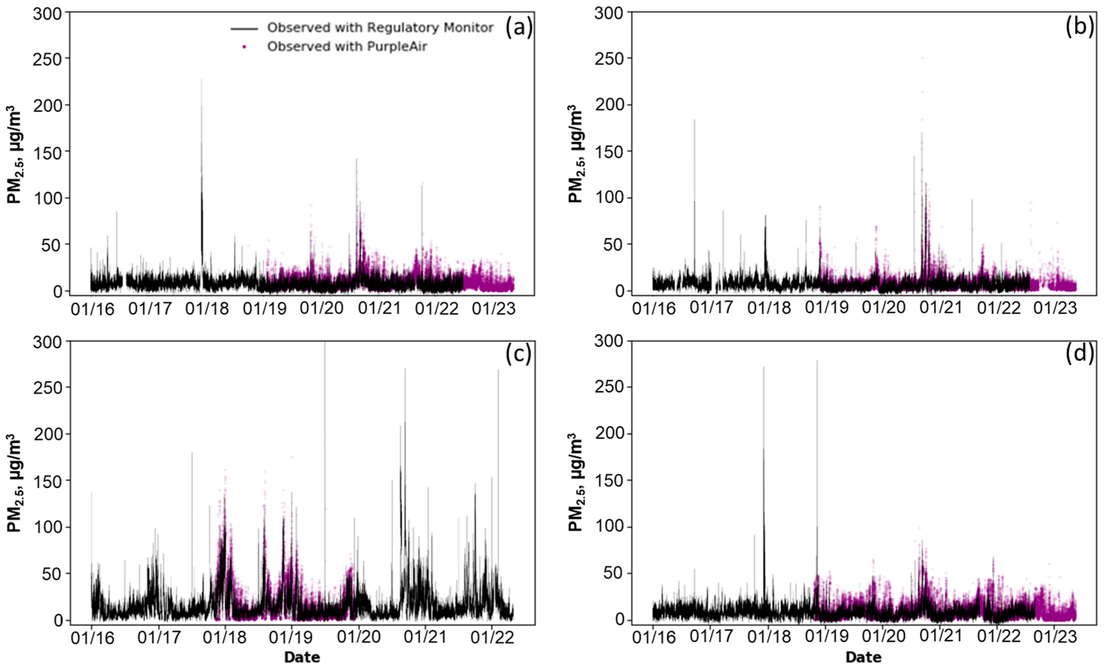
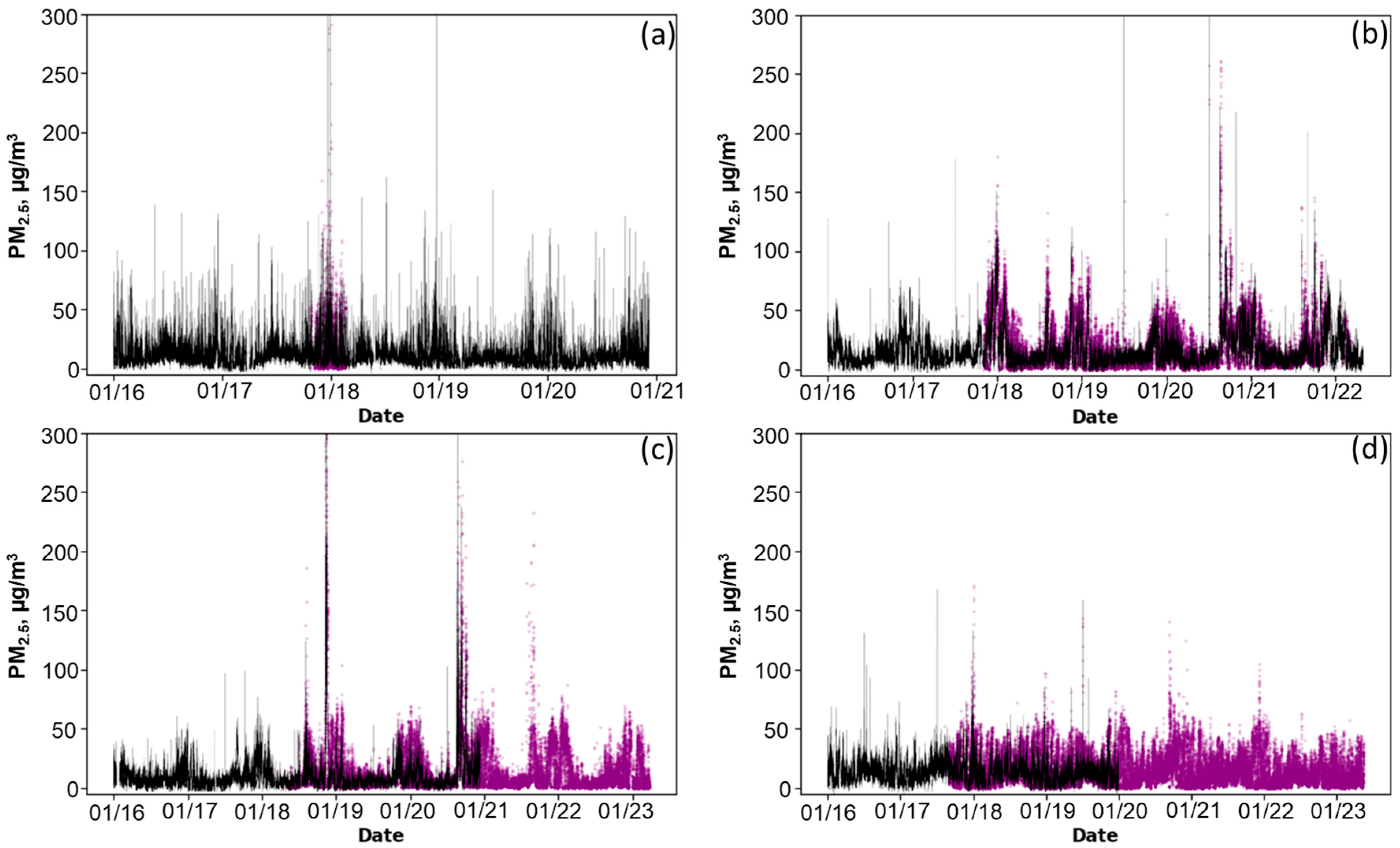
Figure 3 and Figure 4 show hourly average PM2.5, in black lines, at four FEM/FRM and four non-FEM/FRM sites and PurpleAir PM2.5 in purple dots (x-axis is in MM/YY format). From these figures, it is very clear that PurpleAir monitors captured the trend of PM2.5 at regulatory monitors from 2016 to 2022. PurpleAir observed higher PM2.5 concentrations for both FEM/FRM and non-FEM/FRM regulatory monitors. They also captured the PM2.5 events due to forest fires along with regulatory monitors. PurpleAir PM2.5 followed the trends of regulatory monitors for both less than 100 µg/m3 and greater than 100 µg/m3 PM2.5 concentrations. PM2.5 above 200 µg/m3 were captured by PurpleAir at Fresno-Garland (Figure 3c) and all non-FEM/FRM sites with the exception of one day spike at El Rio-El Rio Mesa School (Figure 3d). Spikes in PM2.5 concentrations at Sacramento-T Street (Figure 4c) were observed due to forest fire and the trend can be seen by both regulatory and PurpleAir monitors. Thus, the sensors have been able to capture local and regional episodic events.
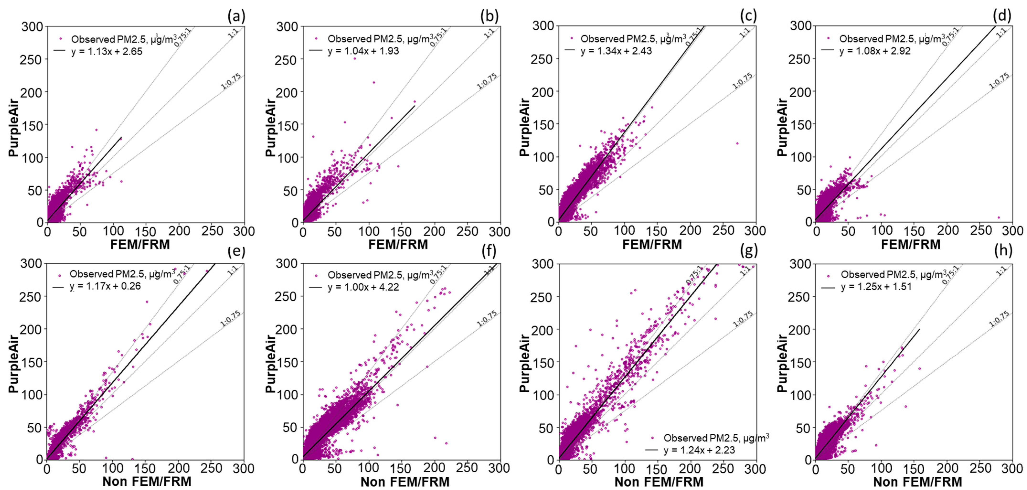
Figure 5 shows scatter plots with hourly average PurpleAir PM2.5 concentrations on the y-axis and regulatory monitored PM2.5 concentrations on x-axis. Detailed monitoring information can be found in Table 1. These plots show PurpleAir monitored higher concentrations than regulatory monitors for most of the time. Scatter plots also show +/−25% dotted lines and, for the majority of times, the scatter dots were out of +/−25% range with higher number of dots towards the y-axis or PurpleAir PM2.5. The linear fit line for all sites is on the positive side of +25%. Only El Rio School site (Figure 5b) site has shown a one-to-one linear fit.
PurpleAir-monitored PM2.5 were mostly higher than the regulatory monitored PM2.5. This may be because PurpleAir monitors were calibrated by the manufacturer using particles with completely different properties than particulate matter in the ambient air [34], and the conversion of particle counts to mass is also unknown [15]. Aside from that, it was found that the ambient air also includes water droplets with aerodynamic particle size. Traditionally, both FEM/FRM and non-FEM/FRM monitors measure PM2.5 by removing water content in the sample inlet. This was achieved by heating the sample air in the inlet pipe. However, on the contrary, PurpleAir sensors measure PM2.5 concentrations without removing moisture content in aerosols. It is the water content in the ambient air that makes PM2.5 measured by PurpleAir as an “Absolute PM2.5” or, in context to regulatory monitors, as “Wet PM2.5”. The adjustment of water content in the PurpleAir measured PM2.5 during the conversion from particle count to mass is unknown. Therefore, even before the comparison between PurpleAir PM2.5 with FEM/FRM and non-FEM/FRM monitored PM2.5, the PurpleAir PM2.5 concentrations will be greater than regulatory monitors most of the time.
Table 1 shows a statistical evaluation of PurpleAir monitors in comparison with regulatory monitors. For statistical evaluation of the PM2.5 corelation coefficient (R2), mean bias (MB) and root mean square error (RMSE) were performed. Mean bias is primarily used to estimate the average bias between two variables. The coefficient of determination, R-squared (R2), determines how well data fit the regression model compared to observation data. The Root Mean Square Error (RMSE) is a frequently used measure of the difference between two actual measures and how much error there is between two variables. Equations of the evaluation indices are shown below:
MB = 1 n i = 1 n P i R i
RMSE = 1 n i = 1 n P i R i 2
R 2 = i = 1 n P i R i i = 1 n P i i = 1 n R i n i = 1 n P i 2 ( i = 1 n P i ) 2 n i = 1 n R i 2 ( i = 1 n R i ) 2 2
where Pi is PurpleAir PM2.5 concentrations, Ri is regulatory PM2.5 concentrations, R ¯ is mean of Ri, P ¯ is mean of Pi, and n is the number of hourly samples.
For all FEM/FRM (Table 1 and Table S1), coefficient of determination, R2 values were between 0.23 and 0.9 with an average of 0.62. For all non-FEM/FRM (Table 2 and Table S2), R2 values were between 0.27 and 0.92 with an average of 0.74, which was lower than reported studies conducted for shorter durations [10,21,23]. The coefficient of determination, R2, of Goleta, El Rio-El Rio School, and Lompoc-H Street has shown the lowest values of 0.56, 0.5, and 0.6, respectively. These three sites are along the coastlines of Southern California. It is expected that the moisture content in the coastal air will be higher than the inland area. This affirms that moisture content plays a significant role in PurpleAir PM2.5 monitoring. Moisture in the air attracts PM due to its hygroscopic characteristics and results in higher concentrations. As of now, PurpleAir monitors do not heat inlet air compared to regulatory monitors. The rest of the sites, located inland, have shown higher R2 of greater than 0.70. The mean bias is highest at Fresno-Garland of 9.62 µg/m3 followed by 6.93 µg/m3 at Sacramento-T Street, as shown in Supplementary Material Tables S1 and S2. The mean bias for all sites were positive, showing higher PM2.5 from PurpleAir than FEM/FRM and non-FEM/FRM.
After validation of the performance of purple air sensors with observed daily average data, the sensor data were used to perform detailed summary statistics across different regions of California: from Bay Area Air Quality Management District (AQMD) (Bay Area), Sacramento Metropolitan AQMD (Sacramento), San Diego Air Pollution Control District (APCD) (San Diego), San Joaquin Valley APCD (San Joaquin), and South Coast AQMD (South Coast) according to the availability of data from sensors for recent years (2018–2020). After excluding poorly performing sensors (around 4%), all the purple air sensors were used in this statistical analysis. Table 2, Table 3 and Table 4 show results from this analysis.
The sensor dataset revealed a wide range of PM2.5 concentrations, with a maximum 24 h average concentration of about 200 µg/m3 measured in the Bay Area in 2020. Other northern Californian regions (Sacramento), which showed the next highest daily concentrations, were followed by the South Coast and San Diego, respectively. Dry weather [35] and forest management techniques over the past few decades have also contributed to a rise in the frequency and intensity of wildfire outbreaks in California, contributing to the severity of the 2020 fire season there. Even though they were less severe than in 2020, California experienced record-breaking wildfires in 2018, which also displayed comparable trends in all the aforementioned districts. San Diego was less affected by the wildfires. Residential fire burning and other incidents, such as fire starting from electric transmission lines, contributed to higher maximum PM2.5 concentrations in Northern California in 2019. Land–sea breezes can significantly pollute Northern California’s coastal areas. The influence of a combination of wildfires and anthropogenic emissions was felt at South Coast as well, leading to higher concentrations in this region.
Additionally, across the entire state of California, the standard deviation ranged from 8 to 30 µg/m3 for the individual counties, with higher variabilities in the northern California regions most affected by fires. The median PM2.5 concentration of the dataset was between 5 and 13 µg/m3, while the mean concentrations ranged from 7 to 30 µg/m3. Overall, the PM2.5 measurements showed higher maxima and standard deviation values in 2020 compared to 2019 or 2018, which is commiserate with the fact that wildfire intensity peaked in 2020, as previously mentioned.
A region-wise inter-comparison (Bay Area, San Diego, Sacramento, San Joaquin, and South Coast) in the State of California of the daily average of sensor data for the years 2018–2020, as seen from Table 2, Table 3 and Table 4, revealed that areas in northern California, including Bay Area, Sacramento, and San Joaquin, had distinctly higher 95th and 75th percentile concentrations in comparison to South Coast during the year of extensive wildfires in 2020. This reemphasizes the importance of wildfire impact on air pollution in the Northern California. Therefore, 2020 may be considered the year of the highest daily PM2.5 concentrations measured in California.
The number of sensors has also increased significantly, from around 369 in 2018 to around 773 sensors in 2020 in the Bay Area, a growth of a huge 110 percent. The other two areas, Sacramento and San Diego, exhibit a more modest growth of sensors (18 percent in San Diego and 94 percent in Sacramento) in comparison to the Bay Area. The southern part of California (South Coast) witnessed a growth of sensors from around 552 in 2018 to around 741 in 2020, a growth of 34 percent.
Table 5 shows the total number of daily-average (or 24 h average) PM2.5 of all sensors’ observations and exceedances in the regions of California. For all regions, in contrast to 3% in 2019 and 7% in 2018, the overall average percentage of exceedances over all regions of the state of California was almost 11% in 2020. In terms of overall exceedances in 2020, the Bay Area has the highest percentage of exceedances (58%), followed by the South Coast (21%), San Joaquin (12%), Sacramento (8%), and San Diego (1%). The South Coast had the largest percentage of exceedances in 2019 (51%), followed by the Bay Area (27%), San Joaquin (17%), Sacramento (4%), and San Diego (1%). 2018 saw the highest percentage of exceedances in the South Coast (54%), followed by the Bay Area (24%), San Joaquin (18%), and San Diego (0.7%). The analysis demonstrates the impact of COVID-19 in the South Coast in 2020, when anthropogenic emissions were lower than in 2018. However, the effects of the California wildfires were more noticeable in 2020.
To test the significance of the annual variations (2018–2020) in the distribution of daily mean PM2.5 levels, as measured by the sensors across the state of California, the non-parametric Kruskal–Wallis test was performed to determine whether the distribution of daily means was identical to each other or showed any significant difference amongst them for the years (2018–2020). The null hypothesis that many samples were taken from the same population was tested using this non-parametric technique, which is arguably the most extensively used test for this purpose. Since the null hypothesis was rejected across the years for all the regions of California, a post hoc test Dunn’s test was conducted to perform a multi-comparison analysis across all years for all regions in California to find out which samples (years) were different from each other. The Dunn’s test results from Bay Area have been displayed below for the years 2018, 2019, and 2020 as a representative result in Table 6.
The tables show that the differences in concentrations were significant across all years at the 95th confidence level (Table 4) since p = 0.00 < p = 0.05. In the case of San Diego, the differences in daily mean concentrations for 2018 and 2019, and between 2019 and 2020 were significant (p = 0.00) but there were no significant differences between 2019 and 2020 (p > 0.05). For South Coast, there were significant differences in daily mean concentrations of PM2.5 across all the years considered (p = 0.00). For San Joaquin, the differences in daily average PM2.5 concentrations over the years were significant. For Sacramento, the differences were not significant for the years 2018 and 2020 (p > 0.05) but were significant across the other years.

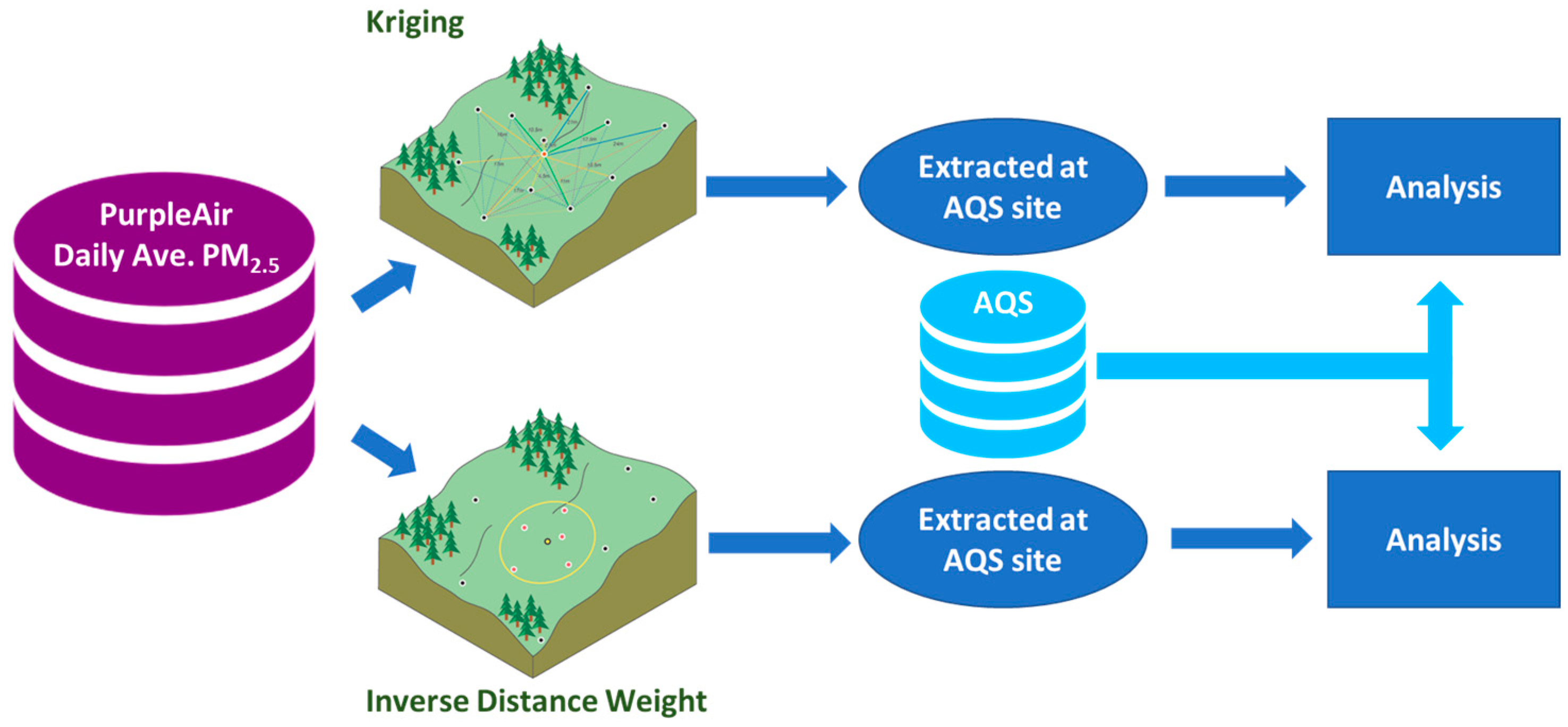
3.2. Geostatistically Predicted and Observed PM2.5

The regulatory monitoring network is too sparse to support community-scale PM2.5 exposure assessments. PurpleAir monitoring network provides more dense monitors up to community-scale and spatially across California State compared to the existing regulatory monitoring network. Geostatistical interpolation techniques—Kriging and IDW using PurpleAir PM2.5—might help to bridge the gap between PurpleAir and regulatory monitored PM2.5. Interpolation was conducted using the daily average PurpleAir PM2.5 for the years 2018 and 2020 as the PurpleAir monitoring began in California in 2016, and fewer monitors were in operation until the end of 2017. 
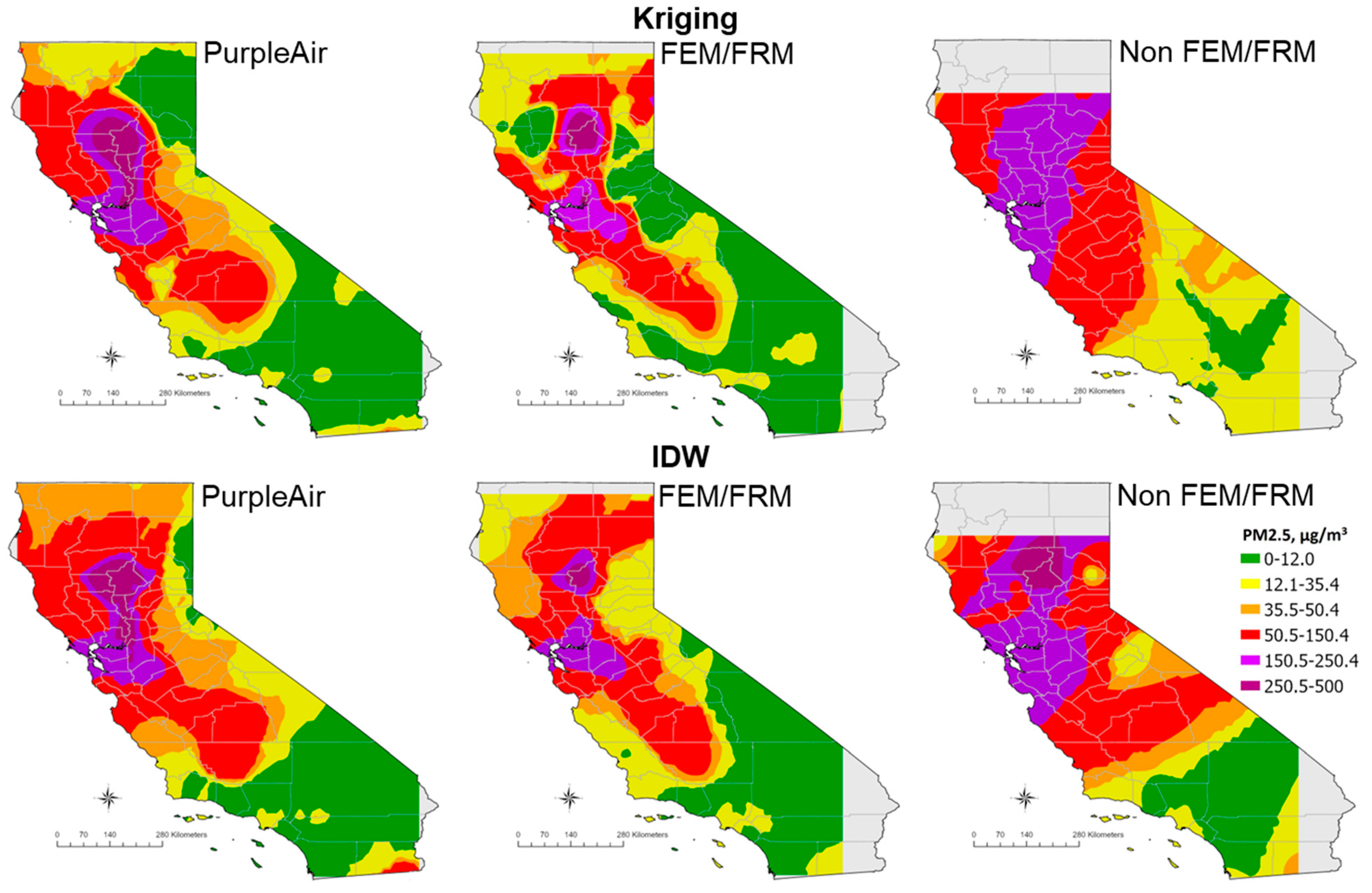
Figure 6 shows statistically interpolated PurpleAir, FEM/FRM, and non-FEM/FRM daily average PM2.5 on 16 November 2018, by Kriging and IDW. Both statistical interpolation techniques have captured the smoke dispersion from CAMP fire started on 8 November 2018 [36]. The difference in spatially interpolated daily average PurpleAir PM2.5 in the northern part of California was due to a difference in interpolation approaches by Kriging and IDW. For both years, the interpolated sensor data provided a realistic representation of daily PM2.5 concentrations and thus may reduce the uncertainty introduced by interpolation errors due to a sparse observational network of FRM and non-FRM monitors for effective decision-making. However, although the sensor data are subject to some uncertainty, as discussed earlier, the interpolated PM2.5 from PurpleAir has shown a better representation of PM2.5 due to the dense number of PM2.5 monitors for interpolation in comparison to the thinly distributed network of FEM/FRM and non-FEM/FRM monitors. For further analysis, four regulatory sites across California State without monitors were selected for its assessment. The reason for not selecting collocated monitored sites was to avoid the influence of monitored PurpleAir PM2.5 at the same location.
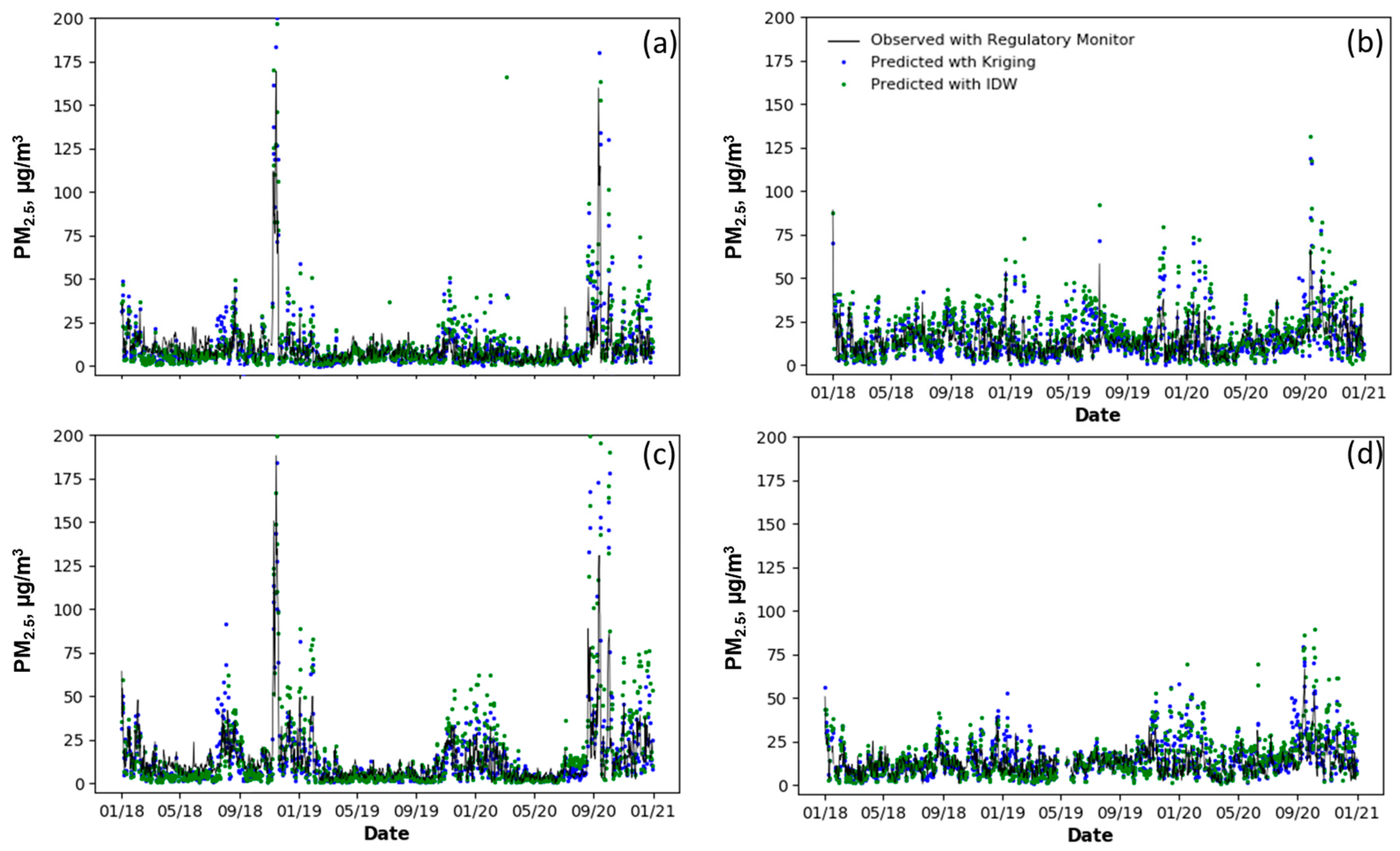
Figure 7 shows observed daily average PM2.5 concentrations in black lines and interpolated PM2.5 concentrations at the four above-mentioned regulatory monitoring sites (x-axis is in MM/YY format). The time-series plots show a good agreement between observed and interpolated PM2.5. Both IDW and Kriging methods captured the peaks of observed PM2.5. However, for many days, Kriging and IDW over-predicted the PM2.5, as shown in Figure 7. The reason of the over prediction can be due to higher observed PM2.5 by PurpleAir monitors. Scatter plots with interpolated PM2.5 on y-axis and regulatory on x-axis show good agreement, and most of the interpolated falls between +/−25%. Both Kriging and IDW geo-statistically demonstrated that these can be used to interpolated daily average PurpleAir PM2.5 at unmonitored locations for exposure and air quality assessments. The agreement between geo-statistically interpolated PurpleAir and observed daily average PM2.5 gives confidence in using PurpleAir PM2.5 with regulatory monitors to estimate PM2.5 at unmonitored locations. This demonstrates that low-cost PM2.5 sensors have a potential to fill in the gaps in the regulatory monitoring networks and might be useful to overcome the limitations and improve the air quality assessments and other scientific assessments. These PurpleAir PM2.5 can be integrated and used with observed regulatory PM2.5 to formulate a decision support system using geostatistical techniques, but before that, the uncertainty due to sensor measurements should be minimized prior to their usage to supplement regulatory monitors.
Table 7 shows a statistical evaluation of interpolated daily averaged PurpleAir PM2.5, using Kriging and IDW techniques, with daily averaged observed PM2.5 concentrations. The interpolated PM2.5 by Kriging has lower Root Mean Square Error (RMSE) and Mean Bias (MB) values than IDW. Corelation co-efficient values for the Oakland-West and Stockton-Hazelton sites were above 0.76 and were lower for the Mira Loma and Otay Mesa sites.

4. Conclusions

Recently emerged low-cost sensor-based monitoring technology has given a new dimension to air quality monitoring. Due to their portability and low-cost, sensors have made community-based micro-environment monitoring of air pollutants possible by providing access to local community members and enabling them to be a part of the air quality monitoring process. Currently, PurpleAir monitoring network is the densest sensor-based PM2.5 monitoring network that exists on a global scale. This sensor-based network has successfully achieved the objectives of educating the community about air pollution and helped alert the community for higher PM2.5 concentrations due to incidents such as forest fires on account of its high density of air quality sensors. However, due to the lack of best operational procedures, practices, and guidelines, this publicly available dataset cannot be used without QA/QC for air quality and other scientific assessments. The evaluation of PurpleAir PM2.5 for California State conducted in this study included QA/QC procedures, assessment with reference to monitored PM2.5 concentrations, and the formulation of a decision support system integrating these sensor-based observations using geostatistical techniques.
The hourly and daily average observed PM2.5 concentrations from PurpleAir monitors generally followed the trends of observed PM2.5 levels at regulatory monitors. PurpleAir monitored PM2.5 also captured essential peaks of PM2.5 concentrations due to incidents such as forest fires over the fire-year period. In comparison with reference-monitored PM2.5 levels, it was found that PurpleAir PM2.5 concentrations were mostly higher. For longer time periods, the correlation coefficient R2 values were between 0.54 and 0.86 for selected collocated PurpleAir for both FEM/FRM and non-FEM/FRM monitors.
PurpleAir monitors can fill in a void in the data representation of PM2.5 predictions on a localized scale. The methods of Kriging and IDW show similar patterns on spatial and temporal interpolation from PurpleAir PM2.5, but before that, the uncertainty due to sensor measurements should be minimized prior to their usage to supplement regulatory monitors. Still, low-cost sensor-based monitors need to be integrated with regulatory monitors to provide higher spatio-temporal observed data for regulatory and policy purposes. They are great tools at local community levels to assess air quality and build awareness amongst citizens on risks of air pollution. This is evident in this study, as seen in the substantial increase in sensors across California over the years. Although there is an overall decrease in PM2.5 concentrations, there are still problem areas due to wildfires in Northern California and local air pollution in Southern California which require further thinking and the development of mitigation strategies to retrieve the situations. The high number of sensors would help in enhancing the spatial density of observations. Overall, this study revealed that, despite its shortcomings, low-cost PurpleAir sensor-based measurements could be an effective tool for ambient air quality monitoring. The efficacy of the application of low-cost sensors in this study implies that sensor networks may be broadened worldwide, especially in developing countries where there is a scarcity of regulatory air quality monitors to investigate high PM2.5 concentrations. This would entail building a global roadmap for the scientific community on the usage of these sensors for air quality assessments and their subsequent impact on human health.

Supplementary Materials

The following supporting information can be downloaded at: https://www.mdpi.com/article/10.3390/pollutants3040033/s1, Table S1: Statistical assessment of hourly average PurpleAir PM2.5 at selected sites for the years 2016 and 2022 at FEM/FRM; Table S2: Statistical assessment of hourly average PurpleAir PM2.5 at selected sites for the years 2016 and 2022 at non-FEM/FRM.

Author Contributions

Authors individual contributions are as: Conceptualization, methodology. Z.F. and J.B.; software, Z.F. and J.S.; validation, writing, review and editing. J.B.; formal analysis, Z.F., J.B. and J.S.; data curation, visualization. Z.F.; writing—original draft preparation, Z.F. All authors have read and agreed to the published version of the manuscript.

Funding

The work was independent research, and no funding was received.

Data Availability Statement

PurpleAir and EPA AQS data are all publicly available data.

Conflicts of Interest

The authors declare no conflict of interest.

References

  1. Pope, C.A.; Ezzati, M.; Dockery, D.W. Fine-Particulate Air Pollution and Life Expectancy in the United States. N. Engl. J. Med. 2009, 360, 376–386. [Google Scholar] [CrossRef] [PubMed]
  2. Chen, X.C.; Jahn, H.J.; Engling, G.; Ward, T.J.; Kraemer, A.; Ho, K.F.; Yim, S.H.L.; Chan, C.Y. Chemical characterization and sources of personal exposure to fine particulate matter (PM2.5) in the megacity of Guangzhou, China. Environ. Pollut. 2017, 231, 871–881. [Google Scholar] [CrossRef] [PubMed]
  3. Pozzer, A.; Bacer, S.; Sappadina, S.Z.; Predicatori, F.; Caleffi, A. Long-term concentrations of fine particulate matter and impact on human health in Verona, Italy. Atmos. Pollut. Res. 2019, 10, 731–738. [Google Scholar] [CrossRef]
  4. Pope, C.A.; Dockery, D.W. Health effects of fine particulate air pollution: Lines that connect. J. Air Waste Manag. Assoc. 2006, 56, 709–742. [Google Scholar] [CrossRef]
  5. Shou, Y.; Huang, Y.; Zhu, X.; Liu, C.; Hu, Y.; Wang, H. A review of the possible associations between ambient PM2.5 exposures and the development of Alzheimer’s disease. Ecotoxicol. Environ. Saf. 2019, 174, 344–352. [Google Scholar] [CrossRef]
  6. Ghosh, S.; Biswas, J.; Guttikunda, S.K.; Roychowdhury, S. An investigation of potential regional and local source regions affecting fine particulate matter concentrations in Delhi, India. J. Air Waste Manag. Assoc. 2015, 65, 218–231. [Google Scholar] [CrossRef]
  7. Pinto, J.P.; Lefohn, A.S.; Shadwick, D.S. Spatial Variability of PM2.5 in Urban Areas in the United States. J. Air Waste Manag. Assoc. 2004, 54, 440–449. [Google Scholar] [CrossRef]
  8. Wang, Y.; Li, J.; Jing, H.; Zhang, Q.; Jiang, J.; Biswas, P. Laboratory Evaluation and Calibration of Three Low-Cost Particle Sensors for Particulate Matter Measurement. Aerosol Sci. Technol. 2015, 49, 1063–1077. [Google Scholar] [CrossRef]
  9. U.S. Environmental Protection Agency (U.S. EPA). EPA Scientists Develop Federal Reference & Equivalent Methods for Measuring Key Air Pollutants. Available online: https://www.epa.gov/airresearch/epa-scientists-develop-federal-reference-equivalentmethods-measuring-key-air (accessed on 9 October 2020).
  10. Gupta, P.; Doraiswamy, P.; Levy, R.; Pikelnaya, O.; Maibach, J.; Feenstra, B.; Polidori, A.; Kiros, F.; Mills, K.C. Impact of California fires on local and regional air quality: The role of a low-cost sensor network and satellite observations. GeoHealth 2018, 2, 172–181. [Google Scholar] [CrossRef]
  11. Wallace, L.; Zhao, T. Spatial Variation of PM2.5 Indoors and Outdoors: Results from 261 Regulatory Monitors Compared to 14,000 Low-Cost Monitors in Three Western States over 4.7 Years. Sensors 2023, 23, 4387. [Google Scholar] [CrossRef]
  12. Bi, J.; Wildani, A.; Chang, H.H.; Liu, Y. Incorporating low-cost sensor measurements into high-resolution PM2.5 modeling at a large spatial scale. Environ. Sci. Technol. 2020, 54, 2152–2162. [Google Scholar] [CrossRef] [PubMed]
  13. Morawska, L.; Thai, P.K.; Liu, X.; Asumadu-Sakyi, A.; Ayoko, G.; Bartonova, A.; Bedini, A.; Chai, F.; Christensen, B.; Dunbabin, M.; et al. Applications of low-cost sensing technologies for air quality monitoring and exposure assessment: How far have they gone? Environ. Int. 2018, 116, 286–299. [Google Scholar] [CrossRef] [PubMed]
  14. Williams, R.; Nash, D.; Hagler, G.; Benedict, K.; MacGregor, I.; Seay, B.; Lawrence, M.; Dye, T. Peer Review and Supporting Literature Review of Air Sensor Technology Performance Targets; EPA/600/R-18/324; EPA Technical Report Undergoing Final External Peer Review; EPA: Washington, DC, USA, 2018.
  15. Farooqui, M.Z.; Biswas, J.; Roychoudhry, S.; Ghosh, S. Evaluation of low-cost sensor for PM2.5 Assessment: A case study of California State. In Proceedings of the A&WMA’s 113th Virtual Annual Conference & Exhibition, San Francisco, CA, USA, 30 June–2 July 2020. [Google Scholar]
  16. Gao, M.; Cao, J.; Seto, E. A distributed network of low-cost continuous reading sensors to measure spatiotemporal variations of PM2.5 in Xi’an, China. Environ. Pollut. 2015, 199, 56–65. [Google Scholar] [CrossRef]
  17. Stavroulas, I.; Grivas, G.; Michalopoulos, P.; Liakakou, E.; Bougiatioti, A.; Kalkavouras, P.; Fameli, K.M.; Hatzianastassiou, N.; Mihalopoulos, N.; Gerasopoulos, E. Field Evaluation of Low-Cost PM Sensors (Purple Air PA-II) Under Variable Urban Air Quality Conditions, in Greece. Atmosphere 2020, 11, 926. [Google Scholar] [CrossRef]
  18. Mukherjee, A.; Brown, S.G.; McCarthy, M.C.; Pavlovic, N.R.; Stanton, L.G.; Snyder, J.L.; D’Andrea, S.; Hafner, H.R. Measuring Spatial and Temporal PM2.5 Variations in Sacramento, California, Communities Using a Network of Low-Cost Sensors. Sensors 2019, 19, 4701. [Google Scholar] [CrossRef] [PubMed]
  19. Zikova, N.; Hopke, P.K.; Ferro, A.R. Evaluation of new low-cost particle monitors for PM2.5 concentrations measurements. J. Aerosol Sci. 2017, 105, 24–34. [Google Scholar] [CrossRef]
  20. Ardon-Dryer, K.; Dryer, Y.; Williams, J.N.; Moghimi, N. Measurements of PM2.5 with PurpleAir under atmospheric conditions. Atmos. Meas. Tech. 2020, 13, 5441–5458. [Google Scholar] [CrossRef]
  21. South Coast Air Quality Management District (SCAQMD); Air Quality Sensor Performance Evaluation Center (AQ-SPEC). Available online: http://www.aqmd.gov/aq-spec/evaluations/summary-pm (accessed on 29 September 2020).
  22. Robinson, D.L. Accurate, Low Cost PM2.5 Measurements Demonstrate the Large Spatial Variation in Wood Smoke Pollution in Regional Australia and Improve Modeling and Estimates of Health Costs. Atmosphere 2020, 11, 856. [Google Scholar] [CrossRef]
  23. Land Regional Air Protection Agency (LRAPA). PurpleAir Monitor Correction Factor History. Available online: https://www.lrapa.org/DocumentCenter/View/4147/PurpleAir-Correction-Summary (accessed on 11 February 2021).
  24. Sayahi, T.; Butterfield, A.; Kelly, K.E. Long-term field evaluation of the Plantower PMS low-cost particulate matter sensors. Environ. Poll. 2019, 245, 932–940. [Google Scholar] [CrossRef]
  25. Malings, C.; Tanzer, R.; Hauryliuk, A.; Saha, P.K.; Robinson, A.L.; Presto, A.A.; Subramanian, R. Fine particle mass monitoring with low-cost sensors: Corrections and long-term performance evaluation. Aerosol Sci. Tech. 2020, 54, 160–174. [Google Scholar] [CrossRef]
  26. Mei, H.; Han, P.; Wang, Y.; Zeng, N.; Liu, D.; Cai, Q.; Deng, Z.; Wang, Y.; Pan, Y.; Tang, X. Field evaluation of low-cost particulate matter sensors in Beijing. Sensors 2020, 20, 4381. [Google Scholar] [CrossRef]
  27. Kuula, J.; Mäkelä, T.; Hillamo, R.; Timonen, H. Response characterization of an inexpensive aerosol sensor. Sensors 2017, 17, 2915. [Google Scholar] [CrossRef] [PubMed]
  28. U.S. Environmental Protection Agency (U.S. EPA). NAAQS Table. Available online: https://www.epa.gov/criteria-air-pollutants/naaqs-table (accessed on 11 August 2023).
  29. California Air Resources Board. Maps of State and Federal Area Designations. Available online: https://ww2.arb.ca.gov/resources/documents/maps-state-and-federal-area-designations (accessed on 11 August 2023).
  30. Lu, G.Y.; Wong, D.W. An adaptive inverse-distance weighting, spatial interpolation technique. Comput. Geosci. 2008, 34, 1044–1055. [Google Scholar] [CrossRef]
  31. Cressie, N. Statistics for Spatial Data; Wiley: New York, NY, USA, 1991; ISBN 0-471-00255-0. [Google Scholar]
  32. U.S. Environmental Protection Agency. Air Quality System. Available online: https://aqs.epa.gov/aqsweb/documents/data_mart_welcome.html (accessed on 27 February 2020).
  33. Ryu, J.; Kim, M.; Cha, K.; Lee, T.H.; Choi, D. Kriging interpolation methods in geostatistics and DACE model. KSME Int. J. 2002, 16, 619–632. [Google Scholar] [CrossRef]
  34. Badura, M.; Batog, P.; Drzeniecka-Osiadacz, A.; Modzel, P. Evaluation of Low-Cost Sensors for Ambient PM2.5 Monitoring. J. Sens. 2018, 2018, 5096540. [Google Scholar] [CrossRef]
  35. Keeley, J.E.; Syphard, A.D. Large California wildfires: 2020 fires in historical context. Fire Ecol. 2021, 17, 2–11. [Google Scholar] [CrossRef]
  36. California Fire. Available online: https://www.fire.ca.gov/incidents/2018/11/8/camp-fire (accessed on 5 June 2020).
Figure 1. PurpleAir and regulatory monitoring sites in California State.
Pollutants 03 00033 g001
Figure 2. Flow chart of geostatistical interpolation of daily average PurpleAir PM2.5.
Pollutants 03 00033 g002
Figure 3. Time-series plots of PM2.5 at FEM/FRM monitoring site with nearby PurpleAir monitors (a) Goleta (b) Lompoc-H St. (c) Fresno-Garland and (d) El Rio-El Rio Mesa School.
Pollutants 03 00033 g003
Figure 4. Time-series plots of PM2.5 at non-FEM/FRM monitoring site with nearby PurpleAir monitors (a) Calexico-Ethel St. (b) Bakersfield-California Ave. (c) Sacramento-T St. and (d) Riverside-Rubidoux.
Pollutants 03 00033 g004
Figure 5. Scatter plots of PM2.5 at FEM/FRM monitoring site with nearby PurpleAir monitors (a) Goleta (b) Lompoc-H St. (c) Fresno-Garland and (d) El Rio-El Rio Mesa School Ethel St. (e) Calexico-Ethel St. (f) Bakersfield-California Ave. (g) Sacramento-T St. (h) Riverside-Rubidoux.
Pollutants 03 00033 g005
Figure 6. Statistically interpolated daily average PurpleAir PM2.5 across California State on 16 November 2018, by Kriging and IDW.
Pollutants 03 00033 g006
Figure 7. Time-series plot of statistically predicted and observed daily average PM2.5 concentrations at (a) Oakland-West, (b) Mira Loma, (c) Stockton-Hazelton, and (d) Otay Mesa.
Pollutants 03 00033 g007
Table 1. Statistical assessment of hourly average PurpleAir PM2.5 at selected sites for the years 2016 and 2022 at FEM/FRM and non-FEM/FRM sites.
Site Name and AQS ID, POCPurpleAir Sensor IndexDistance, mtsDates DurationNum. of Paired Observation (#)R2Mean Bias (µg/m3)RMSE
FEM/FRM
El Rio-Rio Mesa Schl. 061113001, 395940.182 April 2016 to 31 August 202230,7980.503.57.85
Fresno-Garland 060190011, 323581.8731 July 2017 to 9 December 2019 17,1940.835.711.85
Goleta-Fairview 060832011, 116,705029 September 2018 to 30 June 2022 28,5320.563.46.93
Lompoc 060832004, 116,703029 September 2018 to 30 June 202228,4820.602.16.21
non-FEM/FRM
Bakersfield 060290014, 323500.631 July 2017 to 8 March 201934,5830.734.311.70
Calexico-Ethel Street 060250005, 311740.024 October 2017 to 2 February 201824860.893.511.60
Sacramento-T Street 060670010, 384402.12 February 2019 to 11 December 202014,7970.864.210.20
Riverside 060658001, 918548.510 July 2017 to 31 December 201914,6040.695.79.70
Table 2. All sensors daily average PM2.5 summary over different regions in California for the year 2018.
Bay AreaSacramento MetroSan DiegoSan JoaquinSouth Coast
Observations31,1302219235511,234103,236
Minimum0.310.360.510.310.32
Maximum19819773192190
Mean14.5718.9312.9520.1515.05
Std. Error of Mean0.140.570.20.190.04
Median6.5910.9710.7212.7812.04
Std. Deviation24.326.79.620.111.4
Skewness3.93.841.261.951.57
Std. Error of Skewness0.010.050.050.020.01
Kurtosis17.78181.795.935.29
Std. Error of Kurtosis0.030.10.10.050.02
Percentile 2534667
Percentile 50711111312
Percentile 751524172821
Percentile 903138274731
Percentile 955653325936
Table 3. All sensors daily average PM2.5 summary over different regions in California for year 2019.
Bay AreaSacramento MetroSan DiegoSan JoaquinSouth Coast
Observations184,6628918523924,497115,764
Minimum0.310.320.310.320.3
Maximum18510062155185
Mean7.269.9910.9112.6313.28
Std. Error of Mean0.020.130.120.10.03
Median4.955.579.147.6110.43
Std. Deviation812.48.31511.2
Skewness3.492.781.8432.22
Std. Error of Skewness0.010.030.030.020.01
Kurtosis21.79.845.0611.899.38
Std. Error of Kurtosis0.010.050.070.030.01
Percentile 2523545
Percentile 50569710
Percentile 75811141417
Percentile 901526202927
Percentile 952236274434
Table 4. The daily average PM2.5 summary of all sensors over different regions in California for the year 2020.
Bay AreaSacramento MetroSan DiegoSan JoaquinSouth Coast
Observations457,92427,37714,12431,743155,801
Minimum0.30.30.310.330.31
Maximum200198187199195
Mean14.5821.8914.1426.5316.48
Std. Error of Mean0.030.170.110.170.04
Median7.0610.3611.1314.5911.8
Std. Deviation22.828.613.230.516.6
Skewness4.112.772.932.312.96
Std. Error of Skewness00.010.020.010.01
Kurtosis21.059.8114.466.8715.12
Std. Error of Kurtosis0.010.030.040.030.01
Percentile 2534666
Percentile 50710111412
Percentile 751530183821
Percentile 903452276235
Percentile 955072378246
Table 5. Daily average observations and exceedances of all sensors in regions of California during years 2018–2020.
Total Daily ObservationsTotal Daily Exceedances Total Daily ObservationsTotal Daily Exceedances Total Daily ObservationsTotal Daily Exceedances
202020192018
Bay Area457,92443,383184,662303331,1302699
Sacramento27,377579489184822219299
San Diego14,124795523911623550.78
San Joaquin31,743876424,497188411,2342152
South Coast155,80115,468115,7645548103,2366215
Table 6. Dunn’s test for area in California for the years 2018–2020.
Sample Year 1-Sample Year 2Test StatisticStd. ErrorStd. Test StatisticSig.
Bay Area
2018–2019−64,059.51197.3−53.50.000
2019–202079,655.9538.7147.90.000
2018–202015,596.41144.613.60.000
Sacramento Metro
2018–2019−4862.3263.8−18.40.000
2019–20205418.8135.640.00.000
2018–2020556.5245.42.30.023
San Joaquin
2018–2019−8310.5226.9−36.60.000
2019–202010,625.7169.362.80.000
2018–20202315.2218.610.60.000
South Coast
2018–2019−21,381.8499.1−42.80.000
2019–202017,860.4452.439.50.000
2018–2020−3521.3467.9−7.50.000
San Diego
2018–2019−1272.6157.0−8.10.000
2019–20201495.3102.414.60.000
2018–2020222.7140.91.60.114
Table 7. Performance evaluation of statistically predicted and observed PM2.5 concentrations at selected sites in California.
Oakland-WestStockton-Haz.Mira LomaOtay Mesa
IDWKrigingIDWKrigingIDWKrigingIDWKriging
No. of Pairs10841084107910791083108310521052
Mean Bias (µg/m3)2.481.303.460.784.531.042.892.35
RMSE12.4911.5415.7713.199.787.728.387.94
R20.820.830.790.770.690.630.590.50
Disclaimer/Publisher’s Note: The statements, opinions and data contained in all publications are solely those of the individual author(s) and contributor(s) and not of MDPI and/or the editor(s). MDPI and/or the editor(s) disclaim responsibility for any injury to people or property resulting from any ideas, methods, instructions or products referred to in the content.

