Control of PMSM Based on Switched Systems and Field-Oriented Control Strategy

Abstract

Starting from the problem of studying the parametric robustness in the case of the control of a permanent magnet-synchronous motor (PMSM), although robust control systems correspond entirely to this problem, due to the complexity of the algorithms of the robust type, in this article the use of switched systems theory is proposed as a study option, given the fact that these types of systems are suitable both for the study of systems with variable structure and for systems with significant parametric variation under conditions of lower complexity of the control algorithms. The study begins by linearizing a PMSM model at a static operating point and continues with a systematic presentation of the basic elements and concepts concerning the stability of switched systems by applying these concepts to the control system of a PMSM based on the field-oriented control (FOC) strategy, which usually changes the value of its parameters during operation (stator resistance R_s, stator inductances L_d and L_q, but also combined inertia of PMSM rotor and load J). The numerical simulations performed in Simulink validate the fact that, for parametric variations of the PMSM structure, the PMSM control switched systems preserve qualitative performance in terms of its control. A series of Matlab programs are presented based on the YALMIP toolbox to obtain P_i matrices, by solving Lyapunov–Metzler type inequalities, and using dwell time to demonstrate stability, as well as the qualitative study of the performance of PMSM control switched systems by presenting in phase plane and state space analysis of the evolution of state vectors: ω PMSM rotor speed, i_q current, and i_d current.

1. Introduction

Simultaneously with the development of interest in PMSM, due to undeniable construction and performance advantages, PMSM control systems and their applications have been developed in areas such as robotics, CNC machines, computer peripherals, and aerospace engineering. These require both high performance of the control system and parametric robustness in the sense of performance preservation in case of significant variation of PMSM parameters [1,2,3,4].

Common control strategies for PMSM include FOC and direct torque control (DTC) [5,6,7,8]. If the DTC strategy provides acceptable performance but with a relatively simple control system, the FOC strategy provides both superior control performance and a control structure that can be implemented in low- and medium-cost embedded systems.

Different types of control systems can provide high performance, but variable costs of implementation in embedded systems have been developed and implemented in a particular manner depending on the applications and requirements of the PMSM control system. Thus, one can mention adaptive [9,10], predictive [11,12], and sliding mode control (SMC) [13,14], as well as neuro-fuzzy [15,16] and computational intelligence-based control systems [17,18].

In terms of parametric robustness, robust control systems [19,20,21] have obviously been developed and implemented with excellent results, but the complexity of robust computational algorithms should not be neglected.

Switched systems are characterized by the fact that at certain moments of time, under the action of a switching signal, they can change their structure or parameter values. Thus, if the system changes its parameter values within a relatively large range, the use of switched systems theory [22,23,24,25,26,27,28] can be an alternative approach to the study of parametric robustness under the circumstances of a decrease in the complexity of the implemented algorithms.

This paper presents the FOC control strategy for the control of a PMSM by emphasizing very good control performance on the condition that implementation in an embedded system proves to be easy [29]. Elements of switched systems theory are also used to study parametric robustness.

Among the YALMIP toolbox facilities we can mention specialized solvers for the classes of problems to which it is applied, and a unitary explanation of the way to use the syntax. The studies from [30,31,32,33] were written especially by the YALMIP toolbox developers and were chosen as examples of problem classes regarding automatic robust convex programming and explicit model-predictive control (MPC) for linear parameter-varying (LPV) systems used for stability and optimality. With the help of the YALMIP toolbox, Lyapunov–Metzler-type inequalities can be solved, which is the way to demonstrate the stability of switched systems.

Compared to other elements of qualitative analysis for systems stability with time-varying parameters, among which we can list Kharitonov’s theorem, the Nyquist stability criterion, and the Bode characteristics with other design elements of robust controllers for PMSM presented in [34], solving the Lyapunov–Metzler-type inequalities can produce information regarding system stability even under the conditions of some parametric and structural changes.

The main contributions of this paper can be summarized as follows:

• PMSM model linearization at a static operating point;
• Basic elements and concept summary of switched-systems stability;
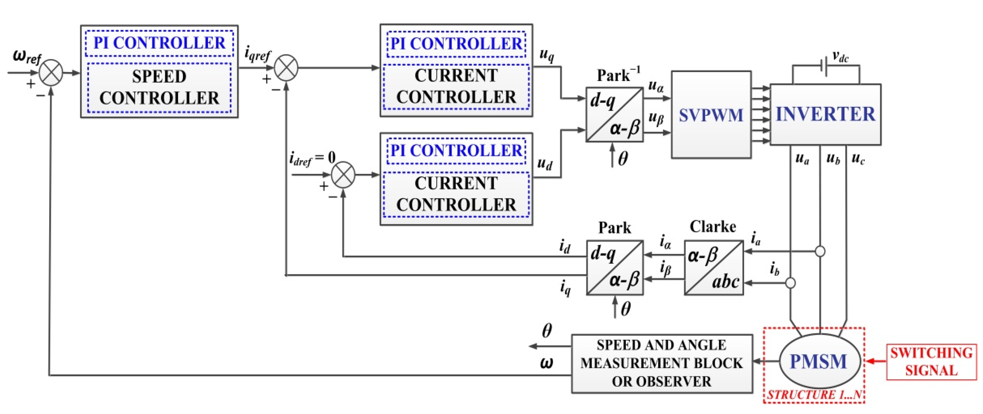
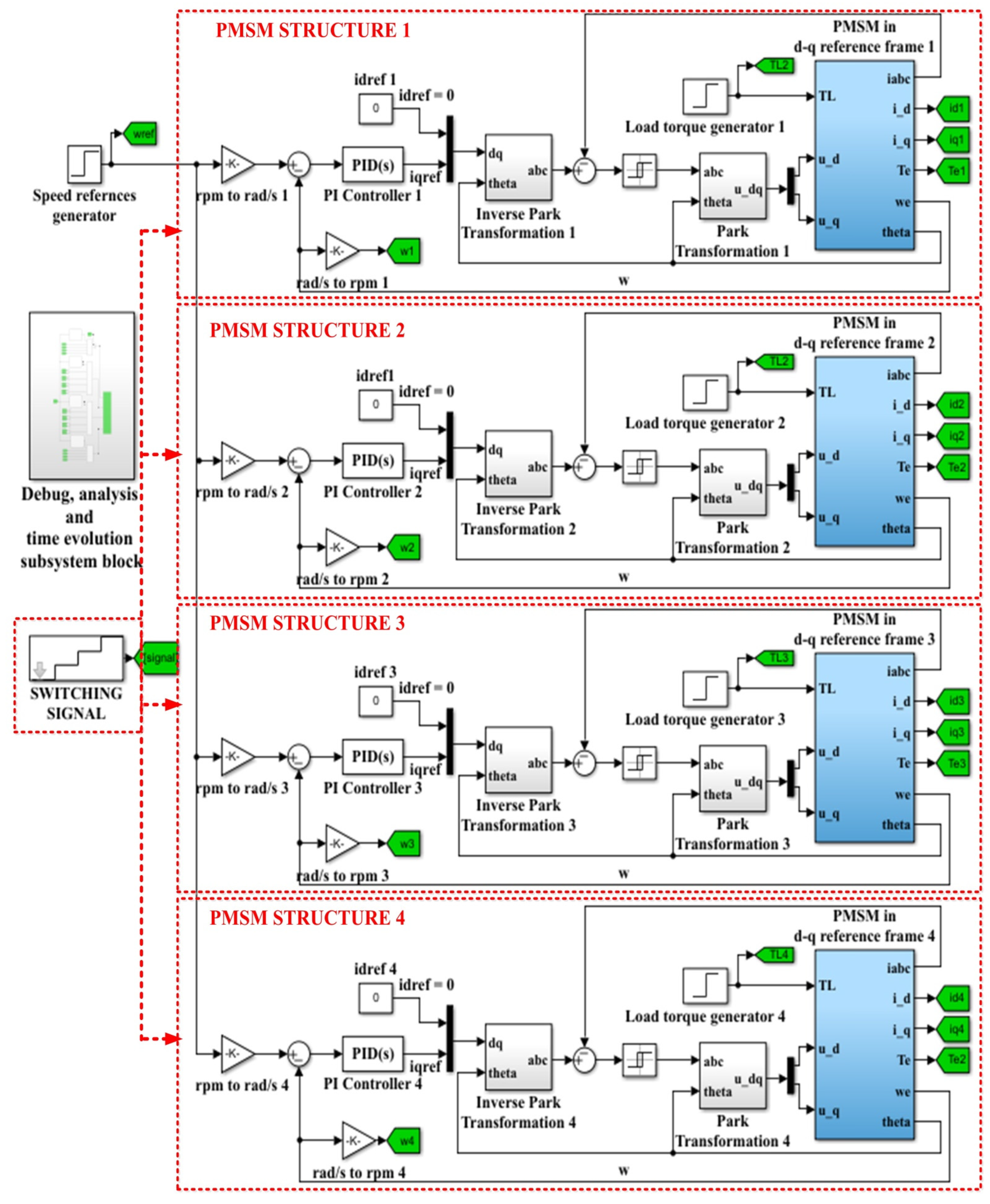
• Application of FOC control strategy and control switched systems for the control of a PMSM under significant variation of parameters that usually change value during operation (stator resistance R_s, stator inductances L_d and L_q, but also combined inertia of PMSM rotor and load J);
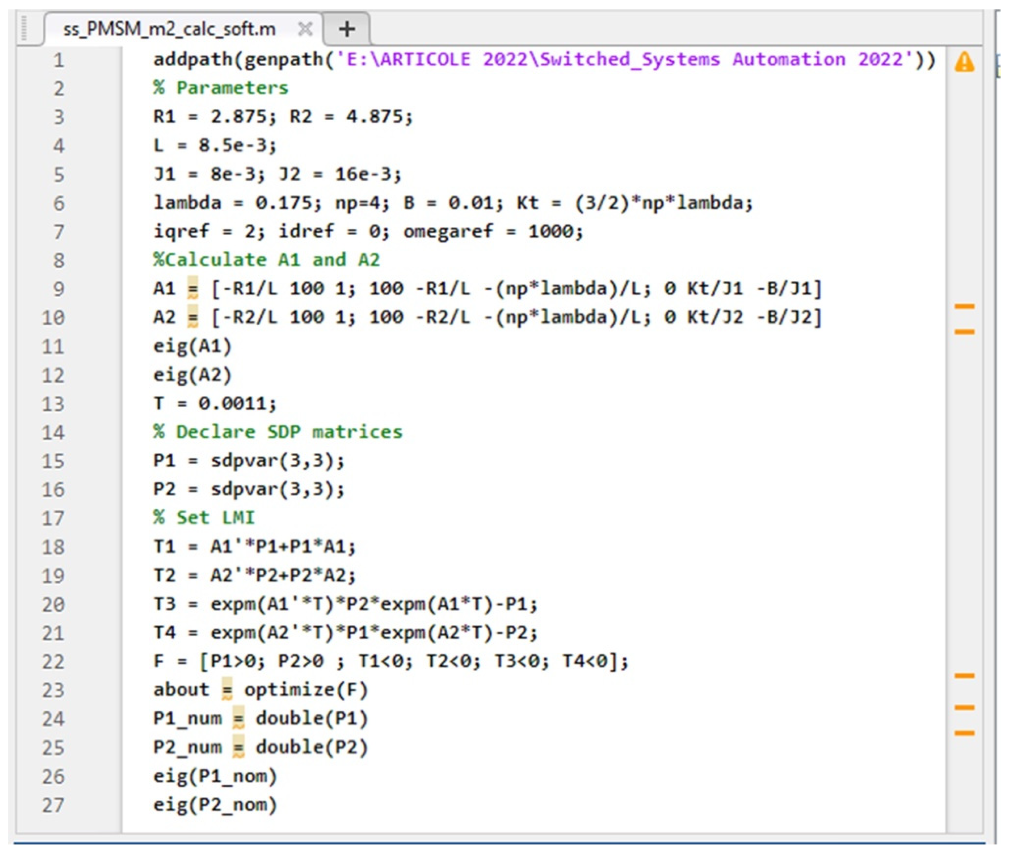
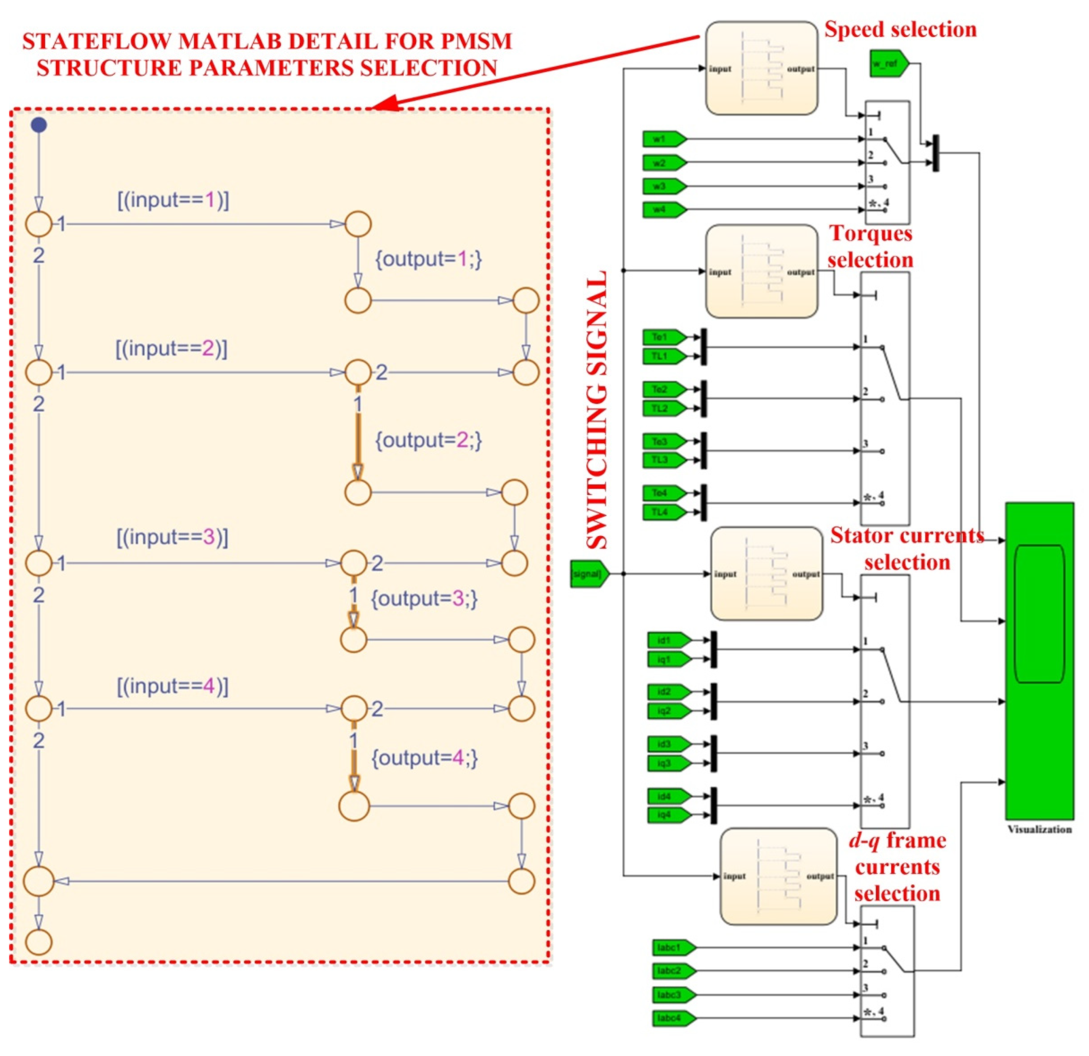
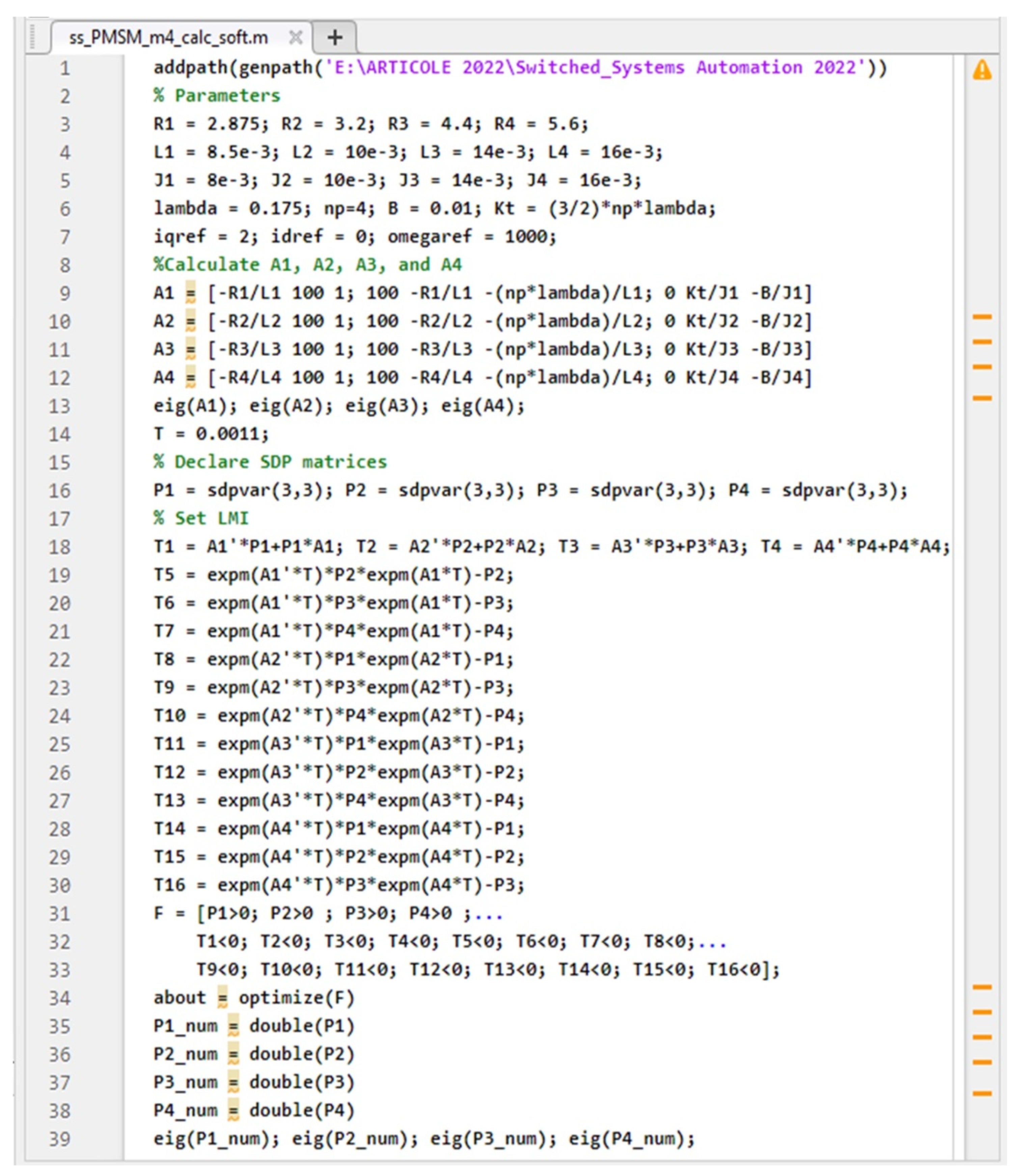
• Matlab/Simulink program implementation for calculation of the control system characteristic matrices under parametric variations, calculation of the positive definite matrices P_i from Lyapunov–Metzler inequalities to demonstrate system stability;
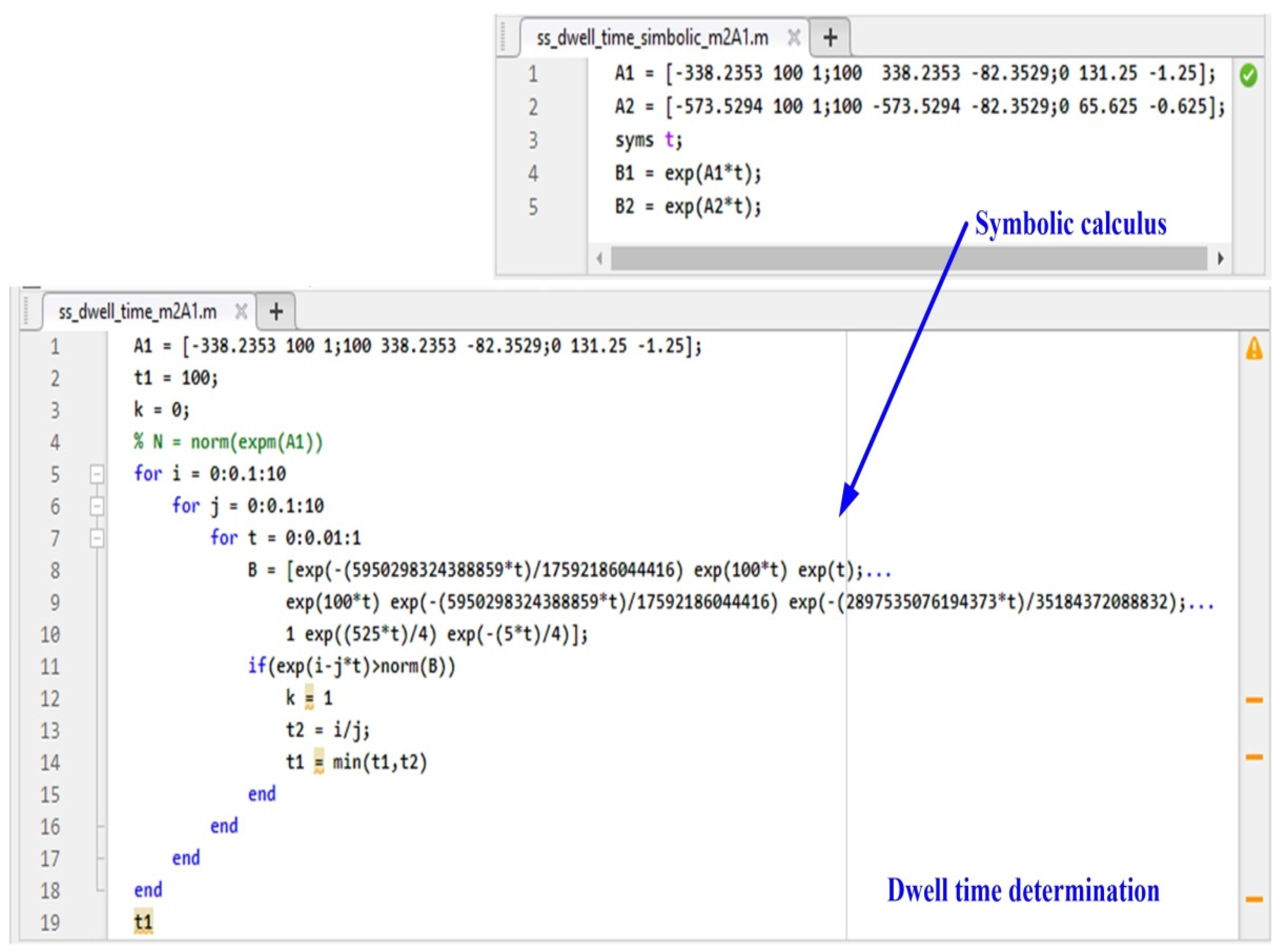
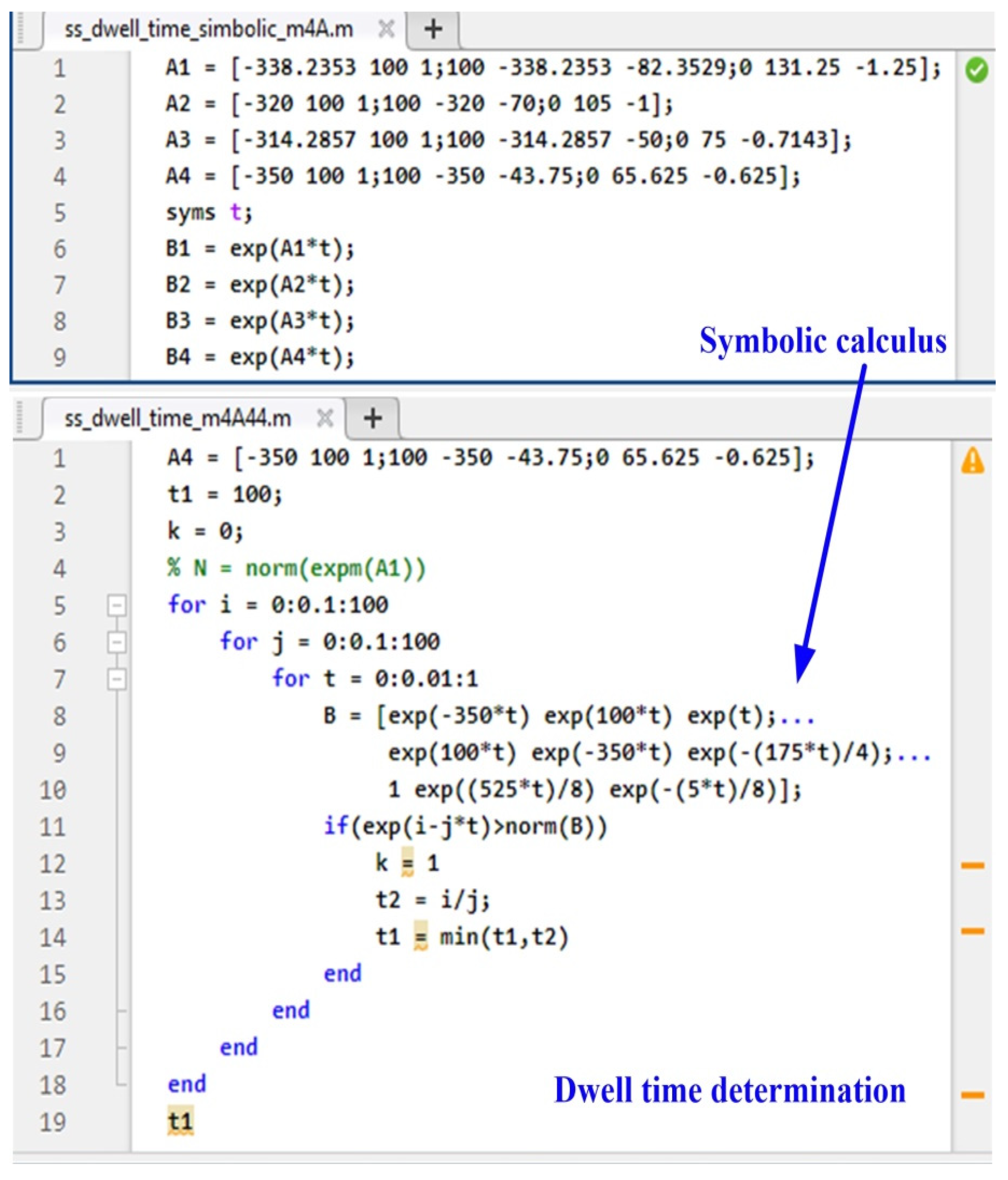
• Matlab program implementation for calculation of the dwell time;
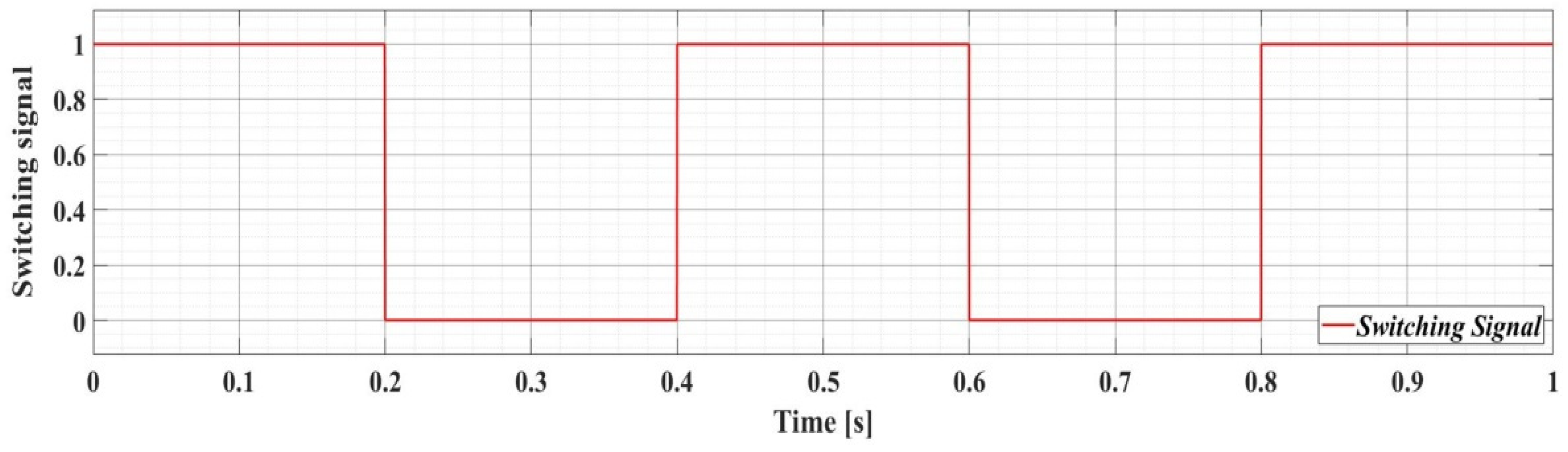
• Numerical simulations development for the PMSM control switched systems using a switching signal with frequency lower than the one corresponding to the dwell time;
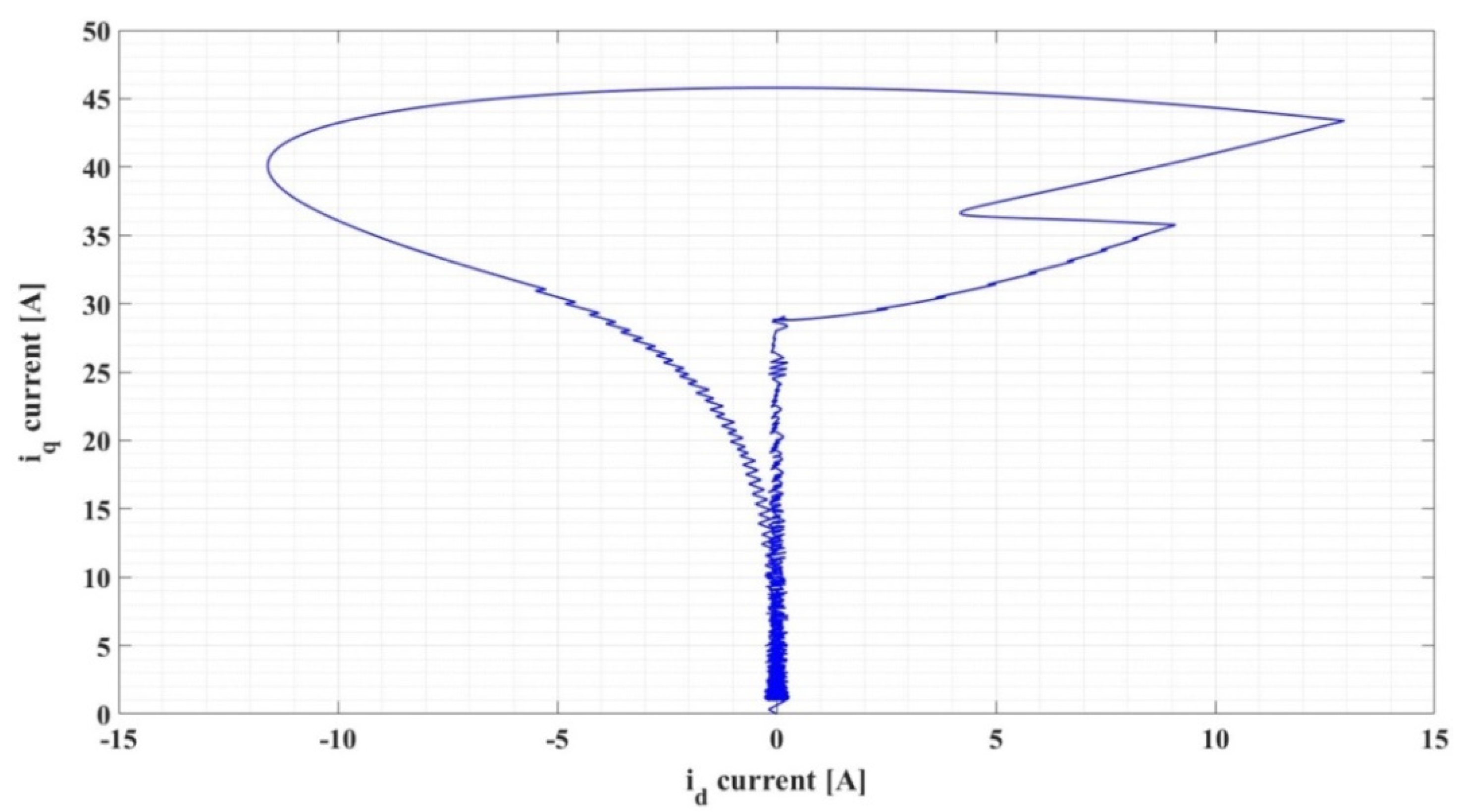
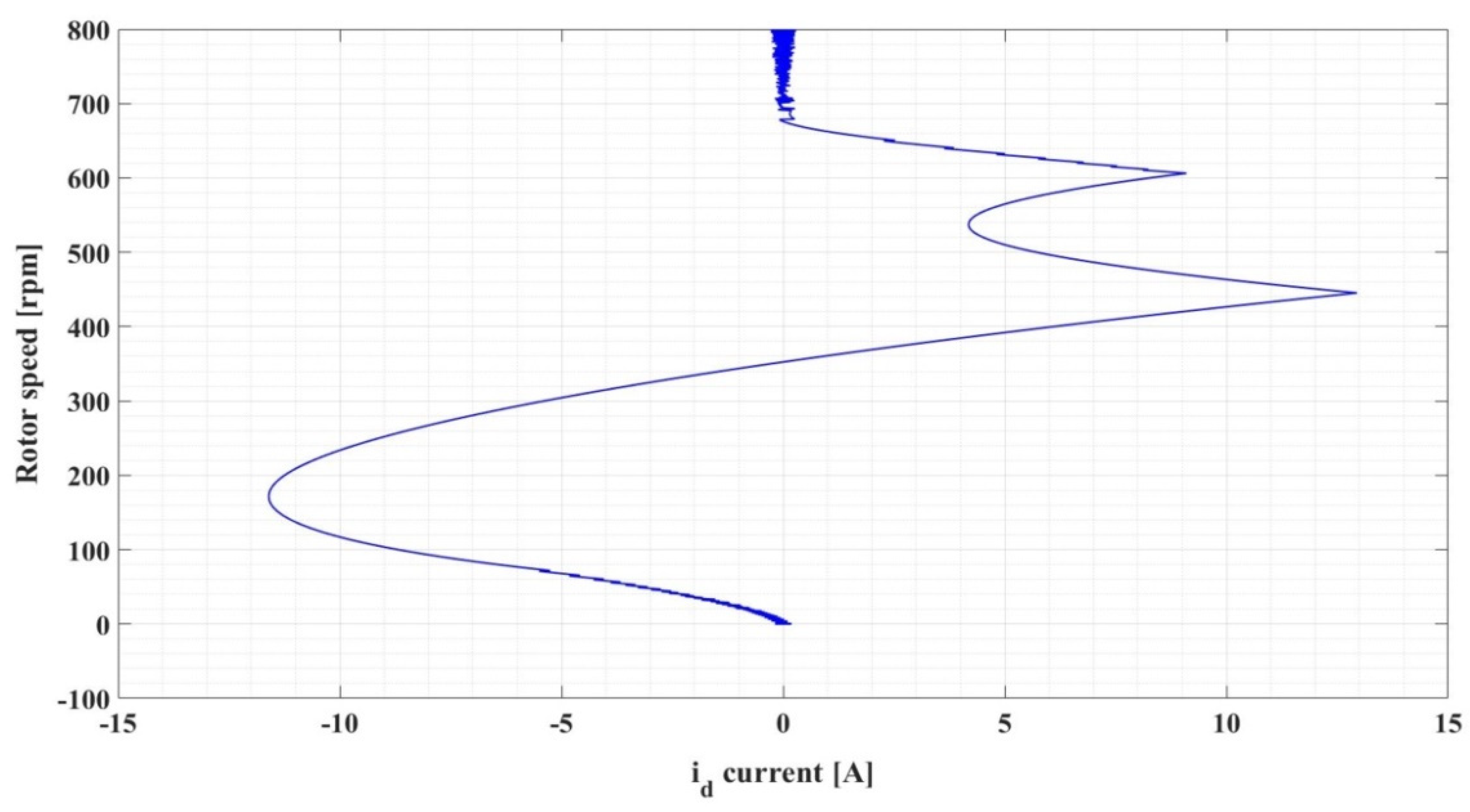
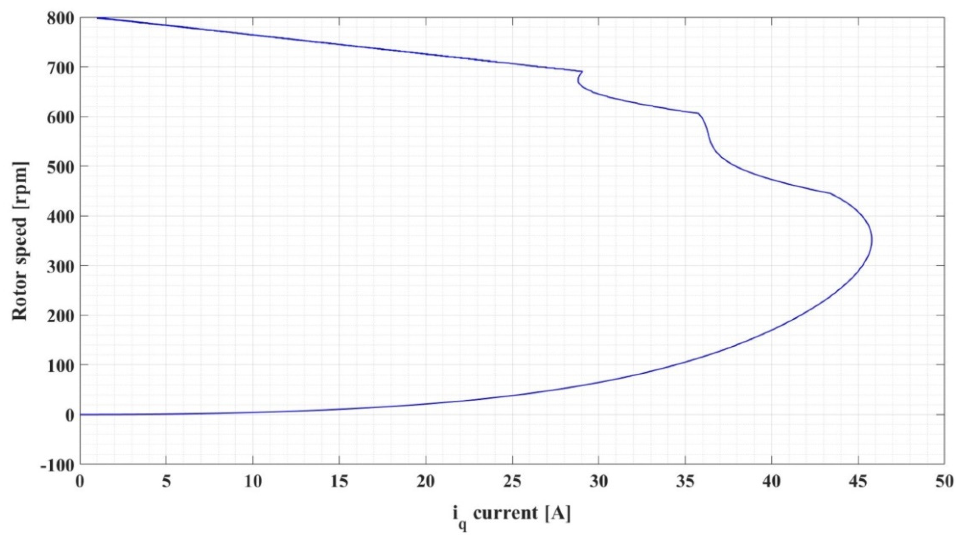
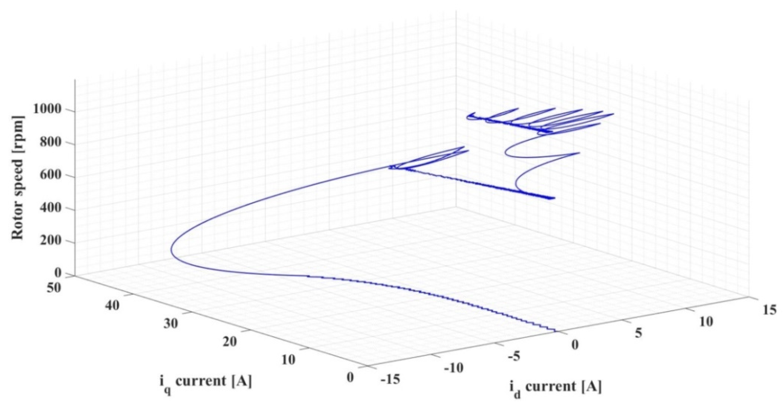
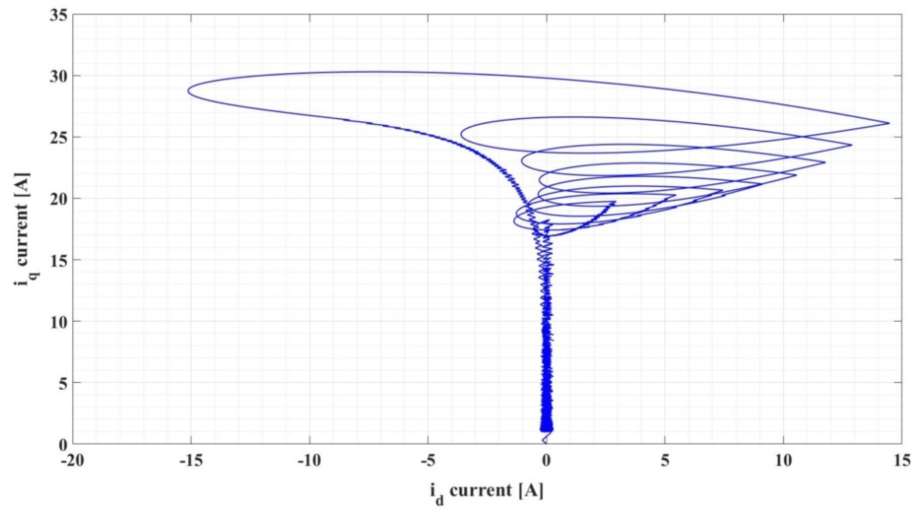
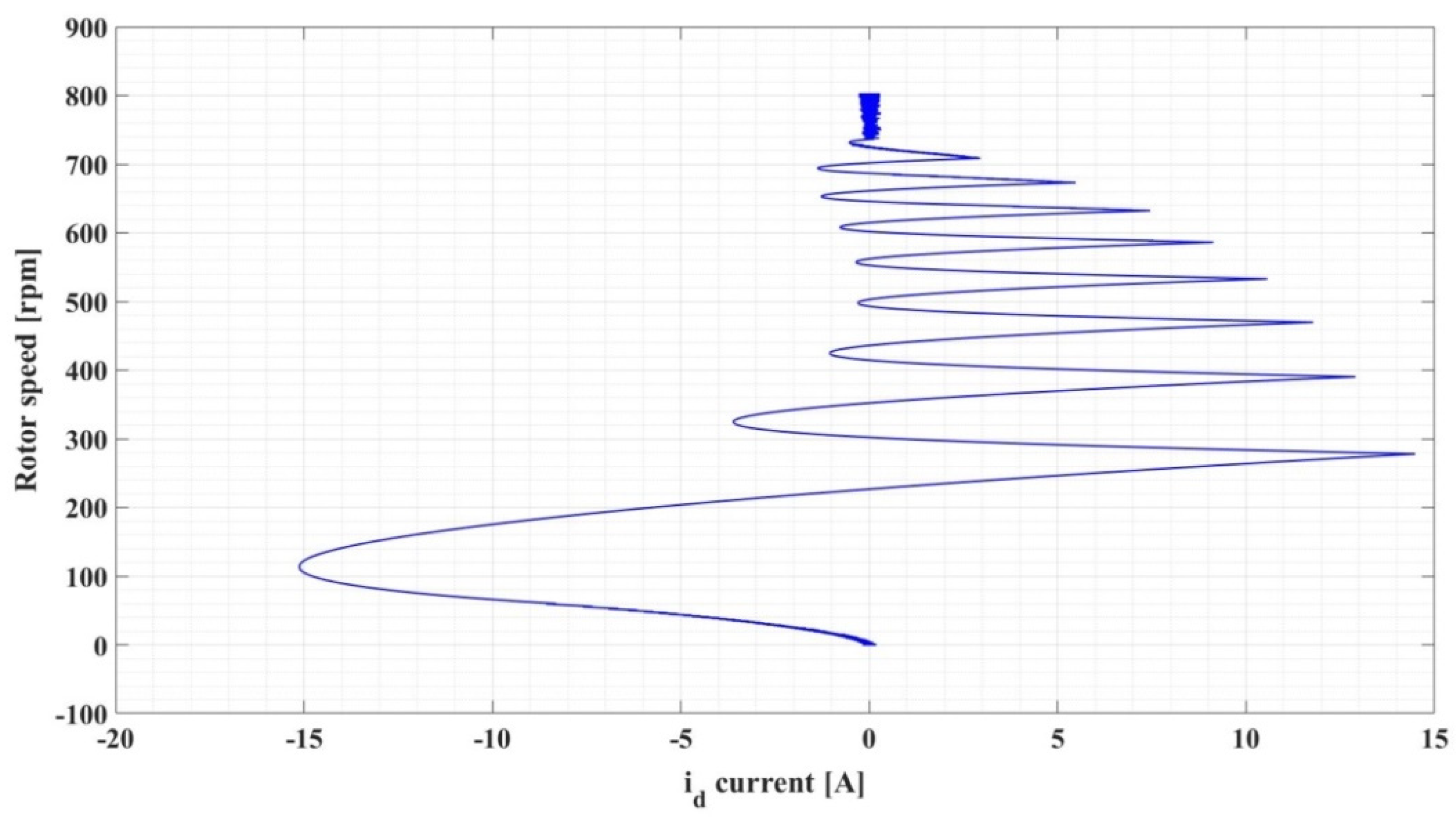
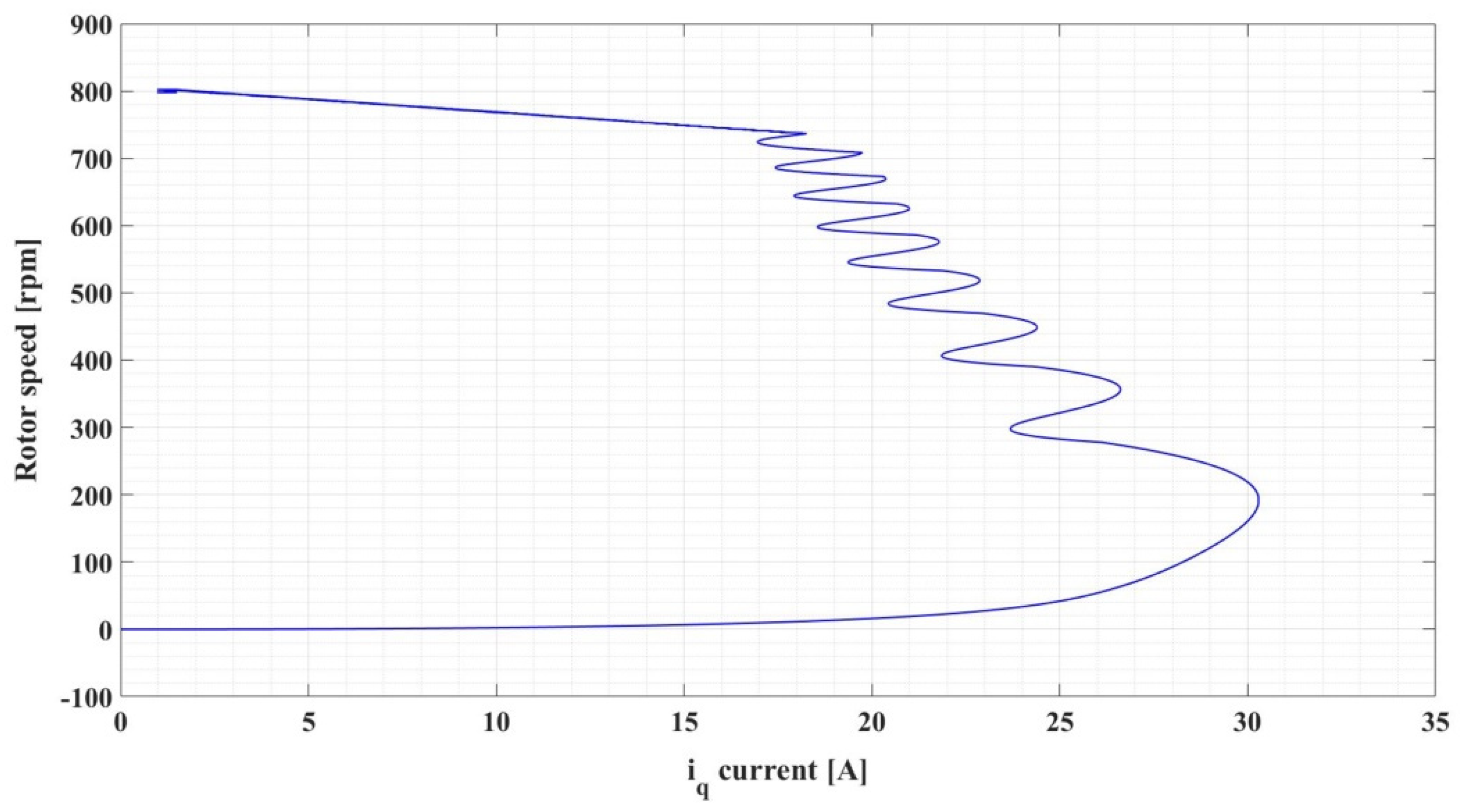
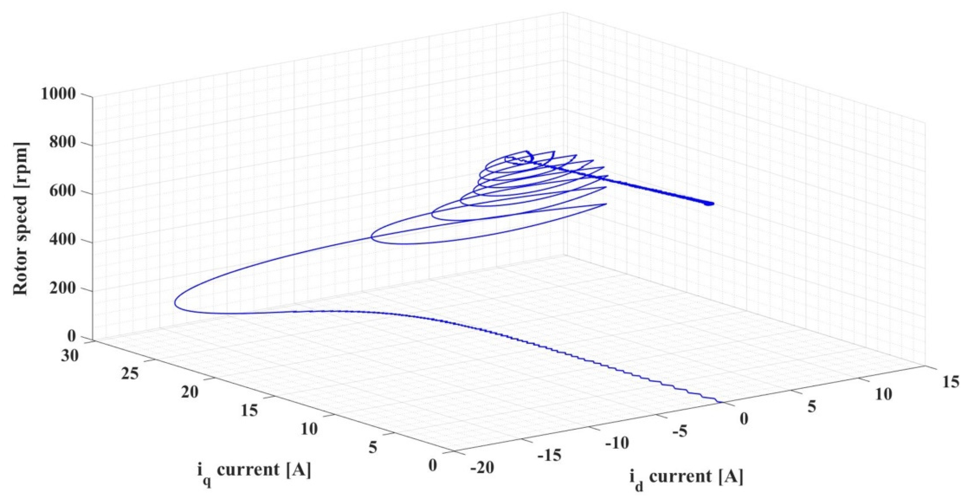
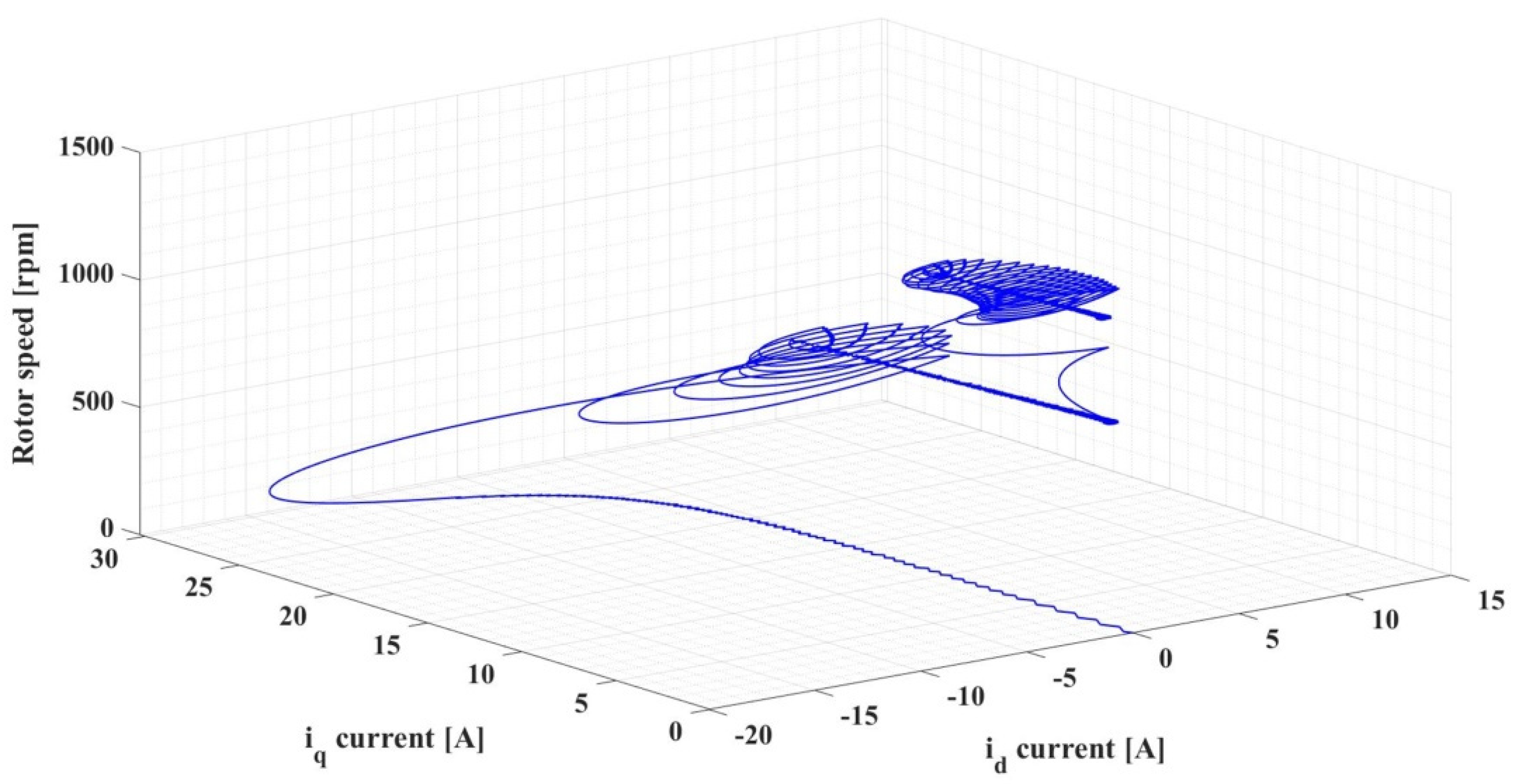
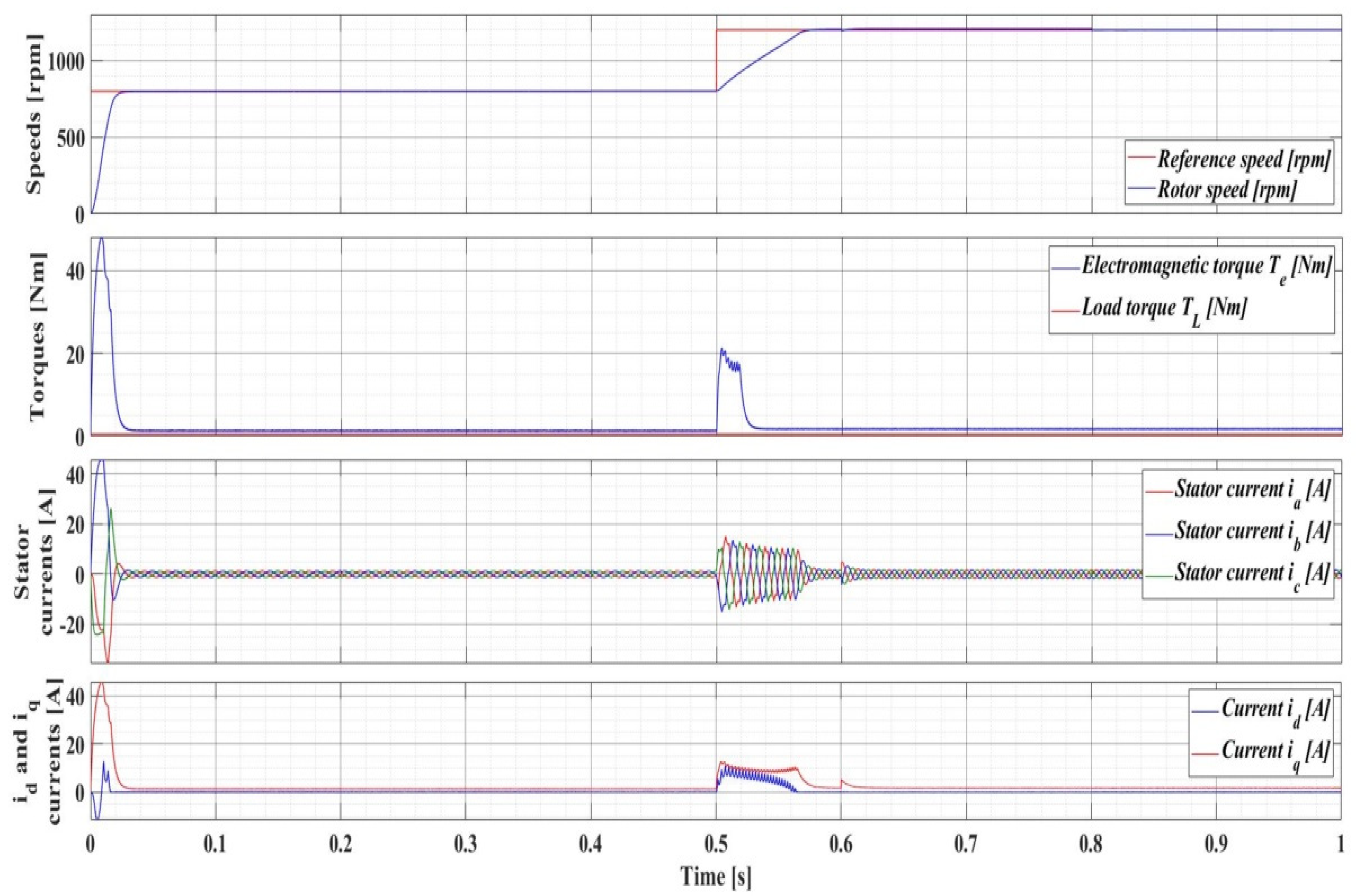
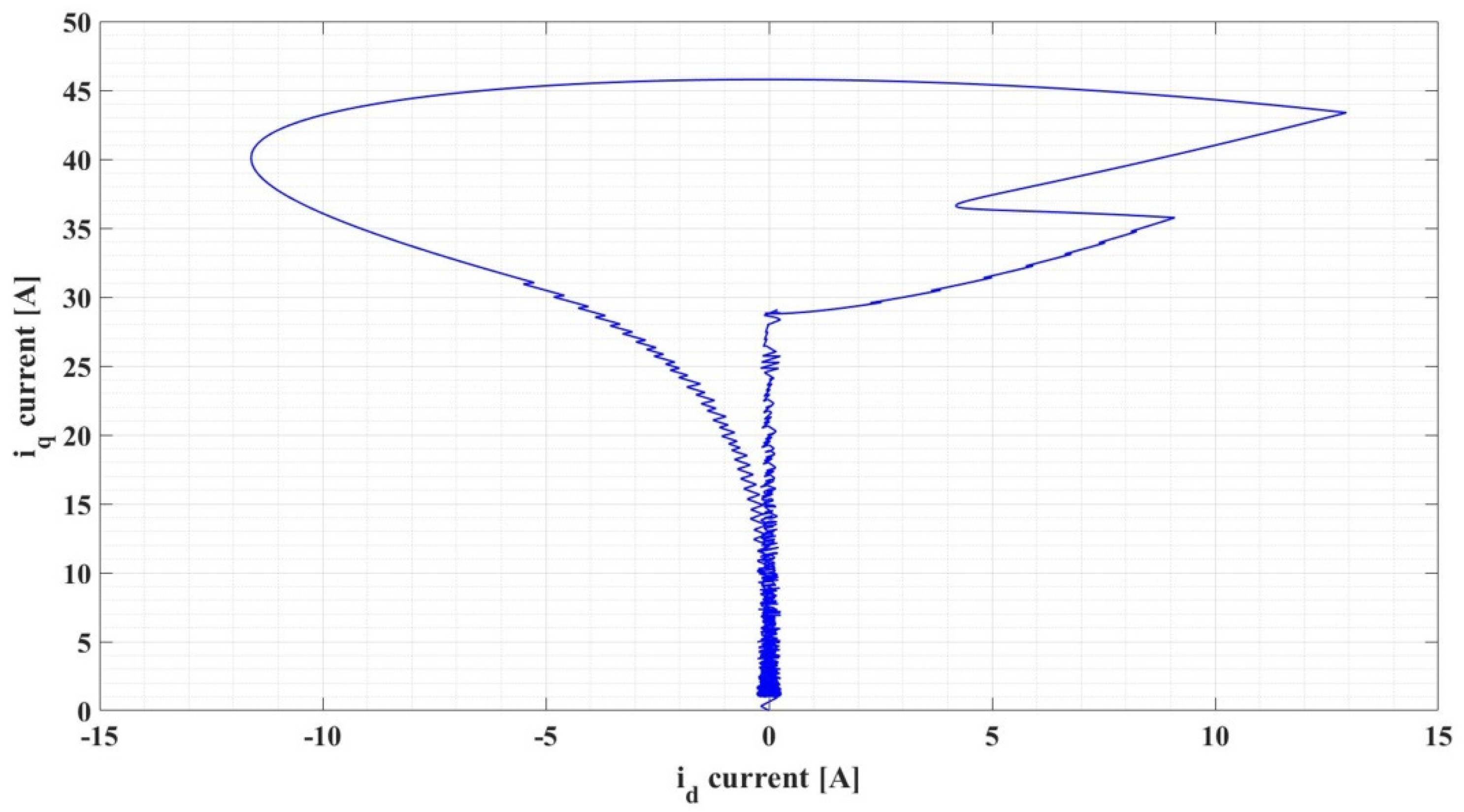
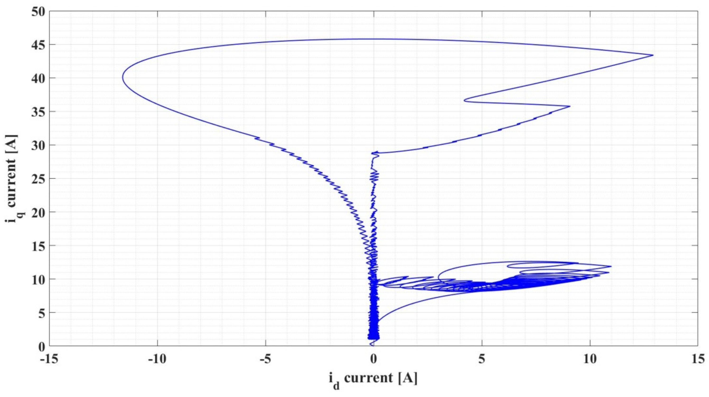
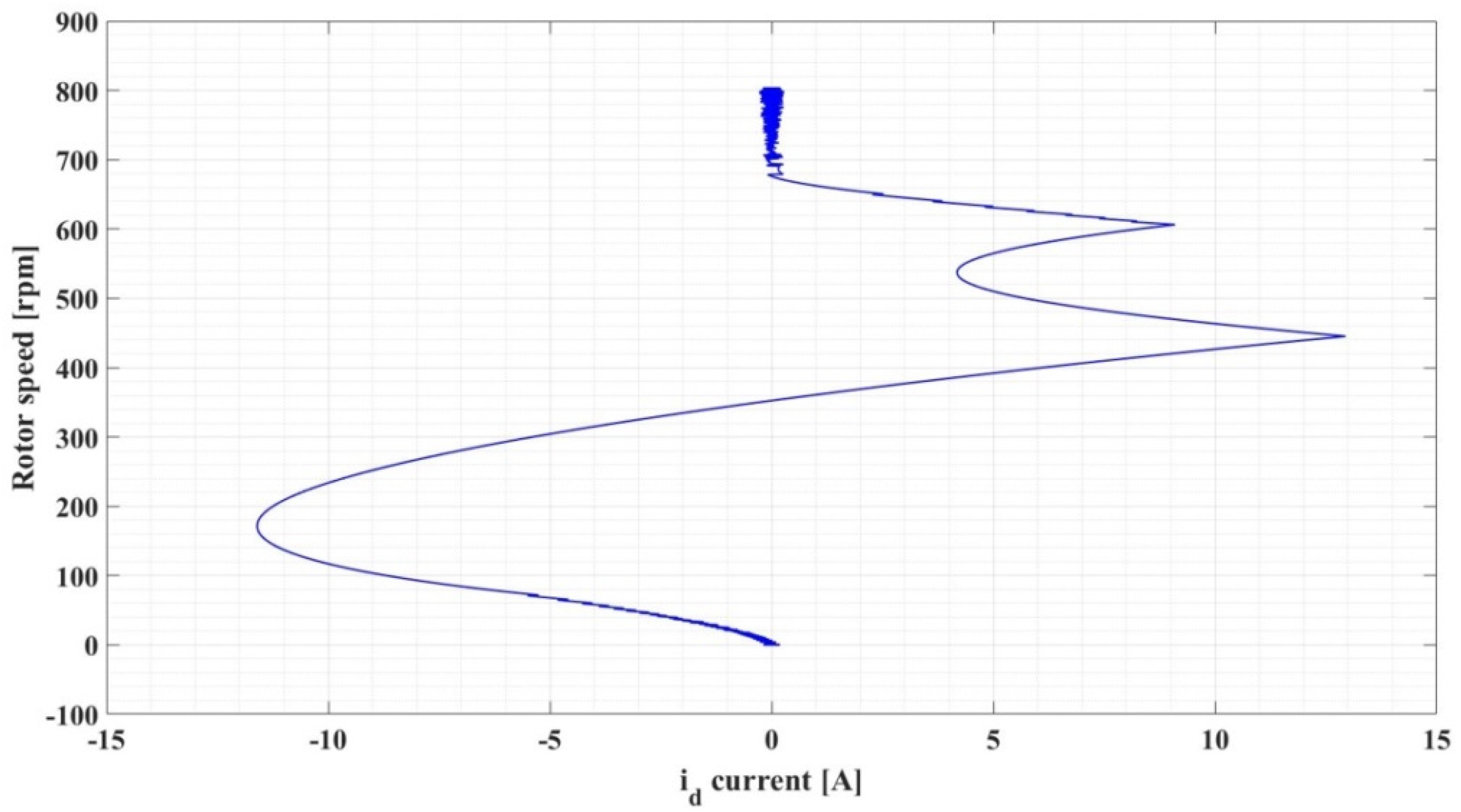
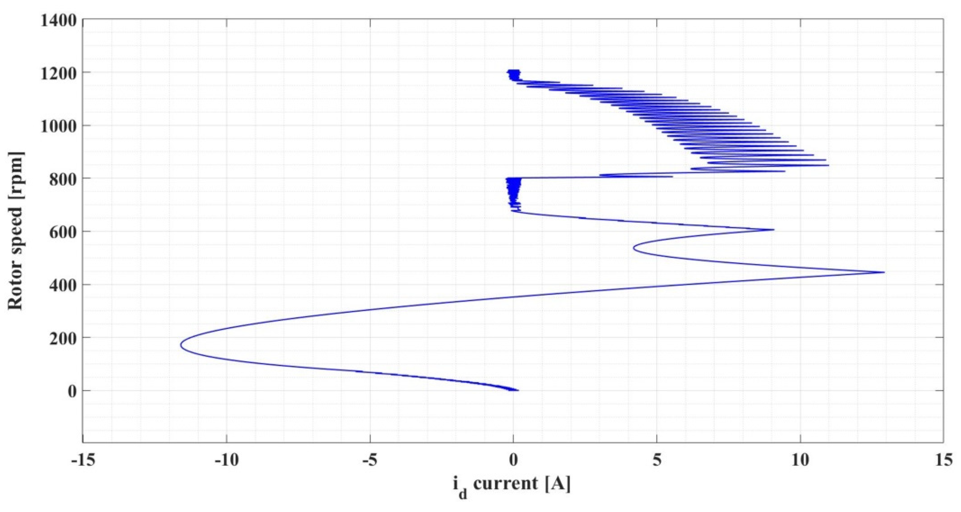
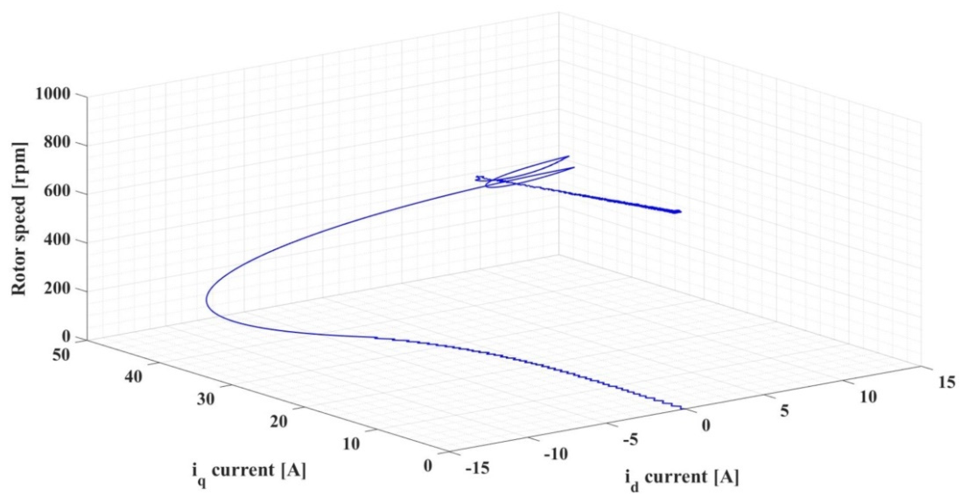
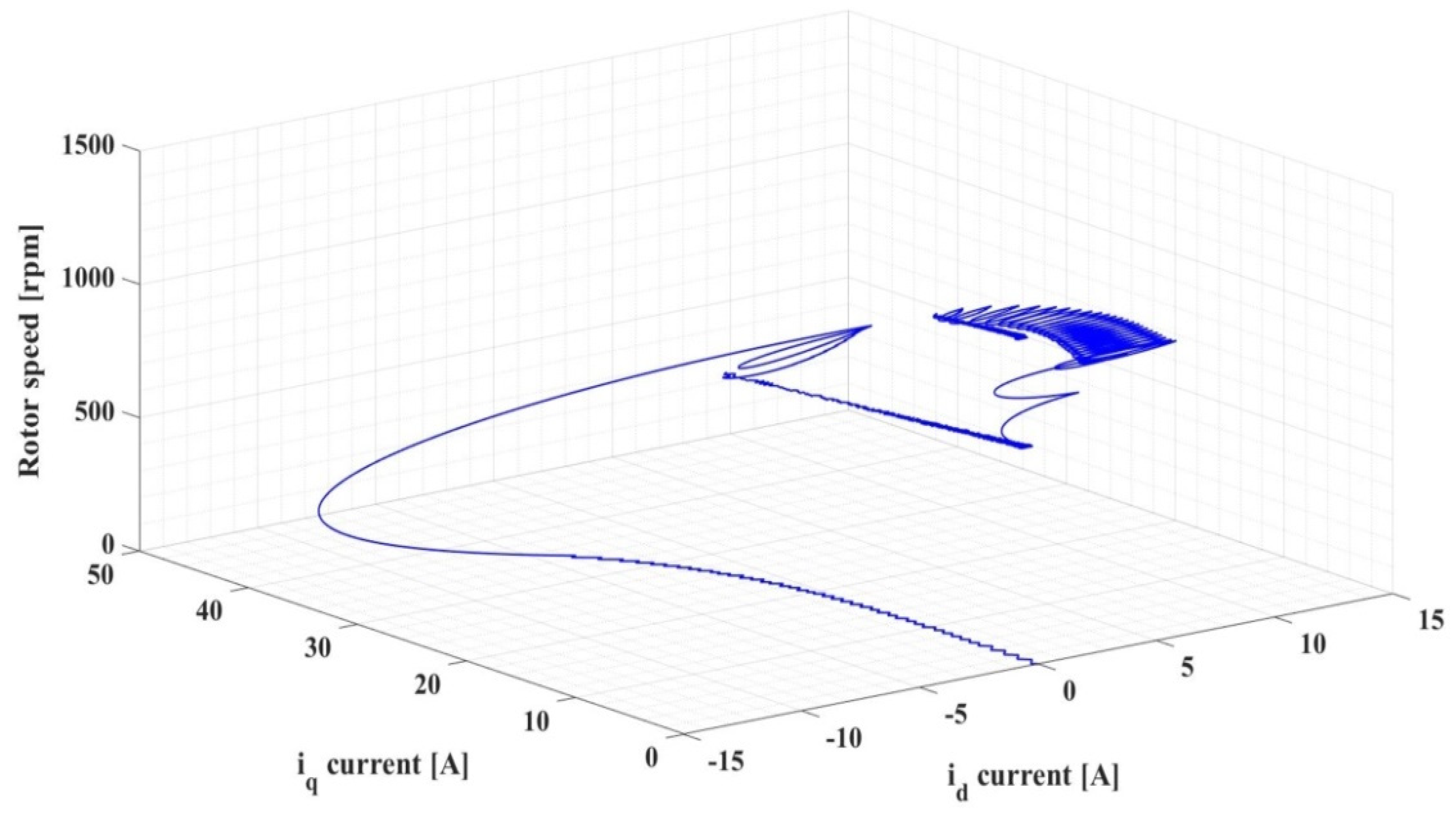
• Qualitative study of the PMSM control system performance by presenting in phase plane and state space the evolution of state vectors: ω PMSM rotor speed, i_q current, and i_d current.

The rest of the paper is organized as follows. The PMSM mathematical model and the FOC-type strategy are presented in Section 2, and the basic concepts of the switched systems are presented in Section 3. The numerical simulations realized in Matlab/Simulink programming and numerical computing environment for the PMSM control switched systems are presented in Section 4, while the final section presents conclusions and perspectives on future approaches.

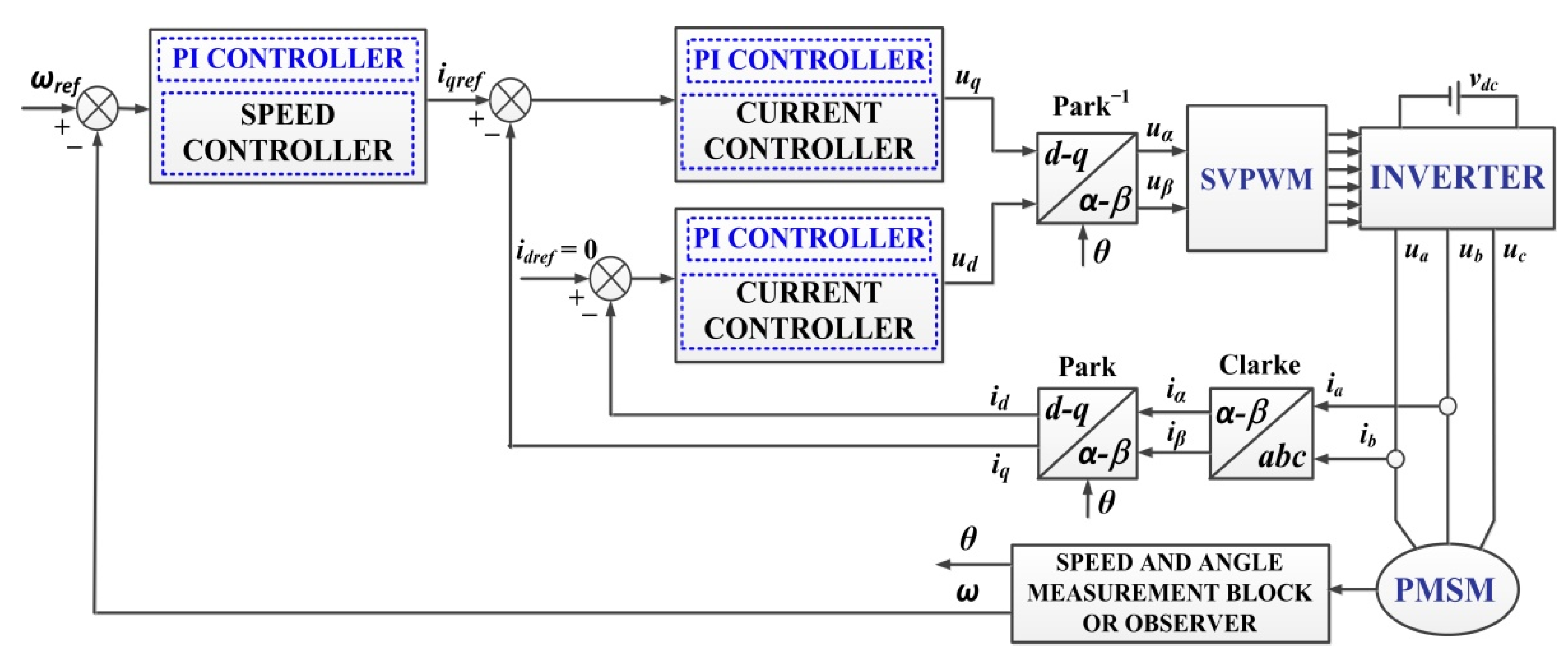
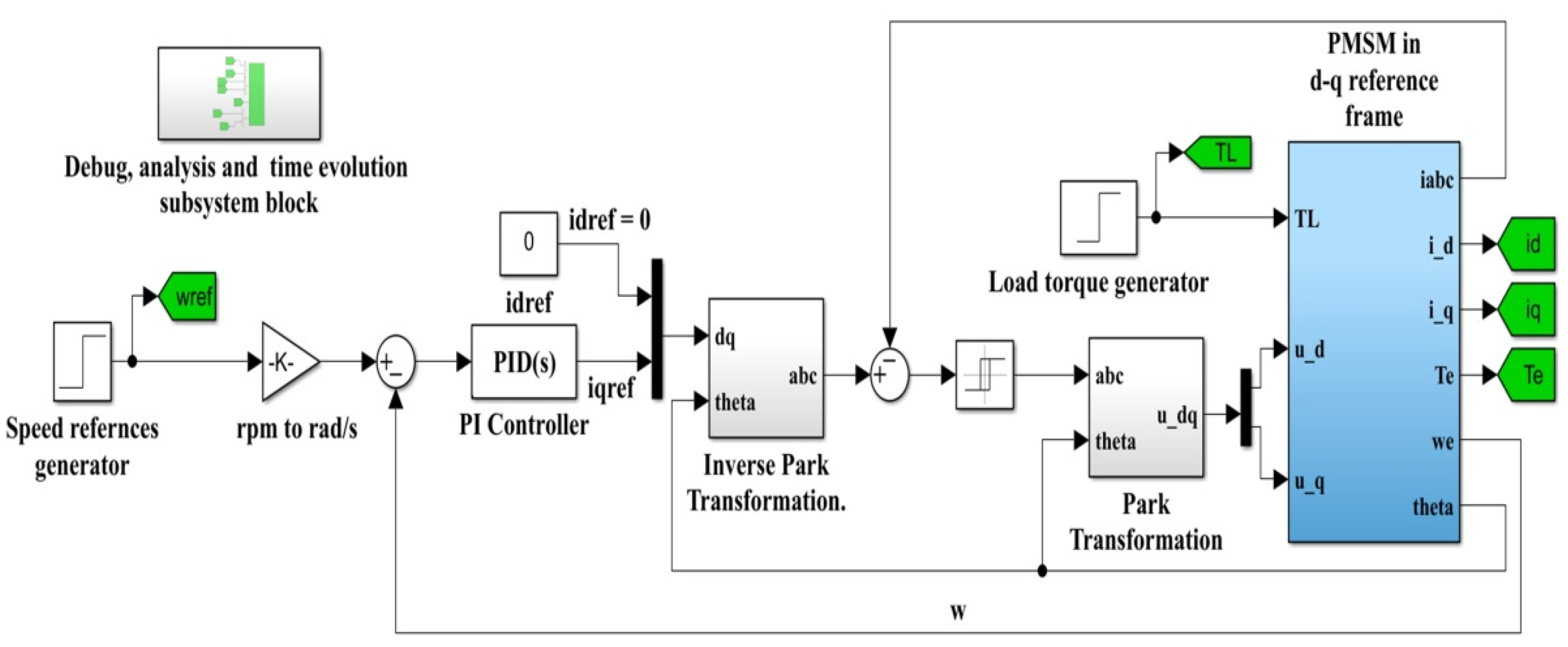
2. PMSM Mathematical Model and FOC-Type Strategy

The FOC–PMSM control strategy shown as a block diagram in Figure 1 emphasizes the two cascade control loops; inner loop for current control and outer loop for the PMSM rotor speed control.

The mathematical model of the PMSM is a nonlinear one, and is presented by the relations in the system (1) [5,6,7,8].

$$\{\begin{array}{l}\frac{d{i}_d}{dt}=-\frac{R_s}{L_d}{i}_d+\frac{L_q}{L_d}{n}_p\omega i_q+\frac{1}{L_d}{u}_d\\ \frac{d{i}_q}{dt}=-\frac{R_s}{L_q}{i}_q-\frac{L_d}{L_q}{n}_p\omega i_d-\frac{{\mathsf{\lambda }}_0}{L_q}{n}_p\omega +\frac{1}{L_q}{u}_q\\ \frac{d\omega }{dt}=\frac{3}{2}\frac{n_p}{J}\left({\mathsf{\lambda }}_0{i}_q+\left(L_d-L_q\right)\hspace{0.17em}{i}_d{i}_q\right)-\frac{1}{J}{T}_L-\frac{B}{J}\omega \\ \frac{d{\theta }_e}{dt}=n_p\omega \end{array}$$

(1)

where u_d, u_q and i_d, i_q denote the stator voltages and stator currents of the PMSM, respectively, these relations being valid in the d–q reference frame. We have denoted the stator inductances and resistances of the PMSM in the d–q reference frame as L_d, L_q and R_d, R_q. We also denoted the stator resistance of the PMSM as R_s, the PMSM rotor speed as ω, the flux linkage as λ₀, the number of pair poles as n_p, the PMSM rotor moment inertia combined with load moment inertia as J, the load torque as T_L, and finally the viscous friction coefficient as B.

For L_d = L_q system (1) can be written under the usual form given by the system (2).

$$\left[\begin{array}{c}{\dot{i}}_d\\ {\dot{i}}_q\\ \dot{\omega }\end{array}\right]=\left[\begin{array}{c}-\frac{R_s}{L_q}{i}_d+n_p\omega \hspace{0.17em}{i}_q\\ -\frac{R_s}{L_q}{i}_q-n_p\omega \hspace{0.17em}{i}_d-\frac{{\mathsf{\lambda }}_0}{L_q}{n}_p\omega \\ \frac{3}{2}\frac{n_p{\mathsf{\lambda }}_0}{J}{i}_q-\frac{B}{J}\omega \end{array}\right]+\left[\begin{array}{cc}\frac{1}{L_q}& 0\\ 0& \frac{1}{L_q}\\ 0& 0\end{array}\right]\left[\begin{array}{c}{u}_d\\ u_q\end{array}\right]+\left[\begin{array}{c}0\\ 0\\ -\frac{T_L}{J}\end{array}\right]$$

(2)

The linearization of the PMSM nonlinear model are achieved around an operating point (x^*, u^*), where the states and commands are given in (3):

$${\underset{\_}{x}}^{*}={\left[\begin{array}{ccc}{i}_d^{*}& i_q^{*}& {\omega }^{*}\end{array}\right]}^T\hspace{0.17em};\hspace{1em}{\underset{\_}{u}}^{*}={\left[\begin{array}{cc}{u}_d^{*}& u_q^{*}\hspace{0.17em}|\hspace{0.17em}{T}_L\end{array}\right]}^T$$

(3)

The following equilibrium relation can be written around this operating point:

$$f\left(x^{*},u^{*}\right)=0$$

(4)

A linear system described in (5) can also be associated with the system (3):

$$\{\begin{array}{c}\dot{x}(t)=\mathit{A}x(t)+\mathit{B}w(t)+\mathit{D}u(t)\\ y(t)=\mathit{C}x(t)\end{array}$$

(5)

where

$$\mathit{A}=\left[\begin{array}{ccc}-\frac{R_s}{L_q}& n_p{\omega }^{*}& n_p{i}_q^{*}\\ n_p{\omega }^{*}& -\frac{R_s}{L_q}& \frac{-n_p{\mathsf{\lambda }}_0}{L_q}\\ 0& \frac{3}{2}\frac{n_p{\mathsf{\lambda }}_0}{J}& -\frac{B}{J}\end{array}\right];\hspace{0.17em}\mathit{B}=\left[\begin{array}{ccc}\frac{1}{L_q}& 0& 0\\ 0& \frac{1}{L_q}& 0\\ 0& 0& -\frac{1}{J}\end{array}\right];\mathit{C}=\left[\begin{array}{ccc}1& 0& 0\\ 0& 0& 1\end{array}\right];\hspace{0.17em}\mathit{D}=\left[\begin{array}{ccc}0& 0& 0\\ 0& 0& 0\end{array}\right]$$

(6)

As a typical example of the static operating point, we can choose a state vector of the PMSM control system defined in the relation (7).

$$\left[\begin{array}{c}{i}_d^{*}\\ i_q^{*}\\ {\omega }^{*}\end{array}\right]=\left[\begin{array}{c}0\\ 1\\ 1200\end{array}\right]$$

(7)

3. Switched Systems—A General Description

Hybrid systems can generally be defined as systems in which continuous and discrete actions and states dynamically interact with each other. Of these systems, those that are continuous, but influenced by discrete events and have the effect of continuously changing the described dynamics, define the switched-type systems. To be define them more accurately, the differential system [22,23,24]

$$\dot{x}(t)=f(x(t))$$

(8)

can be considered, where $f:R^n\to R^n$ is a Lipschitz function.

System (8) can be rewritten in the following form, which characterizes a switched system:

$$\dot{x}(t)=f_{\sigma (t)}(x(t))$$

(9)

where there are N smooth vector fields, $f_i,i\dots N$, and there is also a switching signal piecewise constant $\sigma :\hspace{0.17em}{R}_{+}\to [1,N]$.

For example, the equations defining the temperature pattern in a heated room can be written as [22,23,24]:

$$\{\begin{array}{l}\dot{\theta }(t)=-\mathsf{\lambda }\left(\theta (t)-{\theta }_{ext}(t)\right),\hspace{0.17em}\mathrm{if} \mathrm{the} \mathrm{action} \mathrm{heater} \mathrm{is} \mathrm{off}\\ \dot{\theta }(t)=-\mathsf{\lambda }\left(\theta (t)-{\theta }_{ext}(t)\right)+\beta , \mathrm{if} \mathrm{the} \mathrm{action} \mathrm{heater} \mathrm{is} \mathrm{on}\end{array}$$

(10)

where θ represents the room temperature and λ and β are two quantities which characterize the heating process. Based on these, system (10) can be written as a switched system:

$$\dot{\theta }(t)=-\mathsf{\lambda }\left(\theta (t)-{\theta }_{ext}(t)\right)+\beta \sigma (t),\hspace{0.17em}\hspace{0.17em}\sigma (t)\in \left\{0,1\right\}$$

(11)

For the linear case, the switched systems can be written as

$$\dot{x}(t)=A_{\sigma (t)}x(t),\hspace{0.17em}\hspace{0.17em}x(0)=x_0$$

(12)

A necessary condition for the stability of the switching system where the switching random function $\sigma (t)=i,\hspace{0.17em}\forall t$ is that all matrices $A_i,i=1,\dots ,N$ are Hurwitz.

If σ(t) is a switching signal defined for example as in the following expression:

$$\sigma (t)=\{\begin{array}{l}2,\hspace{1em}t\in [0,T)\\ 1\hspace{1em}t\in [T,2T)\end{array}$$

(13)

where 2T is the period of the system, and $\Phi (t,\tau )$ is the transition matrix of the system (12) considered periodic in this example, the monodromy matrix is defined as

$$\Phi (2T,0)=e^{A{T}_2}{e}^{A_{1}T}$$

(14)

According to [23] the system is asymptotically stable if the monodromy matrix has subunit eigenvalues modulus.

For the general form of the linear case, one can consider the switched systems

$$\{\begin{array}{l}\dot{x}(t)=A_{\sigma (t)}x(t)+B_{\sigma (t)}u(t)\\ y(t)=C_{\sigma (t)}x(t)+D_{\sigma (t)}u(t)\end{array}$$

(15)

where the notations are the usual ones, and $A_i,i=1,\dots ,N$, are Hurwitz matrices.

There is the matter of finding the minimum of $\gamma >0$ for which

$$\underset{w\in L_2(0,\infty )}{\sup }\frac{{\Vert y\Vert }_2}{{\Vert w\Vert }_2}<\gamma$$

(16)

and $\gamma$ fulfills the condition

$$\gamma \ge \underset{i}{\max }\left\{{\gamma }_i\right\}$$

(17)

where: ${\gamma }_i$ is the $H_{\infty }$ norm associated with the system $\left(A_i,B_i,C_i,D_i\right)$ defined in relation (16).

In this respect the following theorem is presented [24,25,26]:

Theorem 1.

Given the system (15) and assuming that there is a positive definite matrix P so that the following relation is satisfied,

$$\left[\begin{array}{ccc}{A}_i^{T}P+P{B}_i& P{B}_i& C_i^T\\ B_i^{T}P& -{\gamma }^{2}I& D_i^T\\ C_i& D_i& -I\end{array}\right]<0,\hspace{0.17em}\forall i\in N$$

(18)

then the global asymptotic stability of the switched systems (15) is ensured for the switching signal $\sigma$ and in addition the following inequality is fulfilled:

$$\underset{w\in L_2,\hspace{0.17em}w\ne 0}{\sup }{\displaystyle \underset{0}{\overset{\infty }{\int }}\left(y^{T}y-{\gamma }^2{w}^{T}w\right)dt<0}$$

(19)

Proof of Theorem 1.

From Schur’s lemma and from (18), the inequality ${\gamma }^{2}I-D_i^T{D}_i>0$ and the relation (20) are obtained.

$$A_i^{T}P+P{A}_i+\left(P{B}_i+C_i^T{D}_i\right){\left({\gamma }^{2}I-D_i^T{D}_i\right)}^{-1}{\left(P{B}_i+C_i^T{D}_i\right)}^T+C_i^T{C}_i<0,\hspace{0.17em}\forall i$$

(20)

Based on these, relation (21) ensures the global asymptotic stability in the case of random switching for any input w square-integrable.

$$A_i^{T}P+P{A}_i<0$$

(21)

This is equivalent to choosing a Lyapunov function $V(x)=x^{T}Px$ whose derivative $\dot{V}<0$.

$$w^{*}={\left({\gamma }^{2}I-D_i^T{D}_i\right)}^{-1}{\left(P_i{B}_i+C_i^T{D}_i\right)}^{T}x$$

(22)

Based on notation (22), the next relation is obtained:

$$\begin{array}{l}\dot{V}(x)=x^T\left(A_{\sigma }^{T}P+P{A}_{\sigma }\right)x+2x^{T}P{B}_{\sigma }w<\\ \hspace{0.17em}\hspace{0.17em}\hspace{0.17em}\hspace{0.17em}\hspace{0.17em}\hspace{0.17em}\hspace{0.17em}<-y^{T}y+{\gamma }^{-2}{w}^{T}w-{\left(w-w^{*}\right)}^T\left({\gamma }^{2}I-D_i^T{D}_i\right)\left(w-w^{*}\right)\\ \hspace{0.17em}\hspace{0.17em}\hspace{0.17em}\hspace{0.17em}\hspace{0.17em}\hspace{0.17em}\hspace{0.17em}<-y^{T}y+{\gamma }^{-2}{w}^{T}w\end{array}$$

(23)

and from this, by integrating $\dot{V}$, the relation (24) is obtained, which represents the conclusion of the proof of the theorem.

$${\displaystyle \underset{0}{\overset{\infty }{\int }}\left(y^{T}y-{\gamma }^2{w}^{T}w\right)dt<0},\hspace{0.17em}\forall \sigma ,\hspace{0.17em}\forall w\ne 0,\hspace{0.17em}w\in L_2$$

(24)

Let us consider ${\alpha }_i,i=1,\dots ,N$, a simplex, i.e., ${\alpha }_i\ge 0$ and ${\displaystyle \sum _{i=1}^N{\alpha }_i}=1$, and using the relation (18) accordingly, by applying Schur’s lemma we obtain the relation (20) in condensed form (25):

$$A_{\alpha }^{T}P+P{A}_{\alpha }+\left(P{B}_{\alpha }+C_{\alpha }^T{D}_{\alpha }\right){\left({\gamma }^{2}I-D_{\alpha }^T{D}_{\alpha }\right)}^{-1}{\left(P{B}_{\alpha }+C_{\alpha }^T{D}_{\alpha }\right)}^T+C_{\alpha }^T{C}_{\alpha }<0$$

(25)

where

$$A_{\alpha }={\displaystyle \sum _{i=1}^N{\alpha }_i{A}_i},\hspace{1em}{B}_{\alpha }={\displaystyle \sum _{i=1}^N{\alpha }_i{B}_i},\hspace{1em}{C}_{\alpha }={\displaystyle \sum _{i=1}^N{\alpha }_i{C}_i},\hspace{1em}{D}_{\alpha }={\displaystyle \sum _{i=1}^N{\alpha }_i{D}_i}$$

(26)

Under these conditions, norm $H_{\infty }$ of the system $\left(A_{\alpha },B_{\alpha },C_{\alpha },D_{\alpha }\right)$ is less than $\gamma$ for any α in the considered simplex.

The following are two examples that ensure a better understanding of what has been presented so far and of how the presentation continues.

3.1. Example 1

Let us consider a switching system described by the following subsystems defined by the matrices:

$$A_1=\left[\begin{array}{cc}-3& 1\\ 0& -1\end{array}\right],\hspace{1em}{A}_2=\left[\begin{array}{cc}-2& 1\\ 0& -5\end{array}\right]$$

(27)

Using the Matlab environment, the eigenvalues are calculated as follows: eig(A₁) = {−3, −1} and eig(A₂) = {−2, −5}. The result is that A₁ and A₂ are Hurwitz matrices. By applying the relation (21), we obtain the next system:

$$\{\begin{array}{l}{A}_1^{T}P+P{A}_1<0\\ A_2^{T}P+P{A}_2<0\end{array}$$

(28)

Using the Matlab environment and YALMIP toolbox, the matrix P containing the solution to the system (28) is obtained as:

$$P=\left[\begin{array}{cc}0.2849& 0.0359\\ 0.0359& 0.1821\end{array}\right]$$

(29)

Since eig(P) = {0.1708, 0.2969}, matrix P is positive definite and ensures the global asymptotic stability of the switched systems defined by (27).

3.2. Example 2

Let us consider a switching system described by the following subsystems defined by the matrices:

$$A_1=\left[\begin{array}{cc}-1& -1\\ 1& -1\end{array}\right],\hspace{1em}{A}_2=\left[\begin{array}{cc}-1& -10\\ 0.1& -1\end{array}\right]$$

(30)

Using the Matlab environment, the eigenvalues are calculated as eig(A₁) = eig(A₂) = {−1.0000 + 1.0000i, −1.0000 − 1.0000i} from which it results that A₁ and A₂ are Hurwitz matrices.

Following the above method, it is demonstrated that there is no matrix P > 0 which verifies the system (28). Thus, the above theorem cannot be applied and it cannot be stated that the switched system described by (30) is stable even if the two subsystems are stable. This proves once again that local stability does not imply global stability, and the conditions imposed by a system such as (28) are too restrictive. In contrast, Theorem 2, below, has more restrictive conditions but ensures the stability of the switched systems [24].

First, the term dwell time is described by the following definition [25,26,27]:

Definition 1.

If$T>0,\hspace{0.17em}T\in R$so that

$$\underset{q}{\inf }\left(t_q-t_{q-1}\right)\ge T$$

(31)

then T is called dwell time of the switched systems.

Theorem 2.

Assume that for $T>0$there is a set of positive definite matrices$\left\{P_1,\dots ,P_N\right\}$of corresponding dimensions, so as to fulfill the inequalities:

$$A_i^T{P}_i+P_i{A}_i<0,\hspace{1em}\forall i\in \left\{1,\dots ,N\right\}$$

(32)

$$e^{A_i^{T}T}{P}_j{e}^{A_{i}T}-P_j<0,\hspace{1em}\forall i\ne j,\hspace{1em}i,j\in \left\{1,\dots ,N\right\}$$

(33)

Under these conditions, the time switching control law $\sigma (t)=i\in \left\{1,\dots ,N\right\},\hspace{1em}t\in \left[t_k,t_{k+1}\right)$ where t_k and t_k+1 are successive switching moments so that $t_{k+1}-t_k\ge T,\hspace{0.17em}\forall k\in \mathit{N}$ ensures the global asymptotic stability of the switched system.

Proof of Theorem 2.

A draft of the demonstration consists in the fact that by choosing a Lyapunov function

$$\dot{V}(x(t))=x{(t)}^T{P}_{\sigma (t)}x(t)$$

(34)

and calculating its derivative, the next relation is obtained:

$$\dot{V}(x(t))=x{(t)}^T\left(A_i^T{P}_i+P_i{A}_i\right)x(t)<0$$

(35)

From this, α > 0 and β > 0 so that

$${\Vert x(t)\Vert }^2\le \beta e^{-\alpha (t-t_k)}V(x(t_k)),\hspace{0.17em}\forall t\in \left[t_k,t_{k+1}\right)$$

(36)

By exploiting the relation (33) the next form can be obtained:

$$\begin{array}{l}\dot{V}(x(t_{k+1}))=x{(t_{k+1})}^T{P}_{j}x(t_{k+1})=x{(t_k)}^T{e}^{A_i^T{T}_k}{P}_j{e}^{A_i{T}_k}x(t_k)\\ \hspace{0.17em}\hspace{0.17em}\hspace{0.17em}\hspace{0.17em}\hspace{0.17em}\hspace{0.17em}\hspace{0.17em}\hspace{0.17em}\hspace{0.17em}\hspace{0.17em}\hspace{0.17em}\hspace{0.17em}\hspace{0.17em}\hspace{0.17em}\hspace{0.17em}<x{(t_k)}^T{e}^{A_i^T(T_k-T)}{P}_i{e}^{A_i(T_k-T)}x(t_k)\\ \hspace{0.17em}\hspace{0.17em}\hspace{0.17em}\hspace{0.17em}\hspace{0.17em}\hspace{0.17em}\hspace{0.17em}\hspace{0.17em}\hspace{0.17em}\hspace{0.17em}\hspace{0.17em}\hspace{0.17em}\hspace{0.17em}\hspace{0.17em}\hspace{0.17em}<x{(t_k)}^T{P}_{i}x(t_k)\\ \hspace{0.17em}\hspace{0.17em}\hspace{0.17em}\hspace{0.17em}\hspace{0.17em}\hspace{0.17em}\hspace{0.17em}\hspace{0.17em}\hspace{0.17em}\hspace{0.17em}\hspace{0.17em}\hspace{0.17em}\hspace{0.17em}\hspace{0.17em}\hspace{0.17em}<V(x(t_k))\end{array}$$

(37)

This results in $\mu \in (0,1)$ so that

$$V(x(t_k))\le {\mu }^{k}V(x_0),\hspace{0.17em}\forall k\in \mathit{N}$$

(38)

From relations (36) and (38) the global asymptotic stability of the switched system is obtained. It can be pointed out that inequalities (32) and (33) are known as Lyapunov–Metzler inequalities.

A number of ways of estimating the dwell time of the switched systems are presented in [26,27], where we propose an estimate used in practical examples. An upper limit for the minimum dwell time T* is given by T* $T^{*}\le \underset{i=1,\dots ,N}{\max }\left\{T_i\right\}$, where

$$T_i=\underset{\alpha >0,\beta >0}{\inf }\left\{\frac{\alpha }{\beta }:\Vert e^{A_{i}t}\Vert <e^{\left(\alpha -\beta t\right)},\hspace{0.17em}\forall t\ge 0\right\}$$

(39)

Evidently, by using the above theorems, the stability of a switched system can be demonstrated if the switching signal does not switch more often than the dwell time. In terms of establishing a control law of a switched system, similarly to the way the above Lyapunov functions have been chosen, corresponding control laws can be obtained for the closed loop system.

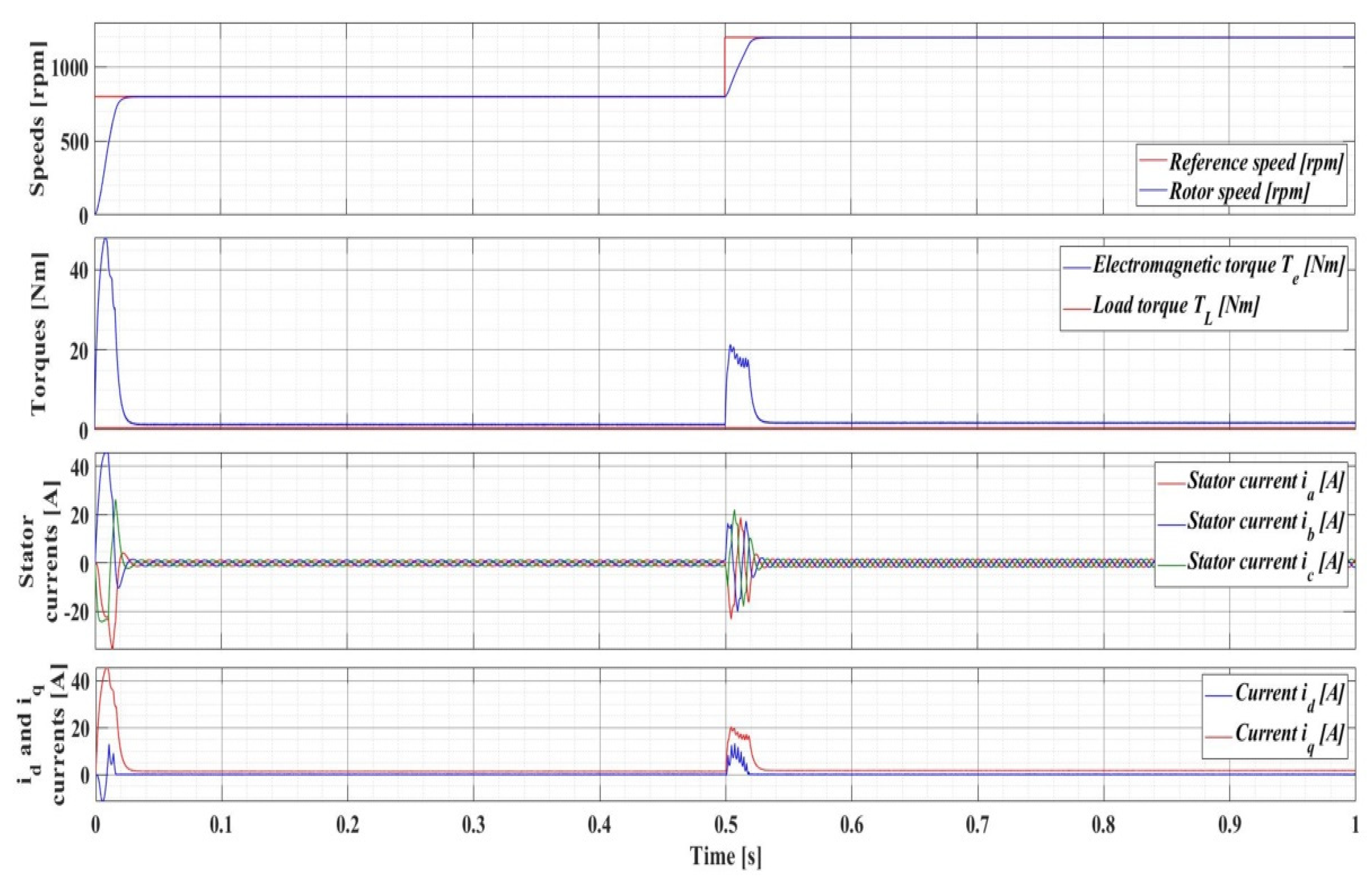
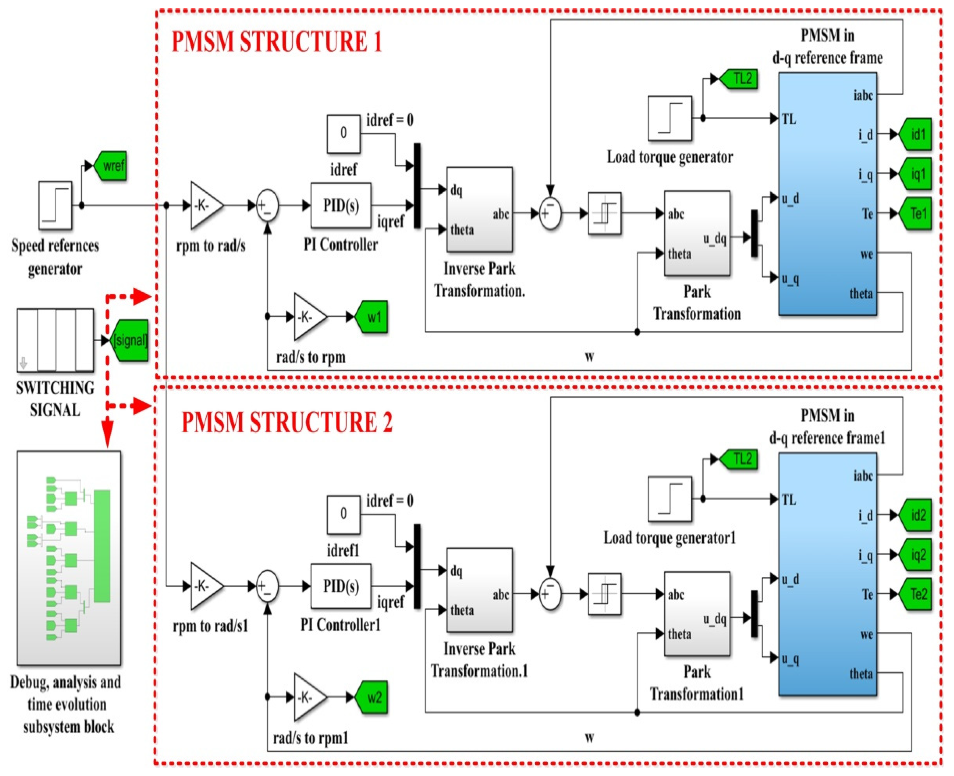
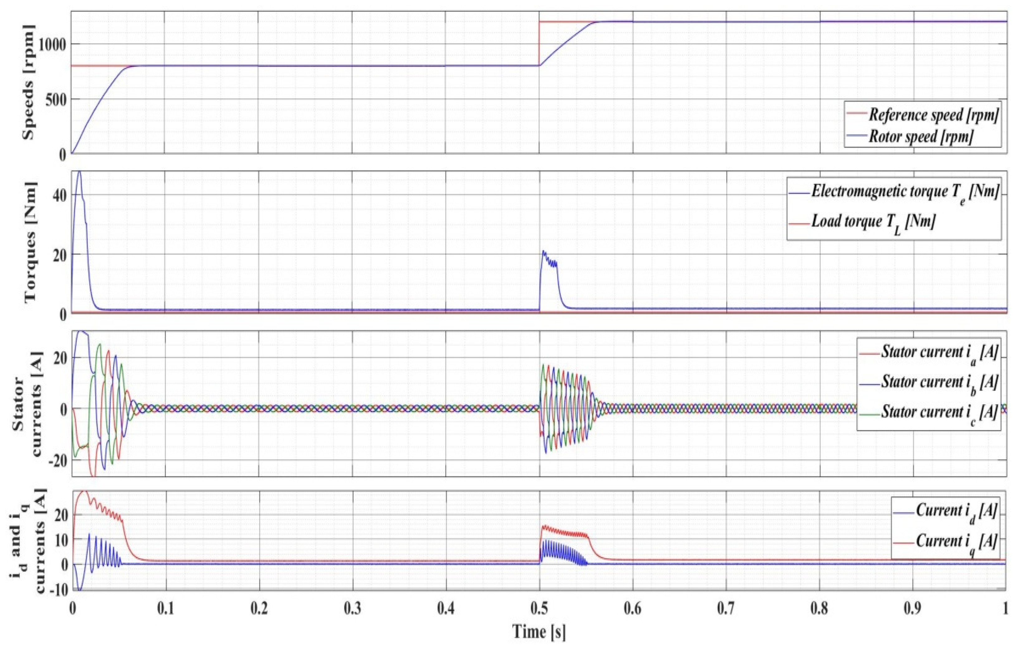
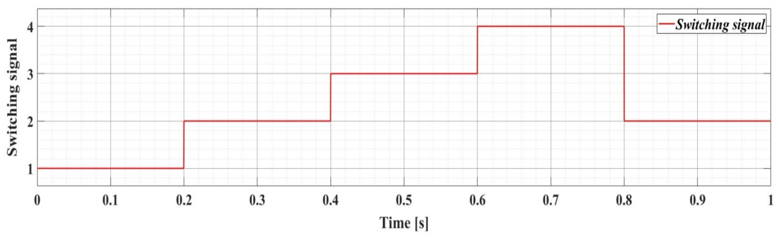
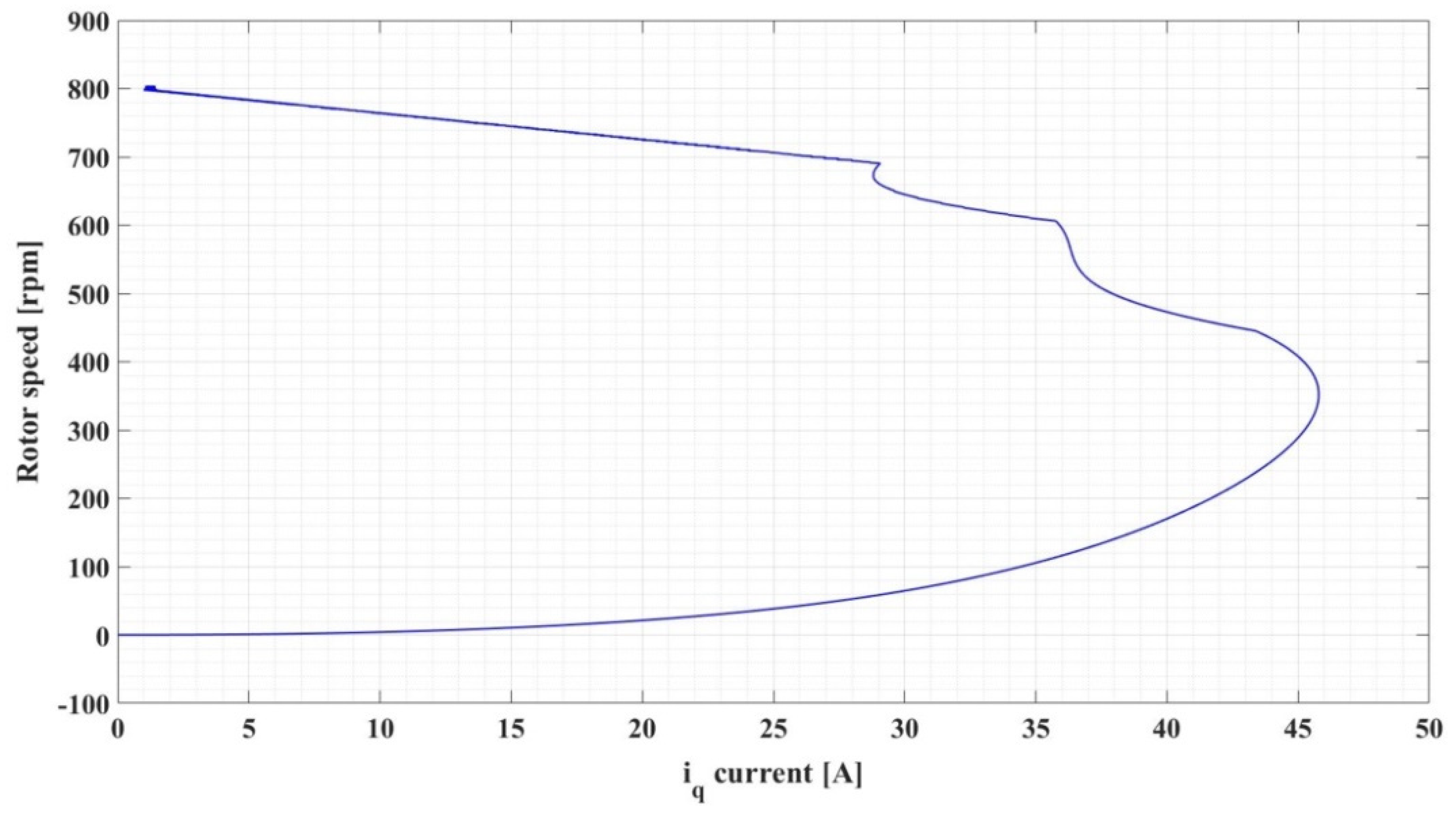
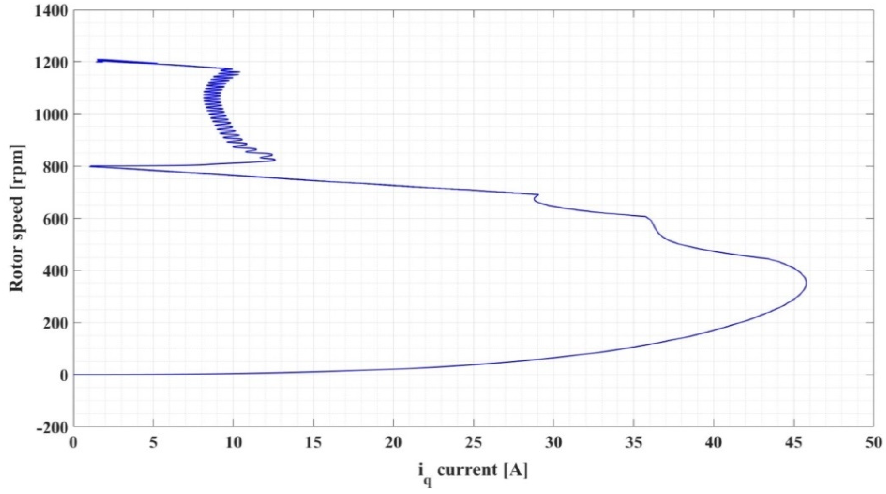
4. Numerical Simulations for PMSM Control Switched Systems

For the PMSM control in the classical structure (Figure 1), the so-called FOC control strategy, with the outer speed control loop supplying the references for the inner i_d and i_q current control loops, Figure 2 shows the implementation in Matlab/Simulink, noting that the current reference i_dref is set to 0 for the maximization of the electromagnetic torque T_e.

Usually, the controllers of the two inner current control loops and the controller of the outer PMSM rotor speed control loop are of PI type.

Below the numerical simulations are presented for the control system of a PMSM, with nominal parameters as given in

Table 1. PMSM nominal parameters.

Parameter	Value	Unit
Stator resistance—Rs	2.875	Ω
Inductances on d-q axis—Ld, Lq	0.0085	H
Combined inertia of PMSM rotor and load—J	0.008	kg·m2
Combined viscous friction of PMSM rotor and load—B	0.01	N·m·s/rad
Flux induced by the permanent magnets of the PMSM rotor in the stator phases—λ0	0.175	Wb
Pole pairs number—np	4	−

.

Figure 3 shows the evolution of the parameters of interest (rotor speed noted with ω, electromagnetic and load torques noted with T_e and T_L, stator currents noted with i_a, i_b, i_c, and d-q frame currents noted with i_d and i_q) of the PMSM control system based on the classic FOC control structure with PI-type controllers, following the numerical simulations by applying two-step signals for the speed reference ω_ref = [800, 1200] rpm and a load torque T_L of 0.5 Nm. It can be noted that the PMSM control system demonstrates good performance.

In addition, Figure 4, Figure 5 and Figure 6 show the evolution of the PMSM control system states (ω PMSM rotor speed, i_q current, and i_d current) in the form of the phase plan for their corresponding combinations.

Moreover, for two successive steps of the PMSM reference speed, Figure 7 and Figure 8 show the evolution in state plane. It can be noted that the steady-state conditions are achieved after a relatively fast transient regime and damped oscillations.

In the case of the PMSM control, it can be noted that a number of its parameters may vary. These include stator resistance R_s, stator inductances L_d and L_q, but also combined inertia of PMSM rotor and load J.

Thus, using the notions described in Section 3 for switched systems, it is possible to achieve a qualitative study on the behavior of the PMSM control system in case of parametric variation.

Thus, Figure 9 shows the general block diagram for PMSM control system based on FOC-type strategy and switched systems.

The parametric structure of the PMSM is considered to change over time, and the time points at which these changes occur are correlated with an external signal called the switching signal.

Thus, Figure 10 and Figure 11 show the Matlab/Simulink implementation for PMSM control system based on FOC-type strategy for PMSM variable structure with switching signal type 1.

It is considered that the variation of the PMSM parameters corresponds to that shown in

Table 2. PMSM variation parameters—variable structure 1.

Parameter	Value 1	Value 2	Unit
Stator resistance—Rs	2.875	4.875	Ω
Combined inertia of PMSM rotor and load—J	0.008	0.016	kg·m2

.

For the verification of Lyapunov–Metzler inequalities, Figure 12 shows the diagram of a program implemented in Matlab using the YALMIP toolbox.

The matrices A₁ and A₂ are obtained similarly to the following relations (40):

$$A_1=\left[\begin{array}{ccc}-338.2353& 100& 1\\ 100& -338.2353& -82.3529\\ 0& 131.25& -1.25\end{array}\right];\hspace{1em}{A}_2=\left[\begin{array}{ccc}-573.5294& 100& 1\\ 100& -573.5294& -82.3529\\ 0& 65.625& -0.625\end{array}\right]$$

(40)

Using the Matlab environment, the eigenvalues are calculated as follows: eig(A₁) = {−426.1689, −209.2358, −42.316}, and eig(A₂) = {−669.5222 −467.6463, −10.5154}. This results in A₁ and A₂ being Hurwitz matrices.

Using the Matlab environment and YALMIP toolbox, the matrices P₁ and P₂ containing the solution to the system are obtained as follows:

$$P_1=\left[\begin{array}{ccc}0.0016& 0.0013& 0.0019\\ 0.0013& 0.0046& 0.0077\\ 0.0019& 0.0077& 0.0221\end{array}\right];\hspace{1em}{P}_2=\left[\begin{array}{ccc}0.0008& 0.0004& 0.0020\\ 0.0004& 0.0022& 0.0123\\ 0.0020& 0.0123& 0.1105\end{array}\right]$$

(41)

Since eig(P₁) = {0.001, 0.0022, 0.0252} and eig(P₂) = {0.0006, 0.001, 0.1119}, matrices P₁ and P₂ are positive definite and the global asymptotic stability of the PMSM control switched systems is ensured.

The Matlab program shown in Figure 13 is used to calculate the dwell time. A dwell time T = 1.1 ms is obtained.

This is used to demonstrate that in terms of the PMSM control switched systems, system stability is ensured if switching between systems is performed at time intervals at least equal to the dwell time of 1.1 ms.

Using Matlab/Simulink, numerical simulations are presented in Figure 14, for the time evolution parameters of the PMSM control switched systems based on FOC-type strategy and switched systems with switching signal type 1, ω_ref = [800, 1200] rpm, and T_L = 0.5 Nm.

Furthermore, Figure 15, Figure 16 and Figure 17 show the evolution of the states of the PMSM control switched systems (ω, i_q, i_d) in the form of the phase plane for their corresponding combinations. In addition, for two successive PMSM reference speed steps, Figure 18 and Figure 19 show the evolution in the state plane for the PMSM control switched systems. It can be noted that the steady-state conditions are achieved after a relatively fast transient regime and damped oscillations.

Next, it is considered that the variation of the PMSM parameters corresponds to that shown in

Table 3. PMSM variation parameters—variable structure 2.

Parameter	Value 1	Value 2	Value 3	Value 4	Unit
Rs	2.875	3.2	4.4	5.6	Ω
Ld and Lq	0.0085	0.01	0.014	0.016	H
J	0.008	0.01	0.014	0.016	kg·m2

.

Figure 20 presents the Simulink implementation for control switched systems of PMSM based on FOC-type strategy for variable structure with switching signal type 2. The Stateflow Matlab implementation detail for PMSM variable structure used for parameter selection from debug, analysis and time evolution subsystem from Figure 20 is presented in Figure 21.

The evolution of the switching signal type 2 is presented in Figure 22.

For the verification of Lyapunov–Metzler inequalities, Figure 23 shows the diagram of a program implemented in Matlab using the YALMIP toolbox.

The matrices A₁, A₂, A₃, and A₄ are given by relations (42) and (43):

$$A_1=\left[\begin{array}{ccc}-338.2353& 100& 1\\ 100& -338.2353& -82.3529\\ 0& 131.25& -1.25\end{array}\right];\hspace{1em}{A}_2=\left[\begin{array}{ccc}320& 100& 1\\ 100& -320& -70\\ 0& 105& -1\end{array}\right]$$

(42)

$$A_3=\left[\begin{array}{ccc}-314.2857& 100& 1\\ 100& -314.2857& -50\\ 0& 75& -0.7143\end{array}\right];\hspace{1em}{A}_4=\left[\begin{array}{ccc}-350& 100& 1\\ 100& -350& -43.75\\ 0& 65.625& -0.625\end{array}\right]$$

(43)

Using the Matlab environment, the eigenvalues are calculated as follows: eig(A₁) = {−426.1689, −209.2358, −42.316}, eig(A₂) = {−411.3163, −200.1138, −29.5699}, eig(A₃) = {−409.7148, −204.8635, −14.7075}, and eig(A₄) = {−446.7605, −244.064, −9.8005}. As a result, A₁, A₂, A₃, and A₄ are Hurwitz matrices.

Using the Matlab environment and YALMIP toolbox, the matrices P₁, P₂, P₃, and P₄ containing the solution to the system are obtained as follows:

$$P_1=\left[\begin{array}{ccc}0.051& 0.0367& 0.0458\\ 0.0367& 0.1209& 0.188\\ 0.0458& 0.188& 0.6182\end{array}\right];\hspace{1em}{P}_2=\left[\begin{array}{ccc}0.0573& 0.0395& 0.0496\\ 0.0395& 0.1189& 0.193\\ 0.0496& 0.193& 0.6897\end{array}\right]$$

(44)

$$P_3=\left[\begin{array}{ccc}0.0589& 0.0379& 0.0459\\ 0.0379& 0.1036& 0.155\\ 0.0459& 0.155& 0.5965\end{array}\right];\hspace{1em}{P}_4=\left[\begin{array}{ccc}0.0462& 0.0271& 0.0287\\ 0.0271& 0.0769& 0.0986\\ 0.0287& 0.0986& 0.4136\end{array}\right]$$

(45)

Since eig(P₁) = {0.0311, 0.0730, 0.6860}, eig(P₂) = {0.0326, 0.0795, 0.7539}, eig(P₃) = {0.0326, 0.0801, 0.6463}, and eig(P₄) = {0.0278, 0.0656, 0.4434}, matrices P_i are positive definite and the global asymptotic stability of the PMSM control switched systems is ensured.

Moreover, for this variable structure with switching signal 2, the Matlab program shown in Figure 24 is also used to calculate the dwell time.

The dwell time T = 1.1 ms. This have been used to demonstrate that, in terms of the PMSM control switched systems (variable structure type 2), system stability is ensured if switching between systems is performed at time intervals at least equal to the dwell time of 1.1 ms.

The time evolution for PMSM control system based on FOC-type strategy for PMSM variable structure with switching signal type 2, ω_ref = [800, 1200] rpm, and T_L = 0.5 Nm is presented in Figure 25.

Figure 26, Figure 27, Figure 28, Figure 29, Figure 30 and Figure 31 show the evolution of the states of the PMSM control switched systems with variable structure and switching signal type 2 (ω, i_q, i_d) in the form of the phase plane for ω_ref = 800 rpm and ω_ref = [800, 1200] rpm, respectively.

For two successive reference speed steps of PMSM ω_ref = [800, 1200] rpm, Figure 32 and Figure 33 show the evolution in the state plane for the PMSM control switched systems with variable structure and switching signal type 2.

It can be noted that the steady-state conditions are achieved after a relatively fast transient regime and damped oscillations.

Moreover, as in the case of variable structure and switching signal type 1, compared to the evolution of the states for the PMSM control system where the parameters remain constant (case presented at the beginning of Section 4), slight additional oscillations are noted due to the switching between the various parametric structures of the PMSM, preserving stability and overall performance without affecting the qualitative picture of the evolution of the system given by the state space.

In synthesis in this section, three examples are considered: the model of a PMSM controlled with FOC, the model of a PMSM in which the parametric variations contribute to the definition of two PMSM models, and the model of a PMSM in which the parametric variations contribute to the definition of four PMSM models. After calculating the dwell time and checking the Lyapunov–Metzler inequalities, the conclusion of PMSM stability can be drawn using switched systems theory. On the other hand, just to confirm the results obtained using the FOC strategy, the state space portraits are presented for the qualitative analysis of the system’s behavior, confirming the stability and parametric robustness of the system.

According to Example 2 in Section 3, it is proven once again that local stability does not imply global stability, in the sense that although each subsystem is stable, the evolution of the entire switched systems can be unstable. This means that although using the classic methods of stability analysis mentioned above, each subsystem is stable, but the mode of transition between these systems is not taken into consideration, thus implying that the switched systems could be unstable. This discrepancy in the analysis of the stability of the switched systems is resolved by specific means, namely by introducing the notion of dwell time and solving the Lyapunov–Metzler type inequalities.

It can be concluded that, by using the switched systems theory in the presented example of PMSM control, the FOC control strategy is a control strategy that ensures parametric robustness, in the sense that in case of significant variations of the parameters in the PMSM structure, the overall performance of the control system is preserved both qualitatively and quantitatively.

5. Conclusions

Usually, the parameters of a PMSM vary over time, and the study of the parametric robustness of the PMSM control systems becomes an important step in the chain of control system design. Using switched-systems theory, elements have been presented regarding the demonstration of the stability of switched systems by solving Lyapunov–Metzler inequalities, where the switching signal frequency is lower than the switching frequency given by the dwell time. An algorithm for calculating the dwell time has also been defined and presented. Numerical simulations performed in Simulink validate the fact that, for parametric variations of the PMSM structure, the PMSM control switched systems preserve the qualitative performance in terms of its control. A series of Matlab programs based on the YALMIP toolbox for obtaining Pi matrices and dwell time are presented to demonstrate the stability and performance of the PMSM control switched systems. In this paper, the stability demonstration was achieved using elements of the switched systems theory, while the PMSM control structure was a predefined FOC structure. In future papers, we will propose the implementation of control laws whose synthesis is derived from specific elements of the switched-systems theory. Moreover, one of our directions of research will involve the study of approximate controllability of fractional integrodifferential equations using resolvent operators [35].

References

1. Wang, S.-C.; Nien, Y.-C.; Huang, S.-M. Multi-Objective Optimization Design and Analysis of V-Shape Permanent Magnet Synchronous Motor. Energies 2022, 15, 3496. [Google Scholar] [CrossRef]
2. You, Y.-M. Optimal Design of PMSM Based on Automated Finite Element Analysis and Metamodeling. Energies 2019, 12, 4673. [Google Scholar] [CrossRef] [Green Version]
3. Furmanik, M.; Gorel, L.; Konvičný, D.; Rafajdus, P. Comparative Study and Overview of Field-Oriented Control Techniques for Six-Phase PMSMs. Appl. Sci. 2021, 11, 7841. [Google Scholar] [CrossRef]
4. Feng, S.; Jiang, W.; Zhang, Z.; Zhang, J.; Zhang, Z. Study of efficiency characteristics of Interior Permanent Magnet Synchronous Motors. IEEE Trans. Magn. 2018, 54, 8108005. [Google Scholar]
5. Zakharov, V.; Minav, T. Analysis of Field Oriented Control of Permanent Magnet Synchronous Motor for a Valveless Pump-Controlled Actuator. Multidiscip. Digit. Publ. Inst. Proc. 2020, 64, 19. [Google Scholar]
6. Jiang, W.; Han, W.; Wang, L.; Liu, Z.; Du, W. Linear Golden Section Speed Adaptive Control of Permanent Magnet Synchronous Motor Based on Model Design. Processes 2022, 10, 1010. [Google Scholar] [CrossRef]
7. Wang, D.; Yuan, T.; Wang, X.; Wang, X.; Wang, S.; Ni, Y. Performance Improvement for PMSM Driven by DTC Based on Discrete Duty Ratio Determination Method. Appl. Sci. 2019, 9, 2924. [Google Scholar] [CrossRef] [Green Version]
8. Amin, F.; Sulaiman, E.B.; Utomo, W.M.; Soomro, H.A.; Jenal, M.; Kumar, R. Modelling and Simulation of Field Oriented Control based Permanent Magnet Synchronous Motor Drive System. Indones. J. Electr. Eng. Comput. Sci. 2017, 6, 387. [Google Scholar] [CrossRef]
9. Qiu, H.; Zhang, H.; Min, L.; Ma, T.; Zhang, Z. Adaptive Control Method of Sensorless Permanent Magnet Synchronous Motor Based on Super-Twisting Sliding Mode Algorithm. Electronics 2022, 11, 3046. [Google Scholar] [CrossRef]
10. Chen, H.; Yao, Z.; Liu, Y.; Lin, J.; Wang, P.; Gao, J.; Zhu, S.; Zhou, R. PMSM Adaptive Sliding Mode Controller Based on Improved Linear Dead Time Compensation. Actuators 2022, 11, 267. [Google Scholar] [CrossRef]
11. Tang, M.; Zhuang, S. On Speed Control of a Permanent Magnet Synchronous Motor with Current Predictive Compensation. Energies 2019, 12, 65. [Google Scholar] [CrossRef] [Green Version]
12. Nicola, M.; Nicola, C.-I. Sensorless Predictive Control for PMSM Using MRAS Observer. In Proceedings of the International Conference on Electromechanical and Energy Systems (SIELMEN), Craiova, Romania, 9−11 October 2019; pp. 1–7. [Google Scholar]
13. Mayilsamy, G.; Natesan, B.; Joo, Y.H.; Lee, S.R. Fast Terminal Synergetic Control of PMVG-Based Wind Energy Conversion System for Enhancing the Power Extraction Efficiency. Energies 2022, 15, 2774. [Google Scholar] [CrossRef]
14. Nicola, M.; Nicola, C.-I. Sensorless Fractional Order Control of PMSM Based on Synergetic and Sliding Mode Controllers. Electronics 2020, 9, 1494. [Google Scholar] [CrossRef]
15. Nicola, M.; Duta, M.; Nitu, M.; Aciu, A.; Nicola, C.-I. Improved System Based on ANFIS for Determining the Degree of Polymerization. Adv. Sci. Technol. Eng. Syst. J. 2022, 5, 664–675. [Google Scholar] [CrossRef]
16. Hoai, H.-K.; Chen, S.-C.; Chang, C.-F. Realization of the Neural Fuzzy Controller for the Sensorless PMSM Drive Control System. Electronics 2020, 9, 1371. [Google Scholar] [CrossRef]
17. Nicola, M.; Nicola, C.-I. Tuning of PI Speed Controller for PMSM Control System Using Computational Intelligence. In Proceedings of the 21st International Symposium on Power Electronics (Ee), Novi Sad, Serbia, 27−30 October 2021; pp. 1–6. [Google Scholar]
18. Nicola, M.; Nicola, C.-I.; Selișteanu, D. Improvement of PMSM Sensorless Control Based on Synergetic and Sliding Mode Controllers Using a Reinforcement Learning Deep Deterministic Policy Gradient Agent. Energies 2022, 15, 2208. [Google Scholar] [CrossRef]
19. Ullah, K.; Guzinski, J.; Mirza, A.F. Critical Review on Robust Speed Control Techniques for Permanent Magnet Synchronous Motor (PMSM) Speed Regulation. Energies 2022, 15, 1235. [Google Scholar] [CrossRef]
20. Zhang, Q.; Yu, R.; Li, C.; Chen, Y.-H.; Gu, J. Servo Robust Control of Uncertain Mechanical Systems: Application in a Compressor/PMSM System. Actuators 2022, 11, 42. [Google Scholar] [CrossRef]
21. Ma, Y.; Li, Y. Active Disturbance Compensation Based Robust Control for Speed Regulation System of Permanent Magnet Synchronous Motor. Appl. Sci. 2020, 10, 709. [Google Scholar] [CrossRef] [Green Version]
22. Liu, C.; Liu, X. Stability of Switched Systems with Time-Varying Delays under State-Dependent Switching. Mathematics 2022, 10, 2722. [Google Scholar] [CrossRef]
23. Halanay, A.; Samuel, J. Differential Equations, Discrete Systems and Control: Economic Models (Mathematical Modelling: Theory and Applications; Kluwer Academic Publishers: Dordrecht, The Netherlands, 1997; pp. 15–123. [Google Scholar]
24. Colaneri, P. Analysis and Control of Linear Switched Systems; The Polytechnic University of Milano: Milan, Italy, 2009; Available online: https://colaneri.faculty.polimi.it/Lucidi-Bertinoro-2009.pdf (accessed on 15 February 2022).
25. Ren, W.; Xiong, J. Robust Filtering for 2-D Discrete-Time Switched Systems. IEEE Trans. Autom. Control 2021, 66, 4747–4760. [Google Scholar] [CrossRef]
26. Ligang, W.; Rongni, Y.; Peng, S.; Xiaojie, S. Stability analysis and stabilization of 2-D switched systems under arbitrary and restricted switchings. Automatica 2015, 59, 206–215. [Google Scholar]
27. Meng, F.; Shen, X.; Li, X. Stability Analysis and Synthesis for 2-D Switched Systems with Random Disturbance. Mathematics 2022, 10, 810. [Google Scholar] [CrossRef]
28. Krok, M.; Hunek, W.P.; Feliks, T. Switching Perfect Control Algorithm. Symmetry 2020, 12, 816. [Google Scholar] [CrossRef]
29. Nicola, C.-I.; Nicola, M. Real Time Implementation of the PMSM Sensorless Control Based on FOC Strategy. In Proceedings of the 4th Global Power, Energy and Communication Conference (GPECOM), Nevsehir, Turkey, 14−17 June 2022; pp. 179–183. [Google Scholar]
30. Löfberg, J. Automatic robust convex programming. Optim. Methods Softw. 2022, 27, 115–129. [Google Scholar] [CrossRef] [Green Version]
31. Besselmann, T.; Lofberg, J.; Morari, M. Explicit MPC for LPV Systems: Stability and Optimality. IEEE Trans. Autom. Control 2012, 57, 2322–2332. [Google Scholar] [CrossRef] [Green Version]
32. Chandrasekaran, V.; Shah, P. Relative entropy optimization and its applications. Math. Program. Ser. A 2016, 161, 1–32. [Google Scholar] [CrossRef]
33. Löfberg, J. YALMIP: A Toolbox for Modeling and Optimization in MATLAB. In Proceedings of the IEEE International Conference on Robotics and Automation (IEEE Cat. No.04CH37508), Taipei, Taiwan, 2−4 September 2004; pp. 284–289. [Google Scholar]
34. Nicola, M.; Nicola, C.-I.; Ionete, C.; Şendrescu, D.; Roman, M. Improved Performance for PMSM Control Based on Robust Controller and Reinforcement Learning. In Proceedings of the 26th International Conference on System Theory, Control and Computing (ICSTCC), Sinaia, Romania, 19−21 October 2022; pp. 207–212. [Google Scholar]
35. Vijayakumar, V.; Nisar, K.S.; Chalishajar, D.; Shukla, A.; Malik, M.; Alsaadi, A.; Aldosary, S.F. A Note on Approximate Controllability of Fractional Semilinear Integrodifferential Control Systems via Resolvent Operators. Fractal Fract. 2022, 6, 73. [Google Scholar] [CrossRef]
Figure 1. General block diagram for PMSM control system based on FOC-type strategy.
Automation 03 00033 g001
Figure 2. Simulink implementation for PMSM control system based on FOC-type strategy.
Automation 03 00033 g002
Figure 3. Time evolution parameters of the PMSM control system based on FOC-type strategy: ωref = [800, 1200] rpm and TL = 0.5 Nm.
Automation 03 00033 g003
Figure 4. Image of the phase plan: iq current versus id current.
Automation 03 00033 g004
Figure 5. Image of the phase plan: rotor speed versus id current.
Automation 03 00033 g005
Figure 6. Image of the phase plan: rotor speed versus iq current.
Automation 03 00033 g006
Figure 7. Image of the state space: rotor speed versus iq current versus id current (ωref = 800 rpm).
Automation 03 00033 g007
Figure 8. Image of the state space: rotor speed versus iq current versus id current (ωref = [800, 1200] rpm).
Automation 03 00033 g008
Figure 9. General block diagram for PMSM control system based on FOC-type strategy and switched systems.
Automation 03 00033 g009
Figure 10. Simulink implementation for PMSM control system based on FOC-type strategy for PMSM variable structure with switching signal type 1.
Automation 03 00033 g010
Figure 11. Switching signal type 1.
Automation 03 00033 g011
Figure 12. Matlab program for matrices Ai and Pi determination—variable structure 1.
Automation 03 00033 g012
Figure 13. Matlab program for dwell time determination—variable structure 1.
Automation 03 00033 g013
Figure 14. Time evolution parameters for PMSM control system based on FOC-type strategy for PMSM variable structure with switching signal type 1, ωref = [800, 1200] rpm, and TL = 0.5 Nm.
Automation 03 00033 g014
Figure 15. Image of the phase plan for PMSM variable structure with switching signal type 1: iq current versus id current.
Automation 03 00033 g015
Figure 16. Image of the phase plan for PMSM variable structure with switching signal type 1: rotor speed versus id current.
Automation 03 00033 g016
Figure 17. Image of the phase plan for PMSM variable structure with switching signal type 1: rotor speed versus iq current.
Automation 03 00033 g017
Figure 18. Image of the state space for PMSM variable structure with switching signal type 1: rotor speed versus iq current versus id current (ωref = 800 rpm).
Automation 03 00033 g018
Figure 19. Image of the state space for PMSM variable structure with switching signal type 1: rotor speed versus iq current versus id current (ωref = [800, 1200] rpm).
Automation 03 00033 g019
Figure 20. Simulink implementation for PMSM control system based on FOC-type strategy for PMSM variable structure with switching signal type 2.
Automation 03 00033 g020
Figure 21. Stateflow Matlab implementation detail for PMSM variable structure used for parameters selection from debug, analysis and time evolution subsystem.
Automation 03 00033 g021
Figure 22. Switching signal type 2.
Automation 03 00033 g022
Figure 23. Matlab program for matrices Ai and Pi determination—case 2.
Automation 03 00033 g023
Figure 24. Matlab program for dwell time determination—variable structure 2.
Automation 03 00033 g024
Figure 25. Time evolution for PMSM control system based on FOC-type strategy for PMSM with variable structure and switching signal type 2, ωref = [800 1200] rpm, and TL = 0.5 Nm.
Automation 03 00033 g025
Figure 26. Image of the phase plan for PMSM variable structure with switching signal type 2: iq current versus id current (ωref = 800 rpm).
Automation 03 00033 g026
Figure 27. Image of the phase plan for PMSM variable structure with switching signal type 2: iq current versus id current (ωref = [800, 1200] rpm).
Automation 03 00033 g027
Figure 28. Image of the phase plan for PMSM variable structure with switching signal type 2: rotor speed versus id current (ωref = 800 rpm).
Automation 03 00033 g028
Figure 29. Image of the phase plan for PMSM variable structure with switching signal type 2: rotor speed versus id current (ωref = [800, 1200] rpm).
Automation 03 00033 g029
Figure 30. Image of the phase plan for PMSM variable structure with switching signal type 2: rotor speed versus iq current (ωref = 800 rpm).
Automation 03 00033 g030
Figure 31. Image of the phase plan for PMSM variable structure with switching signal type 2: rotor speed versus iq current (ωref = [800, 1200] rpm).
Automation 03 00033 g031
Figure 32. Image of the state space for PMSM variable structure with switching signal type 2: rotor speed versus iq current versus id current (ωref = 800 rpm).
Automation 03 00033 g032
Figure 33. Image of the state space for PMSM variable structure with switching signal type 2: rotor speed versus iq current versus id current (ωref = [800, 1200] rpm).
Automation 03 00033 g033