Speed Control Based on State Vector Applied for Electrical Drive with Elastic Connection

Abstract

The paper is focused on issues related to the control of electrical drives with oscillations of state variables. The main problem deals with the construction of the mechanical part, which contains elastic elements used as a coupling between the motor machine and the load. In such cases, strict tracking of the reference trajectory is difficult, so damping of the disturbances is necessary. For this purpose, the full state vector of the object is applied as the feedback signal for the speed controller. This method is efficient and relatively easy to implement (including the hardware part). However, the control accuracy is dependent on the quality of the parameters identification and the invariance of the object. Thus, two adaptive structures are proposed for the two-mass system. Moreover, selected coefficients were optimized using metaheuristic algorithms (symbiotic organism search and flower pollination algorithm). After presentation of the preliminaries and mathematical background, tests were conducted, and the numerical simulations are shown. Finally, the experimental verification for the 0.5 kW DC machines was performed. The results confirm the theoretical concept and the initial assumptions: the state controller leads to the precise control of the drive with a long shaft; recalculation of the parameters can improve the work of the drive under changes of time constants; modern design tools are appropriate for this application.

1. Introduction

In industrial applications of electrical drives, the main points of concern are the reliability of the control structure, the dynamics of the system’s response and the ability to control the state of the plant. A satisfying level of these properties is difficult to obtain when the mechanical structure of the system is compound [1,2,3]. When a motor is connected to a load machine through a long, thin gear, the machines may start rotating at varying speeds, often in an oscillatory manner. Highly resonant systems with an elastic shaft and a heavy load machine (such as rolling mills [4], wind turbines [5], and robotic arms [6,7]), often referred to as two-mass systems, can be widely found in many industrial solutions. When the shaft is subjected to torsion, the angular velocity of the motor differs from the angular velocity of the load machine, causing oscillations. As a result, many undesirable effects occur in the control structure: the quality of the industrial process may worsen, the final product may be defective or damaged [8], the torsion may cause damage to the mechanical structure of the drive (shaft rupture), and even the stability could be lost [9]. The most basic method of suppressing oscillations is the use of mechanical dampeners. However, for this approach, the mechanical structure of the drive must be modified.

Besides interfering with the mechanical part of the drive, passive and active control methods can be distinguished. The passive methods used to suppress these oscillations focus on the reduction in the reference signal dynamics through the use of signal filtering [10]. It is, however, very detrimental to the dynamic capabilities of the control structure and complicates the command signal generation. The active methods rely on using advanced control structures to mitigate the influence of the elastic connection on the control quality. The most basic method used to control the speed of such drives is the cascade control with two PI controllers—one of them responsible for controlling the current, while the other controls the speed of the motor. This solution does not use any additional information about the load machine; therefore, damping of the oscillations is not efficient [11]. In the literature, many modifications of the PI control with additional feedback loops from the torsional torque and the angular velocity of the load are presented [12,13]. Very promising results are obtained when a state controller is used [14]. However, all the state space variables (the angular velocity of the motor and the load, and the torsional torque) must be known to apply this method [15]. The mentioned technique is very sensitive to external disturbances (such as measurement noise, friction and additional dynamic load changes), nonlinearities, and inaccurate identification of the plant’s parameters [16]. To obtain the information about the state of the plant, appropriate sensors or estimation algorithms should be used. Obviously, the second option is preferable due to the reduction in the overall cost and the increased reliability of the drive. Although mathematical models of the variables can be used, their dependence on parameter uncertainties poses a significant problem [17]. In order to obtain a robust tool for the state variables calculation, state observers [18], the Luenberger observers [19], and the Kalman filters [20] are usually implemented.

The results achieved using the state controller can present efficient damping of the state variables oscillations. Moreover, the hardware implementation of the state controller’s topology is simple and feasible. The most problematic issue lies within the structure’s robustness against the changes of the object’s resonant frequency. To improve the control structure’s reaction to the identification imprecision and robustness against external disturbances, structures with adaptive properties seem to be an interesting solution [21,22]. According to an analysis of the structure of the controllers, applications proposed in scientific papers can be generally divided into solutions based on neural networks (NN) [23], fuzzy logic (FL) models [24,25], or classical reconfigurable controllers [26].

Synthesis of control structures with NNs is very challenging because of multiple parameters that must be first adjusted. The main concern is the used learning algorithm. Two approaches can be taken into consideration: offline or online learning. For offline learning, the training data must be first collected and pre-processed before the adaptation of the weights used in the network can be conducted [27]. However, adaptive properties are obtained only if online training is applied, meaning the weights must be changed during the operation of the system [28]. Another parameter to be considered is the network’s topology. The simplest solutions present ADALINE NNs [29], and combinations of many linear neurons organized into layers—multiple layer perceptron (MLP) NNs [30]. More sophisticated structures include recurrent connections within the network [31,32]. Another point of concern is the selection of the proper activation function for the neurons. The most often chosen activation functions are sigmoid and radial (Gaussian) activation functions [33]. The last parameter needed to design a neural controller is the selection of the learning algorithm and the value of the learning coefficient. With so many different parameters to adjust, control solutions with neural structures may be very difficult to apply. Moreover, using NNs significantly increases the computational power needed for the structure’s real-world application.

Similarly to neural controllers, fuzzy system controllers also need to have multiple parameters adjusted to work correctly [34,35]. The main design problem concerns the proper selection of the rule base. To set the rules correctly, the system designer must have comprehensive knowledge about the controlled process and the fuzzy systems themselves. Additionally, the shape of the membership functions, the method of obtaining conclusions from the system (e.g., Mamdani [36] or Takagi-Sugeno-Kang [37] methods) and the defuzzification method (e.g., the center of gravity method or the mean of maximum method) must be chosen.

The details of the structure and the design process related to neural and fuzzy controllers analyzed above lead to the conclusion that the simple classical solutions and concepts known from the theory of artificial intelligence should be combined. In this paper, a state controller with adaptive parameter vector is presented, and two types of the controller are considered. The first uses only the recalculation of the parameters related to the speed of the drive. The second one presents the full adaptation of the gains. The overall construction of the controller is based on the model reference adaptive control (MRAC) structure.

The idea behind MRAC systems is based on the use of the difference between the output from a reference model and the actual output of the system [38]. The difference signal is used to change the values of the controller’s gains with a selected adaptation algorithm. The controller is changed to minimize the difference between the model and the system outputs. The advantage of MRAC systems is that the system designer has a direct way of determining the desired behavior of the system through the reference model selection. Moreover, the calculation of the updates for the adaptation process is rarely described by complex equations; therefore, this method is not as computationally heavy as other adaptive structures [39].

To facilitate the design process of the adaptive state controller, the parameters can be optimized using nature-inspired algorithms. Such methods are based on the minimization of a cost function value. What speaks in their favor is the computational simplicity (the derivative of the cost function does not need to be calculated) and the easy development of the practical implementation. They are also applicable to multiple criteria analysis problems. Various species and natural phenomena have been observed and imitated to create such algorithms: the artificial bee colony (ABC) algorithm [40,41], the cuckoo search (CS) algorithm [42,43,44], the grey wolf optimizer (GWO) [45,46], or the particle swarm optimization (PSO) [47,48] are some of the commonly used examples of such algorithms. In our research, the focus is shifted toward two other examples—the symbiotic organism search (SOS) [49,50], the goal of which is to search for other specimens that might be capable of entering symbiotic relations with each other, and the flower pollination algorithm (FPA), which is inspired by the process of pollen distribution by flowers in a meadow [51,52].

The paper is organized as follows. Section 2 focuses on the introduction of the mathematical description of the analyzed plant, the derivation of the equations for the state controller, and the explanation of the adaptation using the Widrow-Hoff rule. The next two sections show the preliminary information about the used optimization algorithms. Next, the simulation results with commentary are presented. In the following section, the experimental verification of the obtained simulation results is presented. Finally, the last section summarizes the research results and concludes the paper with final remarks and observations.

2. A State Controller Applied for Speed Control of Electrical Drives with Elastic Shaft

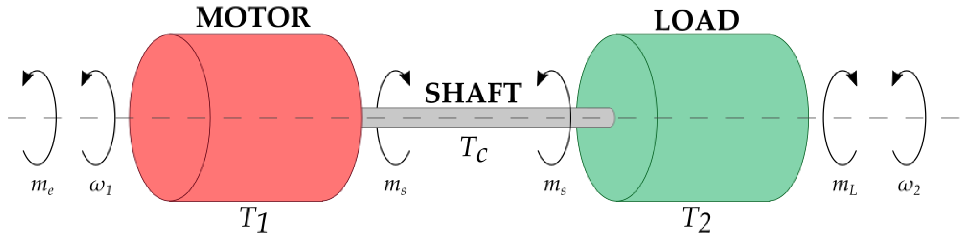
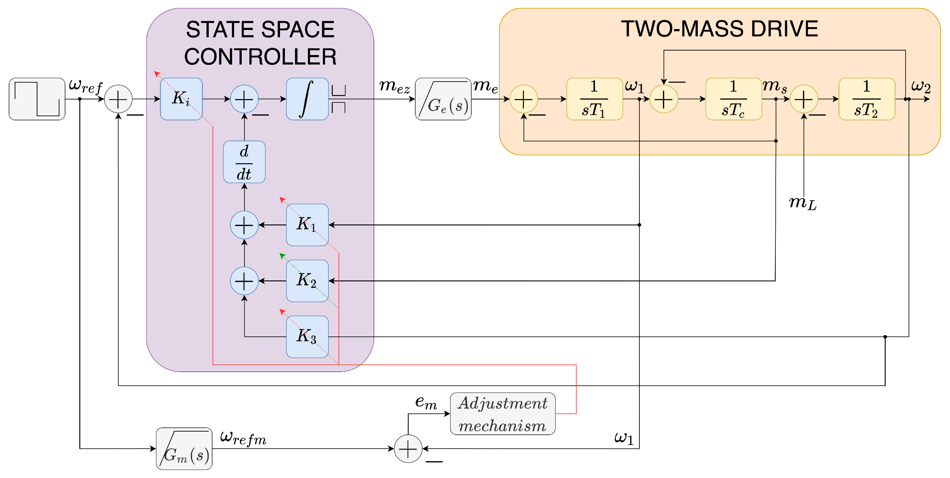
A simplified picture of the drive’s mechanical part is presented in Figure 1. The control structure analyzed in this article is based on a state controller and a two-mass drive (as presented in Figure 2).

2.1. Overall Description of the Control System

The presented model of the mechanical part of the drive can be described using the following system of differential equations [31,53,54]:

$$\begin{array}{c}\hfill \frac{\mathrm{d}{\omega }_1}{\mathrm{d}t}=\frac{m_e-m_s}{T_1}\end{array}$$

(1)

$$\begin{array}{c}\hfill \frac{\mathrm{d}{\omega }_2}{\mathrm{d}t}=\frac{m_s-m_L}{T_2}\end{array}$$

(2)

$$\begin{array}{c}\hfill \frac{\mathrm{d}{m}_s}{\mathrm{d}t}=\frac{{\omega }_1-{\omega }_2}{T_c}\end{array}$$

(3)

where ${\omega }_1$ and ${\omega }_2$ represent the rotational speed of the motor and the load (respectively), $m_e$ is the electromagnetic torque, $m_s$ is the torsional torque and $m_L$ is the load torque. $T_1$, $T_2$ and $T_c$ are the mechanical time constants of the motor, the load and the shaft connecting the two masses. In this paper, the frictional forces are not taken into account.

To represent the control structure more clearly, the torque control loop is simplified to a first-order transfer function $G_e$ with a time constant of $T_{me}$

$$G_e=\frac{1}{T_{me}s+1}$$

(4)

The whole proposed control scheme is based on a cascade structure. It consists of the inner control loop with a PI controller responsible for establishing the electromagnetic torque, and the outer loop with the proposed adaptive state feedback controller, which controls the angular velocity of the drive. It must be noted that for the purpose of this study, the drive is assumed to be fully observational (all of the state space variables are measurable). Even though the torque control loop is represented as a simple transfer function, in the practical implementation the output of the torque controller is limited. The simplification of the electromagnetic loop $G_e$ is also related to a small time constant of the current loop. It should be mentioned that with the current advances in power electronics, the delay caused by the power converter’s switches does not exceed 5 ms, which is negligible when compared to the mechanical time constant responsible for shaping the output speed. This approximation simplifies the calculation provided in the next sections.

2.2. A State Controller with Fixed Parameters Implemented for the Two-Mass System

The proposed adaptive speed controller is based on a classic state controller. The initial gain values for the adaptation process are selected as for the classic version. In the following analysis, $G_e$ is assumed to be equal 1.

In addition to the system of Equations (1)–(3), the electromagnetic torque can be described as

$$m_e=\int \left(K_i({\omega }_{ref}-{\omega }_2)-\frac{\mathrm{d}}{\mathrm{d}t}(K_1{\omega }_1+K_2{m}_s+K_3{\omega }_2)\right)\mathrm{d}t$$

(5)

which, using the Laplace operator s, can be rewritten as

$$m_e=\frac{K_i}{\mathrm{s}}({\omega }_{ref}-{\omega }_2)-(K_1{\omega }_1+K_2{m}_s+K_3{\omega }_2)$$

(6)

Parameters $K_i$, $K_1$, $K_2$ and $K_3$ are the gains of the controller (scalar values, meaning they are dimensionless). Combining Equations (1)–(3) and (6), the closed-loop transfer function can be represented as

$$\frac{{\omega }_2}{{\omega }_{ref}}=\frac{K_i}{{\mathrm{s}}^4{T}_1{T}_2{T}_c+{\mathrm{s}}^3{K}_1{T}_2{T}_c+{\mathrm{s}}^2(T_1+T_2+K_2{T}_2)+\mathrm{s}(K_1+K_3)+K_i}$$

(7)

The characteristic polynomial of the control structure has the following form:

$$H\left(\mathrm{s}\right)={\mathrm{s}}^4+{\mathrm{s}}^3\frac{K_1}{T_1}+{\mathrm{s}}^2\left(\frac{1}{T_1{T}_c}+\frac{1}{T_2{T}_c}+\frac{K_2}{T_1{T}_c}\right)+\mathrm{s}\frac{K_1+K_3}{T_1{T}_2{T}_c}+\frac{K_i}{T_1{T}_2{T}_c}$$

(8)

To obtain the values for the controller’s gains, the coefficients of the polynomial $H\left(\mathrm{s}\right)$ must be compared with the values of the coefficients in the reference polynomial $R\left(\mathrm{s}\right)$. The polynomial $R\left(\mathrm{s}\right)$ is chosen arbitrarily; however, both polynomials must be the same order. For this study, the polynomial $R\left(\mathrm{s}\right)$ is assumed as

$$R\left(\mathrm{s}\right)={({\mathrm{s}}^2+2{\zeta }_r{\omega }_0\mathrm{s}+{\omega }_o^2)}^2$$

(9)

where ${\zeta }_r$ is the desired damping coefficient, and ${\omega }_0$ is the desired resonating angular frequency. As a result of the comparison, the following equations are derived:

$$\begin{array}{cc}\hfill 4{\zeta }_r{\omega }_0& =\frac{K_1}{T_1}\hfill \end{array}$$

(10)

$$\begin{array}{cc}\hfill 2{\omega }_0^2+4{\zeta }_r^2{\omega }_0^2& =\frac{1}{T_1{T}_c}+\frac{1}{T_2{T}_c}+\frac{K_2}{T_1{T}_c}\hfill \end{array}$$

(11)

$$\begin{array}{cc}\hfill 4{\zeta }_r{\omega }_0^3& =\frac{K_1+K_3}{T_1{T}_2{T}_c}\hfill \end{array}$$

(12)

$$\begin{array}{cc}\hfill {\omega }_0^4& =\frac{K_i}{T_1{T}_2{T}_c}\hfill \end{array}$$

(13)

and finally, the expressions describing the feedback gains of the state controller are obtained:

$$\begin{array}{cc}\hfill K_1& =4{\zeta }_r{\omega }_0{T}_1\hfill \end{array}$$

(14)

$$\begin{array}{cc}\hfill K_2& =T_1{T}_c\left(2{\omega }_0^2+4{\zeta }_r^2{\omega }_0^2-\frac{1}{T_1{T}_c}-\frac{1}{T_2{T}_c}\right)\hfill \end{array}$$

(15)

$$\begin{array}{cc}\hfill K_3& =T_1{T}_2{T}_{c}4{\zeta }_r{\omega }_0^3-K_1\hfill \end{array}$$

(16)

$$\begin{array}{cc}\hfill K_i& ={\omega }_0^4{T}_1{T}_2{T}_c\hfill \end{array}$$

(17)

The expressions presented above were applied for the tuning of the controller with fixed parameters. The values were also used as the initial points for the adaptive versions of the speed controller.

2.3. Scenario 1—Partial Adaptation of the Parameters Used in the State Controller

The adaptation of weights in a simple neural model can be achieved through the use of the delta rule [55]. Here, similar calculations inspired by the fundamentals from the theory of artificial intelligence are proposed. In the state controller, the feedback coefficients are used to recalculate the signal values. Then the signals are combined into one element (a sum of values, similar to a neuron with a linear activation function). In order to reduce the state error, an additional integral element is often implemented (main path with error). In consequence, a form of integral control with state feedback is obtained.

In these considerations, for the updates of the speed controller gains, a simplification is assumed–-direct multiplication (without integration) is considered. Additionally, the basic form of the full state feedback controller is analyzed. According to the conditions mentioned above, additional issues related to the limitation of signals are omitted. Then, the output of the state controller (the reference electromagnetic torque value), can be rewritten as follows:

$$m_{ez}=-K_{i}e-K_1{\omega }_1-K_2{m}_s-K_3{\omega }_2$$

(18)

where:

$$e={\omega }_{ref}-{\omega }_2$$

(19)

The main goal of coefficient optimization is to reduce the error defined as

$$e_m={\omega }_{refm}-{\omega }_1$$

(20)

where ${\omega }_{refm}$ is obtained by passing the reference signal ${\omega }_{ref}$ through a model of the desired dynamics. In this paper, the model takes the following form:

$$G_m\left(s\right)=\frac{{\omega }_0^2}{s^2+2{\zeta }_r{\omega }_{0}s+{\omega }_o^2}$$

(21)

The parameters of the state controller are updated using the following formulas:

$$\begin{array}{cc}\hfill K_i(k+1)& =K_i\left(k\right)+\mathsf{\Delta }{K}_i\left(k\right)\hfill \end{array}$$

(22)

$$\begin{array}{cc}\hfill K_1(k+1)& =K_1\left(k\right)+\mathsf{\Delta }{K}_1\left(k\right)\hfill \end{array}$$

(23)

$$\begin{array}{cc}\hfill K_3(k+1)& =K_3\left(k\right)+\mathsf{\Delta }{K}_3\left(k\right)\hfill \end{array}$$

(24)

where k is the number of the current iteration.

The novelty of the presented research lies within the adaptation of the variable $K_2$. The proposed adaptation algorithm for $K_2$ will be described in the subsequent section. Before that, the updates of the $K_i$, $K_1$, and $K_3$ are analyzed. First, Equations (22)–(24) are redefined:

$$\begin{array}{cc}\hfill K_i(k+1)& =K_i\left(k\right)-\alpha g_i\left(k\right)\hfill \end{array}$$

(25)

$$\begin{array}{cc}\hfill K_1(k+1)& =K_1\left(k\right)-\alpha g_1\left(k\right)\hfill \end{array}$$

(26)

$$\begin{array}{cc}\hfill K_3(k+1)& =K_3\left(k\right)-\alpha g_3\left(k\right)\hfill \end{array}$$

(27)

where $\alpha$ is the adaptation coefficient, and $g_i$, $g_1$ and $g_3$ are the partial derivatives of the error function with respect to their corresponding variables:

$$\begin{array}{cc}\hfill g_i\left(k\right)& =\frac{\partial E\left(k\right)}{\partial K_i}\hfill \end{array}$$

(28)

$$\begin{array}{cc}\hfill g_1\left(k\right)& =\frac{\partial E\left(k\right)}{\partial K_1}\hfill \end{array}$$

(29)

$$\begin{array}{cc}\hfill g_3\left(k\right)& =\frac{\partial E\left(k\right)}{\partial K_3}\hfill \end{array}$$

(30)

The mentioned error function E can be taken from the neural network theory. It can be defined as

$$E=\frac{1}{2}{\left(d\left(k\right)-y\left(k\right)\right)}^2=\frac{1}{2}{\left(e_m\left(k\right)\right)}^2$$

(31)

where d is the desired value from the model, and y is the output value. For this application, the output of the neural model y can be defined using (18). According to the issues considered above, the adjustments of the gains in the analyzed controller are described with the following equations [56]:

$$\begin{array}{cc}\hfill \mathsf{\Delta }{K}_i(k+1)& =-\alpha e_m\left(k\right)e\left(k\right)\hfill \end{array}$$

(32)

$$\begin{array}{cc}\hfill \mathsf{\Delta }{K}_1(k+1)& =-\alpha e_m\left(k\right){\omega }_1\left(k\right)\hfill \end{array}$$

(33)

$$\begin{array}{cc}\hfill \mathsf{\Delta }{K}_3(k+1)& =-\alpha e_m\left(k\right){\omega }_2\left(k\right)\hfill \end{array}$$

(34)

The definition of the correct value is hard to describe using mathematical formulas. Thus, in this work, the selected metaheuristic algorithms were applied for this purpose.

The stability of the presented structure can be analyzed in two main ways. The experimental and the theoretical approaches can be adopted. To check the stability of the given system, the trial and error method for different values of the initial weights and the learning coefficients can be applied. On the other hand, there are theoretical methods for ensuring the stability of a given system. One of the most commonly used methods is the Lyapunov’s stability theorem. It is applied in a wide range of plants with adaptive controllers. However, this work is focused on the implementation and tests of a modified adaptive state controller.

2.4. Scenario 2—A Novel Approach to the Adaptive State Space Controller—Indirect Adaptation of $K_2$

The first version of the adaptive state controller uses recalculation of the parameters based on the speed error. The gain of the path with the $m_s$ signal is constant. This assumption is related to problems with the accessibility of the reference signal for the torsional torque. Otherwise, the method (from the previous section) of adaptation should be extended also for the $K_2$ parameter. However, the speed and the torque have different dynamics and shapes; they eliminate the adaptation of this coefficient similar to the others. Thus, an additional modification is proposed. Using Equations (14)–(17) the formula for $K_2$ can be rewritten as

$$K_2=2T_1{T}_c{\omega }_0^2(1+2{\zeta }_r^2)-\frac{T_1}{T_2}-1$$

(35)

The following can also be observed

$$\begin{array}{cc}\hfill T_1& =\frac{K_1}{4{\zeta }_r{\omega }_0}\hfill \end{array}$$

(36)

$$\begin{array}{cc}\hfill T_2& =\frac{K_i}{T_1{T}_c{\omega }_0^4}=\frac{4K_i{\zeta }_r}{K_1{T}_c{\omega }_0^3}\hfill \end{array}$$

(37)

By inserting (36) and (37) into (35)

$$K_2=\frac{K_1{T}_c{\omega }_0}{2{\zeta }_r}-\frac{K_1^2{T}_c{\omega }_0^2}{16{\zeta }_r^2{K}_i}+K_1{T}_c{\zeta }_r{\omega }_0-1$$

(38)

After recalculations, the new formula for $K_2$ is achieved:

$$K_2=\frac{K_1{T}_c{\omega }_0(8K_i{\zeta }_r-K_1{\omega }_0)}{16{\zeta }_r^2{K}_i}+K_1{T}_c{\zeta }_r{\omega }_0-1$$

(39)

With this description, the parameter $K_2$ now becomes indirectly subjected to adaptation. It is dependent on other gains of the controller ($K_i$ and $K_1$), which are already changing their value, causing $K_2$ to also change its value alongside them. What is worth noting is that now, that value is independent from the time constant of the load machine $T_2$, which is the most changing part for this expression.

3. Nature Inspired Optimization Algorithm—The Symbiotic Organism Search

The symbiotic organism search is a nature-inspired algorithm that simulates the behavior of organisms spotted in their natural habitats [57]. None of the organisms live alone. The relationships between them can be described as symbiosis, which stands for “living together”, where two or more species bring benefits to one or more parties involved. Depending on the result of the symbiosis, different relationships can be formed: commensalism, mutualism, and parasitism. Mutualism is the most common form of symbiosis between different species where two organisms benefit from the relationship. Commensalism describes the two organisms living together, where only one benefits but the other one is not harmed. The third relationship, parasitism, benefits only the parasite, while the other organism, called the host, is harmed. The SOS describes only the three aforementioned relationships from all six possible relationships.

The SOS uses the population of organisms to solve the numerical optimization task over the course of many iterations. The generated population is used to model the three symbiotic behaviors. A member of the population or ecosystem is randomly generated with constraints to the limits of the optimization task:

$$x_i=UB+rand(0,1)·(UB-LB)$$

(40)

where x is the newly generated solution, i is the number of the specimen, and LB and UB are the lower and the upper bounds of the optimization problem, respectively. Then, the fitness function for the whole ecosystem is evaluated, and the best candidate should be found—the one with the lowest value of the fitness function for the minimization problems. In this paper, the following fitness function is used:

$$F_{cost}=\sum _{k=1}^N\frac{|{\omega }_1\left(k\right)-{\omega }_2\left(k\right)|}{N}$$

(41)

where N is the number of samples of the simulation.

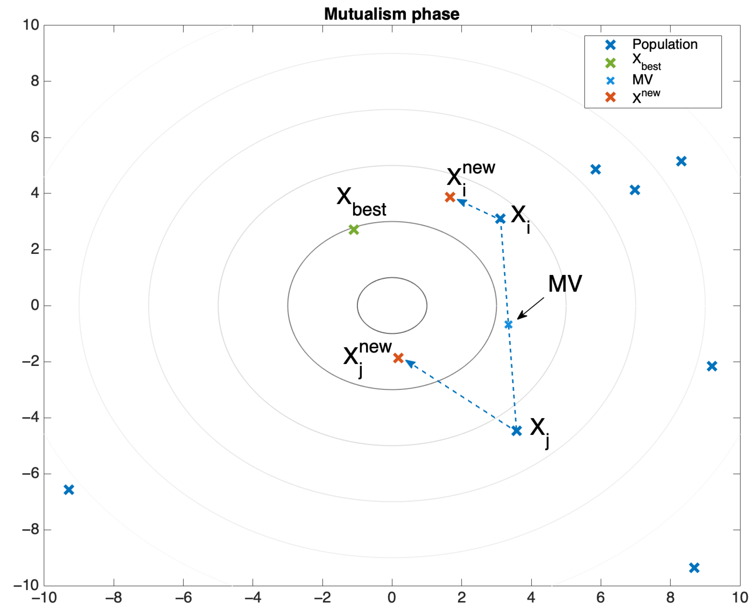
After finding the best organism, the mutualism phase takes place. As in all forms of symbiosis, two organisms are needed, so apart from the currently selected individual $x_i$, another one ($x_j$) is randomly selected from the population. Both organisms are coupled for a mutualistic relationship, the goal of which is to increase the survival rate of both. To calculate the new solutions, mutual vector (MV), as well as beneficial factors (BF) should be calculated first [58].

$$MV=\frac{x_i+x_j}{2}$$

(42)

MV represents the relationship between both organisms, while BF models the level of benefit from i or j organism. BF is randomly selected as 1 or 2. New values of $x_i$ and $x_j$ are then created using the following formula [50]:

$$x_i^{new}=x_i+rand(0,1)·(x_{best}-MV·B{F}_1)$$

(43)

$$x_j^{new}=x_i+rand(0,1)·(x_{best}-MV·B{F}_2)$$

(44)

where $x_{best}$ is the fittest individual.

$x_{best}$ is incorporated into Equations (43) and (44) as the population tries to evolve according to Darwin’s law—“survival of the fittest”. Later, the fitness function of the evolved organism is evaluated. If the new values are better, $x^{new}$ takes the place of x; in the other case, x is saved in the ecosystem. The effect of the mutualism phase and the effect of $MV$ is presented in Figure 3 below.

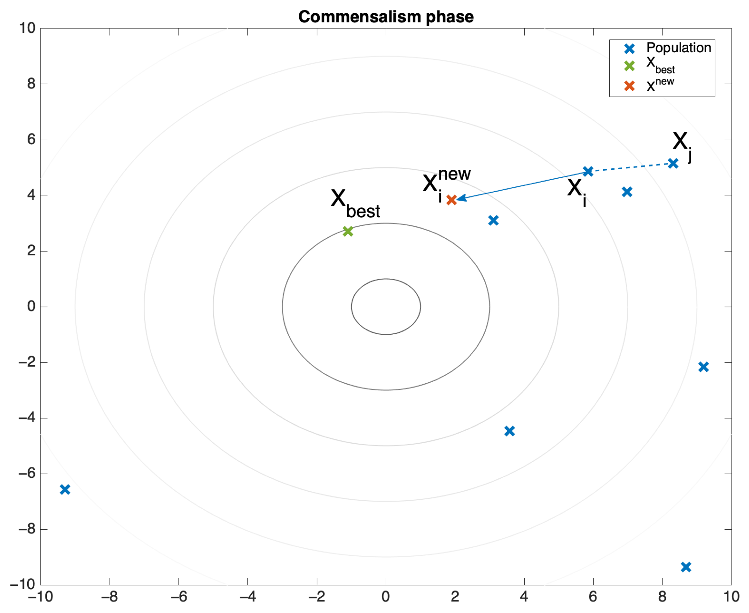
The commensalism phase comes later, where only one organism benefits from the relationship. It can be modeled in the same way without the usage of the MV and BF. The new value of the organism is generated based on the best individual and the randomly selected organism (45) [59].

$$x_i^{new}=x_i+rand(-1,1)·(x_{best}-x_j)$$

(45)

The effect of the commensalism phase is depicted in Figure 4.

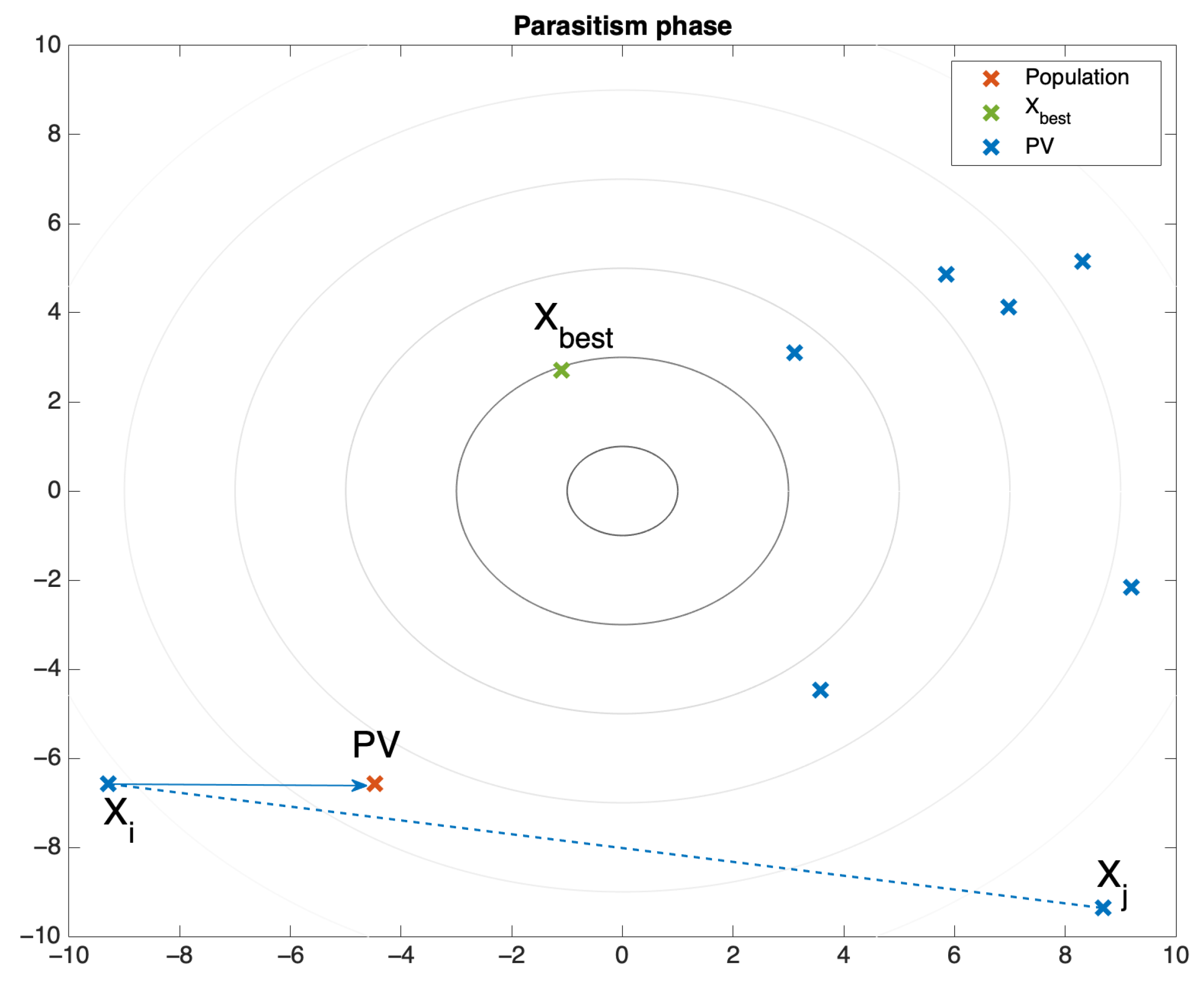
The last part of the algorithm consists of the parasitism phase. The parasitism phase utilizes the so-called parasite vector (PV) [60]. It is created by duplicating and modifying random dimensions from a selected organism $x_i$. Then, another organism $x_j$ is randomly selected that can be treated as a host to a parasite $x_i$. The goal of the parasite is to replace the host in the ecosystem. The fitness function of both organisms is evaluated, and the fittest one stays in the population. If the PV has a better value of the fitness function, it replaces the host position in the ecosystem. Otherwise, if the host is immune to the parasite, it is saved in the population and the PV is erased. There are many different ways to implement the parasitism phase. In some cases, creating the PV just means creating a new organism [50,61]. In other implementations, some dimensions are changed, and this is dependent on the version of the algorithm [57,59]. This application changes only one dimension of the selected organism. 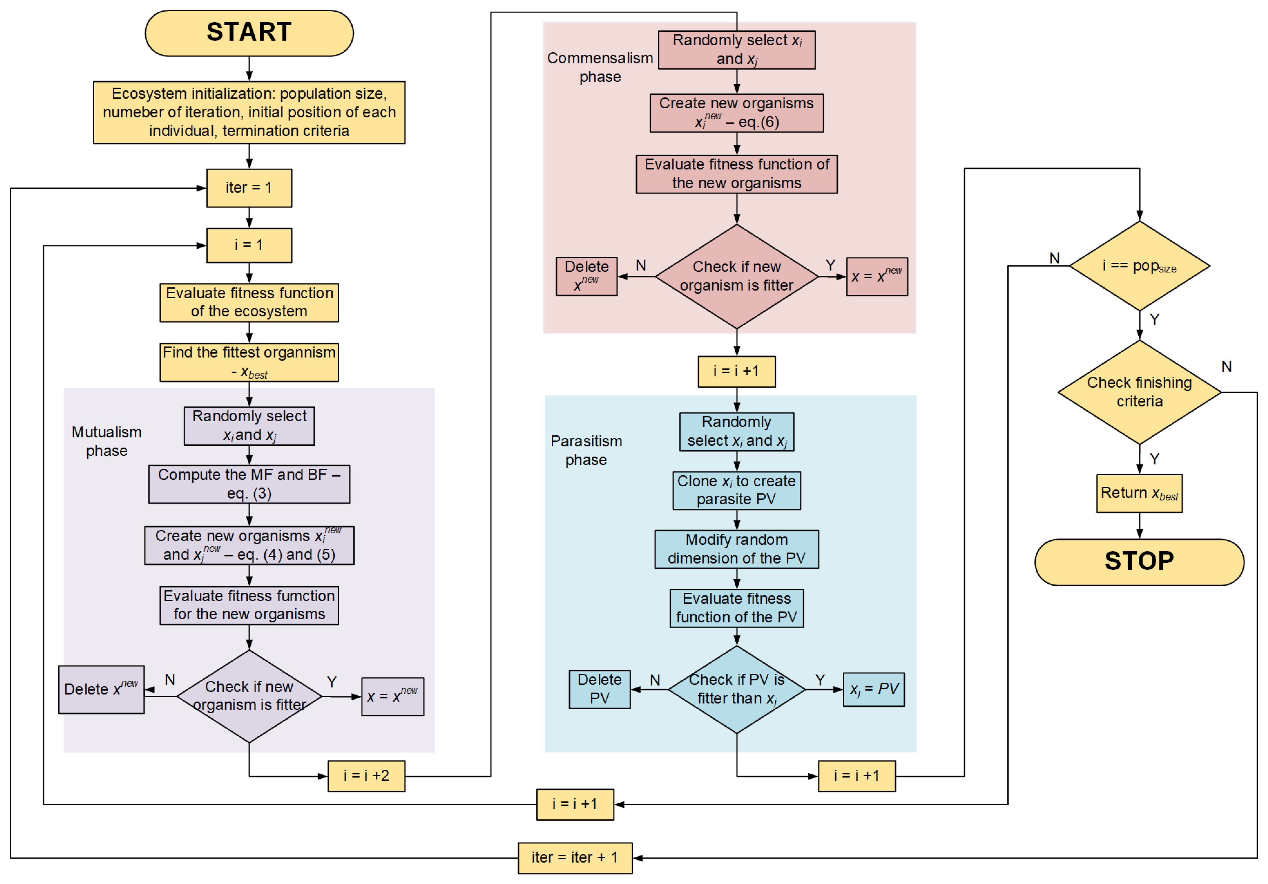The visualization of the last phase is shown in Figure 5. The basic parameters of the SOS are presented in

Table 1. Parameters of the symbiotic organism search algorithm.

Parameter	Value
Population size	20
Main loop iteration count	20
$[LB,UB]$	$[-0.5,0]$
Max. time for a main loop	120 min

below. The whole algorithm can be summarized in the block diagram depicted in Figure 6.

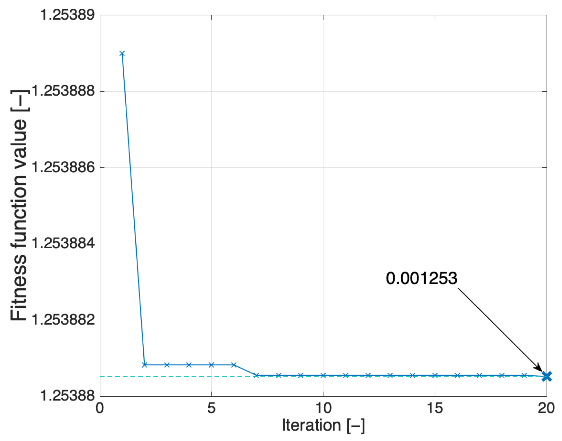
Changes in the fitness function are presented in Figure 7 below. The minimum value achieved by the algorithm was equal to $F_{cost}=1.253\times {10}^{-3}$, it was also marked with the light blue transient. As presented, even the value achieved in the first iteration was close to the final result, which shows that this task was relatively simple for a metaheuristic algorithm to calculate.

4. Nature Inspired Optimization Algorithm—The Flower Pollination Algorithm

Currently, a significant increase in applications of metaheuristic optimization algorithms may be observed, especially for solving non-linear, complex functions. As it was presented in the introduction of the paper, a few parameters of the controller have to be determined in order to ensure the expected dynamics of the plant. The presented method of pole placement may only be used if all parameters of the controlled plant are properly identified [12]. That method is not appropriate for closed-loop control when any elements of artificial intelligence are employed. The stability issues may be observed in such cases when the controller is tuned with the standard method. This is caused by the fact that during the synthesis, such elements are not taken into account in the mathematical model of the control structure [62]. However, the issue may be eliminated by the approach of the direct tuning of closed-loop systems. The initial controller coefficients may be tuned during the operation of the plant. However, the more efficient and safer solution is to perform the tuning during simulations. There are different algorithms that may be employed for such a task [63]. In this paper, the nature-inspired algorithms were examined. For comparison purposes, the tuning was also conducted with the flower pollination algorithm.

The flower pollination algorithm is a metaheuristic algorithm that mimics the natural process of pollen transfer. The algorithm was presented by Xin-She Yang in 2012 [64]. The algorithm is a universal tool for optimization in different areas of science, economics and also social behavior studies [65,66,67,68]. It belongs to swarm-based metaheuristic algorithms. This means that in every iteration, the initial population is improved because only the strongest specimens are able to survive. The strength of every specimen equals the value of the fitness function. Because the tuning process is a minimization task, the smaller the obtained value of the cost function, the better the solution. In the considered application, the same cost function that was employed with the SOS algorithm was proposed. The difference between the angular velocity of the electrical motor and the load machine is calculated for every sample. Then the mean of the absolute values is calculated.

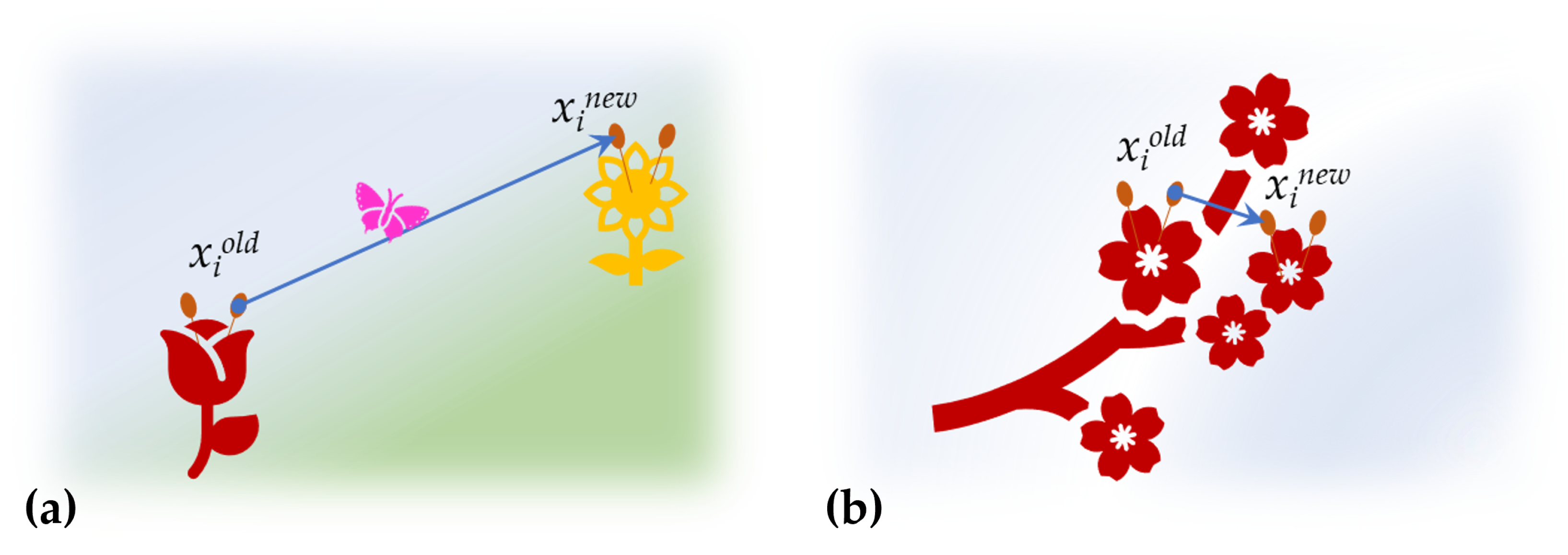
The flower pollination algorithm is based on the observations of pollen transfer. Two processes of this phenomenon may be differentiated in nature. The first one is called cross-pollination, and it requires the specimens of two different plants to take part. Because of the fact that the pollen has to be moved over longer distances in cross-pollination, pollinators (insects) are required to move pollen between distant flowers (Figure 8a). The movement of the insects is considered a global, random process. This leads to the suggested mathematical model of such movement, called Lévy flight (46). The random movement is obtained by the $\mathsf{\Gamma }\left(\lambda \right)$ parameter [69].

$$L=\frac{\lambda \mathsf{\Gamma }\left(\lambda \right)sin\left(\frac{\pi \lambda }{2}\right)}{\pi s^{1+\lambda }}$$

(46)

where $\mathsf{\Gamma }\left(\lambda \right)$ is the standard gamma function for the index $\lambda$, s is a random step size from the Lévy distribution.

The second mechanism of pollen transfer is independent from external creatures and may be driven only by wind. It employs flowers of the same plant, and is called self-pollination (Figure 8b). This process allows the plant to survive; however, the features of the new specimen are very similar to its predecessors. Because of that, it is considered local and depends only on specimens from the current population.

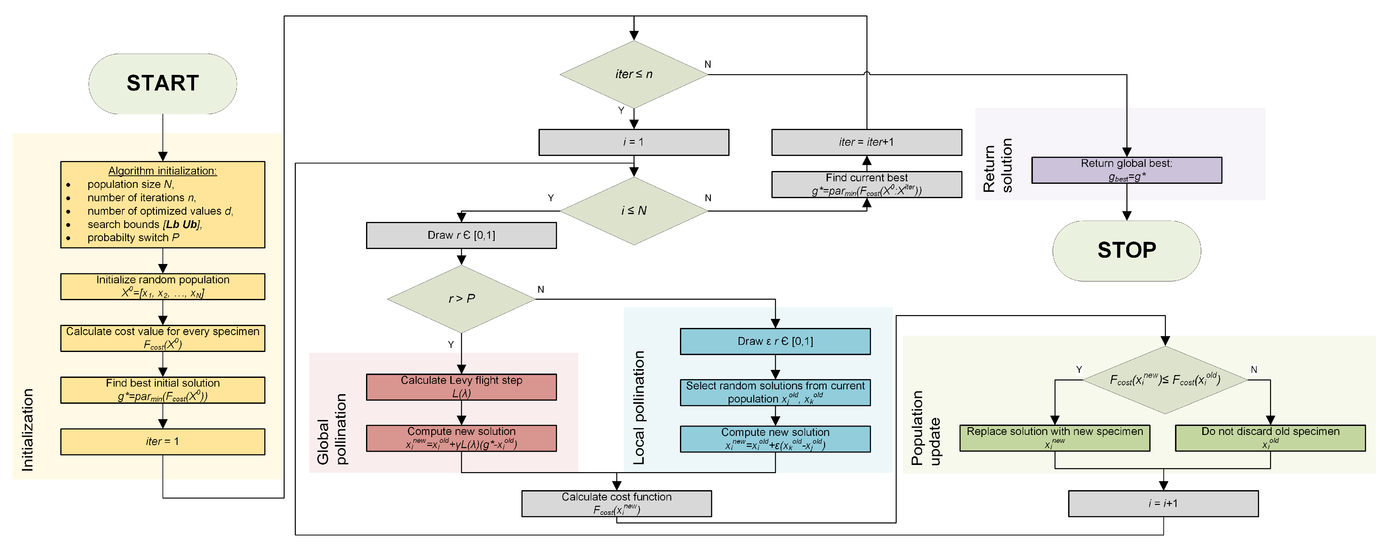
Global and local optimization is required to obtain satisfactory results. Global optimization ensures that the calculations do not stop at the local extremum and the global minimum is obtained, while local optimization is required to obtain even better approximation of the fittest solution. These two mechanisms are switched randomly in every iteration. The drawn value r is compared to the probability switch parameter P. Depending on the value of r, the current iteration may be calculated either as global optimization (Equation (47)) or local optimization (Equation (48)). After the new solution is calculated, the cost function value is checked. If the improvement is noted, the ı-th specimen in the population $x_i^{old}$ is replaced with a new solution $x_i^{new}$. After all the iterations are computed, the global best result is returned. The flow of data during the optimization with the FPA is shown in Figure 9.

$$\begin{array}{c}\hfill x_i^{new}=x_i^{old}+\gamma L\left(\lambda \right)(g^{*}-x_i^{old}),\end{array}$$

(47)

$$\begin{array}{c}\hfill x_i^{new}=x_i^{old}+ϵ(x_j^{old}-x_k^{old}),\end{array}$$

(48)

where $x_i^{new}$ is the new solution, $x_i^{old}$ is the value of the i-th specimen in the current population, $\gamma$ is the step size for the global pollination, $L\left(\lambda \right)$ is the calculated Lévy flight step, $g^{*}$ is the current best solution, $ϵ$ is a random step size for the local pollination from Gaussian distribution, and $x_j^{old},x_k^{old}$ are values of two specimens chosen from the current population.

For research purposes, in order to receive comparable data, the population size was set to 20 specimens, and only 20 iterations were considered. The optimized variable was the $\alpha$ coefficient, which is responsible for the adaptation speed. The bounds of the search range were defined basing on the knowledge about $\alpha$ presented in [70]. All parameters are gathered in

Table 2. Parameters of the flower pollination algorithm.

Parameter	Value
Population size	20
Main loop iteration count	20
Probability switch P	0.8
$[L_b,U_b]$	$[-0.5,0]$

.

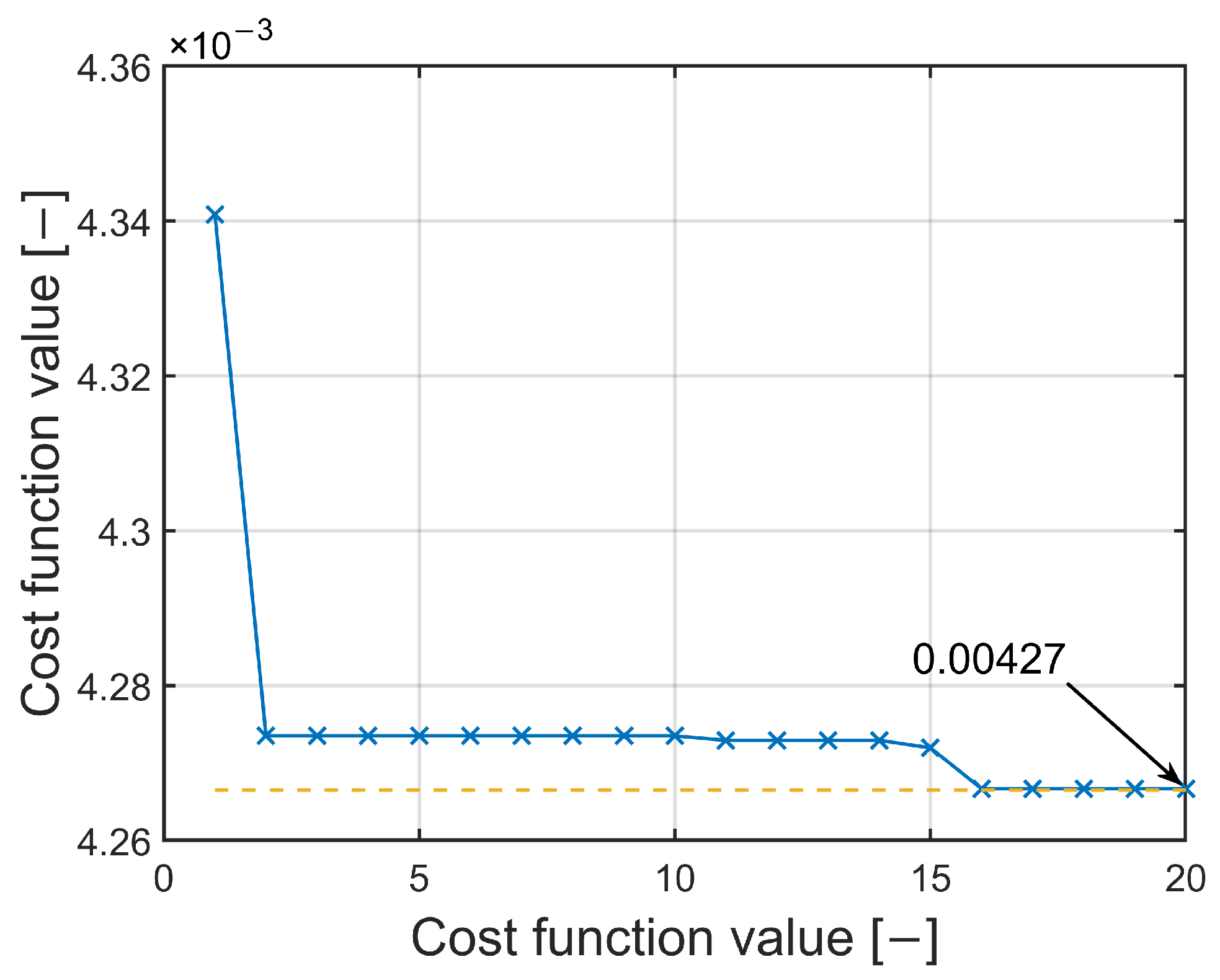
Even a small number of computed main loop iterations leads to improvement. The values of the fitness function in consecutive iterations are shown in Figure 10. In the given example, the obtained minimum value of the fitness function is equal to $F_{cost}$$=4.27\times {10}^{-3}$. As it was already noted in the SOS description, the very first iteration quickly improves the solution close to the global best.

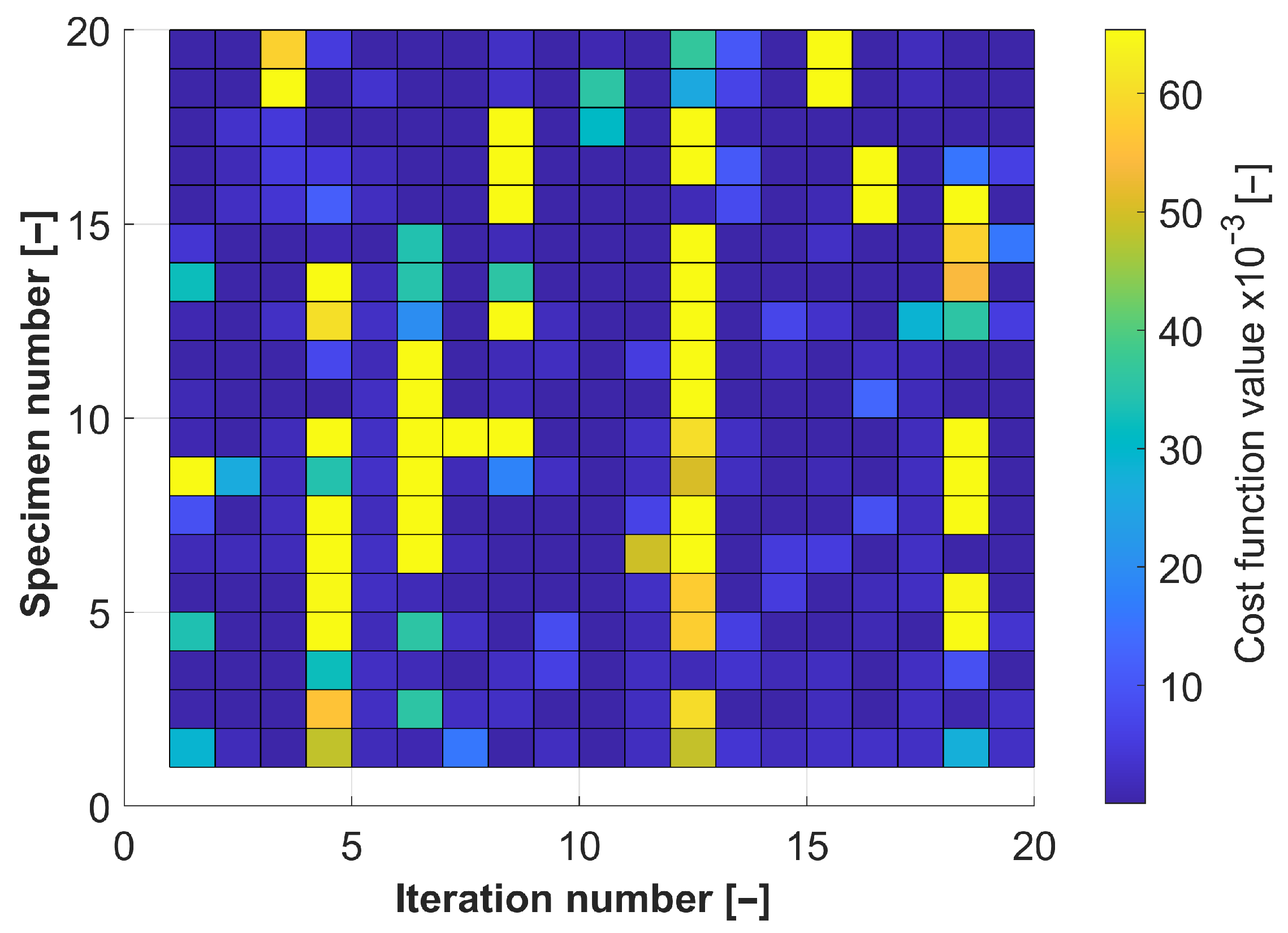
Because the process is based on the development of the populations-the improvement of every specimen in following iterations can be observed (Figure 11). This inheritance-based approach improves the optimization efficiency.

Both presented algorithms use a pseudo-random number generator, which is a common practice in the meta-heuristic approach. The goal of the optimization process is to find a point close to the global minimum of the fitness function. Finding a point that is a global minimum is not always guaranteed when nature-inspired algorithms are used. The optimization process gives only the starting point to the gradient-based algorithm presented in the previous section. Then, the goal of the learning process of the controller is to obtain the global minimum point.

5. Simulation Tests

Simulation tests were carried out using the MATLAB/Simulink environment. The control structure was implemented in Simulink, and the data were fed through the MATLAB workspace. During the simulation time of $t_{sim}=20$ s, the drive performs reversions with the amplitude of ${\omega }_{ref}=0.25$ p.u. The load torque is applied in $t_{ml}=13.2$ s of simulation with a nominal value. All the state space variables were saved during the simulations.

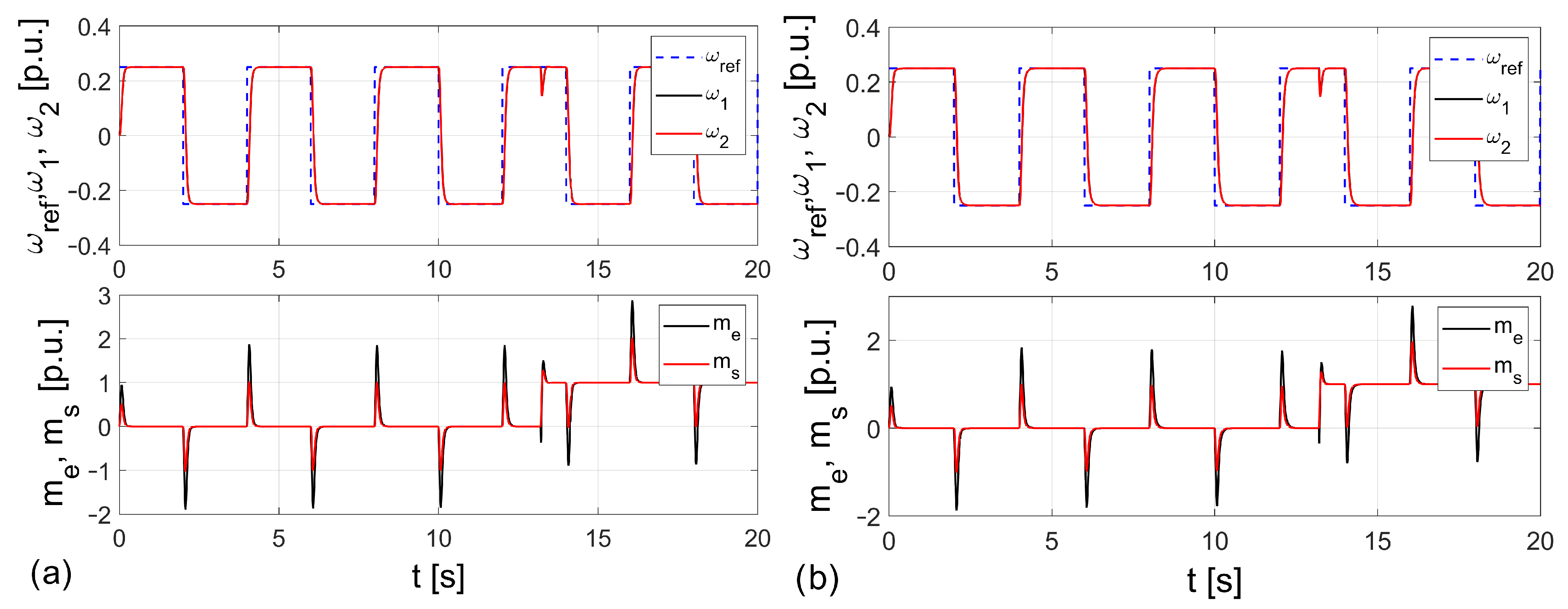
The main point of this paper is to show that the adaptive state space controller can be implemented in many ways. One of them is to set the initial values of the adaptive gains as calculated in Equations (14)–(17), and optimize the value of the adaptation parameter $\alpha$. Transients for the nominal case for the SOS and the FPA optimization are shown in Figure 12. There is no overshoot or oscillations present in the speed transients. The drive precisely follows the reference speed. A high level of control accuracy is observed. The reaction of the state variables after the load switching is dynamic. Even though both figures look similar, the optimization parameter $\alpha$ slightly differs between the algorithms. The SOS optimization yields ${\alpha }_{SOS}=0.0341$, and the FPA yields ${\alpha }_{FPA}=0.0312$. 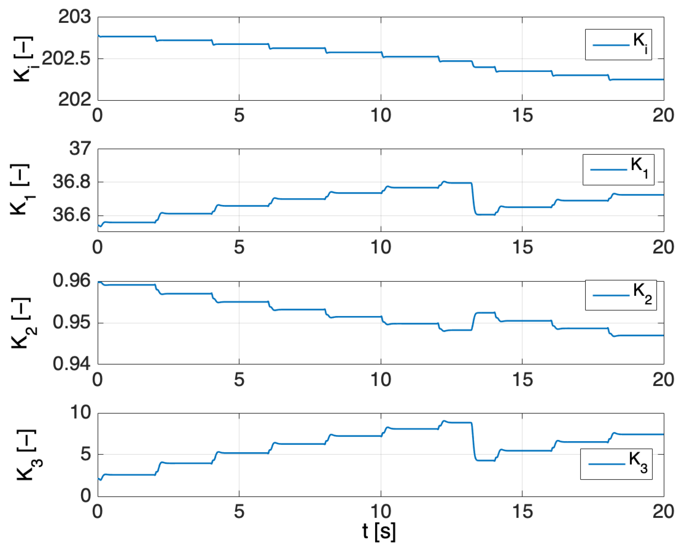Correct adaptation can be noticed in the changes of the gains (Figure 13). Values of the adaptive parameters are changed after every reversion of the drive. It can also be seen that the load torque also has an impact on the values of the weights.

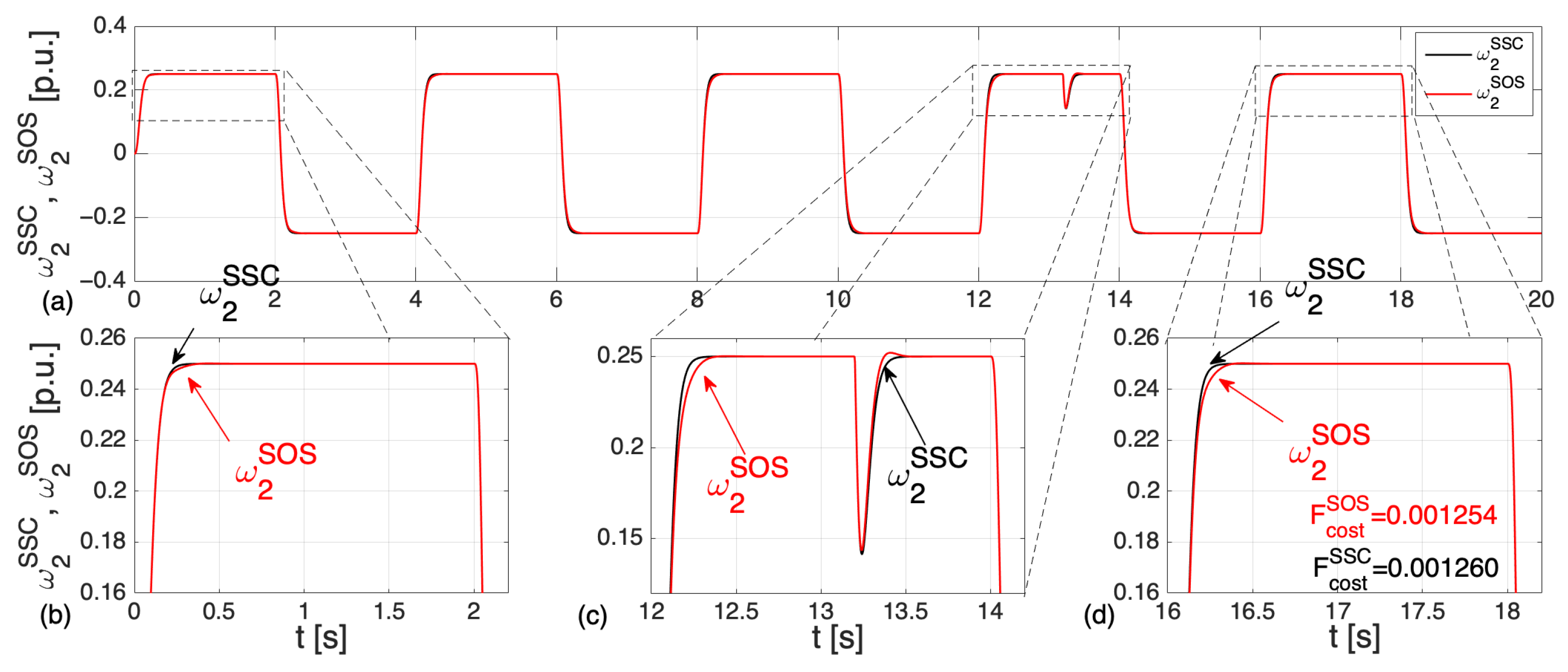
To show the improvement over the classic state space controller, a comparison of the optimized adaptive structure (by the SOS) and the state space controller is also presented. The difference between drive performance with the SSC and the adaptive optimized controller (with only the value of the adaptive coefficient optimized) is shown in Figure 14a, and the zooms in Figure 14b–d. A minimal overshoot is visible after the load torque is applied. The speeds of both structures are similar during the course of the simulation, but the fitness function $F_{cost}$ is slightly smaller in the adaptive scenario, which proves that the presented structure has higher dynamics.

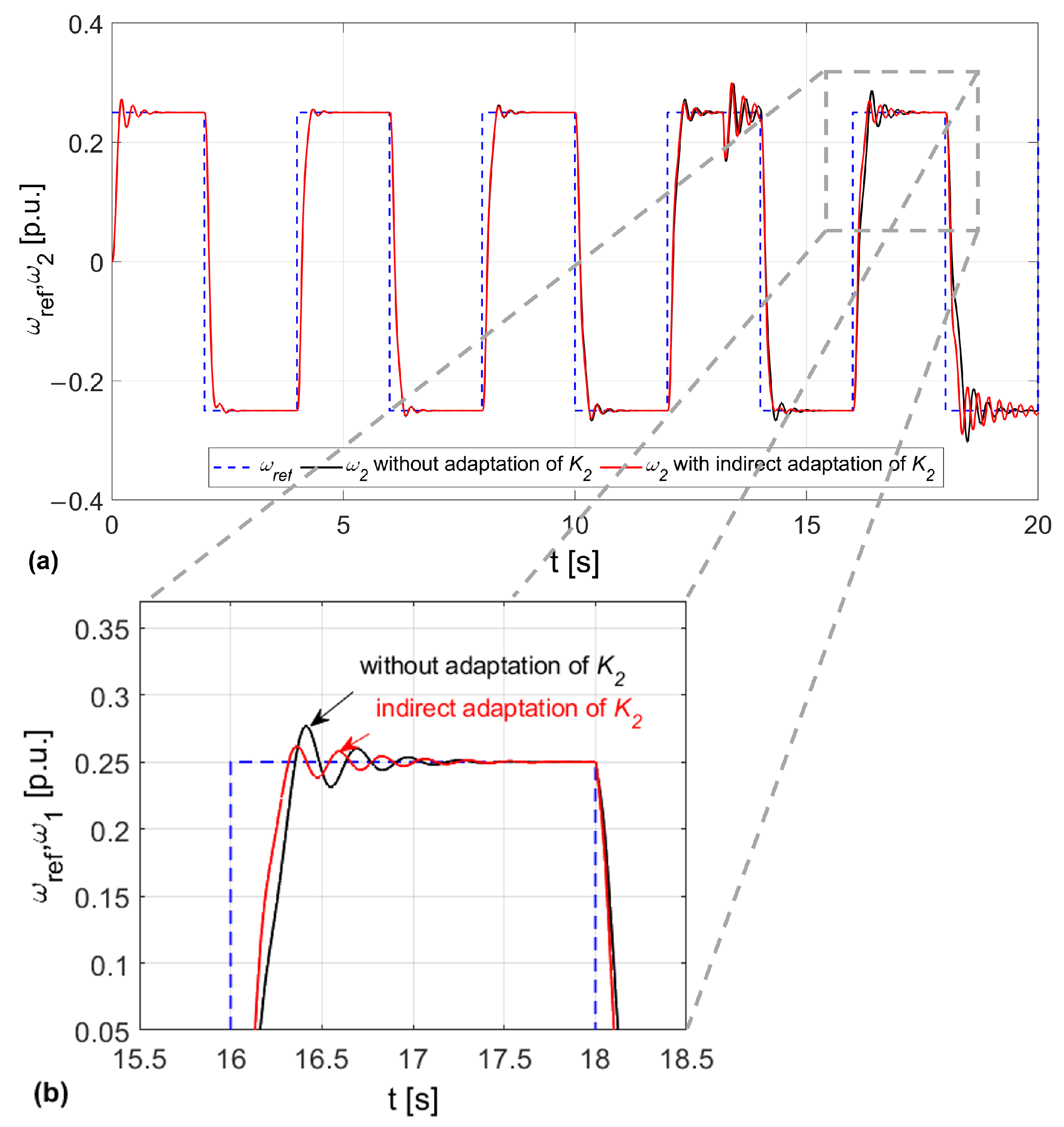
The novelty of the presented structures lies in the indirect adaptation of the gains of the controller; it shows significant improvement for the dynamics of the drive. Comparison of classic adaptive state controller and the novel structure is shown in Figure 15. As it can be seen in the figures, a significant increase in adaptation of speed is observed when all coefficients are adaptable. Not only is the response quicker, but also the overshoot is clearly smaller (Figure 15b).

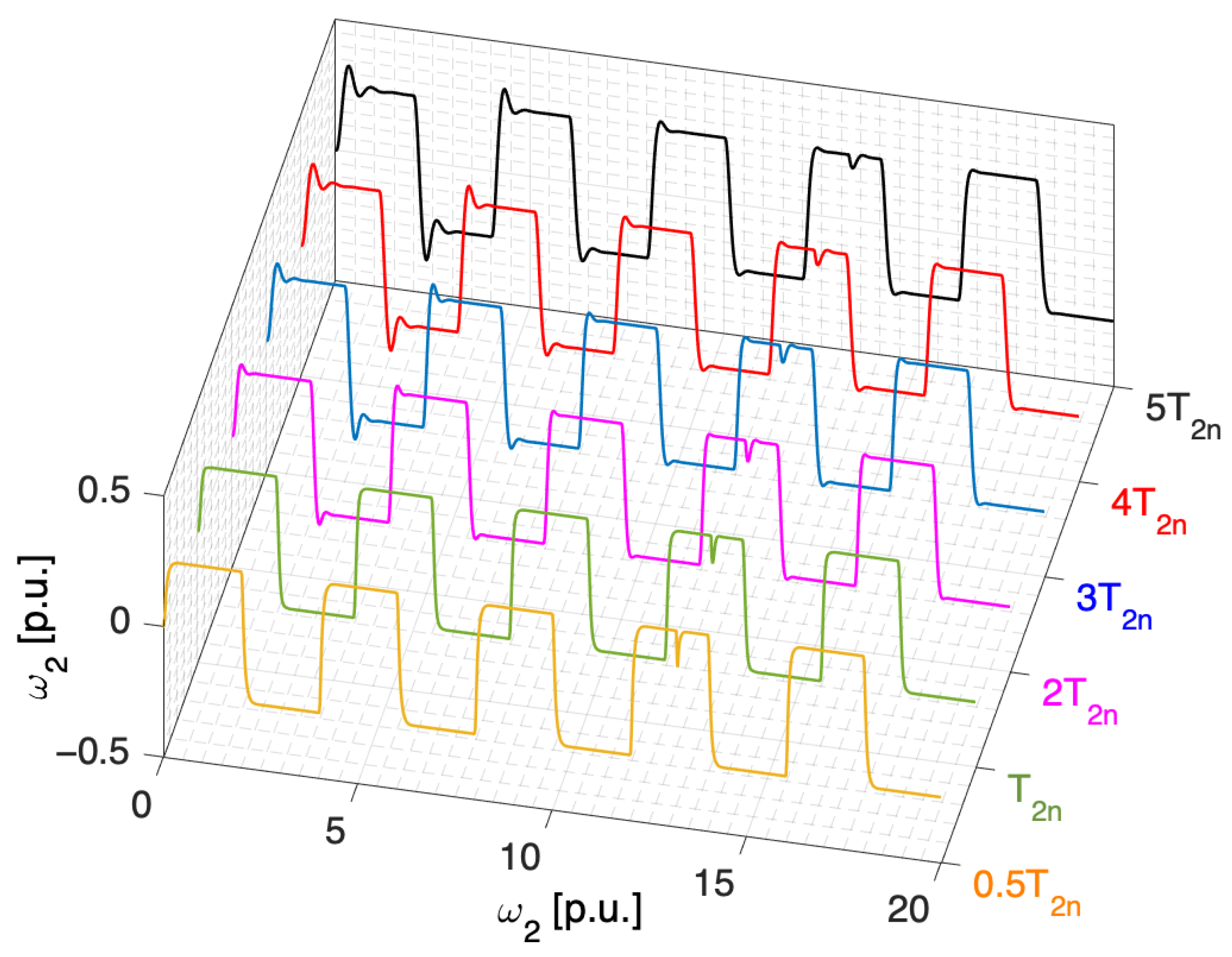
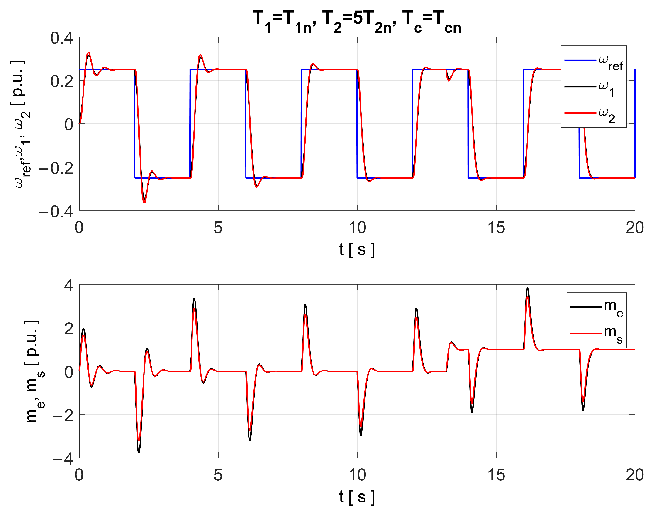
Robustness against changes of the load time constant was also tested (Figure 16).

As the load time constant increases, the overshoot is higher in the startup process of the drive. Even though the time constant rises, overshoot is diminished due to the changes in the gains of the controller. The maximum overshoot for the drive with the load time constant increased five times is about 36%. Lowering the load machine time constant increases the reaction to the load torque; other than that, the drive works in the same manner.

Similar tests were conducted for the FPA algorithm (optimization of all parameters of the controller). Figure 17 shows transients of the speeds and torques obtained for the changed load time constant. Only the worst case—$T_2=5T_{2n}$—is presented, as the previously shown results (Figure 12) confirm that both algorithms yield similar solutions.

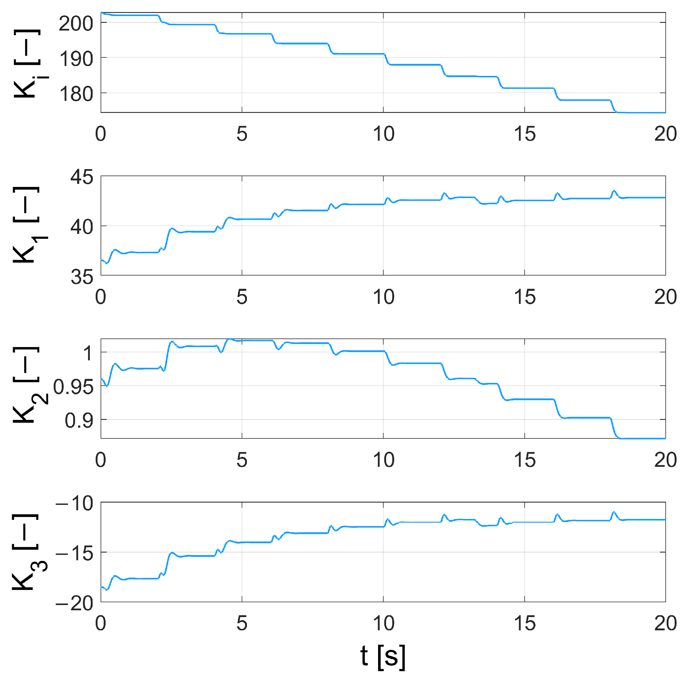
The adaptation process is undoubtedly visible—the initial $20\%$ overshoot is well damped after four reversions. The change (adaptation) of the state controller gains is presented in Figure 18. It is clear that the initial values of gains are not optimal for the plant (when the load time constant is increased). In comparison to the gains presented in Figure 13, the range of change is greater. During the first reversions, rapid change of the coefficients is observed after about 10 s. $K_1$ and $K_3$ settle at a stable level. It is worth indicating that the indirect adaptation of $K_2$ is also visible. At the beginning, the value increases and then starts to decrease after every reversion.

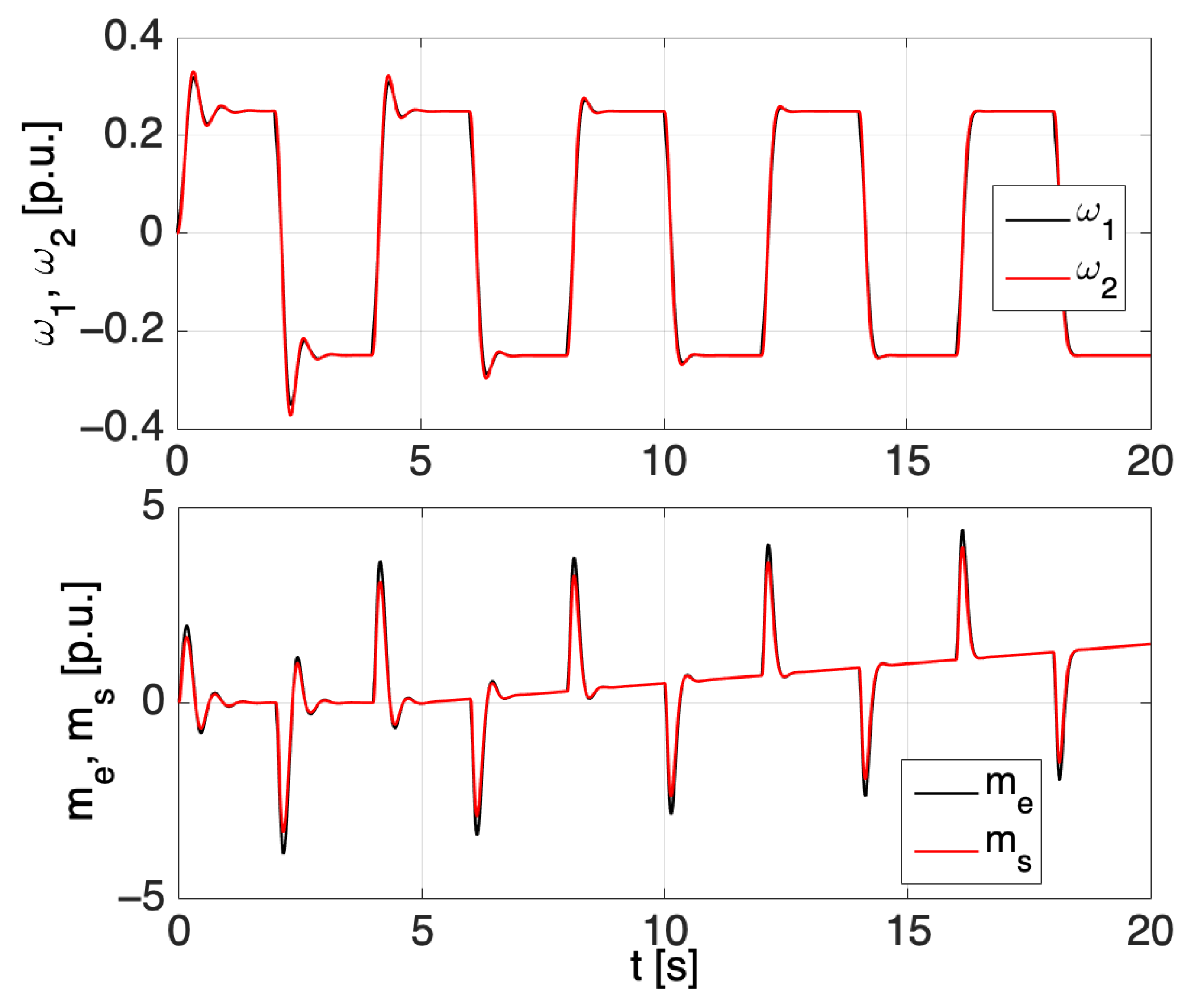
The load torque (disturbance) in the previous tests was applied as a sudden appearance of the nominal value to test the robustness of the system. Such an example is rare in real applications. Thus, other tests were performed. The gradual changes (slope) of the load were also analyzed. After the initial phase (adaptation of the weights), the control system works stably. The load does not influence the precise tracking of the reference trajectory. However, the current values become higher in each reverse of the drive (Figure 19).

Another way of implementing the adaptive state space controller is to optimize the initial values of the controller ($K_i$, $K_1$, $K_2$, $K_3$) as well as the learning coefficient. In this approach, all the values were optimized by an metaheuristic algorithm, which means that such parameters as ${\zeta }_r$ and ${\omega }_0$ cannot be determined. Thus, it means that the dynamics of the structure are entirely selected by the algorithm and the fitness function.

The fully optimized structure by the SOS algorithm is presented in Figure 20. There is a minimal overshoot as the speed recovers from the application of the load torque. The dynamics of the whole structure are similar to the one calculated using Equations (14)–(17), which proves that the SOS (or any other metaheuristic algorithm) can find the solution near the optimal point (depending on the fitness function and the difficulty of the problem). The torque is generated in a fast manner, and it is not saturated by the limits of the speed controller.

The influence of the load time constant $T_2$ was also checked and is presented in Figure 21. The overshoot of the load speed, in the startup operation of the drive, increases alongside the increase in $T_2$, though it is always damped as the adaptation progresses. Although the time constant of the load machine is high, the drive can follow the reference speed precisely or with a minimal overshoot.

6. The Experimental Verification

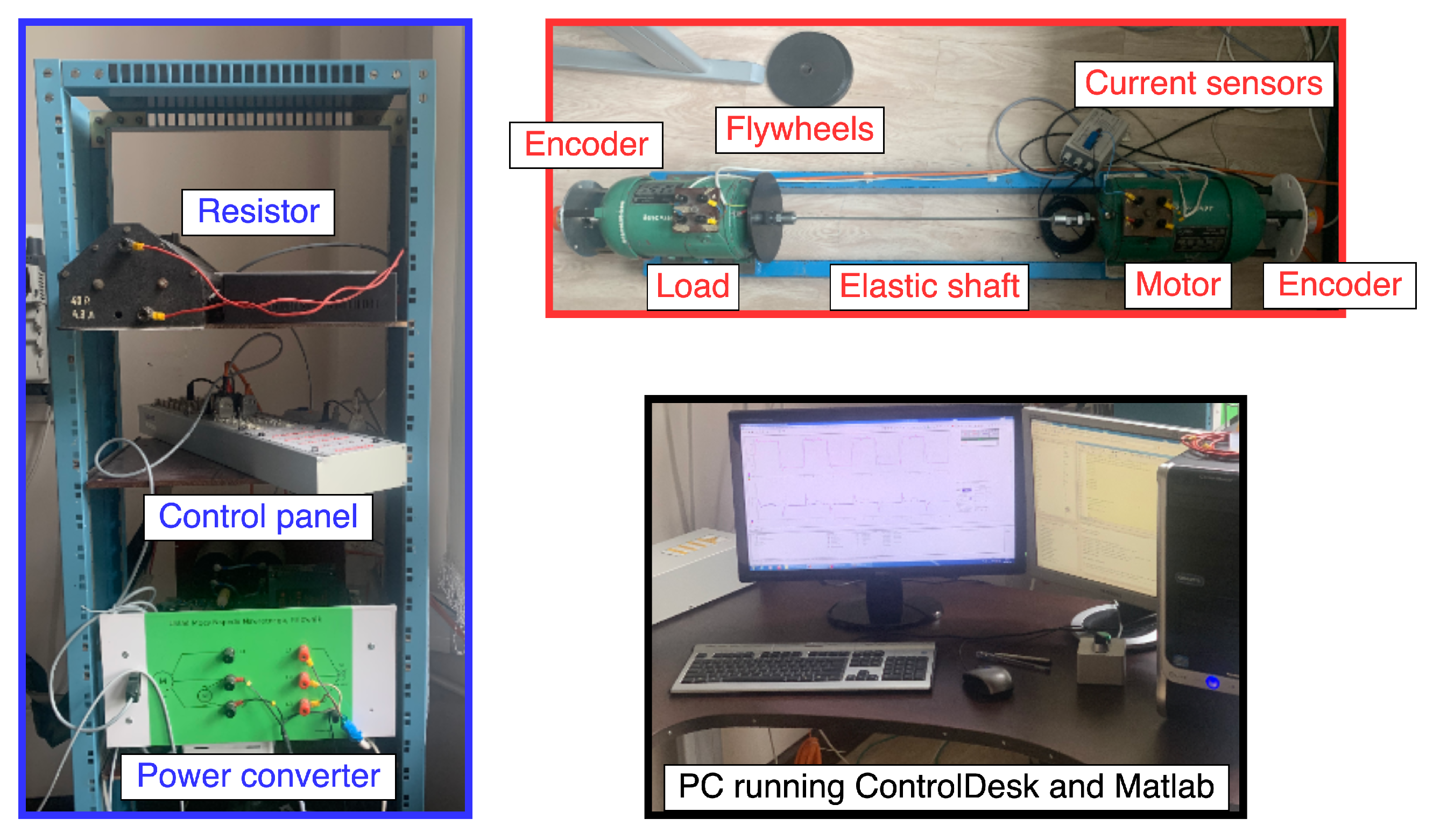
In order to confirm the satisfactory dynamics obtained with simulations, the results were also verified with laboratory equipment. In this part of the paper, the hardware implementation and the initial results are described. The laboratory stand consists of two electrical motors (with the nominal power of 0.5 kW) connected with a flexible shaft. While the first motor is the controlled plant, the second one acts as the load. Time constants of the system may be changed by adding flywheels and replacing the shaft. The control structure is implemented on dSPACE 1103 card. The current feedback is realized with LEM sensors, and the speed feedbacks are achieved with encoders attached to each of the motors. 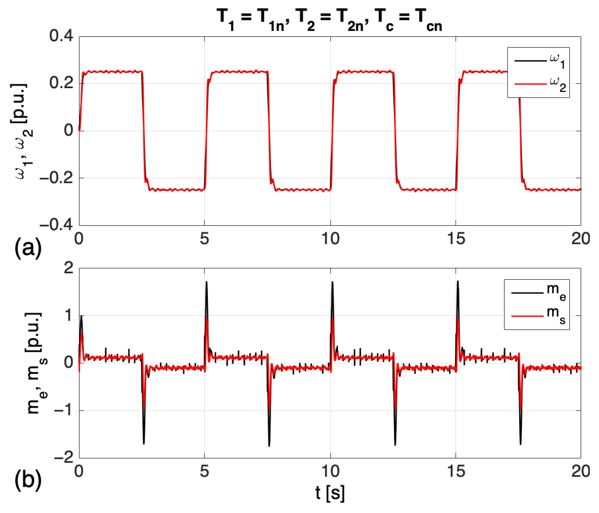The laboratory stand is shown in Figure 22. The first tests were conducted for the nominal parameters of the drive and the standard state space controller in order to check if the plant was correctly identified for simulations. The results proved that the response of the plant is similar to the modeled one.

In the next step, the suggested novel adaptive controller with indirect adaptation of $K_2$ was tested. Figure 23 shows the speed of the motor and the load with adaptive controller (scenario 2 in Section 2.4). These tests were initially performed for the nominal parameters of the drive and the state space controller with optimized value of $\alpha$. Stable work of the system and precise tracking of the reference signal as well as the high dynamics of the generated torque are observed.

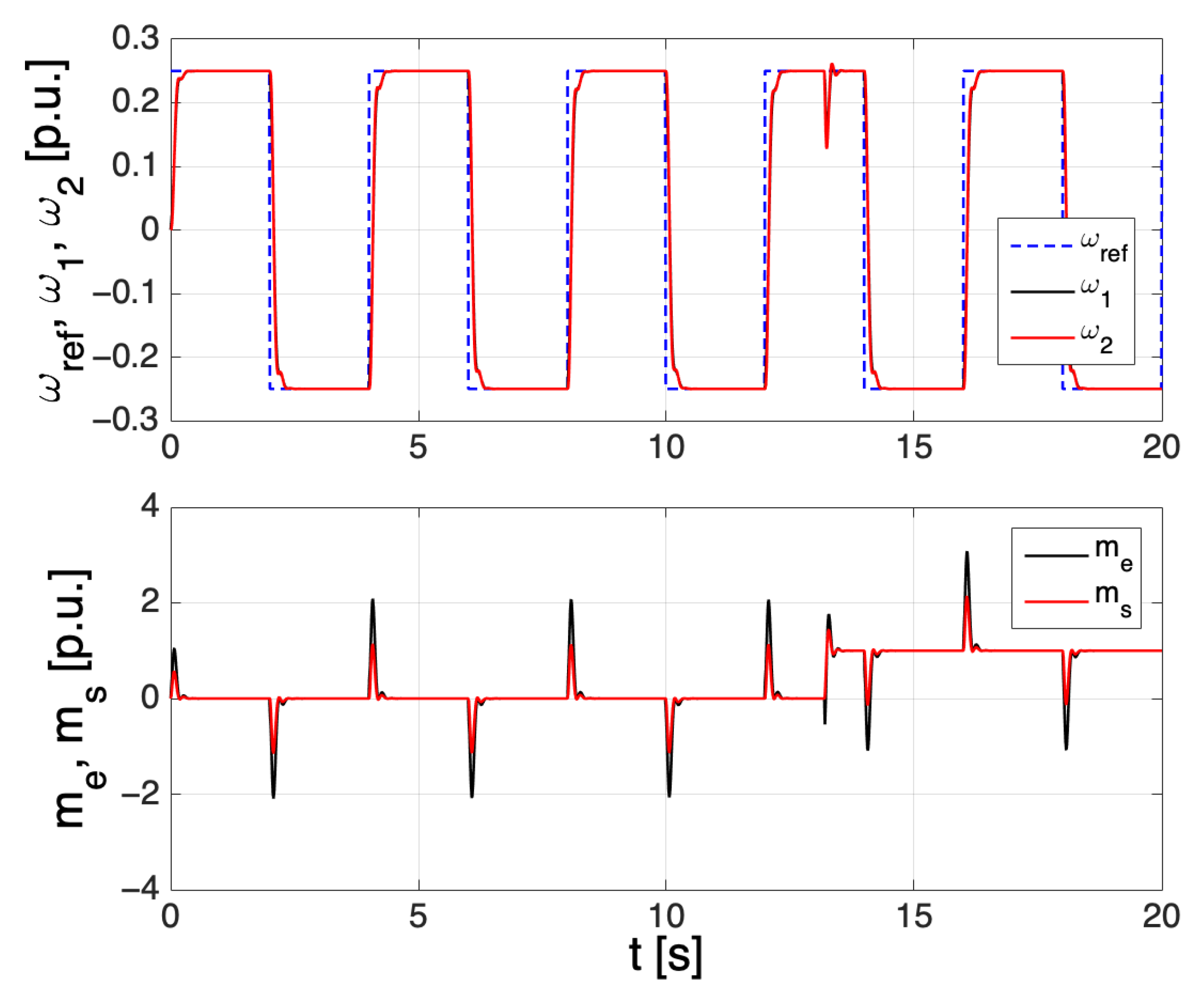
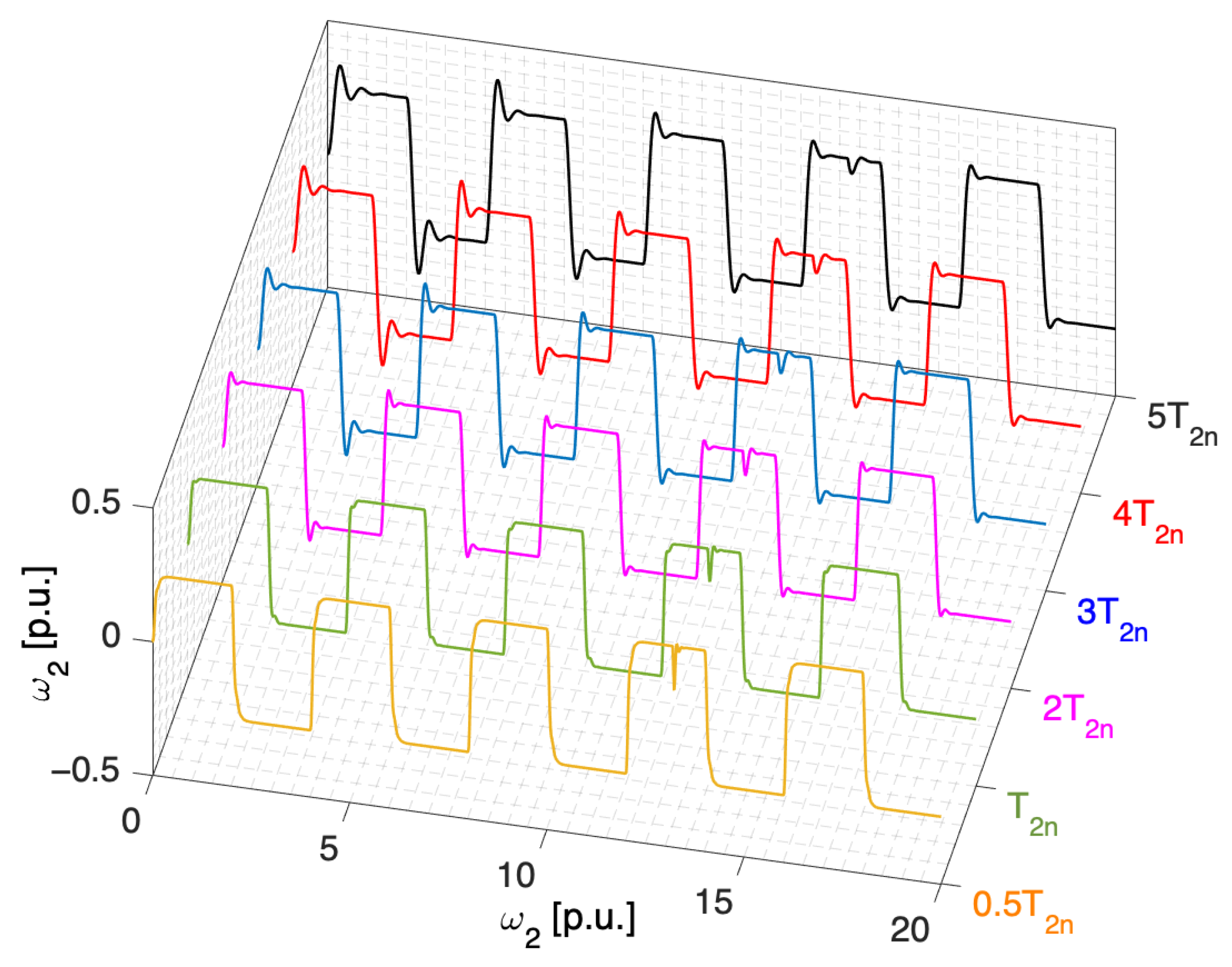
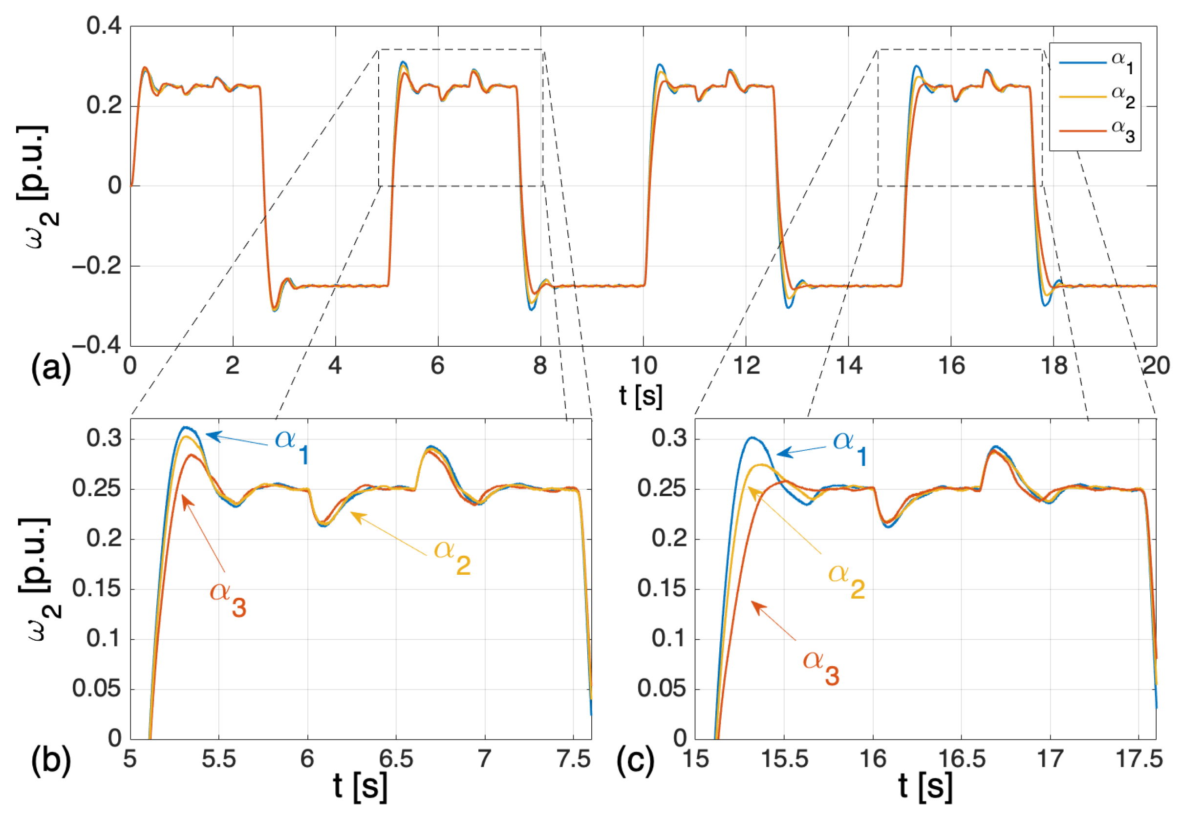
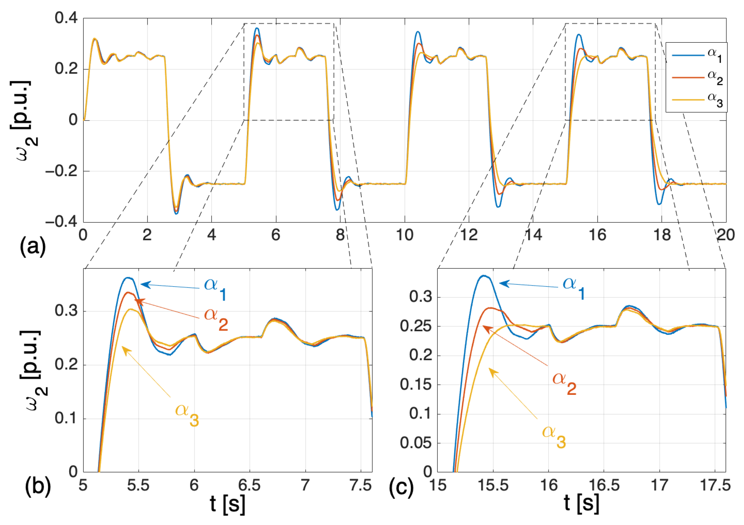
Next tests were conducted for the scenario where the identification of the plant was performed inaccurately or the load of the drive was changed. This was obtained by the change of $T_2$ variable through the attachment of additional flywheels to the second motor shaft. The results with a higher time constant of the load machine-$3T_{2n}$ are presented in the figure below. Different values of the adaptation parameter $\alpha$ were applied in increasing order (${\alpha }_1<{\alpha }_2<{\alpha }_3$). Experimental results prove the results obtained in the simulation part. As the adaptation coefficient increases, the overshoot is reduced for the startup part of the experiment. Overshoot is damped during the process of adaptation in every reversion. It is also observed when an additional flywheel is added to the shaft (for the sum of $5T_{2n}$).

The second part of the test shows work of the control structure after changes of the mechanical time constant of the load ($T_2$). Results with higher time constant of the load machine ($3T_{2n}$) are presented in Figure 24 and Figure 25 for $5T_{2n}$. Different values of the adaptation parameter $\alpha$ are applied—in increasing order (${\alpha }_1<{\alpha }_2<{\alpha }_3$). The experimental results prove the results obtained in the simulation part. The main trend is similar: as the adaptation coefficient increases, the overshoots are more quickly reduced. The adaptation process leads to damping of the oscillations and correct operation after parametric disturbances.

Even the significant increase of $T_2$ can be handled by the proposed adaptive controller. The transients presented below show that the unwanted oscillations are not present, even for the situation where $T_2=5T_{2n}$.

7. Concluding Remarks

The paper deals with different approaches to a state controller applied for a two-mass system. The initial structure has a typical form, which uses signals from the mechanical part of the drive. Then, additional adaptation for the parameters of the controller is implemented. Two solutions of the adaptive speed control are considered (novel indirect method of adaptation of one of the coefficient was also considered). Selected optimization techniques are used to optimize the value of the learning rate of the controller as well as the initial values. The use of the metaheuristic algorithms provides an easy and efficient tool for the design stage. The indirect method of adaptation (for the $K_2$ parameter) improves the dynamics of the drive and its work under changes of the plant parameters. Another law of adaptation implemented for this coefficient is needed due to this parameter’s dependency on the fast changing torsional torque (the remaining gains are based on the angular velocities). The simulation results show high efficiency in damping the oscillations caused by the torsional torque in the electrical drive with an elastic joint. This confirms the possibility of the correct application of the presented structure. The initial experimental results were obtained using the dSPACE card to confirm the correct operation of the proposed control structure. Comparison of the efficiency achieved with the presented adaptive structure and basic controllers such as a PI controller or a state space controller indicates a significant improvement. Not only are the oscillations damped, but also the overshoots are minimized, resulting in a reduction in the cost function value of about 40%. Further research will be focused on the implementation of the algorithms on a low-cost device and the stability analysis.