Analyzing and Forecasting Multi-Commodity Prices Using Variants of Mode Decomposition-Based Extreme Learning Machine Hybridization Approach

Abstract

Because of the non-linearity inherent in energy commodity prices, traditional mono-scale smoothing methodologies cannot accommodate their unique properties. From this viewpoint, we propose an extended mode decomposition method useful for the time-frequency analysis, which can adapt to various non-stationarity signals relevant for enhancing forecasting performance in the era of big data. To this extent, we employ variants of mode decomposition-based extreme learning machines namely: (i) Complete Ensemble Empirical Mode Decomposition with Adaptive Noise-based ELM Model (CEEMDAN-ELM), (ii) Ensemble Empirical Mode Decomposition-based ELM Model (EEMD-ELM) and (iii) Empirical Mode Decomposition Based ELM Model (EMD-ELM), which cut-across soft computing and artificial intelligence to analyze multi-commodity time series data by decomposing them into seven independent intrinsic modes and one residual with varying frequencies that depict some interesting characterization of price volatility. Our findings show that in terms of the model-specific forecast accuracy measures different dynamics in the two scenarios namely the (non) COVID periods. However, the introduction of a benchmark, namely the autoregressive integrated moving average model (ARIMA) reveals a slight change in the earlier dynamics, where ARIMA outperform our proposed models in the Japan gas and the US gas markets. To check the superiority of our models, we apply the model-confidence set (MCS) and the Kolmogorov-Smirnov Predictive Ability test (KSPA) with more preference for the former in a multi-commodity framework, which reveals that in the pre-COVID era, CEEMDAN-ELM shows persistence and superiority in accurately forecasting Crude oil, Japan gas, and US gas. Nonetheless, this paradigm changed during the COVID-era, where CEEMDAN-ELM favored Japan gas, US gas, and coal market with different rankings via the Model confidence set evaluation methods. Overall, our numerical experiment indicates that all decomposition-based extreme learning machines are superior to the benchmark model.

1. Introduction

The efficient functioning of markets for natural gas, coal, and crude oil among others is quite relevant for the rational allocation of scarce resources and for the effective and timely attainment of environmental targets such as climate change mitigation, and of the goal toward achieving a net-zero carbon economy. The current soaring prices of energy can be related to different factors. For instance, this includes the rebound of demand after the lock-downs—specifically, an era where a vaccine is found, and a lot of people have been vaccinated. In addition to the aforementioned, there was a drop in renewable electricity penetration from a lack of wind in Europe during larger parts of the year 2021 (https://www.wsj.com/articles/soaring-energy-prices-only-the-beginning-climate-change-net-zero-renewable-wind-electricity-11641417084 (accessed on 24 February 2022). However, energy market prices keep on fluctuating from time to time, which makes the market unpredictable most of the time and hence, requires various sophisticated prediction models for both short-term forecast and long-term forecast.

One characterization of the energy market is its fluctuation. This remains a fact in that while prices are on the excessively high side, the market continues to be hugely unpredictable, and it becomes increasingly a difficult task for anyone to provide a view on the trajectory of the prices in the long term. Nevertheless, these predictions are quite relevant for various market players including consumers and prosumers. In this paper, we focus on the log-price changes of commodity prices under consideration. For example, most historical data do reflect the complexity of volatility characterizations of energy market prices namely: (i) non-linearity, (ii) uncertainty, and (iii) dynamics, thus making the forecasting of these prices a daunting task. This normally influences and causes significantly high uncertainties that may finally cause significant turmoil, which affects the returns of related investors. In effect, it disrupts and negatively influences the steady development of our social economy, which describes the current state of the world because of COVID-19 and the tension in Ukraine. Specifically, this tension has sent global crude oil prices to record highs, with the Brent price surging above US$105/bbl on 24 February 2022 for the first time since summer 2014, and the US West Texas Intermediate (WTI) exceeding US$100/bbl (https://www.enerdata.net/publications/daily-energy-news/us-plans-oil-release-after-ukraine-related-surge-global-crude-oil-prices (accessed on 26 February 2022). As mentioned by [1], the price volatility of energy assets such as natural gas, crude oil, and coal among others do influence electricity prices, which altogether directly have significant economic impacts on different sectors of the economy. This, therefore, provides a natural platform to account for accurate price changes and volatility forecasts. In other words, accurate energy price volatility and changes in price predictions are very valuable for the reliable and stable operational security of energy systems. To this extent, it is worthwhile analyzing all these four commodities because of the significant role they play in the energy system starting from their industrial consumption as well as individual consumers.

On the other hand, in this dispensation of big data, correctly harnessing data, and thus, providing accurate forecasts can aid better and fact-based decision-making. This dispensation has seen very fast and unpredictable changes, where several people are connected to each other through mobile devices and the Internet of things (IoT)/and Internet of Everything (IoE), and as such most of the product that surrounds us is becoming more complex day by day. This cannot be achieved by traditional models and hence the need for cutting-edge research methods such as artificial intelligence and soft computing either stand-alone or in combination with traditional models can provide an improved modeling framework relevant for decision making. In this light, we employ a combination of models namely the Complementary Ensemble Empirical Mode Decomposition with Adaptive Noise-based ELM Model (CEEMDAN-ELM), the Ensemble Empirical Mode Decomposition Based ELM Model (EEMD-ELM), and the Empirical Mode Decomposition Based ELM Model (EMD-ELM) to investigate multi-commodity prices in terms of their forecasting performances. Notably, the original empirical mode decomposition model (EMD) pioneered by [2] provides a self-adaptive decomposition approach, which enhances the forecast accuracy of non-linear and non-stationary time series data. As indicated by these authors, their main conceptual innovations lie in the introduction of the intrinsic mode functions which depend on the local properties of the signal and contribute positively to the instantaneous frequencies, thereby eliminating other representations for non-linearity and non-stationary via spurious harmonics. Meanwhile, this approach has seen several extensions in the works of [3,4,5] among many others. Some recent papers that use combined forecast include ([6] Section 2.6); who highlight the fact that given several forecasts of similar events, then, the forecast combination is set forth to estimate the combined weights of each forecast such that the accuracy of the combination of forecasts outperforms the forecast accuracy of the individual forecasts. From this viewpoint, this paper utilizes the univariate forecast as the benchmark and the combined forecast to examine the energy commodity prices.

On the other hand, as mentioned by ([6] Section 3.4), when there is an extensive expert dispersion in the panel of forecasts being combined, it is likely that some individual ones might appear to be outliers. In this case, a single expert forecast might suffice instead of relying on the whole sample of forecasts. In effect, Ref. [7] argued that combining a small crowd might be powerful in practice, creating some form of diversity. In addition, Ref. [6] (Section 3.4.6) pointed out that collaborative forecasting in the energy sector, which reflects the combination of geographically distributed time-series data, is capable of delivering significant improvements in the forecasting accuracy of each renewable energy power plant. This shares similitude with our modeling approach, which utilizes different modeling frameworks to examine energy commodities and exploit their forecasting performances, thereby delivering significant enhancement in forecast accuracy. Also, the quest to accurately forecast energy commodities seems to always pose a challenge for several reasons. For example, Ref. [8] suggested that crude oil price evolution is inherently not predictable. Nonetheless, this perception is changing, given various promising forecast models, which our approach seeks to contribute to and thus provide new insights. Motivated by the aforementioned issues, a hybrid model that combines various decomposition models with extreme learning machines is proposed for forecasting energy commodities. Apart from the combined models, we select a univariate forecasting model as our benchmark, specifically, in a similar framework of [9], the autoregressive integrated moving average model (ARIMA) is utilized to forecast the price return series of energy commodities.

The main contribution and motivation for this study is to propose variants of ensemble empirical mode decomposition-based extreme learning machine approach for energy commodity price forecasting and compare its predictive ability among the competing variant forecasting techniques. From a broad perspective and to the best of our knowledge, there is no paper, that utilizes our proposed hybrid model in the forecasting of multi-commodity energy prices, and therefore, this paper provides a benchmark, which could be applied in other related markets. In view of the competitive advantages and benefits of econometric models in combination with soft-computing methods in depicting and capturing the non-linearity, and dynamic features, our proposed method is suitable for multi-commodity price forecasting. For robustness check, we consider two scenarios namely (i) before the COVID-19 period and (ii) during the COVID-19 outbreak, to provide a clear-cut and meaningful insight into the adaptability of the modeling framework in (non)-stressful times. Furthermore, the introduction of a univariate benchmark model showcases the fact that the decomposition-based extreme machine learning outperforms the benchmark model, which explains the ability of the combined forecasting models to capture various dynamics such as non-stationarity, non-linearity among others as compared to other univariate benchmark model based on their predictive accuracy abilities via the Model confidence set and the Kolmogorov-Smirnov Predictive Accuracy (KSPA) test. Our results indicate that while both models are suitable and serve the same purpose of detecting the superiority of the models, the MCS is to be more preferred to the KPSA test due to its pairwise test limitations. Our approach, present a unique case of multi-commodity modeling to help identify better modeling performance and highlight the fact that there is no one-size-fits-all situation. All in all, the decomposition-based extreme learning machines are superior to the benchmark model, which, therefore, provide a promising tool in this era of big data that has the potential to aid better data-driven decision making and hence, relevant for practitioners in the commodity markets, which could be employed in other commodity markets.

The subsequent sections are organized as follows. Section 2 presents an overview of the literature. Section 3 describes the formulation process of the proposed variants of the EMD-based extreme learning machine in detail. Section 4 provides a preliminary analysis of the data set utilized. To demonstrate and verify our findings, four main energy price series, specifically, coal, natural gas (from Japan and US), and crude oil price series are used to test the efficiency and effectiveness of the proposed modeling framework, and the corresponding findings are detailed in Section 5. Finally, we provide some concluding remarks in Section 6.

2. Literature Review

The history of forecasting transcends various decades because of its usefulness and the inherent economic benefits. This paper explores decomposition-based forecasting models to examine their effectiveness and superiority in predicting commodity prices. Generally, the decomposition-based models in the various strands of literature appear to have three structures or stages as pointed out by [10], which concur with the structure depicted in Figure 1, is in line with our approach. The functioning of this method rests in the decomposition of time series into several sub-series, which are used for further processing. For example, Ref. [11] utilized an empirical mode decomposition (EMD) in combination with a neural network ensemble learning paradigm to predict world crude oil spot price. For instance, they highlight the fact that their findings reveal the attractiveness of the proposed EMD-based neural network ensemble learning framework. To enhance the prediction of PV power generation, Ref. [12] employed two methodologies namely: (i) online sequential extreme learning machine (OS-ELM), and (ii) EMD-ELM forecasting methods are used for short, medium, and long-term forecasting of PV generation. According to their simulation results, the OS-ELM forecasting approach presents a better-generalized performance and higher forecast accuracy than the combination of EMD and ELM forecasting methodologies, which they pointed out can aid the regulation of the generation of grid energy management.

In addition, it provides a platform to schedule the power generation coupled with supporting the integrated power control necessary for safety purposes and optimal performance of power systems. Ref. [13] provide wavelet decomposed ensemble technique that underlies heterogeneous market hypothesis. This assumes the non-stationary dynamics of the underlying market structure. Their results show superior performance from two perspectives; that is, at both level and directional predictive accuracy. On the other hand, Ref. [14] uses a novel compressed sensing-based learning technique via integrating compressed sensing coupled with de-noising (CSD) and certain artificial intelligence (AI) approaches, which reduces the level of noise that pollutes the data, and further, enhances the prediction performance of the AI model. Furthermore, Ref. [15] employs an ensemble learning paradigm coupling complementary ensemble empirical mode decomposition (CEEMD) and extended extreme learning machine (EELM), which they argue is an improvement under the effective “decomposition and ensemble” approach. As explained, this is true, especially for non-linear, complex, and irregular data. According to them, their method provides a promising forecasting technique for complicated time series data with high volatility in addition to various irregularities inherent in it. Ref. [16] estimate how efficient clean energy markets are by proposing a multi-scale complexity analysis method, which they explain can capture a comprehensive complexity framework relevant for both overall dynamics and hidden features (in different time scales) and identify the leading factors that contribute to their complexity.

Furthermore, Ref. [17] uses daily data for spot and future prices to examine the frequency-dependent asymmetric relationship that exists between futures and spot markets of crude oil, gold, and natural gas (GON). Moreover, Ref. [18] employs deep learning for extracting high-level abstract features from a large amount of raw data without relying on prior knowledge, which they argue, is potentially attractive in forecasting financial time series. On the one hand, Ref. [19] present a hybrid forecasting model that combines (i) random forest (RF), (ii) improved grey ideal value approximation (IGIVA), (iii) complementary ensemble empirical mode decomposition (CEEMD), (iv) the particle swarm optimization algorithm based on dynamic inertia factor (DIFPSO), and (v) back-propagation neural network (BPNN) for the mitigation of solar curtailment caused by large-scale development of photovoltaic (PV) power generation for accurate forecasting of PV power production. Recently, Ref. [20] utilize an adaptive hybrid ensemble learning paradigm integrating complementary ensemble empirical mode decomposition (CEEMD), autoregressive integrated moving average (ARIMA), and sparse Bayesian learning (SBL) for accurate prediction of crude oil prices. Ref. [21] put forward a new de-noising method that combines the Ensemble Empirical mode decomposition (EEMD), which in comparison with the discrete wavelet transform (DWT) threshold. This, therefore, reveal that the EEMD technique can provide a powerful tool for de-noising seismic signals.

Due to the uncertain characteristics of wind, Ref. [22] recommends a hybrid forecasting model for forecasting wind power to improve the performance of the prediction. In particular, they proposed an improved long short-term memory network-enhanced forget-gate network (LSTM-EFG) model, whose appropriate parameters are optimized using the cuckoo search optimization algorithm (CSO), to forecast the sub-series data that is extracted using ensemble empirical mode decomposition (EEMD). Overall, their experiment shows that the proposed forecasting model overcomes the limitations of traditional forecasting models and efficiently improves forecasting accuracy. Some related works include [23] who perform accurate short-term wind speed prediction for early warning and regulation of wind farms starting with the signal decomposition technique (ensemble empirical mode decomposition) in combination with the binary-coded searching method known as the genetic algorithm and the advanced recurrent neural network with the long short-term memory unit.

In effect, Ref. [24] uses the energy consumption data forecasting model combined with the EEMD-ARMA prediction model to make predictions of the non-linear and non-stationary characteristics of industrial energy consumption data. Ref. [25] develop an effective technique for land surface albedo prediction from Moderate-Resolution Imaging Spectroradiometer (MODIS) time series albedo data (MCD43A3), which utilizes the ensemble empirical mode decomposition (EEMD) method to decompose the MODIS historical time series albedo data into several intrinsic mode functions (IMFs) and one residual series. As a follow-up, a non-linear autoregressive neural network (NARnet) method is used to forecast each IMF component and residue, which provides an overall better forecast. Ref. [10] provide forecasting approaches and are detailed review of decomposition-based wind forecasting methods to explore their effectiveness. In consequence, they indicate the following classification: (i) wavelet, (ii) empirical mode decomposition, (iii) seasonal adjust methods, (iv) variation mode decomposition, (v) intrinsic time-scale decomposition, and (vi) Bernaola Galvan algorithm among many others. In this article, we contribute to the literature in view of the fact that we employ different decomposition hybrid models with extensions to extreme learning machines and exploit their accuracy in a multi-commodity framework.

3. Methodology

This section presents the overall process, which underpins the variants of the EMD-based extreme learning machine paradigm. In the first place, the EMD technique and extreme learning machine forecasting approach are concisely reviewed and the variants of the EMD-ELM methodology is proposed.

3.1. Empirical Mode Decomposition (EMD) Approach

The empirical mode decomposition (EMD) approach can be defined as an adaptive time series decomposition method that uses the Hilbert-Huang transform (HHT) for analyzing the non-linear and stationary time series data. The functioning of the EMD rests in the decomposition of a time series into a sum of oscillatory functions called the intrinsic mode functions (IMFs). Note that every IMF has a varying amplitude and frequency modulation for the time series data. The necessary requirement for the EMD includes:

• The number of extrema (sum of maxima and minima) and the number of zero crossings should be equal to or differ from each other at most by one.
• The average value of the envelopes detected by the local maxima and the minima should be equal to one at every point.

In other words, for a given price, $y_t$, the steps of EMD can be illustrated as follows:

• Compute all the local maximum and minimum points of $y_t$
• Join all the local maximum and minimum points with a spline function, which culminate into the upper envelope, $y_t^{\mathrm{up}}$ and the lower envelope $y_t^{\mathrm{low}}$, respectively.
• Calculate point-by-point envelope mean $\mu \left(t\right)$ from the lower and upper envelopes such that we have

  $$\mu \left(t\right)=\frac{y_t^{\mathrm{up}}+y_t^{\mathrm{low}}}{2}$$

  (1)
• Subtract the mean from the input data series, $S_t\left(t\right)=y_t-{\mu }_t\left(t\right)$
• Check whether $S_t\left(t\right)$ satisfies IMFs’ conditions or not. If the condition is satisfied, then, it is the first IMF. Else, repeat the procedure k times until $S\left(1k\right)$ is the first IMF which is represented by $c_t\left(1\right)$. In this way, the first residual $r_t\left(1\right)$ becomes:

  $$r_t\left(1\right)=y_t-c_t\left(1\right)$$

  (2)

Utilizing another input data in place of $y_t$ in a sifting process in line with [2], the above steps are repeated for the remaining $n-1$ IMFs, that is, $\left(c_t\left(2\right),c_t\left(3\right)\cdots ,c_t\left(n\right)\right)$ such that

$$y_t=\sum _{i=1}^n{c}_t\left(i\right)+r_t$$

(3)

It is obvious that one can achieve decomposition of the data series into two major components namely: (i) n-empirical mode functions, and (ii) a residual. However, the constituents of the IMF in each frequency band are different. In effect, they change with variation of the time series $x\left(t\right)$. On the other hand, $r_n\left(t\right)$ depicts the central tendency of data series $x\left(t\right)$. Overall, the EMD technique has several competitive advantages in that it provides a platform for easy implementation and can be easily understood. On the other hand, the fluctuation within the time series is instantly and adaptively chosen from the time series, which is resilient to non-linear and non-stationary time series decomposition. Admittedly, the IMFs’ residual components are characteristic of the time series under consideration. Despite all these advantages, one main drawback is the mode mixing problem, which, according to [26,27], may impact the implication and physical meaning of IMFs, which led to the development of the Ensemble EMD (EEMD) method by [28] as discussed in the subsequent sections.

3.2. The Ensemble Empirical Mode Decomposition (EEMD) Model Approach

As already mentioned, the Ensemble Empirical mode decomposition (EEMD) developed by [28] tends to overcome the major weakness of the EMD, which is the mode mixing issue. The algorithm for the EEMD is detailed as follows:

• Generate the number of the ensemble ($\mathcal{M}$) and the amplitude of the added Gaussian white noises, with $i=1$.
• Add a white noise series with the given amplitude to energy price series $\mathcal{X}\left(t\right)$ as follows:

  $${\mathcal{X}}_i\left(t\right)=\mathcal{X}\left(t\right)+n_i\left(t\right)$$

  (4)

  where $n_i\left(t\right)$ represents the i-th added white noise series, and ${\mathcal{X}}_i\left(t\right)$ depicts the noise-added energy price series of the i-th trial.
• The energy price series is decomposed, that is ${\mathcal{X}}_i\left(t\right)$ is decomposed into k IMFs $c_{ik}\left(j=1,2,\dots ,k\right)$ using the EMD method, where $c_{ik}$ is the k-th IMF of the i-th trial and j is the number of IMFs.
• Suppose $i<\mathcal{M}$ then go to Step (2) with $i=i+1$, and repeat Steps (2) and (3) again with different white noise series.
• Calculate the ensemble mean $c_k\left(t\right)$ of $\mathcal{N}$ trials for each IMF of the decomposition as the final result as follows:

  $$c_k\left(t\right)=\frac{1}{\mathcal{N}}\sum _{i=1}^{\mathcal{N}}{c}_{ik}\left(t\right),i=1,2,\cdots ,\mathcal{N};k=1,2,\cdots ,K.$$

  (5)

  where $c_k\left(t\right)(k=1,2,\cdots ,K)$ is the k-th IMF component based on the EEMD method. Overall, the i-th IMFs denoted $c_t\left(i\right)$ and the final residual $r_t$ can be deduced as:

  $$c_t\left(i\right)=\frac{1}{\mathcal{N}}\sum _{j=1}^{\mathcal{N}}{c}_t\left(ij\right)\mathrm{and}{r}_t=\frac{1}{\mathcal{N}}\sum _{j=1}^{\mathcal{N}}{r}_t\left(j\right)$$

  (6)

  and therefore, we have the following:

  $$y_t=\sum _{j=1}^{\mathcal{N}}{c}_j\left(i\right)+r_t$$

  (7)

3.3. Complete Ensemble Empirical Mode Decomposition with Adaptive Noise Method

This section presents the complementary Ensemble Empirical Mode Decomposition (It is worth noting that the “complete” and “complementary” in relation to mode decomposition have been used interchangeably) in the framework of [29]. One main characterization of the ensemble empirical mode decomposition (EEMD) is that it relies on averaging the modes obtained by EMD, which is then applied to several realizations of Gaussian white noise coupled with the original signal. The decomposition was deduced, as a result, overcoming the EMD mode mixing problem. However, according to [29], there is an introduction of new mixing problems. As such, Ref. [29] proposed the CEEMD, which has the competitive and computational advantage over the EEMD by requiring less than half the sifting iterations that EEMD does. In addition, the original signal can be exactly reconstructed with the summation of the modes. On the other hand, the CEEMD tends to recover some of the properties of EMD such as completeness and a fully data-driven number of modes [29]. We detail the procedure for the CEEMD as follows: Suppose we denote ${\mathrm{IMF}}_k$ as the decomposition modes, then our unique first residual is computed as:

$$r_1^n=x_n-{\mathrm{IMF}}_1^n$$

(8)

where ${\mathrm{IMF}}_k$ is obtained in a similar way as in EEMD. Next, we compute the first EMD mode over an ensemble of $r_1^n$ in addition to the different realizations of a given noise to obtain the ${\mathrm{IMF}}_2$. Repeat this procedure until a stopping time is attained. Suppose that the signal generating operator is denoted by ${\mathcal{E}}_{\mathcal{j}}$, which produces the j-th mode obtained by EMD. Given that ${\omega }_i$ is Gaussian white noise with $\mathcal{N}\left(0,1\right)$. Suppose that $x_n$ is our targeted data, then the procedure for the CEEMD can be detailed as follows:

• Decompose using $\mathcal{N}$ EMD realizations: $x_n+{\xi }_0{\omega }_n^i$ to obtain their first modes and calculate

  $${\mathrm{IMF}}_1^n=\frac{1}{\mathcal{N}}\sum _{i=1}^{\mathcal{N}}{\mathrm{IMF}}_1^n$$

  (9)
• During the first stage ($k=1$) compute the first residual as in $x_n+{\xi }_0{\omega }_n^i$
• Decompose the realizations $x_n+{\xi }_1{\mathcal{E}}_{\mathcal{1}}{\omega }_n^i$$\forall i=1,\cdots ,\mathcal{N}$ until the first mode is reached and define the second mode:

  $${\mathrm{IMF}}_2^n=\frac{1}{\mathcal{N}}\sum _{i=1}^N{\mathcal{E}}_{\mathcal{1}}\left(r_1|n\right)+{\xi }_1{\mathcal{E}}_{\mathcal{1}}\left({\omega }_n^i\right)$$

  (10)
• for $k=2,\cdots ,\mathcal{K}$, compute the k-th residual:

  $$r_n^k=r_{k-1}^n-{\mathrm{IMF}}_k^n$$

  (11)
• Decompose the realizations $r_n^k=r_{k-1}^n-{\mathrm{IMF}}_k^n$ until their first EMD mode and define the $k+1$-th mode as follows:

  $${\mathrm{IMF}}_{\left(k+1\right)}^n=\frac{1}{N}\sum _{i=1}^{\mathcal{N}}{\mathcal{E}}_{\mathcal{1}}\left(r_k^n+{\xi }_k{\mathcal{E}}_{\mathcal{k}}\left({\omega }_n^i\right)\right)$$

  (12)
• we proceed to step 4 for the next k.

Notably, steps 4 and 6 are conducted until the residual is exhausted and no more feasible for further decomposition activities in that we cannot obtain at least two extrema. From the foregoing, the final residual conforms to:

$${\mathcal{R}}_{\mathcal{n}}=x_n-\sum _{k=1}^{\mathcal{N}}{\mathrm{IMF}}_k,$$

(13)

where K is the total number of modes. In this sense the given signal

$$x_n=\sum _{k=1}^{\mathcal{N}}{\mathrm{IMF}}_k+R_n$$

(14)

Overall, Equation (14) completes the decomposition and details an exact reconstruction of the original data.

3.4. The Extreme Learning Machines Method

This subsequent section provides an overview of the extreme learning machines method, which is an extensively, effective, and useful algorithm in terms of both classification and regression analysis. For instance, Ref. [30] highlighted its good generalization capabilities and its fast speed operational performance. Furthermore, ELM provides some desirable advantages such that in addition to the extremely fast learning speed, it also offers less human intervention, and it is highly computationally scalable. All of these make it more preferred to other machine learning algorithms [30]. For instance, in the framework of [31], ELM provides a forward-looking approach for training single hidden layer feed-forward networks. This makes it achieve the effects of extreme learning within a short time span. Besides, the hidden layer parameters require no iterative tuning. Moreover, the computation of the weights of output can simply be achieved by least-square optimization [31,32]. Overall, ELM depicts a single hidden layer feed-forward network (SLFN). Figure 2 presents an overview of an SLFN, which shows various features such as the input layer and the output layer among others.

Suppose that $\mathcal{M}$ is an arbitrary distinct sample such that $(x_i,t_i)\in ({\mathcal{R}}^d\times {\mathcal{R}}^m)$. Let $x_i$ be the extracted feature vector. Furthermore, let $t_i$ be the target output. In terms of the SLFNs, the mathematical formulation of the model with L hidden nodes is given as:

$$\sum _{i=1}^{\mathcal{L}}{\beta }_i{g}_i\left(x_j\right)=\sum _{i=1}^{\mathcal{L}}{\beta }_i\mathcal{Q}\left(a_j,b_j,x_j\right)={\widehat{t}}_j,\mathrm{such}\mathrm{that}j=\left(1,\cdots ,\mathcal{N}\right)$$

(15)

where ${\widehat{t}}_j$ is the output of the SLFNs. In other words, $\mathcal{Q}(a_i,b_i,x_j)$ is the hidden layer feature mapping. As mentioned by [33], the hidden layer parameters $(a_i,b_i)$ can be randomly generated such that ELM tend to approximate the expected targets, which can be deduced as follows:

$$\parallel \mathcal{Z}\widehat{\beta }-t\parallel =\underset{\beta }{min}\parallel \mathcal{Z}\beta -t\parallel .$$

(16)

where

$$\mathcal{Z}={\left(\begin{array}{ccc}\mathcal{Q}(a_1,b_1,x_1)& \cdots & \mathcal{Q}(a_L,b_L,x_L)\\ ⋮& \cdots & ⋮\\ ⋮& \ddots & ⋮\\ \mathcal{Q}{a}_1,b_1,X_N& \cdots & \mathcal{Q}(a_L,b_L,X_N)\end{array}\right)}_{\mathcal{N}\times \mathcal{L}}\beta ={\left[\begin{array}{c}{\beta }_l^T\\ ⋮\\ ⋮\\ {\beta }_{\mathcal{L}}^T\end{array}\right]}_{\mathcal{L}\times m}T={\left[\begin{array}{c}{t}_l^T\\ ⋮\\ ⋮\\ t_L^T\end{array}\right]}_{\mathcal{L}\times \mathcal{M}}$$

With the above representation, the least square framework is useful for solving the above optimization problem such that the output weight $\beta$ can be obtained via the following equation:

$$\widehat{\beta }={\mathcal{Z}}^{*}T$$

(17)

where ${\mathcal{Z}}^{*}$ is the Moore-Penrose generalization of the inverse of matrix $\mathcal{Z}$. The procedure for the implementation of the ELM is given as follows:

• First, we generate hidden nodes parameters in a random manner such that $(a_i,b_j)$ and $i=1$$\cdots ,\mathcal{L}$, where $\mathcal{L}$ is the parameter of ELM and represent the number of hidden nodes.
• Next, we compute the hidden layer mapped feature matrix $\mathcal{Z}$ as illustrated above.
• Finally, we compute the weight of the output via the least square optimization method $\omega :\widehat{\beta }={\mathcal{Z}}^{*}T$.

3.5. The Hybrid Modelling Framework

In this section, we present the different empirical mode decomposition time series, which give rise to Empirical based-extreme learning models. Because some of the IMFs generated in EMD and EEMD become non-useful and therefore degrade the performance of these algorithms. In effect, to reduce the computation efficiency of these techniques, Ref. [29] proposed the CEEMDAN, which ameliorates this issue by generating fewer IMFs and hence, reducing the computational cost. Combining the CEEMDAN with ELM results in the complementary Ensemble Empirical Mode Decomposition with Adaptive Noise based Extreme Learning Machine model (CEEMDAN-ELM) For further details see [28,32]. On the one hand, as already mentioned the Ensemble Empirical Mode Decomposition (EEMD) method can significantly reduce the chance of mode mixing and therefore depict a substantial improvement over the original EMD. A further improvement is obtained by combining the Ensemble Empirical Mode Decomposition-based Extreme Learning Machine model, which results in EEMD-ELM. Finally, using the EMD, the original time series is decomposed into several independent intrinsic mode functions (IMFs) and one residual component as already mentioned. Applying extreme learning machines, which is a feed-forward neural network, one can forecast the IMFs and residual components individually [32].

In essence, the forecast outcomes of all IMFs including residual are aggregated to formulate an ensemble output for the original time series, which gives rise to Empirical Mode Decomposition-based Extreme Learning Machine model (EMD-ELM). Figure 1 presents the step-by-step procedure involved in the hybrid modeling framework, which is a summary of all the steps for the various stages of the analysis. This is divided into three major steps with the final step comprising the combination of the different modeling techniques coupled with the extreme learning machines to produce a combined forecast.

3.6. The Evaluation Criteria for Forecasting Performance

This section presents the forecasting performance methods employed in this study. In a similar framework of [34], we utilized model-specific statistical loss functions, i.e., Mean Square Error-type (MSE-type), Mean Absolute Error-type (The “type” representation simply implies that these loss functions are computed based on the different models under consideration) (MAE-type), MAPE-type, etc., to evaluate the out-of-sample forecasting performance of the energy commodities. All these functions can be generally formulated as given below:

$$\mathrm{MAPE}=\frac{1}{T-\mathcal{N}}\sum _{t=\mathcal{N}+1}^T\frac{|\widehat{h_i}-h_t|}{\widehat{h_i}}\times 100\%$$

(18)

$$\mathrm{MAE}=\frac{1}{T-\mathcal{N}}\sum _{t=\mathcal{N}+1}^T\frac{|\widehat{h_i}-h_t|}{n}$$

(19)

$$\mathrm{RMSE}=\sqrt{{\sum }_{t=\mathcal{N}+1}^T{\left(\frac{\widehat{h_i}-h_t}{n}\right)}^2}$$

(20)

where $\widehat{h_i}$ denote the forecast value and $h_t$ is the actual value at time t.

4. Data Description

This subsequent section provides an overview of the data utilized in this paper. We consider monthly data of energy commodity time series, which include crude oil, natural gas, and coal starting from January 2005 to September 2021, and therefore accommodate various crisis periods including the outbreak of COVID-19. The data is freely available and can be obtained from the world bank database at the website (https://www.worldbank.org/en/research/commodity-markets, accessed on 5 January 2022). The descriptive statistics and the corresponding time evolution of the energy series are reported in

Table 1. Descriptive statistics of energy assets: crude oil, gas (US gas and Japan Gas) and coal.

Energy	Code	Mean	SD	Min	Max	Skew	Kurtosis
Crude oil	CRD	0.2636	10.1290	−50.4742	36.7201	−1.2688	5.0712
Japan gas	JGA	0.4696	6.1088	−22.4218	25.0053	−0.7262	2.7630
US gas	UGA	−0.0929	14.4156	−67.6120	63.7232	0.0408	3.6945
Coal	COL	0.6265	8.0579	−32.8504	36.3734	0.3296	3.0500

and Figure 3, respectively. On the other hand, Figure 4 presents the corresponding return dynamics. Our sample encompasses different energy assets with varying levels of risk and return. In addition, it entails different utilities in an energy portfolio of mixed assets, which is relevant for various investors in the marketplace. Due to the non-stationarity of the data based on ERS ([35]) in relation to the unit-root test, we compute the differences in logarithms of the series, see

Table 2. Statistical tests.

	Crude	JGAS	UGAS	Coal
JB	108.697 ***	111.685 ***	447.204 ***	440.158 ***
	(0.000)	(0.000)	(0.000)	(0.000)
ERS	−5.854 ***	−4.829 ***	−7.196 ***	−3.527 ***
	(0.000)	(0.000)	(0.000)	(0.001)
Q1.20.	53.709 ***	62.392 ***	14.701	42.609 ***
	(0.000)	(0.000)	(0.135)	(0.000)
Q2.20.	80.412 ***	23.502 ***	75.723 ***	64.959 ***
	(0.000)	(0.004)	(0.000)	(0.000)

It is worth noting that the values in parenthesis represent the p-value and the *** denote significance level at 1%; and the statistical tests reported in Table 2 are namely: Skewness: test; Kurtosis: test; JB: normality test; ERS: unitroot test; and Q1(20) and Q2(20): weighted portmanteau test. Source: Processing based on author’s calculations. Notably, a similar analysis is carried out about different asset classes with crude oil inclusive in [39].

for an overview and further details. The descriptive statistics of the return series (Table 1) reveal that coal exhibits the highest price variations, which is not surprising; and can be explained by the severe adverse effect of the COVID-19 on energy prices [36] and the increasing goal of attaining a net-zero carbon economy. Our exploratory data analysis framework shows that the series significantly exhibit abnormal distributions in line with [37]. On the other hand, the series are not stationary at 1% significance level. Noteworthy, the series and the squared series exhibit pronounced autocorrelation as explained by [38]. This, therefore, represent the fact that the mean and the variance are time-varying.

Table 3. Correlation table of energy assets.

Commodity	Code	Crude	JGAS	UGAS	Coal
Crude oil	Crude	1	−0.081	0.209	0.407
Japan gas	JGAS	−0.081	1	0.138	0.154
US gas	UGAS	0.209	0.138	1	0.140
Coal	Coal	0.407	0.154	0.140	1

present the unconditional correlation matrix based on the return price series over the full sample period considered in this study. The JGAS index exhibit a negative correlation with crude oil assets, whereas crude oil and coal show the strongest positive correlation, which perhaps might have some real-world implications.

Suppose $P_{i,t}$ denote the monthly price of asset i on trading day t, then the monthly returns, denoted $R_{i,t}^m$, are computed as the logarithmic difference between successive monthly prices, where m- superscript stands for month.

$$R_{i,t}^m=100\times log\left(\left[\frac{P_{i,t}}{P_{i,t-1}}\right]\right)=100\times \left(log{P}_{i,t}-log{P}_{i,t-1}\right)$$

(21)

5. Experiment

In this section, we employ our modeling framework to examine the accuracy of forecasts based on the different proposed models and to evaluate their forecasting performance. In view of this, we examine the Complementary Ensemble Empirical Mode Decomposition with Adaptive Noise-based ELM Model (CEEMDAN-ELM), Ensemble Empirical Mode Decomposition Based ELM Model (EEMD-ELM), and the Empirical Mode Decomposition Based ELM Model (EMD-ELM) based on the data under consideration. For robustness check, we utilized the Autoregressive Integrated Moving Average model (ARIMA) as a benchmark. The accuracy of the forecasting estimation is deduced based on various forecast measures such as the Mean Absolute Error (MAE-type), the Root Mean Square Error (RMSE-type), and the Mean percentage Error (MAPE-type), which are detailed in

Table 4. Forecasting measures based on MAE, MAPE and RMSE for pre-COVID-19 era. We indicate the minimum forecast error estimates in bold. The minimums are deduced with and without the benchmark, hence this distinction is necessary in order to observe the minimum when comparing the models.

Models	Forecast Error Measures	Crude-Forecast Error	JGAS-Forecast Error	UGAS-Forecast Error	Coal-Forecast Error
CEEMDAN-ELM	CEEMDAN-ELM-MAE	0.096	0.082	$\mathbf{0}.\mathbf{172}$	0.067
	CEEMDAN-ELM-MAPE	1.019	0.545	$-\mathbf{0}.\mathbf{515}$	−6.314
	CEEMDAN-ELM-RMSE	0.125	0.107	$\mathbf{0}.\mathbf{288}$	$\mathbf{0}.\mathbf{076}$
EEMD-ELM	EEMD-ELM-MAE	0.134	$\mathbf{0}.\mathbf{079}$	0.237	$\mathbf{0}.\mathbf{063}$
	EEMD-ELM-MAPE	0.155	$\mathbf{0}.\mathbf{491}$	−0.294	−2.827
	EEMD-ELM-RMSE	0.184	$\mathbf{0}.\mathbf{103}$	0.327	0.081
EMD-ELM	EMD-ELM-MAE	$\mathbf{0}.\mathbf{049}$	0.131	0.285	0.077
	EMD-ELM-MAPE	$-\mathbf{1}.\mathbf{094}$	1.239	2.452	$-\mathbf{12}.\mathbf{789}$
	EMD-ELM-RMSE	$\mathbf{0}.\mathbf{066}$	0.185	0.359	0.092
ARIMA	ARIMA-MAE	$\mathbf{0}.\mathbf{103}$	$\mathbf{0}.\mathbf{066}$	$\mathbf{0}.\mathbf{066}$	$\mathbf{0}.\mathbf{062}$
	ARIMA-MAPE	153.769	196.325	196.325	595.974
	ARIMA-RMSE	0.172	0.096	$\mathbf{0}.\mathbf{096}$	0.077

and

Table 5. Forecasting performance based on MAE, MAPE, and RMSE during COVID-19 outbreak.

Models	Forecast Error Measures	Crude-Forecast Error	JGAS-Forecast Error	UGAS-Forecast Error	Coal-Forecast Error
CEEMDAN-ELM	CEEMDAN-ELM-MAE	0.170	0.146	0.279	0.066
	CEEMDAN-ELM-MAPE	−0.487	1.485	$-\mathbf{1}.\mathbf{144}$	$-\mathbf{10}.\mathbf{554}$
	CEEMDAN-ELM-RMSE	0.185	0.158	0.344	0.085
EEMD-ELM	EEMD-ELM-MAE	$\mathbf{0}.\mathbf{138}$	$\mathbf{0}.\mathbf{098}$	0.287	$\mathbf{0}.\mathbf{063}$
	EEMD-ELM-MAPE	−0.407	$\mathbf{1}.\mathbf{078}$	0.113	−4.173
	EEMD-ELM-RMSE	$\mathbf{0}.\mathbf{158}$	$\mathbf{0}.\mathbf{119}$	0.327	$\mathbf{0}.\mathbf{085}$
EMD-ELM	EMD-ELM-MAE	0.152	0.251	$\mathbf{0}.\mathbf{246}$	-
	EMD-ELM-MAPE	$-\mathbf{0}.\mathbf{545}$	2.904	$-\mathbf{0}.\mathbf{704}$	-
	EMD-ELM-RMSE	0.166	0.297	0.300	-
	ARIMA-MAE	$\mathbf{0}.\mathbf{122}$	$\mathbf{0}.\mathbf{080}$	$\mathbf{0}.\mathbf{180}$	0.070
	ARIMA-MAPE	139.372	217.657	213.537	691.603
	ARIMA-RMSE	0.206	$\mathbf{0}.\mathbf{114}$	$\mathbf{0}.\mathbf{298}$	0.087

Noteworthy is that we started in January 2020 because the rumors about COVID-19 started as early as November 2019. The lowest forecast error estimates are indicated in bold, however, this is done with and without the benchmark, hence, one should consider the decomposition-based models separately and the benchmark to see the different minimum deduced.

.

Forecasting Results

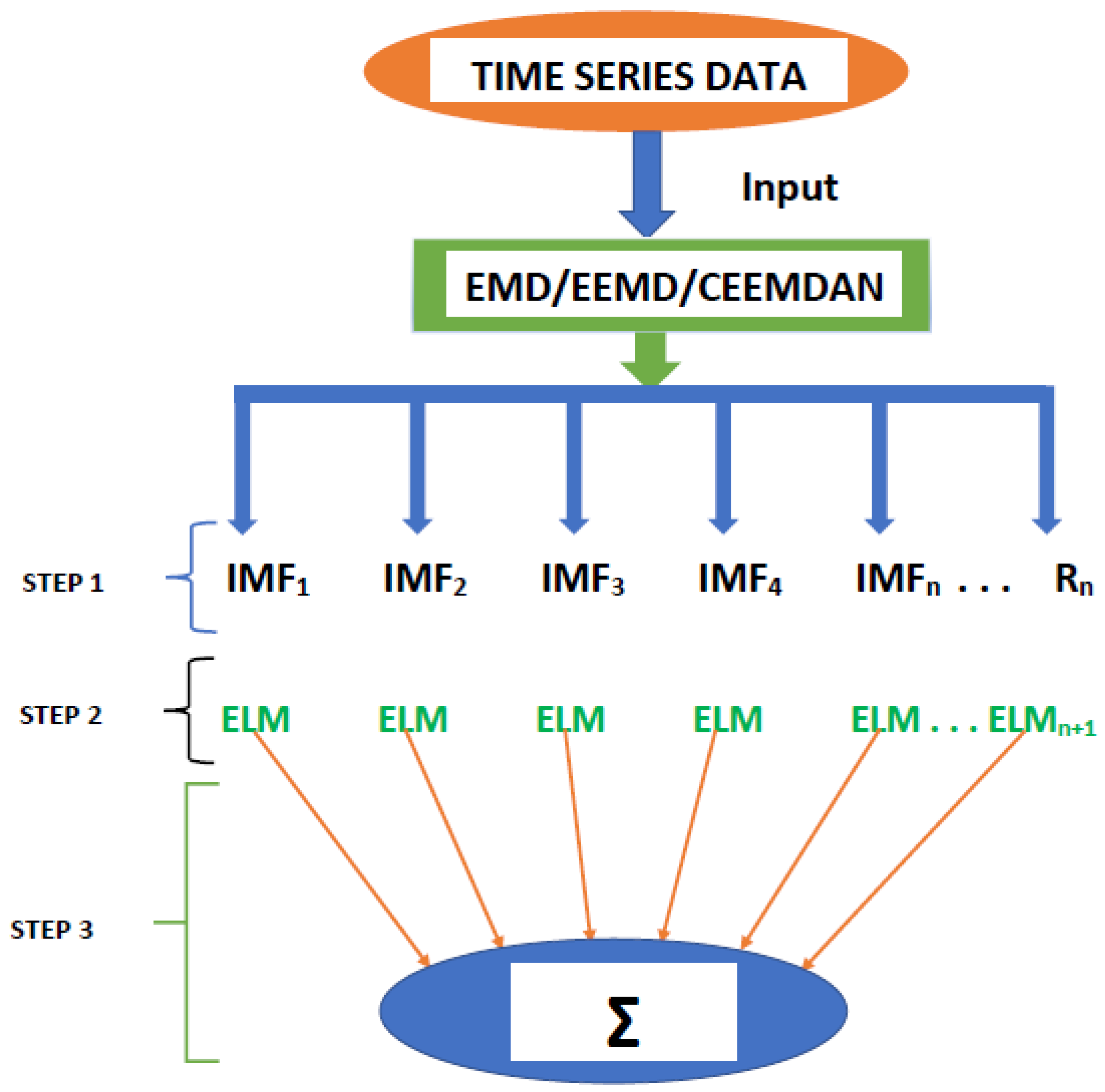
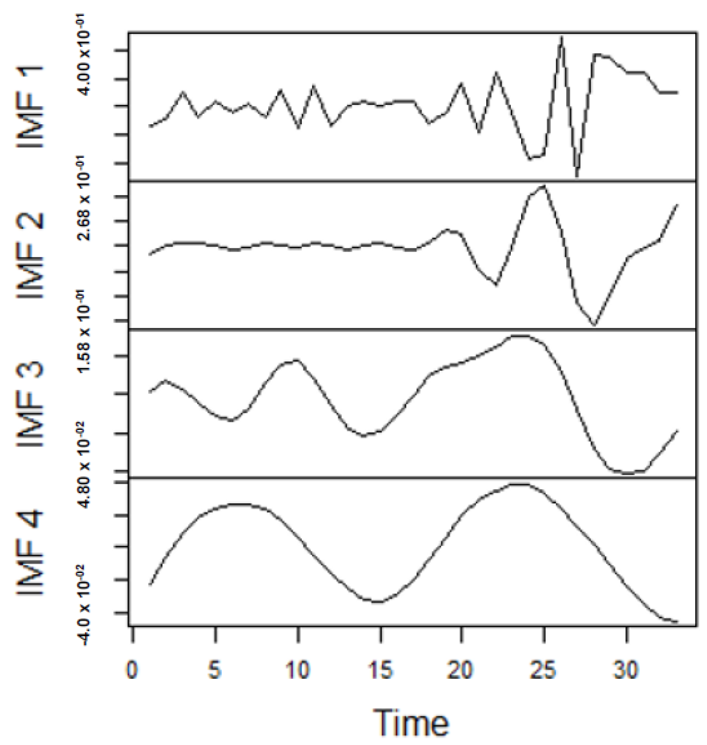
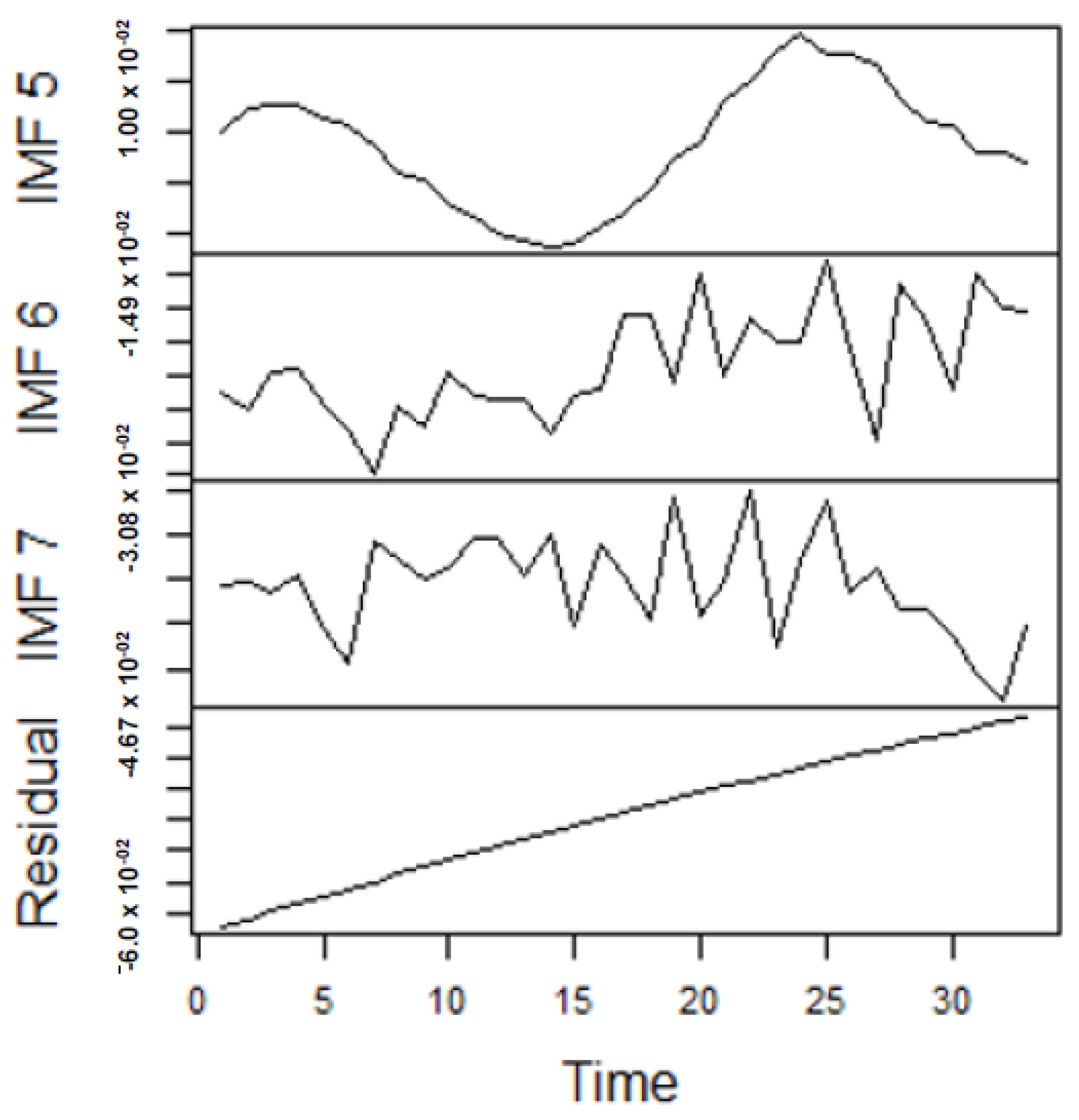
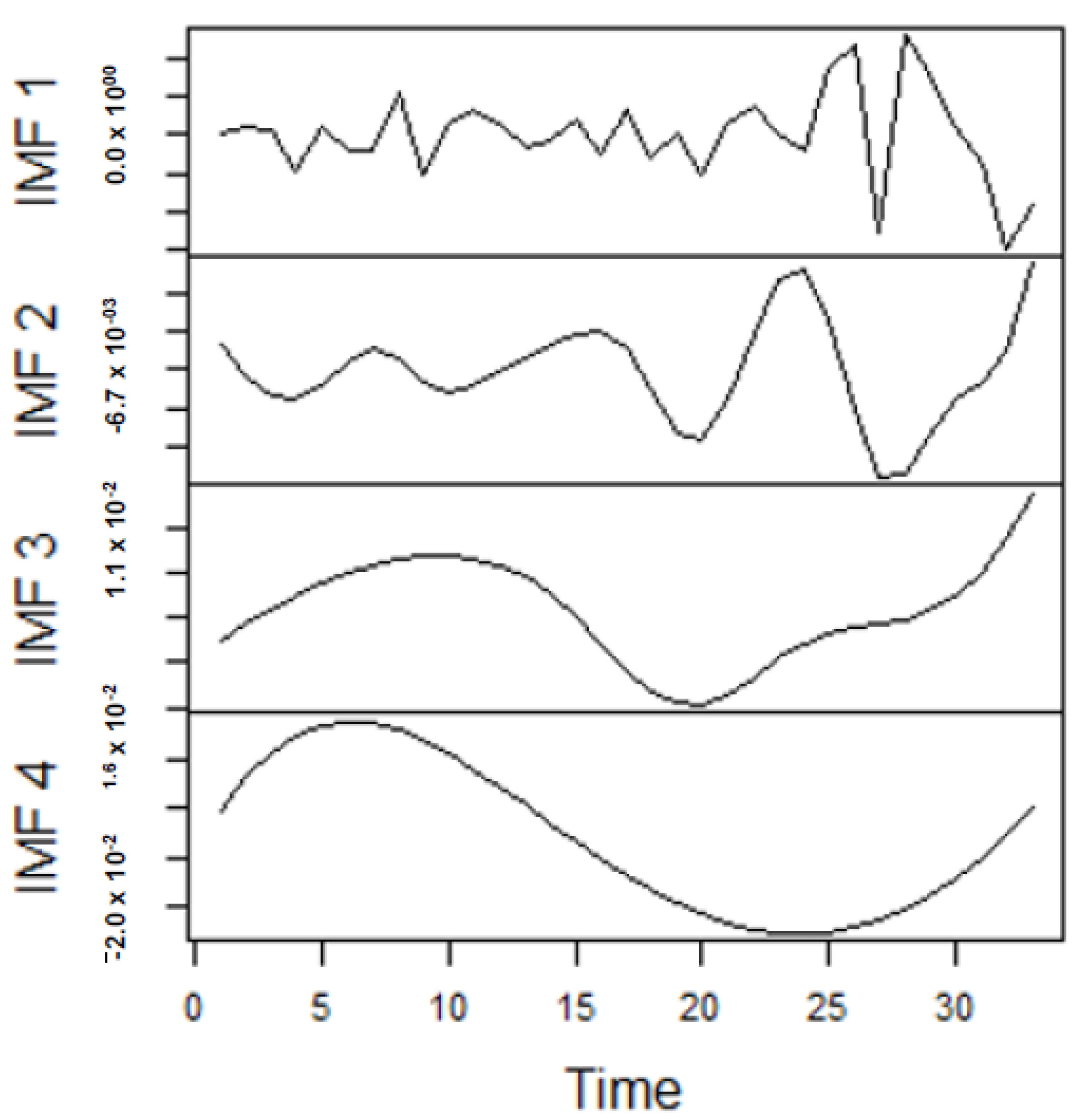
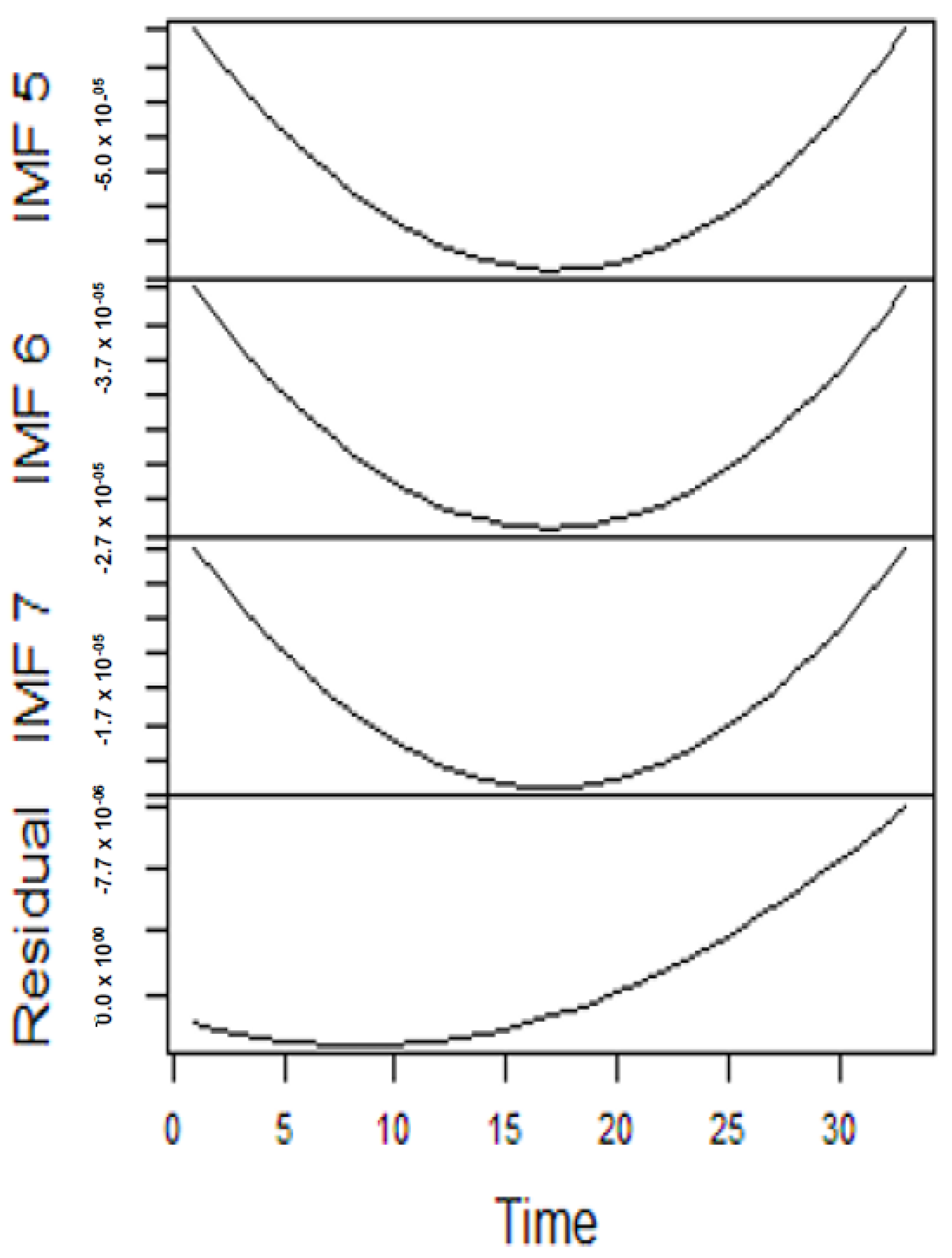
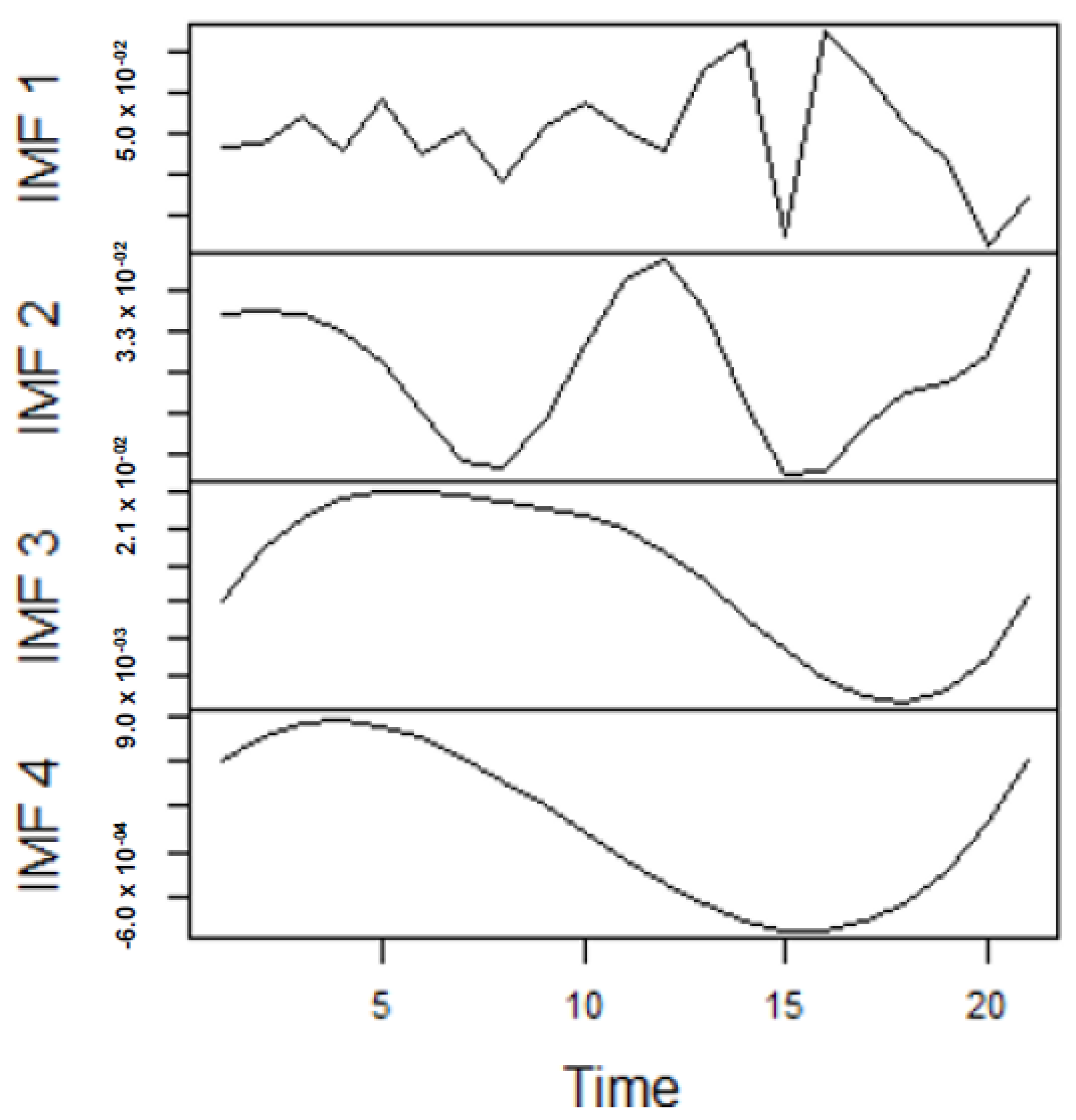
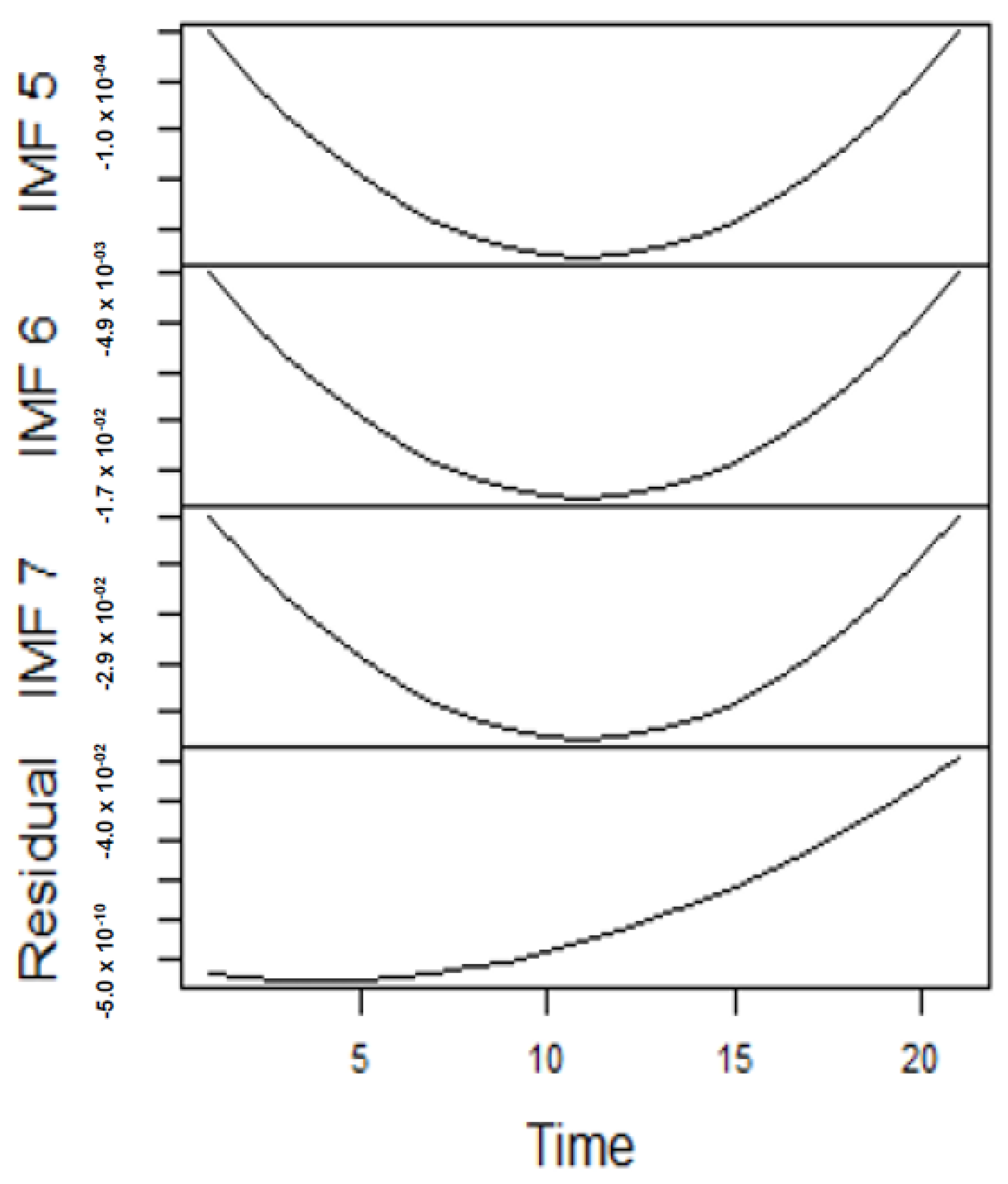
As earlier mentioned, the performance of the EEMD is worsened by some of the IMFs. However, this situation is overcome by the CEEMDAN-ELM, which results in fewer IMFs. Considering this, employing the CEEMDAN-ELM, we conduct various forecasting activities that result in a combination of forecast values of all individual IMFs. An example of this IMFs decomposition for UGAS and JGAS based on CEEMDAN-ELM in the pre-COVID era and stressful paradigm are reported in Figure 5, Figure 6, Figure 7 and Figure 8. 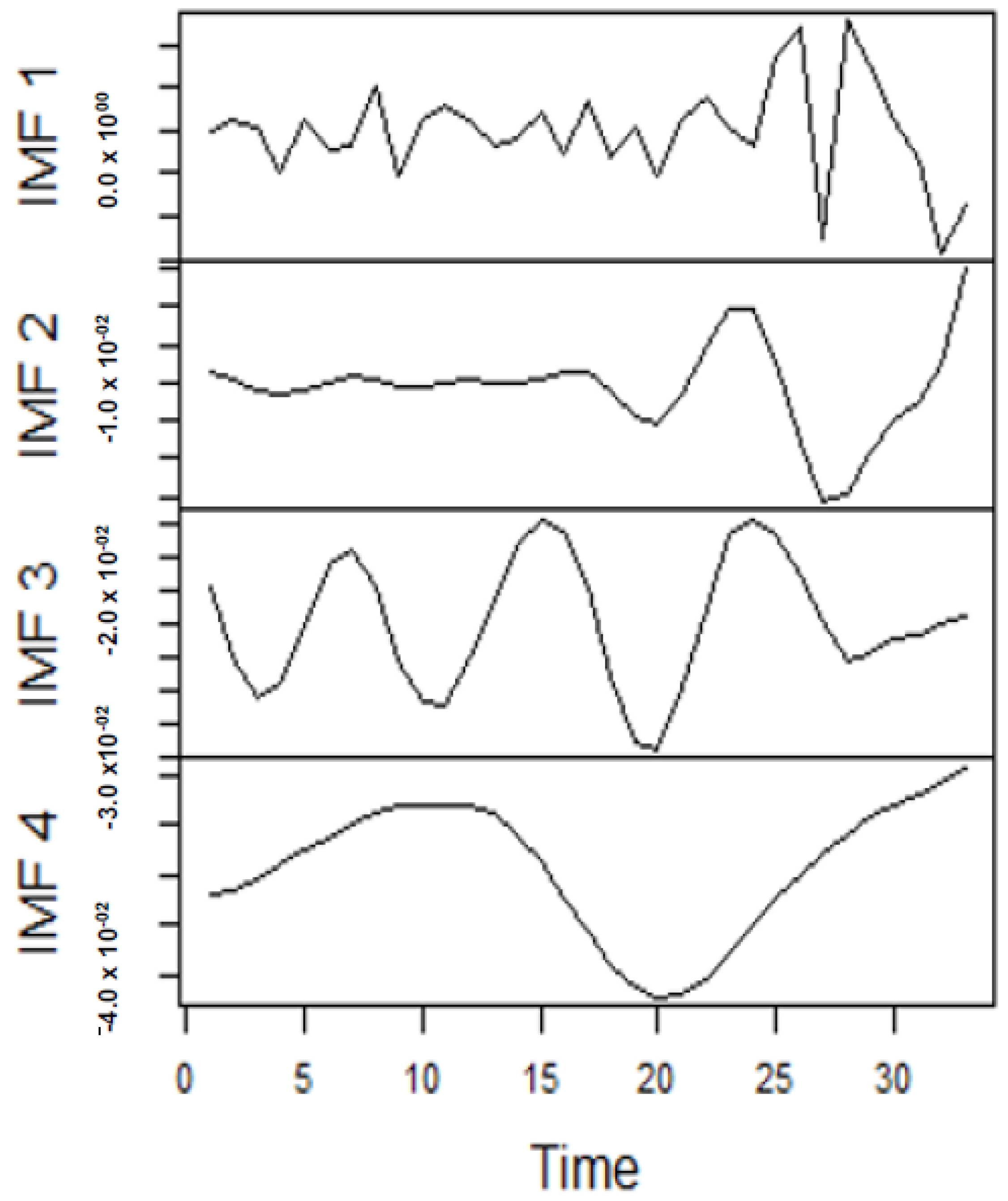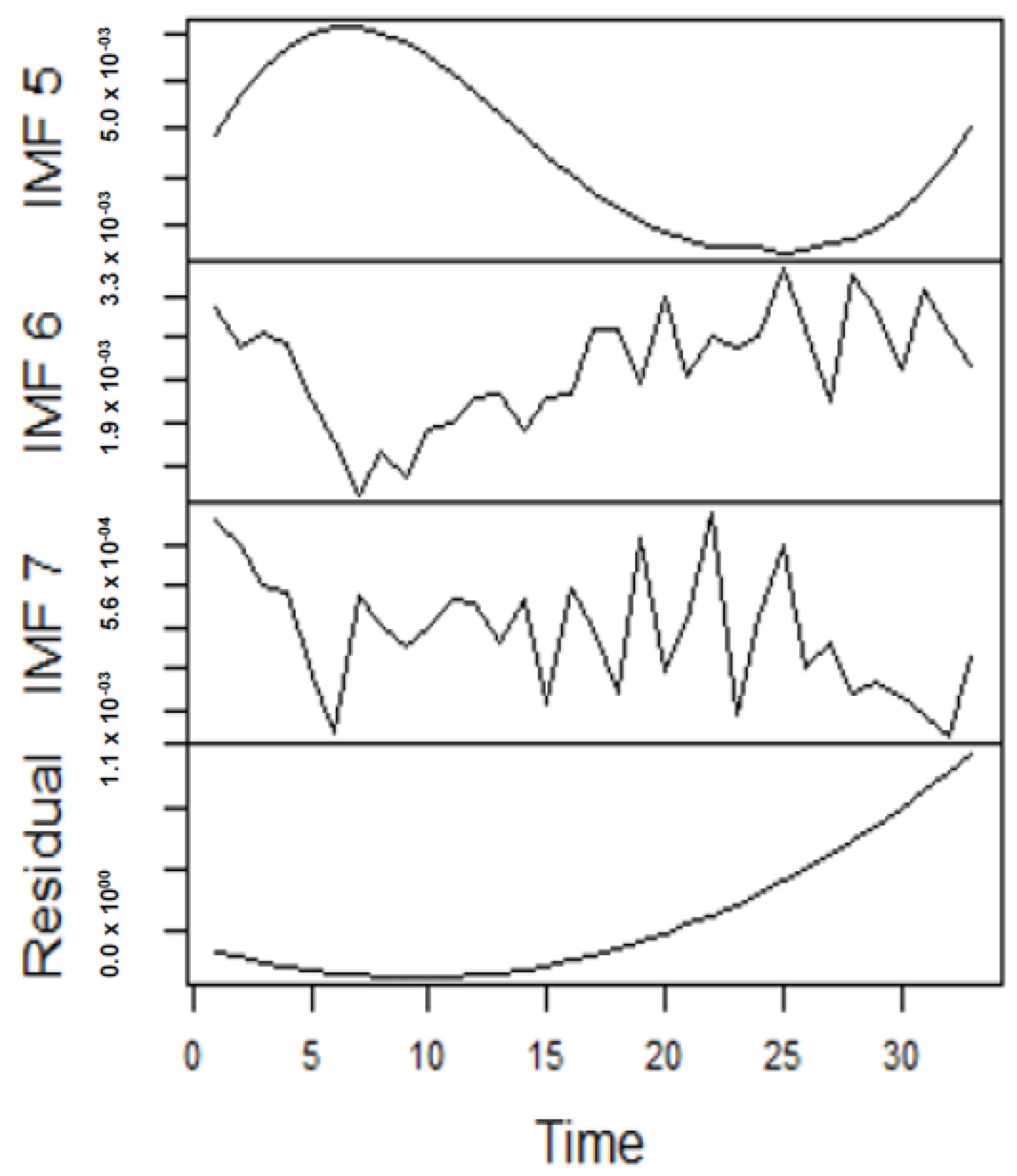Figure 5 and Figure 6 forms a complete set, however, it has been split for clarity of display. A similar situation applies to Figure 7 and Figure 8.

On the other hand, the EEMD seeks to reduce the change of mode mixing, which is an improvement on EMD as already discussed. Hence, extending this to extreme learning machines does lead to an improved forecasting performance. From this viewpoint, of forecasting the generated IMFs, we deduce the combination of forecast values for all individual IMFs, which are reported in Table 4 and Table 5. In consequence, we employ the EMD-based ELM in a similar framework, which entails decomposing the original series followed by the application of ELM to forecast the individual IMFs generated and finally deducing the combined forecast. In effect, the accuracy of these forecasts is derived based on the individual model-specific framework, that is, for the EMD-ELM, we have the Mean Absolute Error (MAE) for EMD-ELM model (MAE-EMD-ELM), the Mean Absolute Percentage Error (MAPE) for EMD-ELM model (MAPE-EMD-ELM), and Root Mean Square Error (RMSE) for EMD-ELM model (RMSE-EMD-ELM).

From the lenses of the sifting process, we obtain 7 IMFs in addition to one residual for all the energy price series. It is worth noting that all the IMFs deduced ranges from the highest frequency to the lowest frequency. The residuals show a varying movement toward the long-term average. Using our research methodology, the forecast experiment conducted using the energy commodity time series data exhibit varying dynamics. 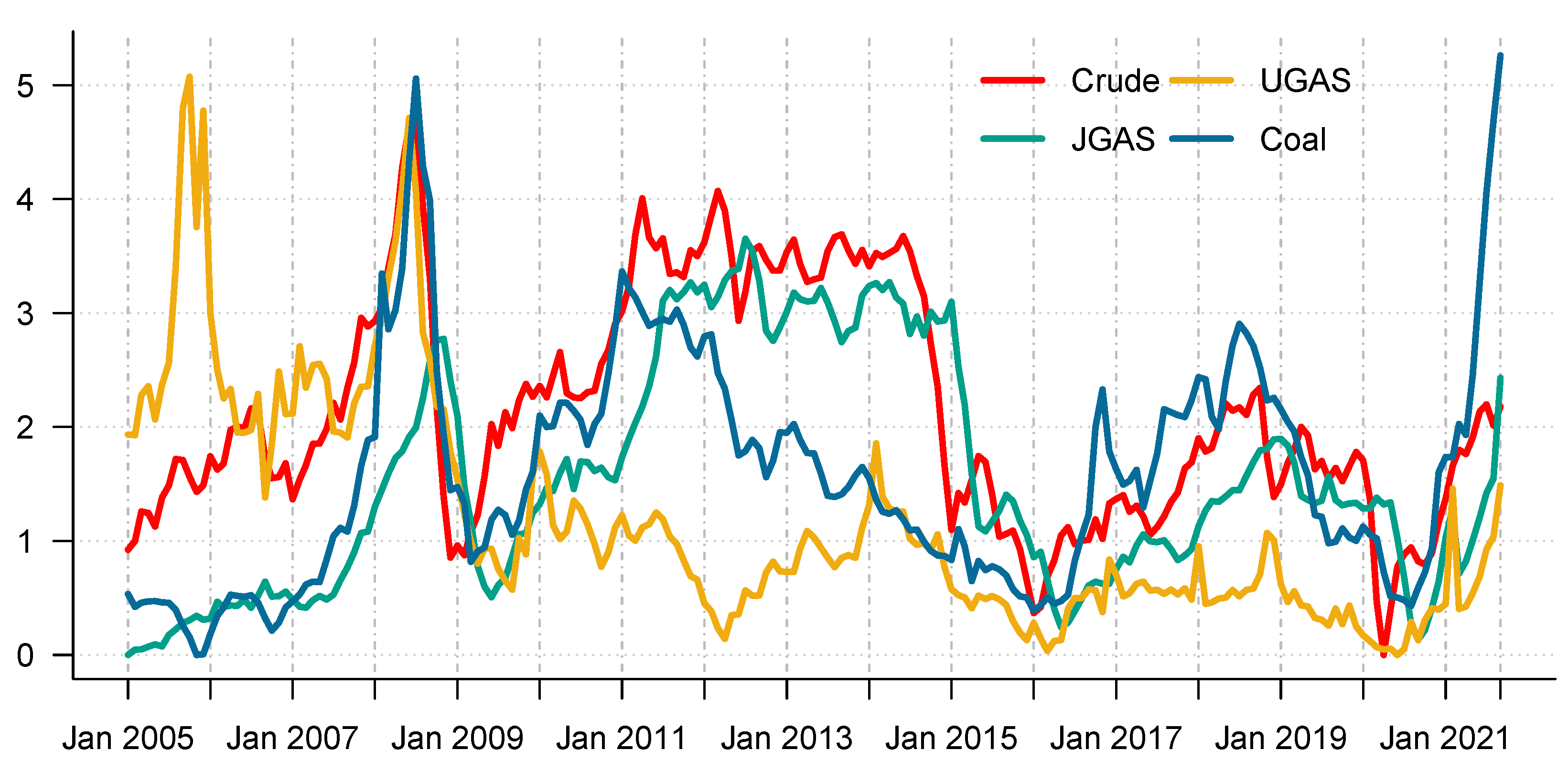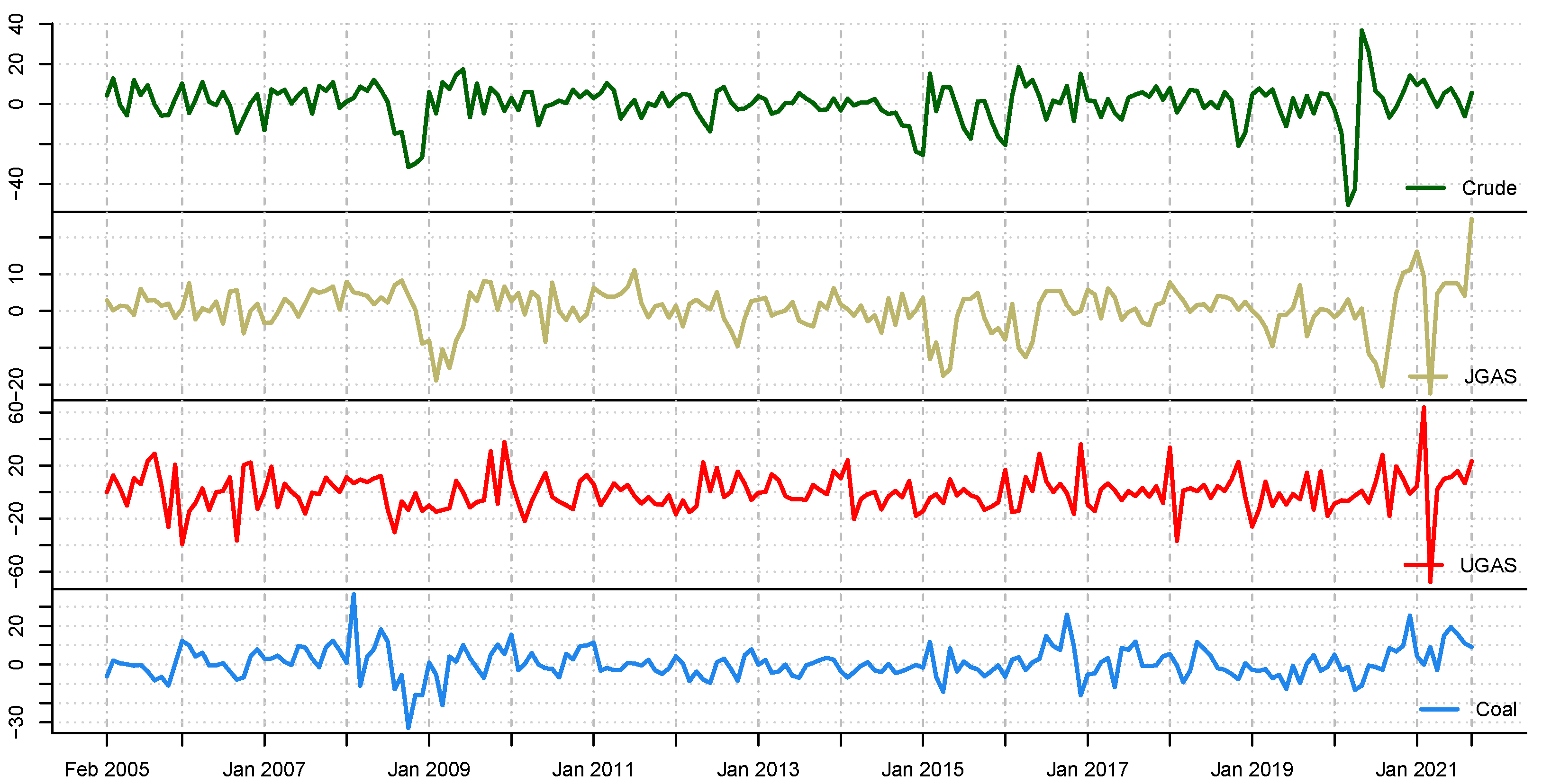After the decomposition, as illustrated, for example in Figure 9, Figure 10, Figure 11 and Figure 12 (Figure 9 is a continuation of Figure 10 and similarly Figure 11 is again continuation of Figure 12. We split the diagrams for clarity of the graphical display, which depicts the IMFs and the residuals produced), the ELM coupled with the iterated strategy is used to forecast the extracted IMFs and the remaining components. In consequence, the prediction outcome of a 12-month horizon is considered for all the energy commodity series among the decomposition-based extreme learning machines in relation to the benchmark model. For each scenario, we separate the data into two parts, which are the training and the test data set. Specifically, for the first scenario, which depicts the pre-COVID period, we consider January 2005 to December 2018 as in-sample data and January 2019 to December 2019 as the out-of-sample data. Shifting the aforementioned dataset over 12 months leads to the second scenario, which has January 2005 to December 2019 as the in-sample data, and January 2020 to December 2020 as the out of sample data with the specific purpose of comparing normal times, indicative of the non-COVID period and the COVID-period itself.

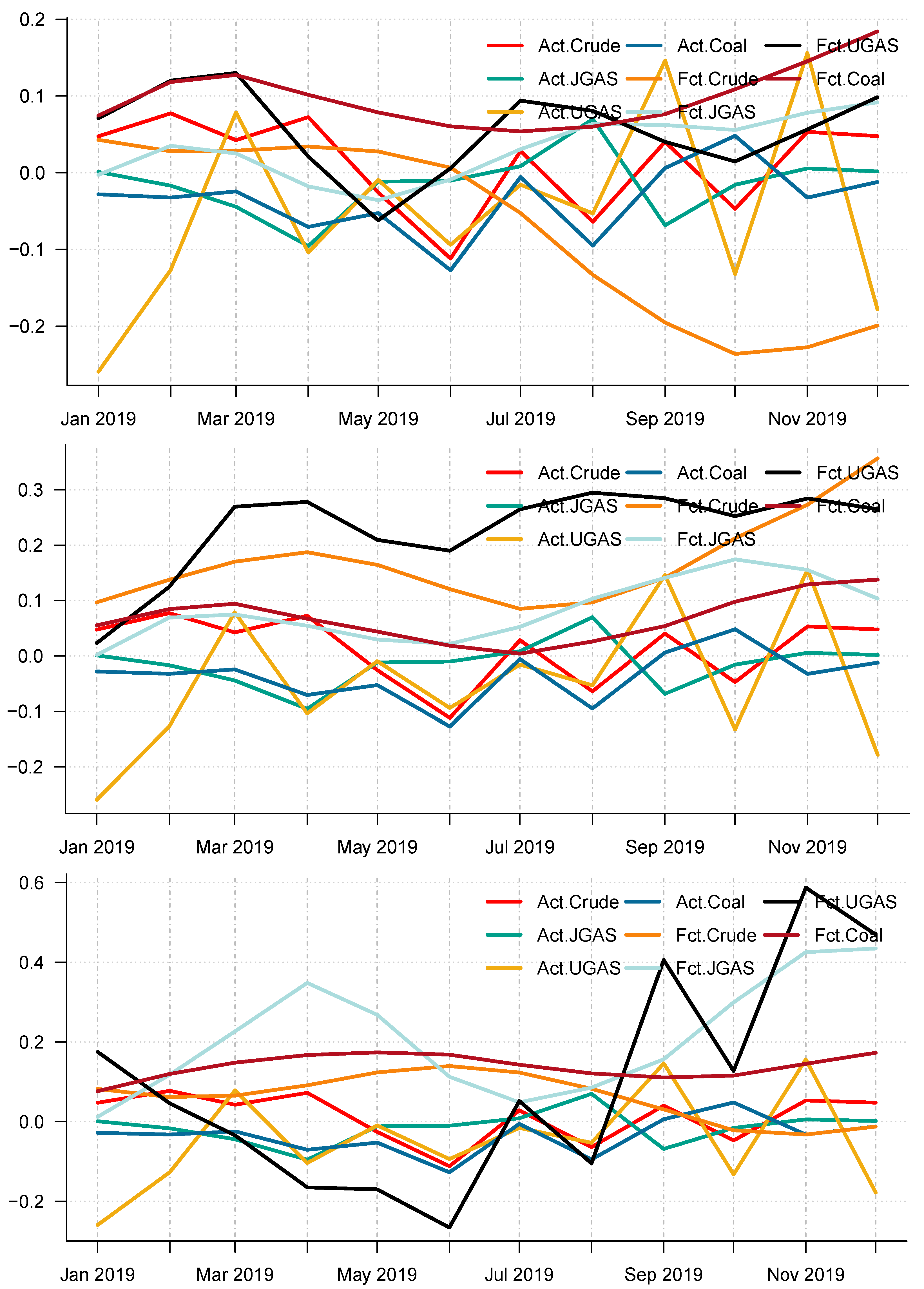
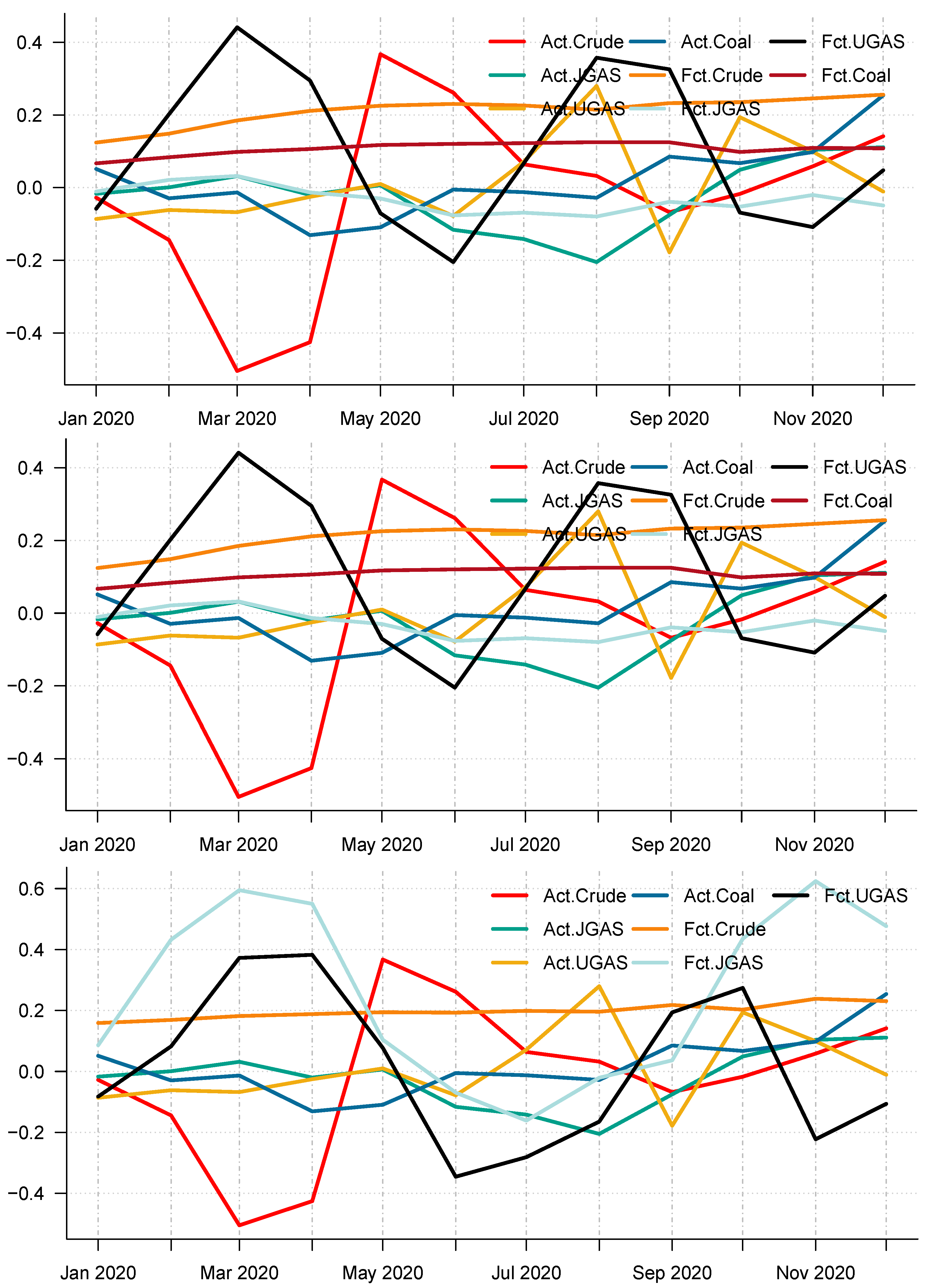
Moreover, using the different accuracy forecast measures, it is obvious that CEEMDAN-ELM is best suitable for forecasting UGAS in the pre-crisis periods based on model-specific forecasting measures, which can be inferred from Table 4 with the combined forecast final values for all the IMFs reported in Panel A of Figure 13. However, this is not the case during the COVID-19 outbreak. The CEEMDAN-ELM provides the best forecast for Coal instead in this period. On the other hand, the EEMD-ELM provides an accurate forecast for JGAS in the pre-COVID-19 era whereas the crude oil is the best forecast using the EMD-ELM based on all the three forecasts accuracy measures. One interesting observation is that coal, crude oil, and JGAS strives with EEMD-ELM and appears to be useful for forecasting purposes during the crisis period. Unlike the normal era, which is the period before the COVID-19, coal could not survive the test for EMD-ELM during the stressful periods, which is in our case; the COVID-19 dispensation. All in all, it is evident that EEMD-ELM exhibit some degree of resilience in providing an accurate forecast in both paradigms. The plot of the actual series and the forecast series also reveals the dynamics of the predictions of the different modeling frameworks See Figure 13 and Figure 14 for an overview. Figure 13 and Figure 14 display the forecast of the various models. In effect, a complete overview of the two eras shows that the models utilized are capable of capturing various dynamics in the data. On the whole, we consider a 12-month forecast horizon for the two scenarios under consideration. The scenarios described above are observed based solely on the decomposition-based extreme learning machine models. However, the above dynamics changed with the introduction of a benchmark model; namely the autoregressive integrated moving average model (ARIMA). The complete model framework is depicted in ARIMA ($p,d,q$), where p is the order of the autoregressive part, d, represents the number of differencing required to make the time series stationary, and q depicts the order of the moving average part.

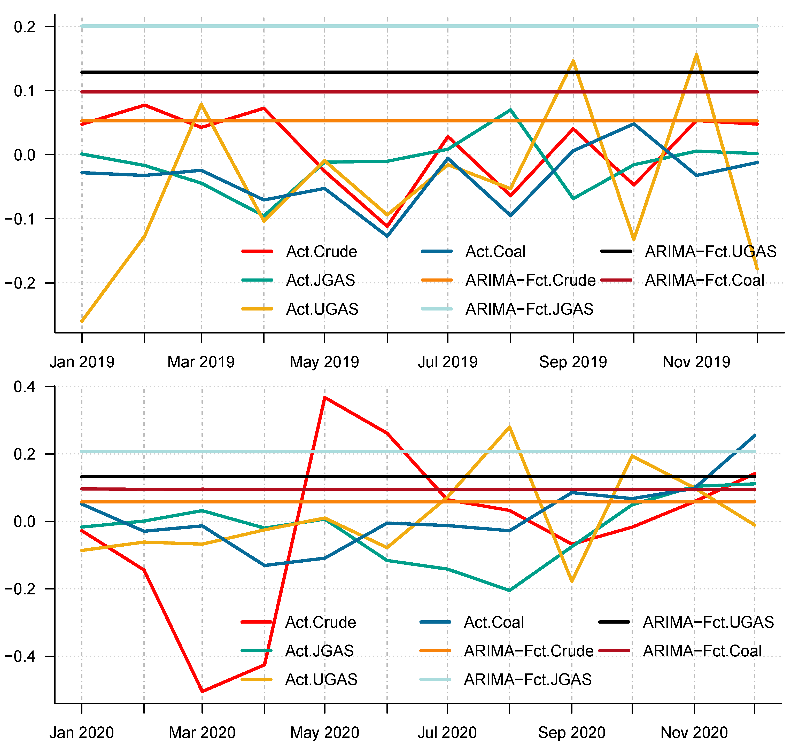
In particular, we employ the autoregressive integrated moving average, which is a commonly used technique to fit most time series data and for forecasting purposes. After all the necessary checks and balances in terms of the autocorrelation function (ACF) and the partial autocorrelation function (PACF), the series shows that AR (1) is appropriate to use on the energy commodity time series data because the ACF tail off and the PACF cuts in the first lag. As such, we apply the ARIMA (1,1,0) to model the energy commodity price changes, whose forecasts could be observed in the different panels of Figure 13 and Figure 14. Surprisingly, comparing the benchmark model with the decomposition-based extreme learning machine models based on model-specific forecast error measures (i.e. minimum values of ARIMA-MAE and ARIMA-RMSE) shows that the ARIMA model outperforms the other models in favor of the JGAS and the UGAS markets in both two scenarios, which the before COVID-19 and during COVID-19 periods.

Furthermore, to check the superiority of our modeling framework, this paper utilizes the model confidence set (MCS) pioneered by [40] to select a set of superior models in the scenarios under consideration (A package in R to evaluate the MCS has been written by [40]). A MCS is a representation of the construction of a set of models such that it selects only the best models with a given level of confidence. The MCS accommodates various limitations of the data, in which case, if the data is not informative, it yields an MCS with many models. Otherwise, if it is informative enough, it yields an MCS with only a few models. It is worth noting that the MCS method does not assume that a particular model is the true model and therefore can be applied without loss of generalization. We, therefore, apply the MCS to our models including the benchmark model. One characterization of the MCS is that a model is discarded only if it is found to be significantly inferior to another model. A competitive advantage of the MCS in comparison with other selection procedures is that the MCS acknowledges the limits to the information contained in the data. In effect, the MCS procedure yields a set of models that summarizes key sample information. The differences in the forecasting performances of all these approaches have been compared and tested by means of the MCS. The details of the outcome of the MCS evaluation is reported for the two scenarios in

Table 6. Model confidence set: Resulting superiority set of models in 2019.

Energy Assets	Model	Ranking
Crude	CEEMDAN–ELM	1.000
JGAS	CEEMDAN–ELM	1.000
UGAS	CEEMDAN–ELM	1.000
	EEMD–ELM	2.000
Coal	EEMD–ELM	1.000

and

Table 7. Model confidence set: Resulting superiority set of models in 2020.

Energy Asset	Model	Ranking
Crude	EEMD–ELM_Crude	2.000
	EMD–ELM	1.000
JGas	CEEMDAN–ELM	1.000
	EEMD–ELM	2.000
UGas	CEEMDAN–ELM	2.000
	EEMD–ELM	3.000
	EMD–ELM	1.000
Coal	CEEMDAN–ELM	1.000

respectively. Some important results emerge. Based on each commodity, we have rankings that depict the model that performs best. For example, in 2019, CEEMDAN-ELM favors crude oil, JGAS, and UGAS only, whilst the MCS captures UGAS and Coal for EEMD-ELM. These dynamics, however, changed in 2020 with EMD-ELM featuring in the MCS for all the commodities, except Coal, which resulted in CEEMDAN-ELM after the MCS evaluation. One unique observation based on the MCS is that all the decomposition-based extreme learning machine framework is captured by the MCS in favor of UGAS. Nonetheless, it is worth noting that the ARIMA is completely absent from the MCS, which already shows that the decomposition-based extreme learning machines outperform the ARIMA modeling framework. In this case, the decomposition-based extreme learning machine models appear to be the more superior models. The inferiority of the benchmark is due to the fact that it cannot capture the non-linearity (see Figure 15 for a reference) as compared to the other three models, which are the CEEMDAN-ELM, EEMD-ELM, and the EMD-ELM models that exhibit various non-linear dynamics. This is evident in the pre-COVID-19 era as well as during the COVID-19 dispensation.

An alternative to the MCS is the possibility of using a statistical test that distinguishes between the predictive accuracy of two sets of forecasts. This is based on the principles of the Kolmogorov-Smirnov (KS) test, which is referred to as the KS Predictive Accuracy (KSPA) test. As indicated by [41], a small number of observations result in an accurate KSPA test establishing a statistically significant difference between the forecasts. The KSPA test comes along with another competitive advantage in that it can compare the empirical cumulative distribution function of the errors from two forecasting models because of the nature of these computations. On the other hand, it is non-parametric, which implies that it makes no assumption based on the characterizations of the underlying errors. In a similar viewpoint, since our forecast horizon is 12-months, employing the KSPA test resulted in a statistically significant difference between the pairwise comparisons. 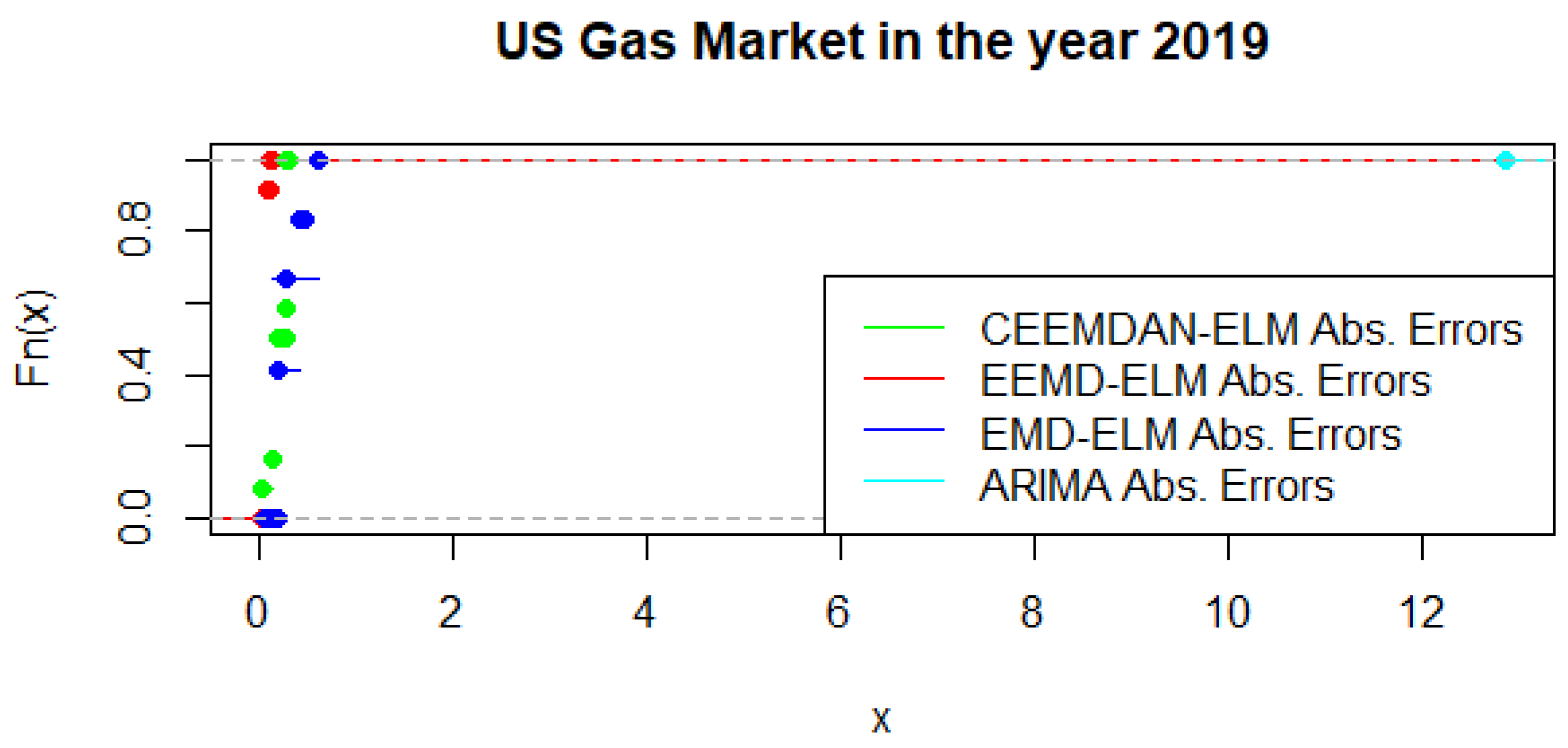However, in a multi-commodity framework, these comparisons become a daunting task as pointed out by [41], hence we propose that the MCS might be a suitable choice in this sense. Nonetheless, with some extensions of the KSPA to a multivariate fashion, it might be an ideal choice for these types of analysis. 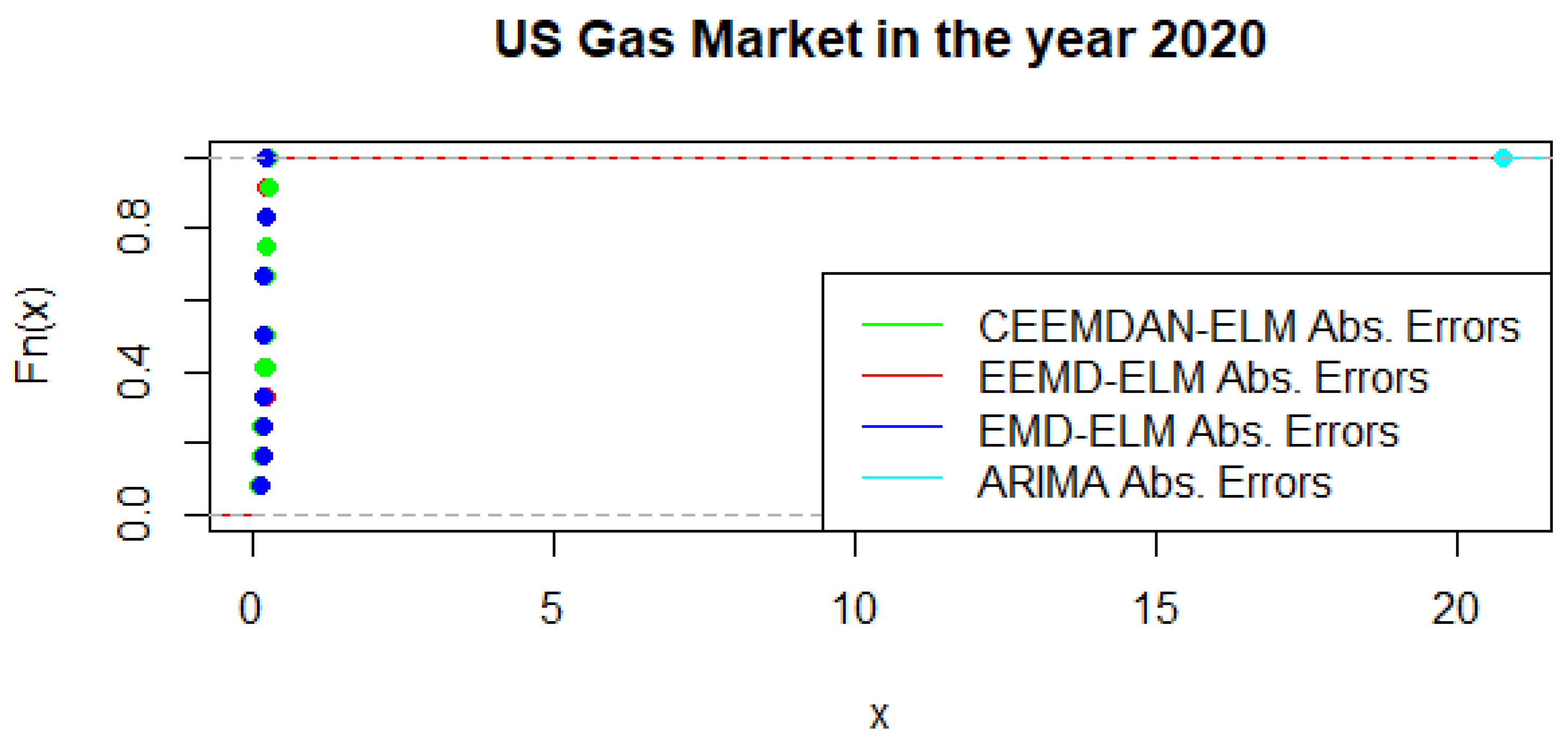As an illustration, Figure 16 present a graphical display of the cumulative distribution function of UGAS forecast errors, which shows various variation among the different modeling framework. CEEMDAN-ELM followed by EEMD-ELM represent better random variations in the sense that the smaller the error deviation the better the forecast accuracy; a result which is not far from the relative accomplishment of the MCS comparatively. Nonetheless, a slight variation could be observed in the US gas market in 2020 as displayed in Figure 17. This is evident between EMD-ELM and EEMD-ELM as well as between CEEMDAN-ELM and EEMD-ELM errors. However, the ARIMA errors exhibit the largest variations in 2019 and 2020.

6. Conclusions

This paper has successfully proposed and employed the extended empirical mode decomposition useful for the time-frequency analysis method, which can adapt to various non-stationarity signals and thus enhance forecasting performance in this era of the information age, where there is the prevalence of huge volumes of data in the energy sector that are hard to manage. In particular, variants of ensemble empirical mode decomposition-based extreme learning machines namely: (i) Complete Ensemble Empirical Mode Decomposition with Adaptive Noise-based ELM Model, (ii) Ensemble Empirical Mode Decomposition-based ELM Model (EEMD-ELM) and (iii) Empirical Mode Decomposition-based ELM Model (EMD-ELM) have been utilized in the spirit of soft computing and artificial intelligence to analyze multi-commodity time series via decomposition methods, which exhibit relevant features for volatility forecasting.

In addition, the ARIMA model has been introduced as a benchmark in the two scenarios, which has revealed that the decomposition-based extreme learning machine outperforms the benchmark model, which explains the ability of the combined forecasting models to capture various dynamics such as non-stationarity, non-linearity among others as compared to other univariate benchmark model based on their predictive accuracy abilities. To this extent, we perform robustness checks to test the superiority of the models by using the Model confidence set and the Kolmogorov-Smirnov Predictive Accuracy (KSPA) test. We find that while both models are suitable and serve the same purpose of detecting the superiority of the models, the MCS is more preferred to the KPSA test due to its pairwise test limitations. Nonetheless, a quick illustration shows that the results might not be quite disparate from each other. Overall, our findings provide model-specific forecast accuracy measures, which reveal that CEEMDAN-ELM, EEMD-ELM, and EMD-ELM provide the best forecast for US gas, Japan gas, crude oil, respectively, before the outbreak of COVID-19. Furthermore, we obtain mixed results during the COVID-19 outbreak. In consequence, EEMD-ELM shows resilience in providing an accurate forecast for Japanese gas in both non-stressful and stressful periods. The foregoing showcases the situation when the comparison is based on the decomposition-based extreme learning machines only. On the other hand, a slight change in dynamics is observed with the introduction of a benchmark, where the ARIMA model outperforms the decomposition-based extreme learning machine models in the case of the Japan gas and the US gas markets.

However, applying the Model confidence set in the pre-COVID era, CEEMDAN-ELM shows persistence and superiority in accurately forecasting Crude oil, JGAS, and UGAS. Nonetheless, this paradigm changed in the COVID-era, which saw CEEMDAN-ELM favoring JGAS, UGAS, and coal with different rankings via the Model confidence set evaluation methods. Overall, all decomposition-based extreme learning machines are superior to the benchmark model. Our modeling framework provides promising tools in this era of big data that have the potential to aid better and fact-based decision making and hence, are relevant for policymakers and various actors in the commodity markets and provide a platform for consideration in other commodity markets. This study is not without limitations. One of the shortcomings of this study is that various underlying factors influence prices and hence an extension to capture these underlying factors might be a consideration for future research, specifically, in a multivariate fashion. Moreover, this study is limited to point forecasting, hence, interval forecasting might be considered for future research, which could be of great value to various practitioners in the energy commodity market and beyond.

References

1. Fianu, E.S. Artificial Intelligence Meets Computational Intelligence: Multi-Commodity Price Volatility Accuracy Forecast with Variants of Markov-Switching-GARCH–Type–Extreme Learning Machines Hybridization Framework. 2022. Available online: https://ssrn.com/abstract=4101277 (accessed on 27 February 2022).
2. Huang, N.E.; Shen, Z.; Long, S.R.; Wu, M.C.; Shih, H.H.; Zheng, Q.; Yen, N.-C.; Tung, C.C.; Liu, H.H. The empirical mode decomposition and the hilbert spectrum for nonlinear and non-stationary time series analysis. Proc. R. Soc. Lond. Ser. A Math. Phys. Eng. Sci. 1971, 454, 903–995. [Google Scholar] [CrossRef]
3. Huang, N.E. New method for nonlinear and nonstationary time series analysis: Empirical mode decomposition and hilbert spectral analysis. In Wavelet Applications VII; International Society for Optics and Photonics: Bellingham, WA, USA, 2000; Volume 4056, pp. 197–209. [Google Scholar]
4. Huang, N.E.; Wu, M.-L.C.; Long, S.R.; Shen, S.S.; Qu, W.; Gloersen, P.; Fan, K.L. A confidence limit for the empirical mode decomposition and hilbert spectral analysis. Proc. R. Soc. Lond. Ser. A Math. Phys. Eng. Sci. 2003, 459, 2317–2345. [Google Scholar] [CrossRef]
5. Ismail, D.; Lazure, K.B.P.; Puillat, I. Advanced spectral analysis and cross correlation based on the empirical mode decomposition: Application to the environmental time series. IEEE Geosci. Remote Sens. Lett. 2015, 12, 1968–1972. [Google Scholar] [CrossRef]
6. Petropoulos, F.; Apiletti, D.; Assimakopoulos, V.; Babai, M.Z.; Barrow, D.K.; Taieb, S.B.; Bergmeir, C.; Bessa, R.J.; Bijak, J.; Boylan, J.E. Forecasting: Theory and practice. Int. J. Forecast 2022, 196, 116630. [Google Scholar] [CrossRef]
7. Mannes, A.E.; Soll, J.B.; Larrick, R. P The wisdom of select crowds. J. Personal. Soc. Psychol. 2014, 276, 1–10. [Google Scholar] [CrossRef]
8. Hong, M.; Sanjay, R.; Wang, T.; Yang, D. Influential factors in crude oil price forecasting. Energy Econ. 2017, 68, 77–88. [Google Scholar]
9. Jamil, R. Hydroelectricity consumption forecast for Pakistan using ARIMA modeling and supply-demand analysis for the year 2030. Renew. Energy 2020, 107, 1–10. [Google Scholar] [CrossRef]
10. Qian, Z.; Pei, Y.; Zareipour, H.; Chen, N. A review and discussion of decomposition-based hybrid models for wind energy forecasting applications. Appl. Energy 2019, 68, 77–88. [Google Scholar] [CrossRef]
11. Yu, L.; Wang, S.; Lai, K.K. Forecasting crude oil price with an emd-based neural network ensemble learning paradigm. Energy Econ. 2008, 30, 2623–2635. [Google Scholar] [CrossRef]
12. Parida, M.; Behera, M.K.; Nayak, N. Combined EMD-ELM and OS-ELM techniques based on feed-forward networks for PV power forecasting. In Proceedings of the IEEE 2018 Technologies for Smart-City Energy Security and Power (ICSESP), Bhubaneswar, India, 28–30 March 2018; pp. 1–6. [Google Scholar]
13. He, K.; Yu, L.; Lai, K.K. Crude oil price analysis and forecasting using wavelet decomposed ensemble model. Energy 2012, 46, 564–574. [Google Scholar] [CrossRef]
14. Yu, L.; Zhao, Y.; Tang, L. A compressed sensing based ai learning paradigm for crude oil price forecasting. Energy Econ. 2014, 46, 236–245. [Google Scholar] [CrossRef]
15. Tang, L.; Dai, W.; Yu, L.; Wang, S. A novel CEEMD-based EELM ensemble learning paradigm for crude oil price forecasting. Int. J. Inf. Technol. Decis. 2015, 14, 141–169. [Google Scholar] [CrossRef]
16. Tang, L.; Lv, H.; Yu, L. An EEMD-based multi-scale fuzzy entropy approach for complexity analysis in clean energy markets. Appl. Soft Comput. 2017, 56, 124–133. [Google Scholar] [CrossRef]
17. Junior, P.O.; Tiwari, A.K.; Padhan, H.; Alagidede, I. Analysis of EEMD-based quantile-in-quantile approach on spot-futures prices of energy and precious metals in india. Resour. Policy 2020, 68, 101731. [Google Scholar] [CrossRef]
18. Yan, B.; Aasma, M. A novel deep learning framework: Prediction and analysis of financial time series using CEEMD and LSTM. Expert Syst. Appl. 2020, 159, 113609. [Google Scholar]
19. Niu, D.; Wang, K.; Sun, L.; Wu, J.; Xu, X. Short-term photovoltaic power generation forecasting based on random forest feature selection and CEEMD: A case study. Appl. Soft Comput. 2020, 93, 106389. [Google Scholar] [CrossRef]
20. Wu, J.; Chen, Y.; Zhou, T.; Li, T. An adaptive hybrid learning paradigm integrating CEEMD, ARIMA and SBL for crude oil price forecasting. Energies 2019, 12, 1239. [Google Scholar] [CrossRef]
21. Gaci, S. A new ensemble empirical mode decomposition (EEMD) de-noising method for seismic signals. Energy Procedia 2016, 97, 84–91. [Google Scholar] [CrossRef]
22. Devi, A.S.; Maragatham, G.; Boopathi, K.; Rangaraj, A. Hourly day-ahead wind power forecasting with the EEMD-CSO-LSTM-EFG deep learning technique. Soft Comput. 2020, 24, 12391–12411. [Google Scholar] [CrossRef]
23. Chen, Y.; Dong, Z.; Wang, Y.; Su, J.; Han, Z.; Zhou, D.; Zhang, K.; Zhao, Y.; Bao, Y. Short-term wind speed predicting framework based on EEMD-GA-LSTM method under large scaled wind history. Energy Convers. Manag. 2021, 227, 113559. [Google Scholar]
24. Li, J.; Jiang, X.; Shao, L.; Liu, H.; Chen, C.; Wang, G.; Du, D. Energy consumption data prediction analysis based on EEMD-ARMA model. In Proceedings of the 2020 IEEE International Conference on Mechatronics and Automation (ICMA), Beijing, China, 13–16 October 2020; pp. 1338–1342. [Google Scholar]
25. Zhang, G.; Zhou, H.; Wang, C.; Xue, H.; Wang, J.; Wan, H. Forecasting time series albedo using narnet based on eemd decomposition. IEEE Trans. Geosci. Remote Sens. 2020, 58, 3544–3557. [Google Scholar] [CrossRef]
26. Zhang, J.-L.; Zhang, Y.-J.; Zhang, L. A novel hybrid method for crude oil price forecasting. Energy Econ. 2015, 49, 649–659. [Google Scholar] [CrossRef]
27. Zhu, B.; Chevallier, J. Carbon price forecasting with a hybrid ARIMA and least squares support vector machines methodology. In Pricing and Forecasting Carbon Markets; Springer: Berlin/Heidelberg, Germany, 2017; pp. 87–107. [Google Scholar]
28. Wu, Z.; Huang, N.E. Ensemble empirical mode decomposition: A noise-assisted data analysis method. Adv. Adapt. Data Anal. 2009, 1, 1–41. [Google Scholar] [CrossRef]
29. Torres, M.E.; Colominas, M.A.; Schlotthauer, G.; Flandrin, P. A complete ensemble empirical mode decomposition with adaptive noise. In Proceedings of the 2011 IEEE International Conference on Acoustics, Speech and Signal Processing (ICASSP), Prague, Czech Republic, 22–27 May 2011; pp. 4144–4147. [Google Scholar]
30. Huang, G.-B.; Wang, D.H.; Lan, Y. Extreme learning machines: A survey. Int. J. Mach. Learn. Cybern. 2011, 2, 107–122. [Google Scholar] [CrossRef]
31. Huang, G.-B.; Zhu, Q.-Y.; Siew, C.-K. Extreme learning machine: A new learning scheme of feed-forward neural networks. In Proceedings of the 2004 IEEE International Joint Conference on Neural Networks, (IEEE Cat. No. 04CH37541), Budapest, Hungary, 25–29 July 2004; Volume 2, pp. 985–990. [Google Scholar]
32. Huang, G.-B.; Zhu, Q.-Y.; Siew, C.-K. Extreme learning machine: Theory and applications. Neurocomputing 2006, 70, 489–501. [Google Scholar] [CrossRef]
33. Rajab, L.; Al-Khatib, T.; Al-Haj, A. Video watermarking algorithms using the svd transform. Eur. J. Sci. Res. 2009, 30, 389–401. [Google Scholar]
34. Hansen, P.R.; Lunde, A. A forecast comparison of volatility models: Does anything beat a garch (1, 1)? J. Appl. Econom. 2005, 20, 873–889. [Google Scholar] [CrossRef]
35. Elliott, G.; Rothenberg, T.J.; Stock, J.H. Efficient Tests for An Autoregressive Unit Root. Econometrica 1996, 64, 813–836. [Google Scholar] [CrossRef]
36. Dutta, A.; Bouri, E.; Uddin, G.S.; Yahya, M. Impact of COVID-19 on global energy markets. In IAEE Energy Forum COVID-19 Issue; IAEE: Cleveland, OH, USA, 2020; Volume 2020, pp. 26–29. [Google Scholar]
37. Karoglou, M. Breaking down the non-normality of stock returns. Eur. J. Financ. 2010, 16, 79–95. [Google Scholar] [CrossRef]
38. Fisher, T.J.; Gallagher, C.M. New weighted portmanteau statistics for time series goodness of fit testing. J. Am. Stat. Assoc. 2012, 107, 777–787. [Google Scholar] [CrossRef]
39. Bouri, E.; Cepni, O.; Gabauer, D.; Gupta, R. Return connectedness across asset classes around the COVID-19 outbreak. Int. Rev. Financ. Anal. 2021, 73, 101646. [Google Scholar] [CrossRef]
40. Hansen, P.R.; Asger, L.; Nason, J.M. The model confidence set. Econometrica 2011, 79, 453–497. [Google Scholar] [CrossRef]
41. Hassani, H.; Sirimal, S.E. A Kolmogorov-Smirnov based test for comparing the predictive accuracy of two sets of forecasts. Econometrics 2015, 3, 590–609. [Google Scholar] [CrossRef]
Figure 1. Flowchart of the procedures used in the hybrid modeling framework.
Forecasting 04 00030 g001
Figure 2. A graphical display of single layer feed-forward network.
Forecasting 04 00030 g002
Figure 3. Time plot of energy commodity series of coal, gas and crude oil between years (2005–2021).
Forecasting 04 00030 g003
Figure 4. A graphical display of the scaled return series of energy asset return price series.
Forecasting 04 00030 g004
Figure 5. Part A: Parts of the IMFs for US gas prices.
Forecasting 04 00030 g005
Figure 6. Part B: The remaining IMFs and residuals for US gas prices.
Forecasting 04 00030 g006
Figure 7. Part A: Part of the IMFs for Japan gas prices.
Forecasting 04 00030 g007
Figure 8. Part B: The remainder of the IMFs and residuals for Japan gas prices.
Forecasting 04 00030 g008
Figure 9. Panel A: Part of the IMFs for Japan gas prices in normal times.
Forecasting 04 00030 g009
Figure 10. Panel B: The remaining IMFs for Japan gas prices in normal times.
Forecasting 04 00030 g010
Figure 11. Panel A: Part of the IMFs for Japan gas prices in stressful periods.
Forecasting 04 00030 g011
Figure 12. Panel B: The subsequent parts of the IMFs and residuals for Japan gas prices in stressful periods.
Forecasting 04 00030 g012
Figure 13. Actual price return series versus price return forecast of (CEEMDAN-ELM, EEMD-ELM, EMD-ELM) hybrid models in 2019. Notably, the abscissa denotes the time in months and the ordinate depicts the forecast errors. (top) Panel A: Actual price return series versus price return forecast of crude oil, gas, and coal in 2019 based on CEEMDAN-ELM. It with noting that the abscissa denotes the time in months and the ordinate depicts the forecast errors. (middle) Panel B: Actual price return series versus price forecast of crude oil, gas, and coal in 2019 based on EEMD-ELM. Also, here, the abscissa denotes the time in months and the ordinate depicts the forecast errors. (bottom) Panel C: Price forecast of crude oil, gas, and coal in 2020 based on EMD-ELM. The x-axis represents time measured in years whilst the y-axis represents the forecast errors.
Forecasting 04 00030 g013
Figure 14. Actual price return series versus price return forecast of (CEEMDAN-ELM, EEMD-ELM, EMD-ELM) hybrid models in 2020. (top) Panel A: Actual price return series versus CEEMDAN-ELM-based price forecast of crude oil, gas, and coal in 2018. (middle) Panel B: Actual price return series versus EEMD-ELM-based price return forecast of crude oil, gas, and coal in 2019. (bottom) Panel C: Actual price return series versus EMD-ELM-based price return forecast of crude oil, gas, and coal in 2020.
Forecasting 04 00030 g014
Figure 15. Actual price return series versus price return ARIMA-based forecast in 2019 and 2020. (top) Panel A: Actual price return series versus ARIMA-based price return forecast of crude oil, gas, and coal in 2019. (bottom) Panel B: Actual price return series versus ARIMA-based price return forecast of crude oil, gas, and coal in 2020.
Forecasting 04 00030 g015
Figure 16. Empirical cumulative distribution function of US gas in 2019.
Forecasting 04 00030 g016
Figure 17. Empirical cumulative distribution function of US gas in 2020.
Forecasting 04 00030 g017