Article

Deep Learning for Demand Forecasting in the Fashion and Apparel Retail Industry

1
The Swedish School of Textiles, University of Boras, S-50190 Boras, Sweden
2
College of Textile and Clothing Engineering, Soochow University, Suzhou 215168, China
*
Author to whom correspondence should be addressed.
Forecasting 2022, 4(2), 565-581; https://doi.org/10.3390/forecast4020031
Submission received: 1 May 2022 / Revised: 7 June 2022 / Accepted: 14 June 2022 / Published: 20 June 2022
(This article belongs to the Special Issue Improved Forecasting through Artificial Intelligence)

Abstract

:
Compared to other industries, fashion apparel retail faces many challenges in predicting future demand for its products with a high degree of precision. Fashion products’ short life cycle, insufficient historical information, highly uncertain market demand, and periodic seasonal trends necessitate the use of models that can contribute to the efficient forecasting of products’ sales and demand. Many researchers have tried to address this problem using conventional forecasting models that predict future demands using historical sales information. While these models predict product demand with fair to moderate accuracy based on previously sold stock, they cannot fully be used for predicting future demands due to the transient behaviour of the fashion industry. This paper proposes an intelligent forecasting system that combines image feature attributes of clothes along with its sales data to predict future demands. The data used for this empirical study is from a European fashion retailer, and it mainly contains sales information on apparel items and their images. The proposed forecast model is built using machine learning and deep learning techniques, which extract essential features of the product images. The model predicts weekly sales of new fashion apparel by finding its best match in the clusters of products that we created using machine learning clustering based on products’ sales profiles and image similarity. The results demonstrated that the performance of our proposed forecast model on the tested or test items is promising, and this model could be effectively used to solve forecasting problems.

1. Introduction

Given the growing number of fashion e-commerce digital platforms, customers can see and choose from a massive number of virtual fashion products merchandised virtually. There has been a dramatic shift in customers’ purchasing behaviour, which is impacted by several factors, such as social media, fashion events, and so forth. Consumers now increasingly prefer to select their products from the immense pool of options and want them to be delivered in a very short time. It is challenging for fashion retailers to fulfil consumer demands in a short time interval [1]. Therefore, it is crucial for fashion apparel retailers to make efficient and quick decisions concerning inventory replenishment in advance based on the forecast of future demand patterns.
Demand forecasting plays a crucial role in managing efficient supply chain operations in the fashion retail industry. Poor forecasting models lead to inefficient management of the stock inventory, obsolescence, and disorderly resource utilisation across the upstream supply chain. Usually, profit-oriented companies are much more concerned about forecasting models as most of their business decisions are made based on the predicted future uncertainties related to product demand and sales. In the fashion apparel industry, a plethora of factors such as different product styles, patterns, designs, short life cycles, fluctuating demands, and extended replenishment lead times lead to flawed or less accurate predictions of future product demand or sales [2,3]. The apparel fashion industry is attempting to develop robust forecast models, which can help improve the overall efficiency in the decision-making related to sourcing as well as sales.
Most of the existing research on fashion supply chain management is devoted to developing advanced models for improving the forecast of demand for fashion apparel items [4,5]. Accurately predicting future sales and demand for fashion products remains a central problem in both industry and academia. To address this challenge, it is imperative to study the complexity of the fashion market and managerial strategies that would allow products to be designed, produced, and delivered on time [6]. The fashion apparel industry has been undergoing significant transitions given factors such as dynamic pricing strategies, inventory management, globalisation, and consumer-centric and technology-oriented product design and manufacturing. In need to overcome complexities arising out of these factors, the fashion industry strives to manage these rapid changes more effectively by adopting an agile supply chain [7,8].
The frequency at which new fashion product arrives in the market is relatively very high. How these new fashion products will spare in the market in terms of sales and demand is often the main focus of decision-makers in the fashion supply chain [9]. Therefore, it becomes a difficult challenge for the fashion retailers to predict the future demand and sale of a newly arrived fashion product amidst various factors such as changing consumer choices, in numerous product types, instability in the market, uncertainty in the supply chain, and poor predictability by week or item. In the era of big data, the fashion apparel retail industry produces a considerable amount of sales and item-related information [10] and, if this is handled effectively using cutting-edge data analytics tools, business performance in the fashion industry could be significantly improved.
In fashion retail management, forecast models for predicting product sales and demand are traditionally applied to historical product data that contains sales information and image data features [9]. However, there is often a lack of historical data for the newly arriving fashion item. In the absence of historical data, predicting future demand and sale of a newly arrived fashion item becomes challenging. Historical product data has two main components: sales data and product image data. Image data entail information about attributes of the item, such as colour, style, pattern, and various other essential features. Historical sales data for building forecasting models are not representative of all the product aspects; therefore, they need to be complemented with additional data such as product image data, social media data, and consumer data to predict the fashion apparel demand. Newly arrived fashion product items may differ from the existing products in many ways; however, there could be many of its similar features, such as colour, size, and style, etc. present in the historical product data that could be extracted, and their impact could be explored for forecast modelling.
This paper addresses the limitations of the classical forecasting system by proposing a novel approach for building an intelligent demand forecasting system using advanced machine learning methods and historical product image data. A complete research workflow is shown in Figure 1, which consists of several steps explained in detail in Section 3.1. Machine learning clustering models are applied to a real historical dataset of fashion products, the outcome of which are the two main clusters of the products based on their historical sales. The newly arrived fashion product item is then matched with these two clusters, and the model predicts which one of these two clusters the newly arrived fashion item belongs to. Our model predicts a new item’s sales based on the nearest match it finds in the two clusters and the associated sales profile of a matched product. The performance of the models evaluated on the test dataset and the results from our study were found to be effective and promising for predicting a new fashion product’s sales.
The rest of the paper is organised as follows: Section 2 presents the literature. The Research Methodology is explained in Section 3. The results are discussed in Section 4. Finally, Section 5 and Section 6 discuss the results of the research study and provides concluding remarks.

2. State-of-the-Art

A number of forecasting methods have been developed and employed in the fashion retail industry over the past few years. Statistical approaches, such as regression modelling, are used in [11] for the sales forecast. Linear time series forecasting models such as ARIMA and Exponential smoothing have been widely used for forecasting short-term as well as long-term sales and demands [12,13], Box and Jenkins methods [14] are popular for demand forecasting. However, these methods have limitations in terms of transforming qualitative features of the data into quantitative ones because sales patterns significantly vary in the fashion retail industry [15]. Linear forecast models suffer from significant limitations such as not capturing the nonlinear relationship between various exogenous variables, outliers, missing data, and nonlinear components that are often present in actual time series data [16].
Machine learning and deep learning models such as the support vector machine [1], neural network [17], and recurrent neural network [2] are among many forecast models that have gained popularity among forecast researchers and practitioners given their ability to overcome the drawbacks of traditional linear forecast models. NN models are considered the most efficient forecasting methods, as they have demonstrated high performance in various studies [18]. In [19], the NN model is used to forecast weekly product demand in German supermarkets, and its forecasting performance was found to be high. In another comparative study by [20], the NN model’s performance for forecasting aggregate retail sales was reported better than traditional linear statistical forecast models, and it was found to have effectively captured the seasonality and dynamic trends in the time series sales data. The backpropagation NN model is one of the NN model variants that was found to have generated a highly accurate forecast of sales profile in [21]. Moreover, the NN model is found to be effective at de-seasonalising time series data in the study by [18] that traditional linear models fail to do. A hybrid model integrating a genetic algorithm and NN forecast model is presented in [22] to improve the sales forecast’s accuracy.
The major shortcoming of traditional linear forecast models, as well as expert algorithms, is that they cannot learn from unstructured data such as text data, social media data, and image data. Product image data analysis can provide valuable insights and can be used for forecasting sales from historical sales data and product image data. Machine learning methods are popular for dealing with various data types, both structured and unstructured data. Image clustering is one of the widely used advanced machine learning techniques that discover similar image features from the image data and categorises them into clusters based on the degree of similarity [23].
Laney and Goes [24] highlight that data mining has gained popularity with the introduction of big data. Data mining and artificial intelligence overcome the problems of the classical approaches to forecasting problems [25,26]. Recently, the growing popularity of deep learning models and their advantages in solving data mining problems over traditional models has attracted more attention from the scientific community from forecasting research [27]. Deep learning has found a plethora of applications in many areas, and significant research has been done on it in the medical [28], transportation [29], electricity [30], and agriculture [31] fields. Sales prediction was performed in various studies, such as [26,31], for different product categories using machine learning methods. In another interesting study by Thomassey [32], clustering and NN are combined to predict long-term fashion sales using historical sales. Significantly, the CNN model has been gaining popularity in image recognition and clustering since 2014 [33].
Given the advances and opportunities of the machine learning methods and the afore-cited limitations of traditional forecast models in the domain of sales forecasting in fashion retailing, we propose a novel approach to combine the deep learning and machine learning clustering algorithm on product image data to build a forecasting model in order to predict the sales of future apparel items.
In our work, we exploit product image data to find the closest match for a newly arrived fashion item by applying the machine image clustering technique and predict its sales profile by projecting the sales profile of its best closest match. This study addresses a challenging decision problem in fashion retail, that is, the prediction of a sales profile for a newly launched fashion product that in principle does not have any previous historical data. We leverage image and sales data of the fashion products, and machine learning techniques to propose a sales forecast approach for the fashion retailers, thereby contribute to the strategic and data-driven decision-making.

3. Research Methodology

This section’s primary purpose is to briefly outline the experimental approach and techniques used in this study. The complete research workflow is illustrated in Section 3.1. The machine learning algorithm used in this research study is explained in Section 3.2. Following this, the data pre-processing technique and model preparation are discussed in Section 3.3 and Section 3.4, respectively.

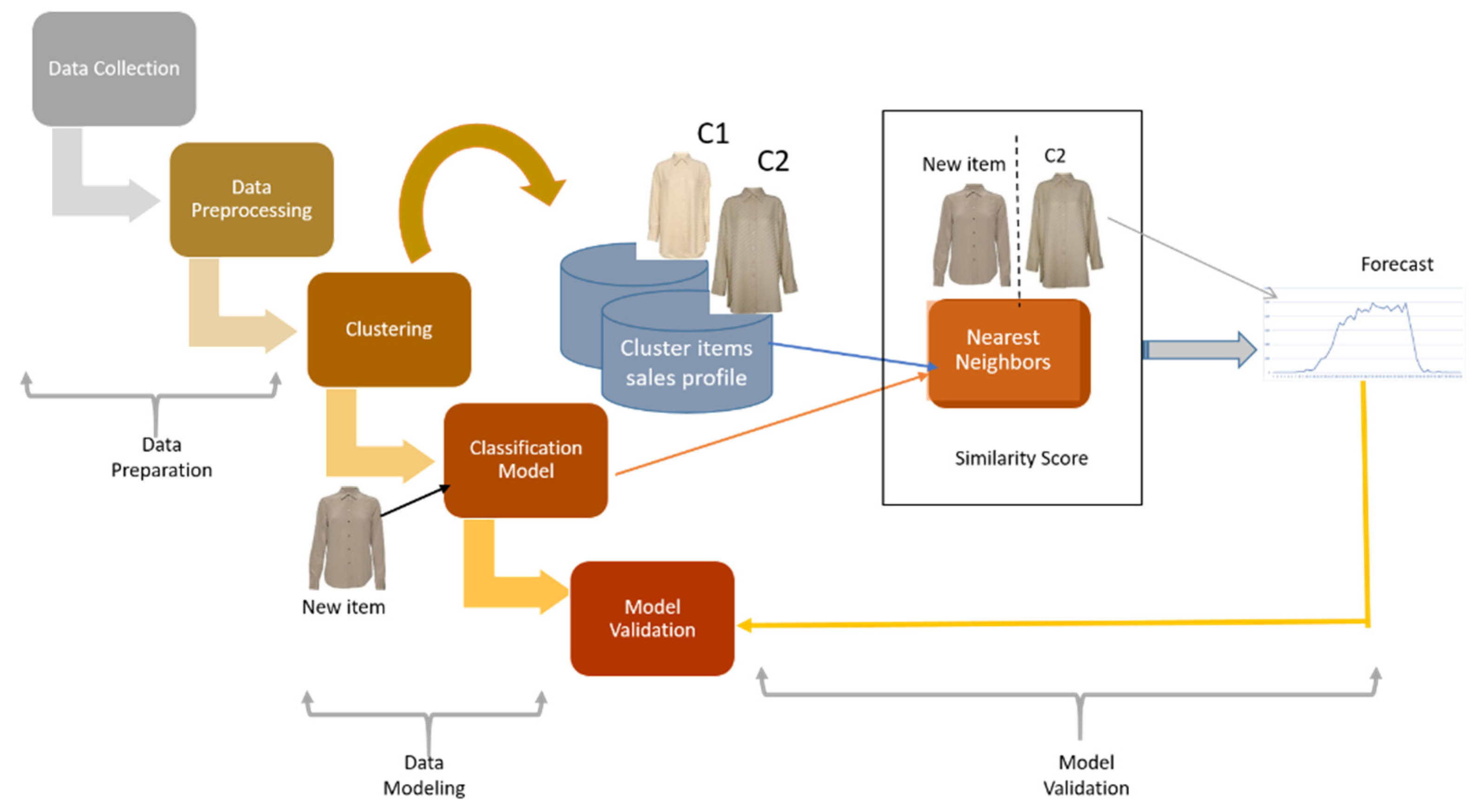
3.1. Experimental Design

This section presents the schema of all steps involved to carry out this experiment. The complete research workflow of sales forecasting is shown in Figure 1, which is broadly divided into three phases:
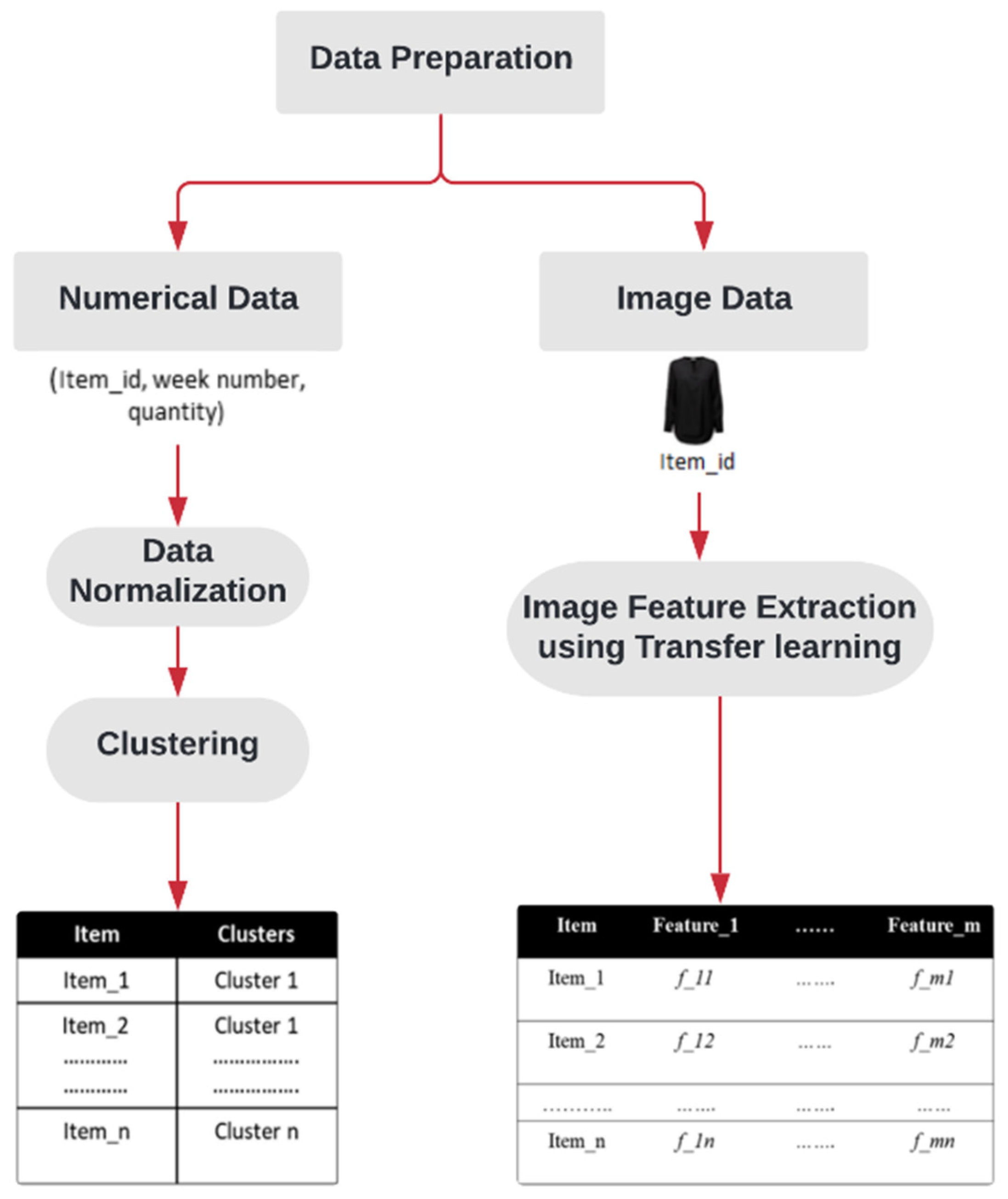
  • Data Preparation: This includes data collection and data pre-processing essential for data modelling.
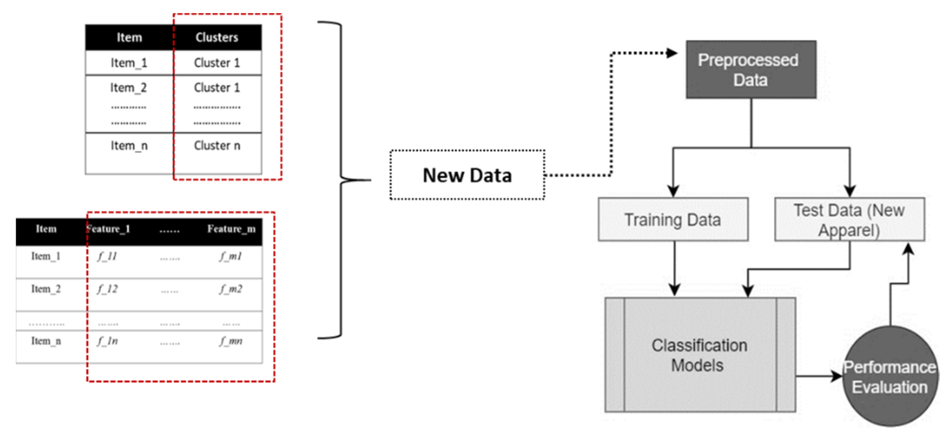
  • Data Modelling: In this step, pre-processed data are used for building the sales forecast model by using a machine learning algorithm.
  • Model Validation: In this step, the performance of the machine-learning model and forecast model is assessed.
All these phases are discussed in detail in the subsequent sections.

3.2. Machine Learning Algorithm

This section discusses the Machine learning methods and their evaluation metrics used for building the forecast model. This includes both supervised and unsupervised learning as explained in the following sections.

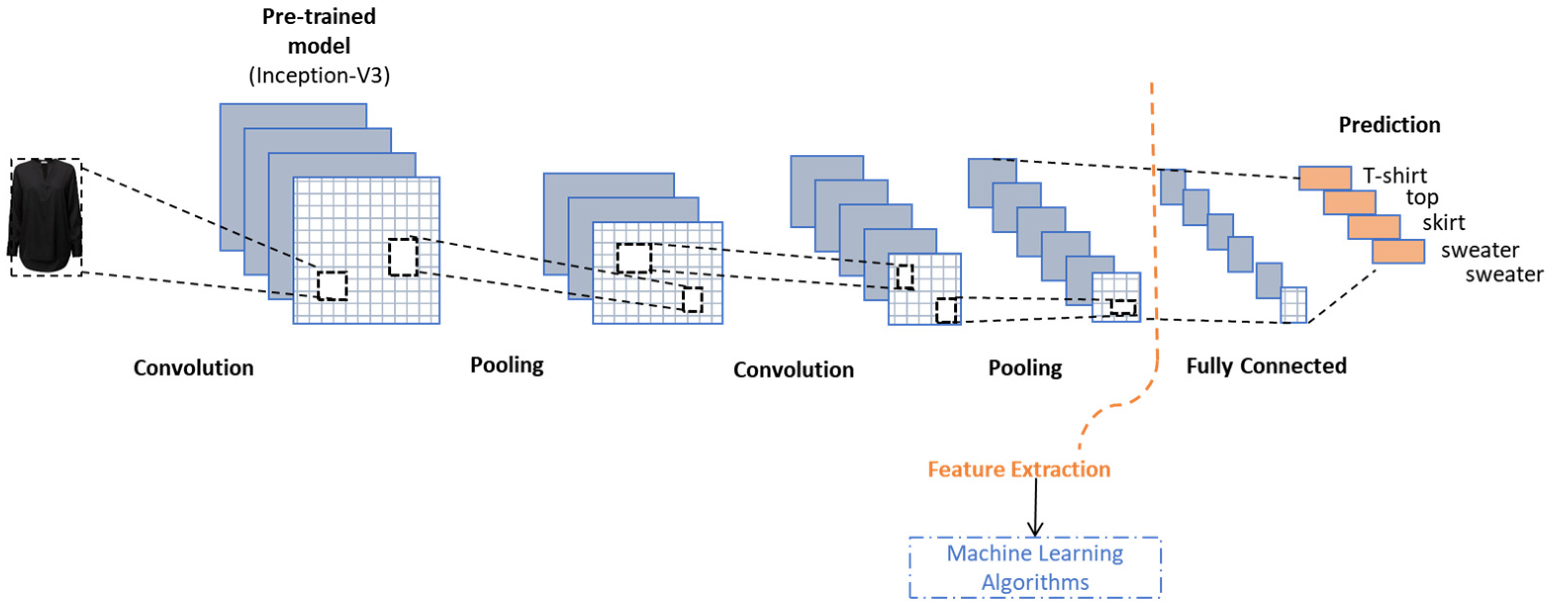
3.2.1. Deep Learning

In this study, deep learning is used for extracting product image features using CNN. The extracting feature is the dimensionality reduction of an image that signifies an image’s portions as a feature vector, as illustrated in Figure 2. Image features were extracted using a pre-trained deep learning inception v3 model [33]. This model has been chosen as it is trained on more than 1000 objects, which include fashion clothes and product images. The inception V3 model has outperformed the previous image recognition deep learning models ([33]).

3.2.2. Clustering

Clustering is an unsupervised learning method, and the main task of this algorithm is to group similar items using distance metrics. The input data are unlabelled, and the created cluster could be used as a label for another machine learning task. There are different clustering algorithms, such as K-means, hierarchal, and probabilistic clustering [23]. A classical K-means clustering is used for clustering the sales profile due to its easy application. The choice of optimum k was decided by the silhouette score [34]. It is calculated for each sample, and it is given by Equation (1), where A is the average distance to the nearby cluster and B is the mean intra-cluster distance. The value lies between 1 to −1; a value close to 1 indicates that the item is allocated to the correct cluster, whereas −1 indicates the assignment to the wrong cluster.
S i l h o u e t t e   C o e f f i c i e n t = A B   m a x A , B  

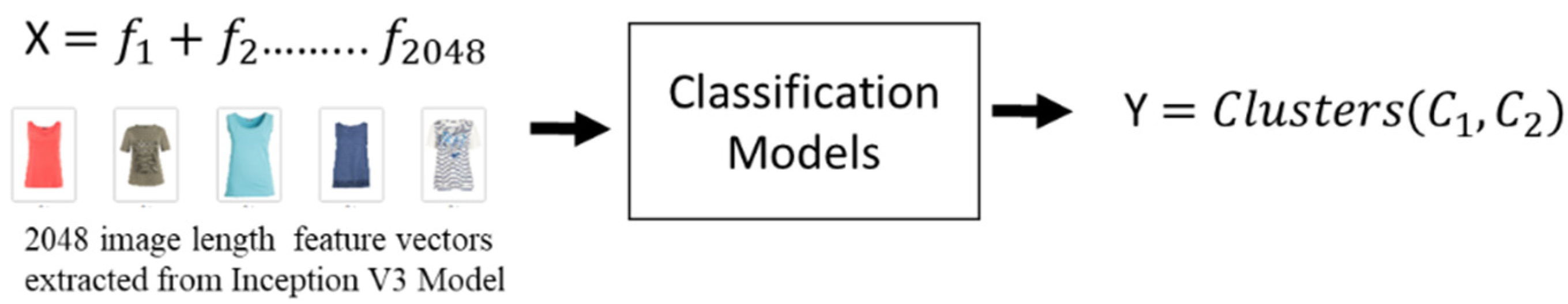
3.2.3. Classification

Classification is a supervised learning machine learning task where the model has input variables (X), and it maps the function to the output variable or target (Y). A simple classification model is represented in Equation (2). A problem can be considered a classification problem when the target variable is categorical.
Y = f (X)
For the classification model in this research study, the X variable represents the image features f 1 ,     f 2 , .. f n , and the Y variable represents the target variable, that is, cluster labels as illustrated in Figure 3.
Classification models, namely, Support Vector Machines (SVM), Random Forest (RF), Neural Network (NN), and Naïve Bayes (NB) [26,35,36] are applied in this research study. These classification algorithms are selected for comparatively analysing their performance in terms of the degree of their accuracy of classification. Moreover, the aim is also to identify the best-performing classification algorithm among the ones that are applied for the classification task.

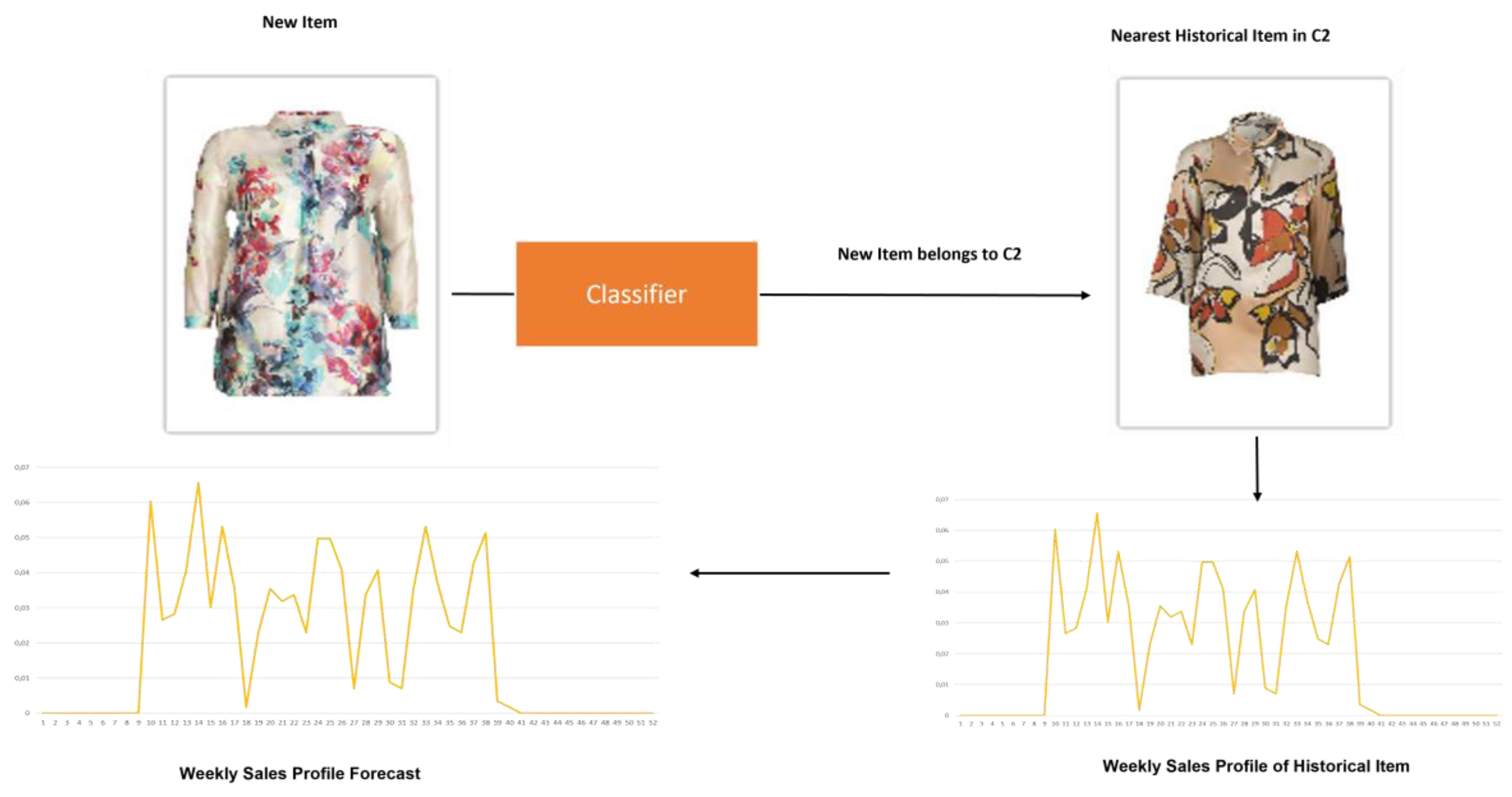
3.2.4. K Nearest Neighbour (k-NN)

This is a supervised algorithm that finds similar items that exist in the closest proximity based on the feature similarity. Feature similarities are calculated using Euclidian, Manhattan, and Cosine distance functions [36]. The use of k-NN is for finding the most similar image from the cluster database to the new items.

3.2.5. Evaluation Metrics

  • Classification:
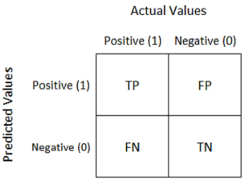
    • Classification accuracy (CA) is the proportion of correctly classified instances.
      C l a s s i f i c a t i o n   A c c u r a c y = T P + T N T P + T N + F P + F N  
      where,
      TP = True Positives, TN = True Negatives, FP = False Positives, and FN = False Negatives.
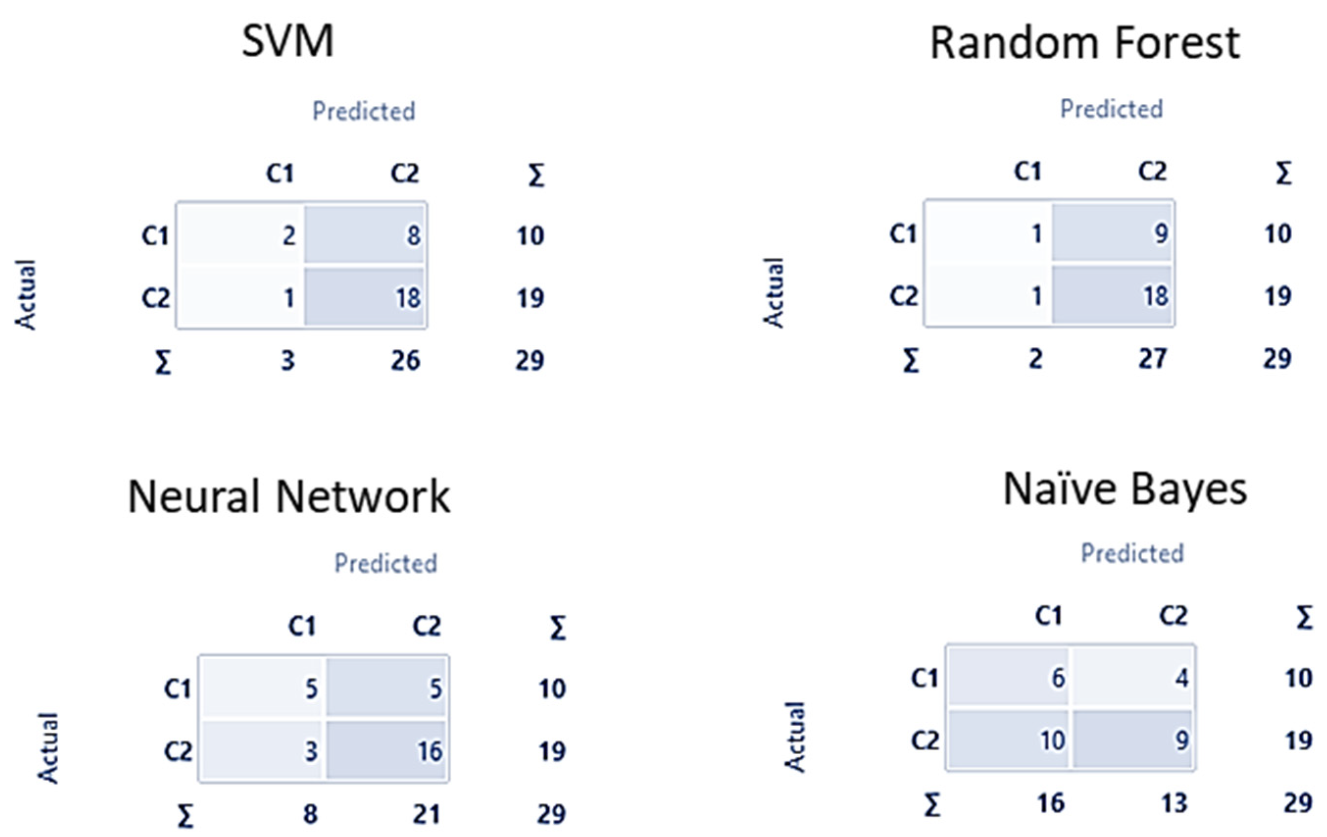
    • Confusion Matrix: It is used to represent the output of a classification model in a matrix format, where the rows represent the number of instances with a certain predicted label and the columns represent the number of instances with a certain correct label. A sample confusion matrix is shown in Figure 4.
    • Precision: It measures the proportion of positively classified instances that are actually positive.
      P r e c i s i o n = T P T P + F P    
    • Recall: It measures the proportion of positive instances that are actually predicted as positive.
      R e c a l l = T P T P + F N
    • F1 score: It is the harmonic mean of precision and recall. It provides a balance between Precision and Recall.
      F 1 = 2 × P r e c i s i o n × R e c a l l P r e c i s i o n + R e c a l l
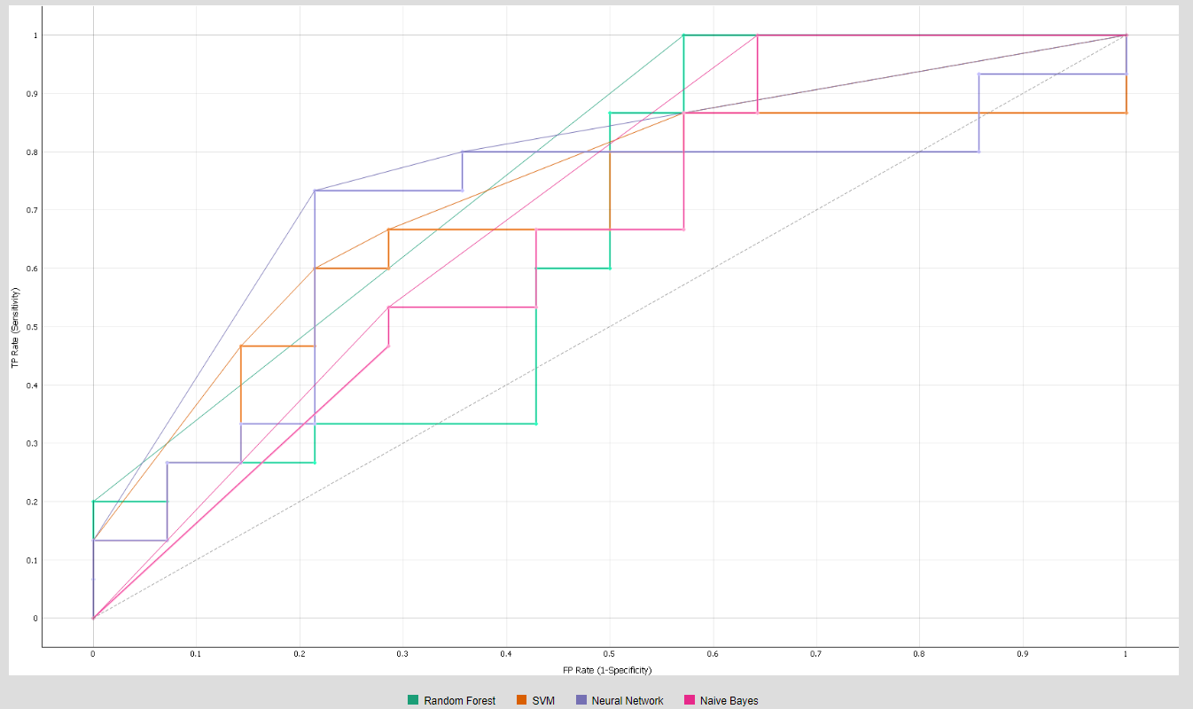
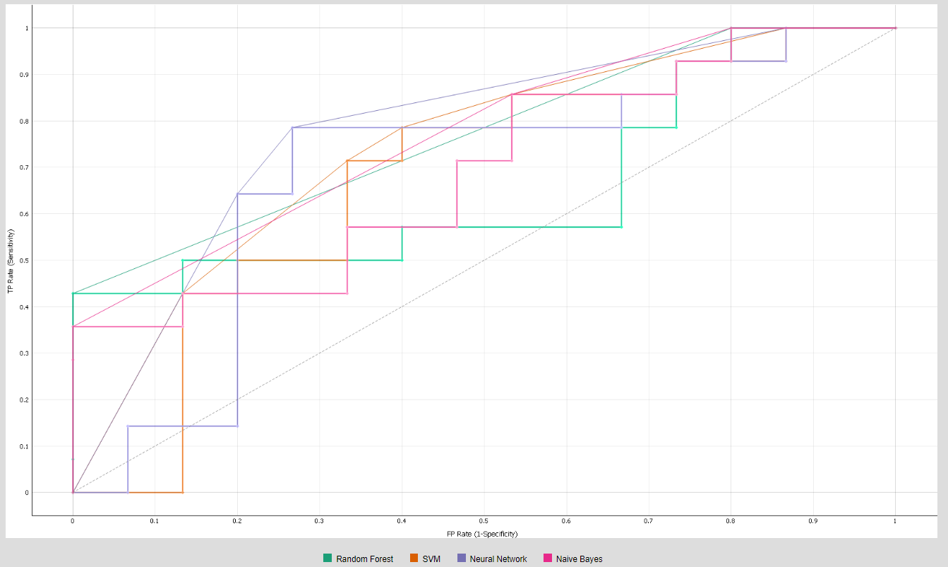
    • ROC curve: ROC curve is the measure for evaluating the quality of the classifier by plotting FPR along the X axis and the TPR along the Y axis [36].
    • AUC (Area Under the Curve): It measures the aggregated area under the ROC curve, and it comparatively evaluates the performances of different classification models. AUC threshold values range from (0, 0) to (1, 1), as represented in Figure 5. The value of AUC ranges from 0 to 1. The higher the value, the better the classification performance of the model.
  • Forecasting:
    • MAE (Mean Absolute Error) is the metric used for evaluating the forecast model performance.
      M A E = 1 n i = 1 n y i y ^ i  
      where, A t =   a c t u a l   s a l e s   a t   t i m e   t ,   F t = f o r e c a s t e d   s a l e s   a t   t i m e   t .
    • RMSE (root mean square error): It is the square root of MSE. It has the same unit as the target variable. MSE (Mean Squared Error) is a commonly used metric that measures the average squared difference between the target variable’s predicted value and its actual value
      R M S E = i = 1 i = n 1 n y i y ^ i 2  

3.3. Data Preparation

This section explains the steps involved in the preparation of data for the modelling.
This includes pre-processing product sales data, which has numerical and image data
attributes.
The data used in this study were collected from a European fashion retail company for a span of two years (2015, 2016), which consists of sales information of 290 items. The data attributes of these items are explained in Table 1. These data are characterised by numerical features and images (which are in pixels). It is vital to convert these images into vector form for mathematical modelling.
To accomplish data pre-processing, data normalisation was performed, which was essential to transform the data into a structured form that can be used for modelling. Hence, data pre-processing was carried out in two steps. First, a new feature was created using historical sales information of the product and secondly, image features were extracted using Inception V3, explained in Section 3.2, using image data, and the steps are illustrated in Figure 6.

3.3.1. Numerical Data

Numerical data have attributes Item no., Time and Quantity sold in Table 1. Quantity was aggregated weekly per item to create a new feature termed Sales Profile, and the step was repeated for each item using Equation (4), and a sample of the profile of an item is shown in Figure 7.
S a l e s   p r o f i l e   o f   a n   i t e m   I i = Q u a n t a t i t y   o f   i t e m   I i   s o l d   i n   a   w e e k   x T o t a l   Q u a n t i t y   o f   i t e m   I i   s o l d   i n   a   y e a r   52   w e e k s

3.3.2. Image Data

Image features were extracted using a pre-trained deep learning CNN inception V3 model, as explained in Section 3.2. Input images have a dimension of 360 × 540 × 3 at the pixel level. A feature vector of 2048 length was obtained using the CNN model, representing the feature of an image.

3.4. Modelling

This section explains the methodology used for modelling the sales data.

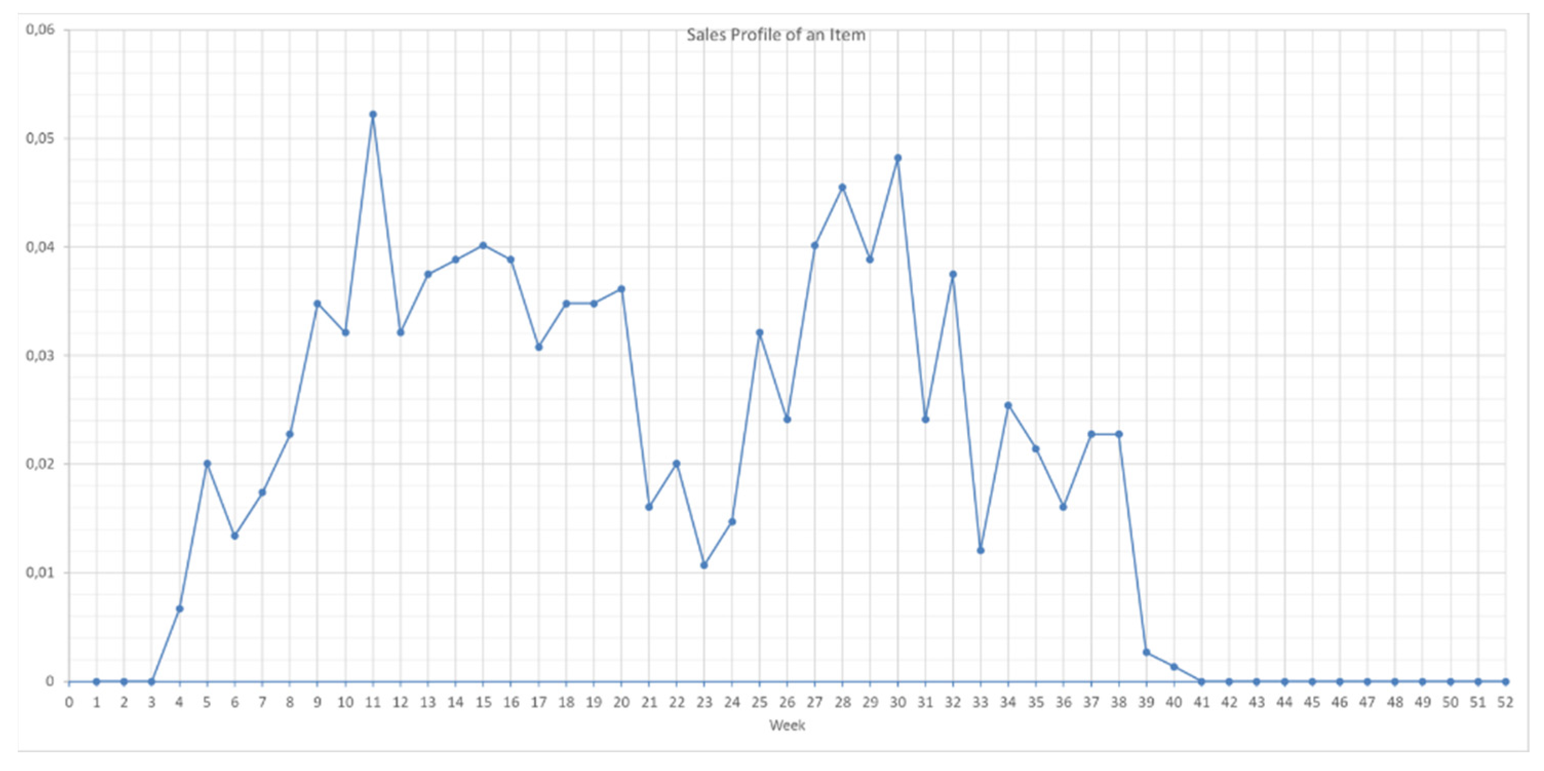
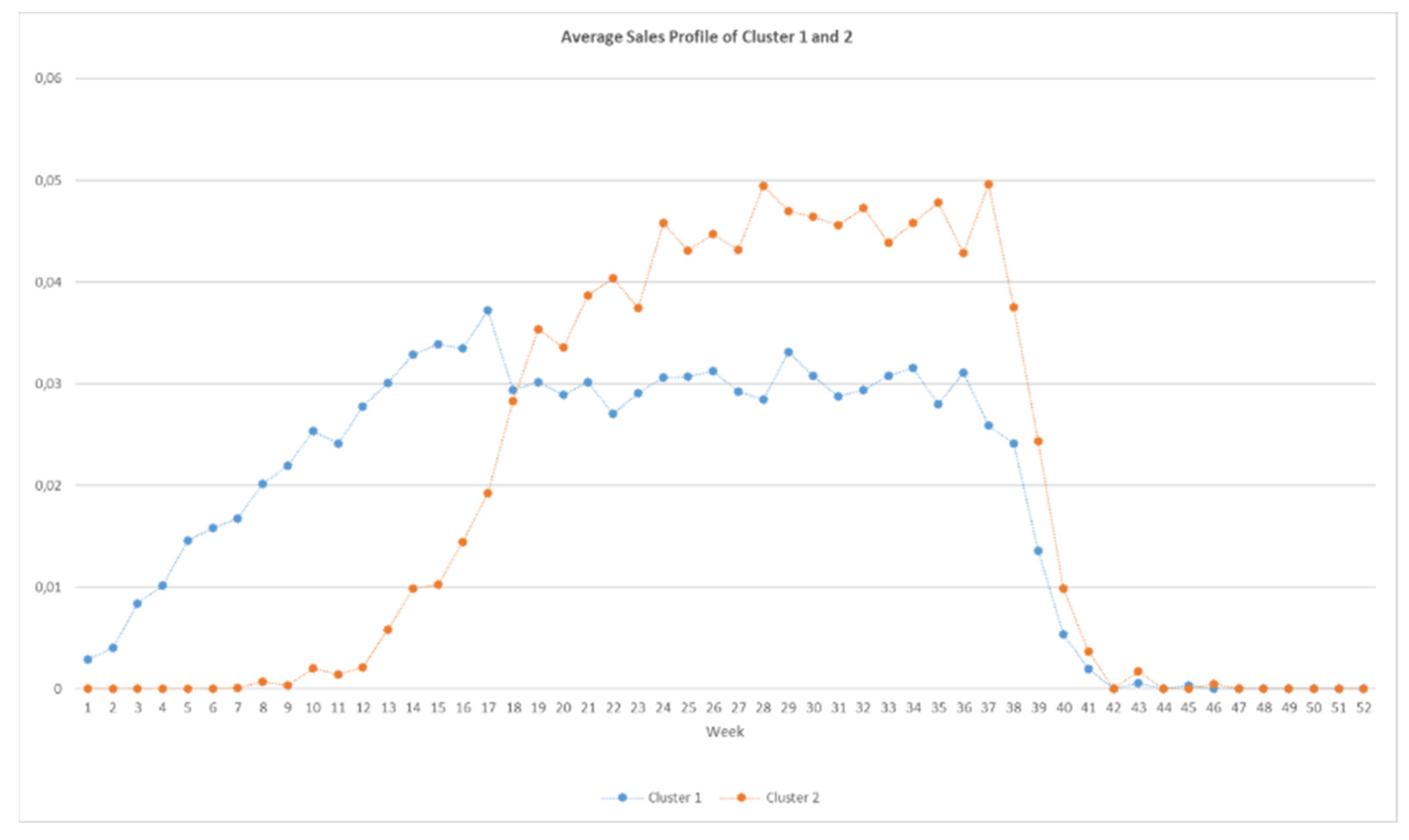
3.4.1. Clustering Sales Profile

Clustering was performed on the sales profile produced in Section 3.3. As a result, we computed Silhouette scores for each number of clusters to determine the optimum number of clusters in a dataset. The highest Silhouette score from Table 2, that is, 0,994, corresponded with the two clusters; therefore we chose two clusters of products’ sales profiles while performing k-means clustering. The average sales profile of two clusters C1 and C2 is shown in Figure 8. It can be observed that both the clusters exhibit varying average sales profiles. The average sale for C1 is from week 10 to week 43, and for C2, from week 1 to week 45. The obtained clusters are used as labels for the classification task discussed in the next section.

3.4.2. Cluster Classification Model

The pre-processed image data from Section 3.3.2 were labelled with clusters C1 and C2 as a target. These labelled data were used for training the classifier with image features as input and cluster labels as output. For this, data were divided into training and test data in the proportion of 90:10, as shown in Figure 9. As a result, training was done on 261 items, and the model was evaluated on 29 test items. Machine learning models SVM, RF, Naïve Bayes, and NN were used with their default training parameters for training the classifiers.

4. Experimental Results

This section presents the results of the cluster classification models discussed in Section 3.4. Section 4.1 summarises the comparative results of four classification models used to train the classifier. Further, Section 4.2 evaluates the forecast performance of test items with their actual sales.

4.1. Classification Model Performance

Classification models are used to train the classifier in Section 3.4, namely SVM, RF, NN, and NB. Applied classification models are evaluated on the test data, which contain 21 items using the metrics explained in Section 3.2. Results are shown in Table 3, which depicts that the classification model’s performance, Neural network (NN), has outperformed the other three models with the classification accuracy of 72.4% and AUC of 71.6%. However, the performance of the SVM and Random Forest are more than 65%, which is acceptable. While as, Naïve Bayes exhibited the most inferior performance overall. Therefore, we find that NN showed the best classification performance.
A confusion matrix was created for all four classification models, as shown in Figure 10, for examining the corrected classified items with the actual data. The test dataset consists of 29 items, of which 10 items go to C1, and 19 items go to C2. Items in C1 were poorly classified by SVM and RF, whereas NN and NB correctly classified 50%. Items in C2 were poorly classified by NB, while approximately 80% were classified correctly by SVM, RF, and NN. Further, ROC curves, as shown in Figure 11 and Figure 12, for each target class label, that is, C1 and C2, were plotted for all models to demonstrate the classification models’ results. It could be observed that NN has a better curve for both the clusters. Overall, NN shows a better prediction for both the clusters. Hence, based on the results, the NN model is the best model for this classification task, and the results of the test items in both the clusters will be assessed for forecast performance evaluation.

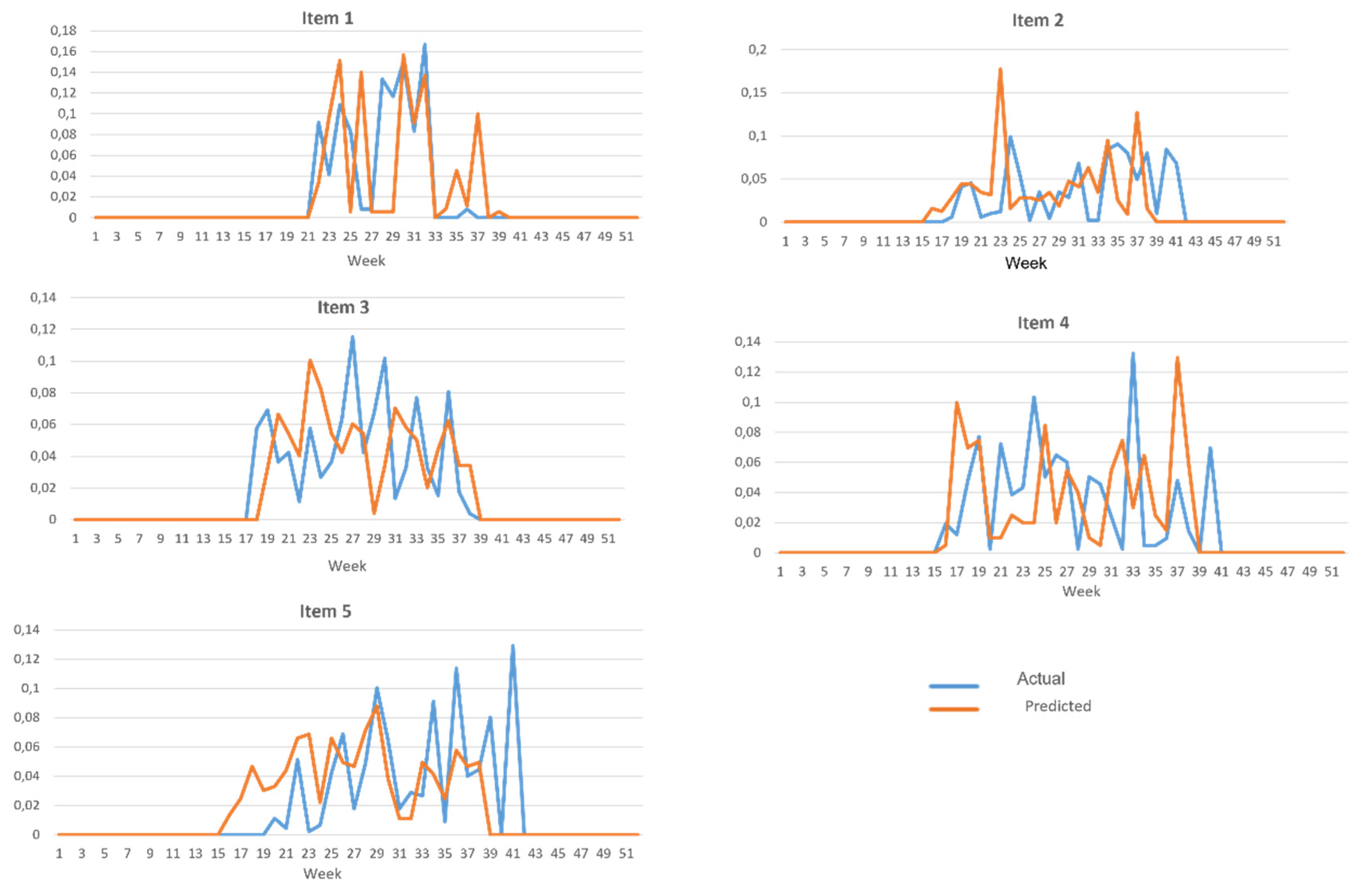
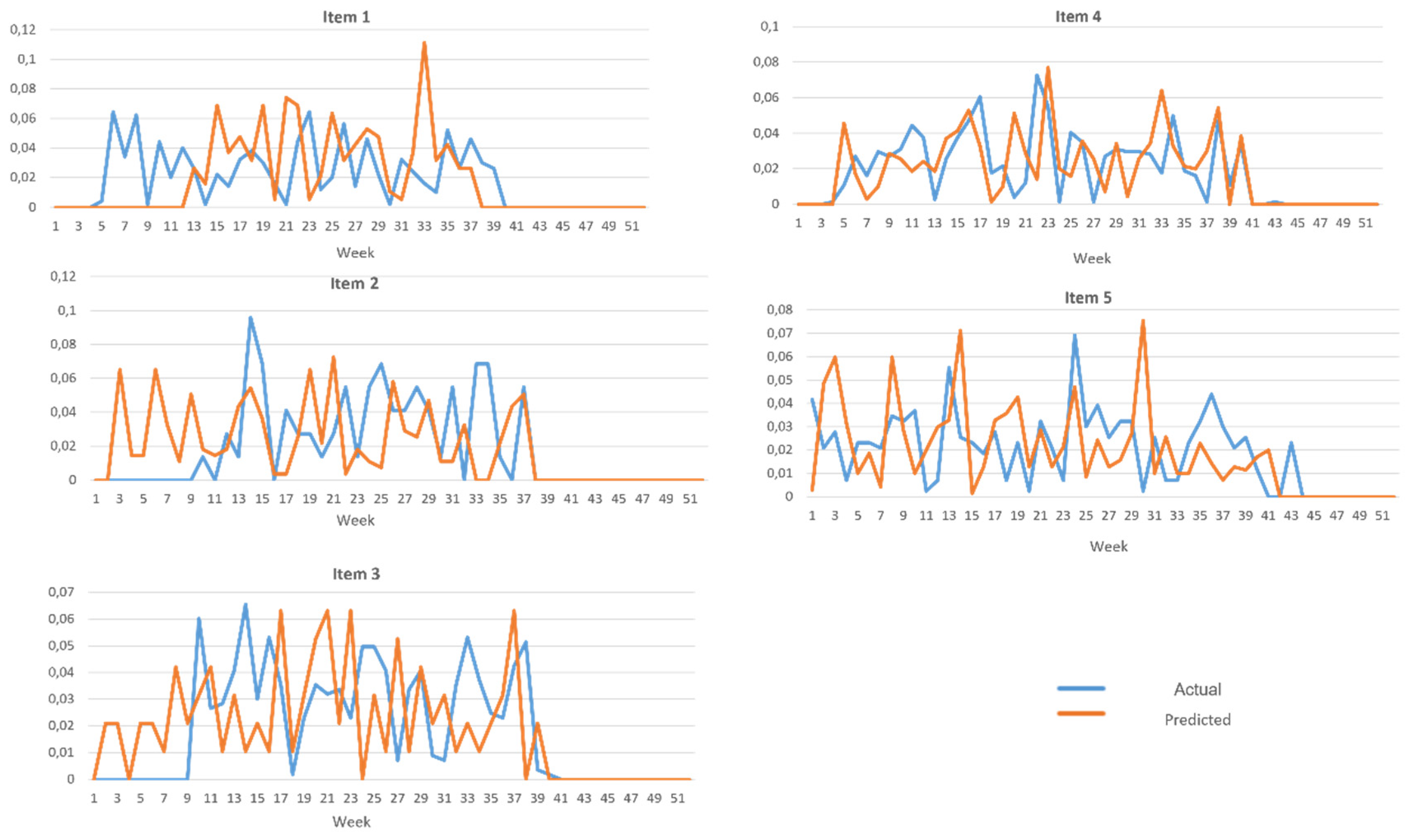
4.2. Forecast Performance Evaluation

The cluster classification model developed in Section 3.4 was trained to classify the new product based on their image and assign the cluster group. Hence, we have two cluster databases, namely C1 and C2. Once a new item is assigned to a cluster, it is then matched with other images in the same cluster using Cosine distance similarity. The identified closest image using the k-NN is then used to predict the sales profile of a new item. Complete system integration is presented in Figure 1, and the sample prediction result is presented in Figure 13.
Considering correctly classified items of the NN model, we have five items in C1 and 16 in C2. These items were used for validating the weekly forecast predicted by the model with the actual sales profile of the data. The used metrics were RMSE and MAE, as shown in Table 3. The average RMSE for C1 is 0,0328, and MAE is 0,0168, and for C2, RMSE is 0,0248 and MAE is 0,01631. Results in Table 4 show that the average RMSE and MAE for C2 are better than C1. The reason for this could be the number of training instances, which was more for C2 than C1.
The predicted sales profiles of correctly classified five items from both clusters are illustrated in Figure 14 and Figure 15. The results clearly show that the model prediction was reasonably accurate as it is closer to the value of actual sales.
In the illustrations of five items of C1, as shown in Figure 14, we can see that items 1, 2, 3, and 5 are following the trend of the actual sales with some fluctuations from week 29 to week 37. The sales for the items were predicted before the actual sales, that is, from week 16, and it shows no sales after week 39, so two weeks lag was seen in this case.
Similarly, for items in C2, as shown in Figure 15, especially for item 1, there was no prediction for the week from 4 to 12, after that trend has followed the actual sales with some fluctuations. Whereas for some items, such as items 2 and 3, the prediction was made ahead, and for items 4 and 5, the trend was followed with some variations from the actual sales.
The forecast (prediction) of weekly sales given by the model is close to the actual sales, and results using RMSE and MAE have small errors, as shown in Table 4.

5. Discussion

This paper aimed at proposing a novel sales forecast approach for fashion products using machine learning clustering and classification techniques. Real fashion retail data have been utilised to train the clustering and classification models, and their performances are comparatively measured based on evaluation metrics described in Section 3.2.5. These metrics were also used to interpret the results of each applied machine learning model and based on which the best performing classification model is identified.
Table 3 contains the performance values of the classification models with respect to the evaluation metrics such as AUC, CA, F1 Score, Precision, and Recall. Of all the classification models, it is found that NN showed the best performance given its highest CA value, that is, 0,724. In terms of performance based on AUC, both Figure 11 and Figure 12 illustrate that the ROC curve of NN is close to value 1 for both the classes, that is, C1 and C2. As the next step, the closest match of a new fashion item is found in the Cluster by using the k-NN model. The sales profile of a closely matching fashion item is the forecast of a new item’s sales profile. The accuracy of this forecast is computed using metrics such as MAE and RMSE, which have been explained in Section 3.2.5. Table 4 contains the RMSE and MAE values for each correctly classified item in both the clusters, that is, C1 and C2. The performance metrics of the sales forecast of the new items belonging to C2 show a higher score than for C1. Overall, the model results are promising and demonstrate that the proposed sales forecast model based on clustering and classification models could be effectively used for short-term prediction (weekly sales) of a new fashion clothing item and could enable the fashion retail industry to manage their inventory replenishment effectively based on demonstrated forecast results.

6. Conclusions

A novel forecasting model was developed to predict the sales profile for a new fashion apparel product using machine learning and deep learning algorithms. This study was conducted on real sales data, which contain historical information on sales with product images. Taking into account forecast model performance, we conclude that this model could be valuable for the fashion clothing industry for managing various supply chain planning tasks. This research demonstrates that images, along with the historical information of an item, can be used for forecasting the sales of a new item in the fashion retailing industry. As this forecasting approach can be sensitive to product images, it is crucial to consider the databases to train it with more images and enhance the classification accuracy. Apart from this, the model performance could be improved by training the image data by using CNN independently instead of transfer learning.
In future work, we can enhance the image database for improving model accuracy. Also, a detailed comparative study could be performed by comparing the model performance with classical forecasting models.

Author Contributions

The study was designed and completed with the support of Y.C., C.G. was responsible for data collection, experimental analysis, and structuring of the manuscript. Y.C. contributed to interpreting the findings and refining the script. All authors have read and agreed to the published version of the manuscript.

Funding

This research work is conducted under the framework of the SMDTex project (2017–2021) funded by the European Commission.

Institutional Review Board Statement

Not applicable.

Informed Consent Statement

Not applicable.

Data Availability Statement

Not applicable.

Acknowledgments

We are grateful to the Evo Pricing company for providing the data for this research work.

Conflicts of Interest

The author declares no conflict of interest.

References

  1. Giri, C.; Thomassey, S.; Zeng, X. Customer Analytics in Fashion Retail Industry. In Functional Textiles and Clothing; Springer: Singapore, 2019; pp. 349–361. [Google Scholar]
  2. Minner, S.; Kiesmller, G.P. Dynamic product acquisition in closed loop supply chains. Int. J. Prod. Res. 2012, 50, 2836–2851. [Google Scholar] [CrossRef] [Green Version]
  3. Thomassey, S. Economics and undefined 2010, Sales forecasts in clothing industry: The key success factor of the supply chain management. Int. J. Prod. Econ. 2010, 128, 470–483. [Google Scholar] [CrossRef]
  4. Giri, C.; Thomassey, S.; Zeng, X. Exploitation of Social Network Data for forecasting Garment Sales. Int. J. Comput. Intell. Syst. 2019, 12, 1423. [Google Scholar] [CrossRef] [Green Version]
  5. Giri, C.; Thomassey, S.; Balkow, J.; Zeng, X. Forecasting New Apparel Sales Using Deep Learning and Nonlinear Neural Network Regression. In Proceedings of the 2019 International Conference on Engineering, Science, and Industrial Applications, Tokyo, Japan, 22–24 August 2019; ICESI 2019. [Google Scholar]
  6. Christopher, M.; Lee, H. Mitigating supply chain risk through improved confidence. Int. J. Phys. Distrib. Logist. Manag. 2004, 34, 388–396. [Google Scholar] [CrossRef] [Green Version]
  7. Christopher, M.; Towill, D. An integrated model for the design of agile supply chains. Int. J. Phys. Distrib. Logist. Manag. 2001, 31, 235–246. [Google Scholar] [CrossRef] [Green Version]
  8. Battista, C.; Schiraldi, M.M. The Logistic Maturity Model: Application to a fashion firm. Int. J. Eng. Bus. Manag. 2013, 5, 1–11. [Google Scholar] [CrossRef] [Green Version]
  9. Nayak, R.; Padhye, R. Artificial intelligence and its application in the apparel industry. In Automation in Garment Manufacturing; Elsevier Inc.: Amsterdam, The Netherlands, 2018; pp. 109–138. [Google Scholar] [CrossRef]
  10. Giri, C.; Jain, S.; Zeng, X.; Bruniaux, P. A Detailed Review of Artificial Intelligence Applied in the Fashion and Apparel Industry. IEEE Access 2019, 7, 95376–95396. [Google Scholar] [CrossRef]
  11. Papalexopoulos, A.D.; Hesterberg, T.C. A regression-based approach to short-term system load forecasting. In Proceedings of the Conference Papers Power Industry Computer Application Conference, Roanoke, VA, USA, 21 May 1999; pp. 414–423. [Google Scholar]
  12. Healy, M.J.R.; Brown, R.G. Smoothing, Forecasting and Prediction of Discrete Time Series. J. R. Stat. Soc. Ser. A 1964, 127, 292. [Google Scholar] [CrossRef]
  13. de Gooijer, J.G.; Hyndman, R.J. 25 Years of Time Series Forecasting; Elsevier: Amsterdam, The Netherlands, 2006. [Google Scholar] [CrossRef] [Green Version]
  14. Box, G.E.P.; Jenkins, G.M. Time Series Analysis: Forecasting and Control; Prentice Hall: Hoboken, NJ, USA, 1976. [Google Scholar]
  15. Hui, P.C.L.; Choi, T.-M. Using artificial neural networks to improve decision making in apparel supply chain systems. In Information Systems for the Fashion and Apparel Industry; Elsevier: Amsterdam, The Netherlands, 2016; pp. 97–107. [Google Scholar]
  16. Makridakis, S.; Wheelwright, S.; Hyndman, R. Forecasting Methods and Applications; John Wiley & Sons: New York, NY, USA, 1998. [Google Scholar]
  17. Wong, W.K.; Guo, Z.X. A Hybrid Intelligent Model for Medium-Term Sales Forecasting in Fashion Retail Supply Chains Using Extreme Learning Machine and Harmony Search Algorithm; Elsevier: Amsterdam, The Netherlands, 2010. [Google Scholar]
  18. Chu, W.C.; Zhang, P.G. A comparative study of linear and nonlinear models for aggregate retail sales forecasting. Int. J. Prod. Econ. 2003, 86, 217–231. [Google Scholar] [CrossRef]
  19. Thiesing, F.M.; Vornberger, O. Forecasting sales using neural networks. In International Conference on Computational Intelligence; Springer: Berlin/Heidelberg, Germany, 1997; Volume 1226, pp. 321–328. [Google Scholar]
  20. Alon, I.; Qi, M.; Sadowski, R.J. Forecasting aggregate retail sales: A comparison of artificial neural networks and traditional methods. J. Retail. Consum. Serv. 2001, 8, 147–156. [Google Scholar] [CrossRef]
  21. Ansuj, A.P.; Camargo, M.; Radharamanan, R.; Petry, D. Sales forecasting using time series and neural networks. Comput. Ind. Eng. 1996, 31, 421–424. [Google Scholar] [CrossRef]
  22. Chang, P.-C.; Wang, Y.; Tsai, C. Evolving neural network for printed circuit board sales forecasting. Expert Syst. Appl. 2005, 29, 83–92. [Google Scholar] [CrossRef]
  23. Russell, S.J.; Norvig, P.; Davis, E. Artificial Intelligence: A Modern Approach; Pearson Education, Inc.: New York, NY, USA, 2010. [Google Scholar]
  24. Laney, D. 3D Data Management: Controlling Data Volume, Velocity, and Variety. META Group Res. Note 2001, 6, 1. [Google Scholar]
  25. Zadeh, L.A. Fuzzy sets. Inf. Control 1965, 8, 38–353. [Google Scholar] [CrossRef] [Green Version]
  26. Tan, P.-N.; Steinbach, M.; Kumar, V. Introduction to Data Mining; Pearson Addison Wesley: Boston, MA, USA, 2005. [Google Scholar]
  27. LeCun, Y.; Bengio, Y.; Hinton, G. Deep learning. Nature 2015, 521, 436–446. [Google Scholar] [CrossRef] [PubMed]
  28. Jiang, S.; Chin, K.-S.; Wang, L.; Qu, G.; Tsui, K.L. Modified genetic algorithm-based feature selection combined with pre-trained deep neural network for demand forecasting in outpatient department. Expert Syst. Appl. 2017, 82, 216–230. [Google Scholar] [CrossRef]
  29. Xu, S.; Chan, H.K.; Zhang, T. Forecasting the demand of the aviation industry using hybrid time series SARIMA-SVR approach. Transp. Res. Part E Logist. Transp. Rev. 2019, 122, 169–180. [Google Scholar] [CrossRef]
  30. Qiu, X.; Ren, Y.; Suganthan, P.N.; Amaratunga, G.A.J. Empirical Mode Decomposition based ensemble deep learning for load demand time series forecasting. Appl. Soft Comput. 2017, 54, 246–255. [Google Scholar] [CrossRef]
  31. Alibabaei, K.; Gaspar, P.D.; Lima, T.M.; Campos, R.M.; Girão, I.; Monteiro, J.; Lopes, C.M. A Review of the Challenges of Using Deep Learning Algorithms to Support Decision-Making in Agricultural Activities. Remote Sens. 2022, 14, 638. [Google Scholar] [CrossRef]
  32. Thomassey, S.; Happiette, M. A neural clustering and classification system for sales forecasting of new apparel items. Appl. Soft Comput. 2007, 7, 1177–1187. [Google Scholar] [CrossRef]
  33. Szegedy, C.; Vanhoucke, V.; Ioffe, S.; Shlens, J.; Wojna, Z. Rethinking the Inception Architecture for Computer Vision. In Proceedings of the 2016 IEEE Conference on Computer Vision and Pattern Recognition (CVPR), Las Vegas, NV, USA, 27–30 June 2016; pp. 2818–2826. [Google Scholar]
  34. Aranganayagi, S.; Thangavel, K. Clustering categorical data using silhouette coefficient as a relocating measure. In Proceedings of the International Conference on Computational Intelligence and Multimedia Applications (ICCIMA 2007), Sivakasi, Tamil Nadu, 13–15 December 2007. [Google Scholar]
  35. Manning, C.D.; Raghavan, P.; Schutze, H. Introduction to Information Retrieval; Cambridge University Press: Cambridge, UK, 2008. [Google Scholar]
  36. Bishop, C.M.; Nasrabadi, N.M. Pattern Recognition and Machine Learning; Springer: New York, NY, USA, 2006. [Google Scholar]
Figure 1. Experimental design.
Forecasting 04 00031 g001
Figure 2. Product image feature extraction.
Forecasting 04 00031 g002
Figure 3. Classification model representation.
Forecasting 04 00031 g003
Figure 4. A confusion matrix.
Forecasting 04 00031 g004
Figure 5. A sample ROC curve.
Forecasting 04 00031 g005
Figure 6. Data pre-processing.
Forecasting 04 00031 g006
Figure 7. Sample sales profile of an item (In this research work, comma (,) is used as decimal separators for figure and result values).
Forecasting 04 00031 g007
Figure 8. Average sales profile of clusters.
Forecasting 04 00031 g008
Figure 9. Classification model.
Forecasting 04 00031 g009
Figure 10. Confusion matrix.
Forecasting 04 00031 g010
Figure 11. ROC curve of classification models for Cluster 1.
Forecasting 04 00031 g011
Figure 12. ROC curve of classification models for Cluster 2.
Forecasting 04 00031 g012
Figure 13. Sample sales profile forecast of Test item.
Forecasting 04 00031 g013
Figure 14. Sales profile of five items from C1 (predicted vs. actual).
Forecasting 04 00031 g014
Figure 15. Sales profile of five items from C2 (predicted vs. actual).
Forecasting 04 00031 g015
Table 1. Data attributes.
Data AttributesDescription
Item NoUnique id
Image360 × 540 × 3 pixels
Quantity SoldAmount of the items sold
Timeweeks
Table 2. Silhouette Scores.
KSilhouette Scores
20,994
30,600
40,435
50,227
60,210
70,236
80,111
90,131
100,120
Table 3. Results.
Table 3. Results.
ModelAUCCAF1PrecisionRecall
SVM0,6210,6900,6300,6830,689
RF0,5260,6550,5700,6090,655
NN0,7160,7240,7160,7140,724
NB0,6260,5170,5280,5830,517
Table 4. Forecast evaluation.
Correctly Classified ItemsRMSEMAE
Cluster 1 (C1)Item 10,03750,0156
Item 20,03830,0202
Item 30,02450,0138
Item 40,03450,0193
Item 50,02900,0153
Average0,03280,0169
Cluster 2(C2)Item 10,02910,0187
Item 20,02960,0195
Item 30,02290,0168
Item 40,01800,0117
Item 50,02050,0152
Item 60,02360,0168
Item 70,03030,0182
Item 80,02160,0141
Item 90,02320,0155
Item 100,03100,0204
Item 110,02290,0136
Item 120,02040,0131
Item 130,02010,0123
Item 140,03400,0201
Item 150,02830,0186
Item 160,02200,0134
Average0,02480,0163
Publisher’s Note: MDPI stays neutral with regard to jurisdictional claims in published maps and institutional affiliations.

