Evaluating State-of-the-Art, Forecasting Ensembles and Meta-Learning Strategies for Model Fusion

Abstract

The techniques of hybridisation and ensemble learning are popular model fusion techniques for improving the predictive power of forecasting methods. With limited research that instigates combining these two promising approaches, this paper focuses on the utility of the Exponential Smoothing-Recurrent Neural Network (ES-RNN) in the pool of base learners for different ensembles. We compare against some state-of-the-art ensembling techniques and arithmetic model averaging as a benchmark. We experiment with the M4 forecasting dataset of 100,000 time-series, and the results show that the Feature-Based FORecast Model Averaging (FFORMA), on average, is the best technique for late data fusion with the ES-RNN. However, considering the M4’s Daily subset of data, stacking was the only successful ensemble at dealing with the case where all base learner performances were similar. Our experimental results indicate that we attain state-of-the-art forecasting results compared to Neural Basis Expansion Analysis (N-BEATS) as a benchmark. We conclude that model averaging is a more robust ensembling technique than model selection and stacking strategies. Further, the results show that gradient boosting is superior for implementing ensemble learning strategies.

1. Introduction

Forecasting is the procedure of creating predictions based on past and current data. Subsequently, these predictions can be compared against what happens. For example, one might estimate future infections and then compare them against the actual outcomes. Forecasting might refer to specific formal statistical methods employing time-series, cross-sectional or longitudinal data, less traditional judgmental methods or the process of prediction and resolution itself [1].

Although challenging, forecasting time-series is an essential task to which substantial research effort has been applied. Makridakis et al. [2] emphasised two facts about the field: first, no one has prophetic powers to predict the future accurately, and second, all predictions are subject to uncertainty, especially within social contexts.

Forecasting has applications in many fields where estimates of future conditions are helpful. Depending on the area, accuracy varies significantly. If the factors that relate to the forecast are known and well understood and a significant amount of data can be used, the final value will likely be close to the estimates. If this is not the case or if the actual outcome is affected by the forecast, the dependability of the predictions can be significantly lower. Some forecasting applications include climate change, preventative maintenance, anomalies, stock returns, epidemics, economic trends and the development of conflict situations [3,4,5,6].

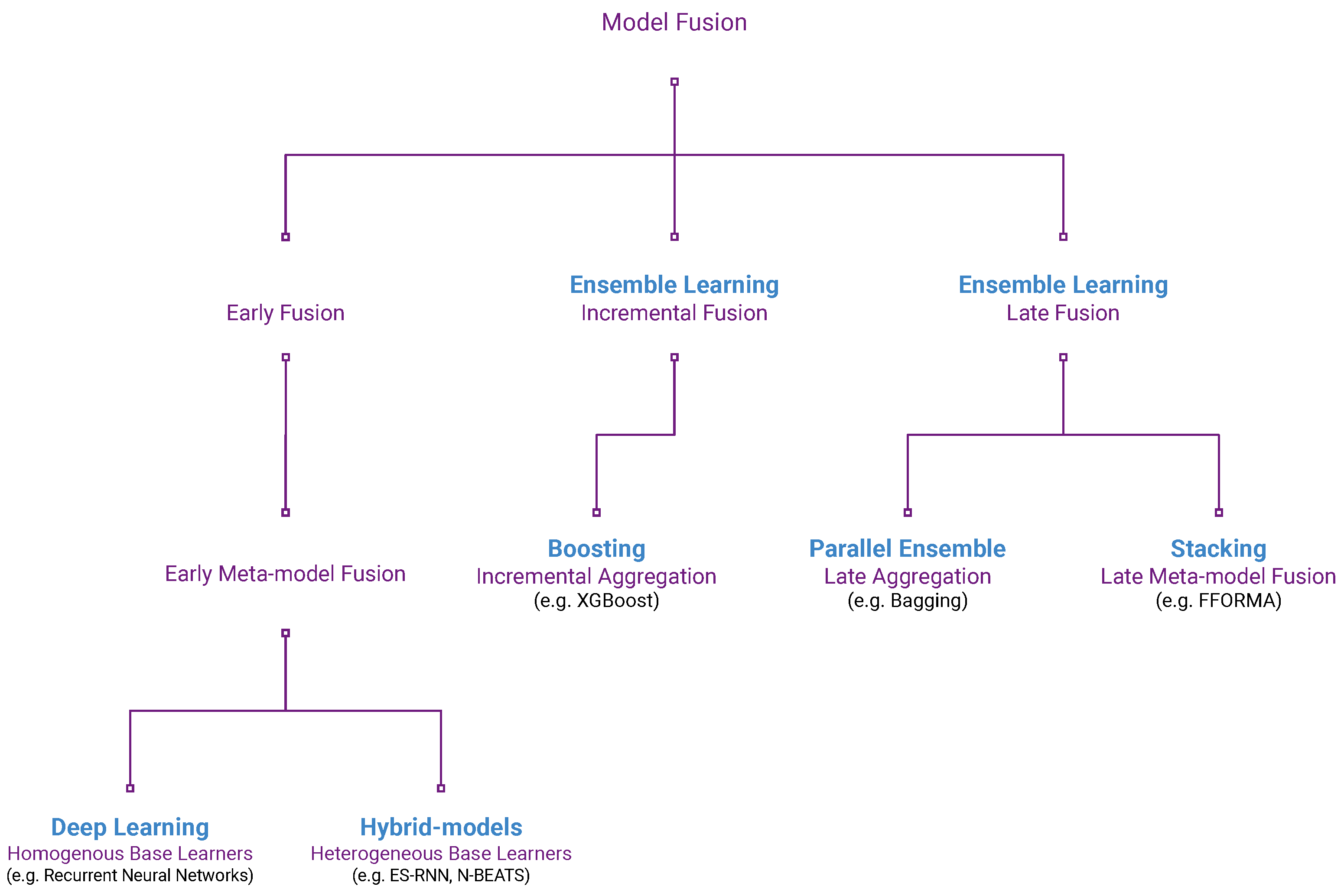
1.1. Model Fusion and Meta-Learning

In this section, we refine the concepts of meta-learning and model fusion and present a brief framework to better contextualise the later literature review as it relates to the presented forecasting techniques. First, we give a definition of model fusion as it relates to forecasting and how it differs from traditional data fusion. Next, we describe what meta-learning is within the context of model fusion for time-series forecasting.

Data fusion is the multimodal, multiresolution, multitemporal process of integrating data sources to produce more consistent, accurate and useful information than the sources individually. Traditional multimodal data fusion approaches are grouped into classes, based on the processing level at which the fusion occurs: early fusion or data-level fusion, late fusion or decision-level fusion and intermediate fusion, which combines late and early approaches [7].

Analogously, we define model fusion as integrating base learners to produce a lower bias and variance and a more robust, consistent and accurate model than that of the learners individually. These base learners can either be homogeneous from the same hypothesis class (e.g., decision trees in a random forest) or be heterogeneous from different hypothesis classes (e.g., a neural network with a support vector machine for classification). Drawing further from multimodal data fusion, which subcategorises based on the whether or not the fusion process is early or late, we present definitions for early model fusion, late model fusion and incremental model fusion. We define these terms as follows:

• Early model fusion integrates the base learners before training. The combined model is then trained as a single fused model.
• Late model fusion first trains the base learners individually. The now pretrained base learners are then integrated without further modification.
• Incremental model fusion performs model integration while training the base learners incrementally. Each combined base learner’s parameters remain fixed once trained.

An important aspect of model fusion is that of meta-learning. Meta-learning is typically classified into metric-based, model-based and optimisation-based meta-learning. Of interest in our discussion is model-based meta-learning. Model-based meta-learning uses meta-data/meta-features about the problem together with a meta-model to improve overall performance. For instance, stacked generalisation works by using linear regression to weight heterogeneous base learners [8]. We are now in a position to define the model integration process:

• Meta-model fusion uses model-based meta-learning to perform the model integration process.
• Aggregation fusion, or just aggregation, uses a simple aggregation scheme, such as weighted averaging, to perform the model integration process.

Combing the above discussion with the commonly used appellative for the classes of techniques allows us to arrive at the following incomplete taxonomy shown in Figure 1. In the following section, we review the relevant literature for forecasting model fusion in the context of the presented taxonomy.

1.2. Related Literature

Despite the diversity of the forecasting models, the no free lunch theorem holds that no single algorithm universally outperforms any other for all problems [11]. As a result, an essential question is raised about choosing the best algorithm for a specific time-series. These many techniques are underpinned by different principles to perform forecasting. However, numerous forecasting studies have shown that a fusion of models generally outperforms the individuals [12,13,14].

Arinze [8] first introduced meta-learning as a stacking technique to select one forecasting model among six others based on the learnt performance for six time-series meta-features (e.g., autocorrelation, trend and coefficients). Raftery et al. [15] pointed out that single model selection is open to issues of model uncertainty and proposed using Bayesian model averaging for stacking instead. Bayesian model averaging makes weighted average predictions as the posterior probability of each model being correct given the same dataset. Stacking can also learn the weights from the predictions of heterogeneous base learners using cross-validation instead of using posterior probabilities [16]. Clarke [16] reported cross-validation-based stacking as a more robust method than Bayesian model averaging for computations that involve sensitive changes over their variables.

Stacking methods’ performance might also be improved by utilising additional time-series statistics as meta-features in the learning process. Cawood and van Zyl [1], for example, proposed a feature-weighted stacking approach that improves the regression from base learner predictions by supplementing them with time-series statistics extracted from the input series. Recent work has established many valuable statistics for meta-learning, including, but not limited to, linearity, curvature, autocorrelation, stability and entropy [17,18,19].

Ribeiro and Coelho [9] studied contemporary ensemble methods in forecasting time-series within agribusiness. In their work, they compare approaches of bagging with Random Forests (RF), boosting with gradient boosting machines (XGBoost), and a stacked generalisation of machine learning models. Ribeiro and Coelhoa’s findings suggest that gradient boosting methods generally produce the lowest prediction errors. The top two submissions of the M4 forecasting competition both implement ensemble learning to produce state-of-the-art results.

The runner-up in the M4 Competition, FFORMA, implements stacking using extreme gradient boosting to learn the weightings for the base learners based on several meta-features extracted from the input time-series [19]. The weightings learned by the trained meta-model are then used to combine the model’s predictions as a feature-weighted average.

Hybrid approaches combine linear and nonlinear models since time-series are rarely pure linear or nonlinear in reality [10]. Hybrid forecasting models were first proposed by Zhang [10], who showed that the hybridisation of the ARIMA and Multilayer Perceptron (MLP) models yields improved accuracy since it takes advantage of combining the strength of both linear and nonlinear models. The authors note that the main advantage of neural networks is their ability to conduct nonlinear modelling. In their implementation, the MLP learns from the residuals of the linear Autoregressive Integrated Moving Average (ARIMA) method to make the final integrated predictions. The ES-RNN is a hybrid forecasting model and winning submission of the M4 Competition that merges a modified Holt-Winters and dilated Long Short-Term Memory (LSTM) stacks [20].

Hybrid methods have gained traction in recent time-series forecasting research [21,22,23]. The most common approach is to combine deep learning with a linear method, similar to the initial work by Zhang. Numerous hybrids implement Artificial Neural Networks (ANN) or combine them with traditional models [24,25,26]. Zhang et al. [27] identify this attraction to ANN as their ability to self-adapt and model underlying relationships within the data, even when the relationships are unknown. However, some have proposed hybridising fuzzy logic techniques with machine learning models as well [28,29]. Further, others have also reported success in integrating machine learning models with genetic algorithms such as particle swarm and ant colony optimisation [30,31].

Hybrid machine learning techniques are currently the preferred family for research in forecasting time-series, owing to their predictive accuracy [32]. As it stands, Neural Basis Expansion Analysis (N-BEATS) achieves state-of-the-art forecasting accuracy by 3% over the ES-RNN [33]. N-BEATS is a hybrid forecasting method that integrates a fully connected neural network with traditional time-series decomposition. N-BEATS proposes a novel doubly residual topology that stacks blocks of different architectures to model the various time-series components. The N-BEATS stacking topology resembles the DenseNet architecture proposed by Huang et al. [34]; however, it has two residual branches that run over both the forward and backward prediction branches of each layer. The neural network thus produces expansion coefficients that are projected to the block basis functions in each layer to produce partial forecasts and backcasts that assist downstream blocks in ignoring components of their inputs that are not useful.

1.3. Makridakis Competitions (M-Competitions)

The Makridakis Competitions (or M-Competitions) are undoubtedly the most influential initiative driving continuous research in improving the aforementioned forecasting methods. The M-competitions are a standard benchmark for establishing an innovatory of forecasting methods [2,35]. Makridakis et al. [2] pointed out that machine learning models have delivered poor performances for the forecasting of social sciences when considering the M-competitions prior to the recent M5 Competition.

In the M4 Competition, Makridakis et al. [36] presented a large-scale comparative study of 100,000 time-series and 61 forecasting methods. They compared the accuracy of statistical methods, e.g., ARIMA and Holt-Winters, versus that of machine learning methods, e.g., MLP and a Recurrent Neural Network (RNN.) Similar to previous studies, they found that utilising the hybrid model fusion of heterogeneous base learners produces the best results [12,13,14]. For a comprehensive study of statistical and machine learning forecast models, refer to the extensive comparative paper by Makridakis et al. [36].

More recently, the M5 Competition was the first in the series of M-competitions with hierarchical time-series data [35]. Subsequently, the M5 Competition led research efforts to confirm the dominance of meta-model fusion in forecasting homogeneous data. The top entries of the M5 Competition, methods that adopt parallel ensemble learning and gradient boosting, produced state-of-the-art forecasting results [37]. Ensembles are known to outperform their constituent models for many machine learning problems [38]. Likewise, integrating models with different architectures has been reported to deliver superior results [39,40].

For the above reasons, this study returns focus to the M4 Competition to investigate if the results from the M5 Competition relating to fusion strategies hold over the forecasting of univariate time-series.

1.4. Contributions of This Paper

A review of time-series forecasting literature highlights the need to determine the improvement one might expect to achieve by implementing late data fusion with the state-of-the-art hybrid time-series forecasting models. Moreover, research is required to compare the performance of different ensembles using the forecasts from the same pool of forecasting models. There is also a requirement in forecasting research that necessitates one to validate the utility of ensemble learning with an advanced hybrid model. Our work is novel in that it is the first study that adopts late meta-model fusion to integrate traditional base learners with a hybrid model. We contribute to the forecasting literature by:

1.

Presenting a novel taxonomy for organising the current literature around forecasting model fusion;

2.

Studying the potential improvement of the predictive power of any state-of-the-art forecasting model;

3.

Contrasting the performance of multiple ensembling techniques from different architectures;

4.

Delivering an equitable comparison of techniques by providing the validation results of the ensembles over five runs of ten-fold cross-validation.

2. Materials and Methods

In this section, we first give a brief overview of the M4 Competition followed by each base learner utilised. The base learners include four statistical ones and the ES-RNN, a hybrid deep learning model. We reused the original base learner forecasts from the M4 submissions as the input forecasts for the ensembles. The later part of this section gives an overview of the different ensemble techniques that we implemented for our experiments and how they differ in their complexity and meta-learning strategies.

2.1. The M4 Forecasting Competition

One instance of the M-Competitions is the M4 forecasting competition. The M4 dataset contains 100,000 time-series of different frequencies, i.e., yearly, quarterly, monthly, weekly, daily and hourly. The minimum number of observations varies for the different subsets, e.g., 13 for the yearly series and 16 for the quarterly. The data are freely available on Github (https://github.com/Mcompetitions/M4-methods/tree/master/Dataset accessed on 3 August 2022) and

Table 1. Number of series per data frequency and domain [36].

Data Subset	Micro	Industry	Macro	Finance	Demographic	Other	Total
Yearly	6538	3716	3903	6519	1088	1236	23,000
Quarterly	6020	4637	5315	5305	1858	865	24,000
Monthly	10,975	10,017	10,016	10,987	5728	277	48,000
Weekly	112	6	41	164	24	12	359
Daily	1476	422	127	1559	10	633	4227
Hourly	0	0	0	0	0	414	414
Total	25,121	18,798	19,402	24,534	8708	3437	100,000

provides a summary of the number of series per frequency and domain. Economic, finance, demographics, and industries are among the domains, with data from tourism, trade, labor and wage, real estate, transportation, natural resources, and the environment also included.

The forecast horizon lengths for each frequency are 6 steps ahead for Yearly data, 8 steps ahead for Quarterly data, 18 steps ahead for Monthly data, 13 steps ahead for Weekly data, 14 steps ahead for Daily data and 48 forecasts for Hourly data. The M4 Competition comprises one essential consideration relating to Overall Weighted Average (OWA) as a metric for comparison, detailed further next.

The OWA computes the average of the two most popular accuracy measures to evaluate the performance of the PFs relative to the Naïve model 2. The OWA, therefore, combines the two metrics of the Symmetric Mean Absolute Percentage Error (sMAPE) [41] and the Mean Absolute Scaled Error (MASE) [42], each calculated as follows:

$$\begin{array}{c}\hfill \mathrm{sMAPE}=\frac{1}{h}\sum _{t=1}^h\frac{2|Y_t-\widehat{Y_t}|}{|Y_t|+|\widehat{Y_t}|}\times 100\%,\end{array}$$

(1)

$$\begin{array}{c}\hfill \mathrm{MASE}=\frac{1}{h}\frac{{\sum }_{t=n+1}^{n+h}|Y_t-\widehat{Y_t}|}{\frac{1}{n-m}{\sum }_{t=m+1}^n|Y_t-Y_{t-m}{|}^{\prime }}\end{array}$$

(2)

where $Y_t$ is the actual time-series value at time step t, ${\hat{Y}}_t$ is the predicted value of $Y_t$ and h is the length of the forecasting horizon. The denominator and scaling factor of the MASE formula are the in-sample mean absolute error from one-step-ahead predictions of the Naïve model 2, and n is the number of data points. The term m defines the time interval between each successive observation, i.e., 12 for time-series that have a monthly frequency, 4 for those with a quarterly frequency, 24 for hourly series and 1 for the other frequencies that are nonseasonal series. The OWA error is then computed as the average of the MASE and sMAPE errors relative to the Naïve model 2 predictions as follows:

$$\begin{array}{c}\hfill \mathrm{OWA}=\frac{1}{2}\left(\frac{\mathrm{MASE}}{MAS{E}_{Naiv{e}_2}}+\frac{\mathrm{sMAPE}}{sMAP{E}_{Naiv{e}_2}}\right)\end{array}$$

(3)

2.2. Statistical Base Learners

This section gives a brief overview of the statistical base learners used in our experimentation.

• Auto-ARIMA is a standard method for comparing forecast methods’ performances. We use the forecasts from an Auto-ARIMA method that uses maximum-likelihood estimation to approximate the parameters [43].
• Theta is the best method of the M3 competition [44]. Theta is a simple forecasting method that averages the extrapolated Theta-lines, computed from two given Theta-coefficients, applied to the second differences of the time-series.
• Damped Holt’s is exponential smoothing with a trend component modified with a damping parameter $\varphi$ imposed on the trend component [45,46].
• Comb (or COMB S-H-D) is the arithmetic average of the three exponential smoothing methods: single, Holt-Winters and damped exponential smoothing [47]. Comb was the winning approach for the M2 competition and was used as a benchmark in the M4 Competition.

2.3. ES-RNN Base Learner

The ES-RNN method uses the late fusing of Exponential Smoothing (ES) models with LSTM networks to produce more accurate forecasts than either approach. Smyl [20] describes the three main elements of the ES-RNN as deseasonalisation plus adaptive normalisation, the generation of forecasts and ensembling.

The first element of Smyl’s approach normalises and then deseasonalises the series on the fly by ES decomposition. ES decomposition also computes the level, seasonality and second seasonality components to integrate them with the RNN forecasts.

Second, Smyl’s methodology allocates the predictions of the time-series trends to the RNN method since it can model nonlinear relationships. Hybrid forecasting models often exploit the benefits of linear and nonlinear methods by integrating them [10,48].

The final ensembling of the forecasts is from multiple instances of the hybrid model to mitigate parameter uncertainty [49] and take advantage of averaging over model combinations [50]. In Smyl’s methodology, the hybrid instances are trained with the same architecture for independent randomly initialised runs and different subsets of the time-series if computationally feasible. The final forecast for a given series is the average of the forecasts produced by the top-N best models.

2.3.1. Preprocessing

In Smyl’s methodology, deseasonalisation is achieved on the fly using ES models for time-series that are nonseasonal (yearly and daily frequencies), single-seasonal (monthly, quarterly and weekly frequencies) and double-seasonal (hourly frequency) [51]. In addition, the formulas are updated to remove the linear trend component, which is modelled using the RNN instead. The updated formulas are as follows. For the nonseasonal models:

$$\begin{array}{c}\hfill l_t=\alpha y_t+(1-\alpha )l_{t-1},\end{array}$$

(4)

For the single-seasonality models:

$$\begin{array}{cc}\hfill l_t& =\alpha y_t/s_t+(1-\alpha )l_{t-1},\hfill \\ \hfill s_{t+K}& =\beta y_t/l_t+(1-\beta )s_t,\hfill \end{array}$$

(5)

Moreover, for the double-seasonality models:

$$\begin{array}{cc}\hfill l_t& =\alpha y_t/\left(s_t{u}_t\right)+(1-\alpha )l_{t-1},\hfill \\ \hfill s_{t+K}& =\beta y_t/\left(l_t{u}_t\right)+(1-\beta )s_t,\hfill \\ \hfill u_{t+L}& =\gamma y_t/\left(l_t{s}_t\right)+(1-\gamma )u_t,\hfill \end{array}$$

(6)

where $y_t$ is the value of the series at time step t; $l_t$, $s_t$ and $u_t$ are the level, seasonality and second-seasonality components, respectively; K denotes the number of seasonal observations (i.e., 4 for quarterly, 12 for monthly and 52 for weekly) and L is the number of double-seasonal observations (168 for the hourly frequency data).

Smyl adopts normalisation using the typical approach of constant size, rolling input and output windows to normalise the level and seasonality components produced by the ES methods in Equations (4)–(6). The input window size is defined after experimentation, and the output window size is equal to the length of the forecasting horizon. The values of the input and output windows are then divided by the last value of the level of the input window and, if the series is seasonal, additionally divided by the seasonality component. Lastly, the log function is applied to counter the effects of outliers on the learning process. Furthermore, the time-series domain (e.g., micro, macro and finance) are one-hot encoded and presented as the only meta-features to the RNN model.

2.3.2. Forecasts by the RNN

The RNN receives the normalised, deseasononalised and squashed values of level and seasonality together with the meta-features as inputs. The outputs of the RNN are then integrated to complete the ES-RNN hybridisation in the following way. For the nonseasonal models:

$$\begin{array}{c}\hfill {\hat{y}}_{t+1,\cdots ,t+h}=\exp \left(\mathrm{RNN}\right(\mathbf{x}\left)\right)\times l_t,\end{array}$$

(7)

For the single-seasonal models:

$$\begin{array}{c}\hfill {\hat{y}}_{t+1,\cdots ,t+h}=\exp \left(\mathrm{RNN}\right(\mathbf{x}\left)\right)\times l_t\times s_{t+1,\cdots ,t+h},\end{array}$$

(8)

Moreover, for the double-seasonal models:

$$\begin{array}{c}\hfill {\hat{y}}_{t+1,\cdots ,t+h}=\exp \left(\mathrm{RNN}\right(\mathbf{x}\left)\right)\times l_t\times s_{t+1,\cdots ,t+h}\times u_{t+1,\cdots ,t+h},\end{array}$$

(9)

where $\mathrm{RNN}\left(\mathbf{x}\right)$ models the linear trend component from the preprocessed input vector $\mathbf{x}$ and h is the forecasting horizon. The l, s and u components are from the outputs of the ES models during the preprocessing step.

2.3.3. The Architecture

The RNNs of the ES-RNN are constructed from dilated LSTM [52] stacks and in some cases followed by a nonlinear layer and always a final linear layer. Smyl refers to the linear layer as the “adapter” layer since it adapts the size of the last layer to the size of the forecasting horizon, or twice the size of the forecasting horizon for prediction interval (PI) models. The dilated LSTMs improve performance using significantly fewer parameters [52]. Smyl also extends the dilated LSTM with an attention mechanism that exposes the hidden states to the weights of the previous states—a horizon equal to the dilation. To achieve this, Smyl embeds a linear two-layer network into the LSTM.

2.3.4. Loss Function and Optimiser

The ES-RNN implements a pinball loss function to fit the models using stochastic gradient descent. The loss is defined as follows:

$$\begin{array}{cc}\hfill L_t& =(y_t-{\hat{y}}_t)\tau ,\mathrm{if}{y}_t\ge {\hat{y}}_t\hfill \\ \hfill & =({\hat{y}}_t-y_t)(1-\tau ),\mathrm{if}{\hat{y}}_t>y_t,\hfill \end{array}$$

(10)

where $\tau$ is configured typically between $0.45$ and $0.49$. Smyl notes that the pinball function is asymmetric and that it penalises values outside a quantile range differently to deal with any biasing, and minimising it produces quantile regression.

A level variability penalty is implemented as a regulariser to smooth the level values in the loss function. Smyl notes that this drastically improves the performance of the hybrid method, as it can concentrate on modelling the trend instead of over-fitting seasonality-related patterns. The ES-RNN’s level variability penalty is found by: (i) computing the log change, i.e., $d_t=log(y_{t+1}/y_t)$; (ii) computing the difference of the changes: $e_t=d_{t+1}-d_t$; (iii) squaring and averaging the differences and, (iv) lastly, multiplying the level variability penalty by a constant parameter in the range of 50–100 before adding it to the loss functions.

2.4. Simple Model Averaging (AVG)

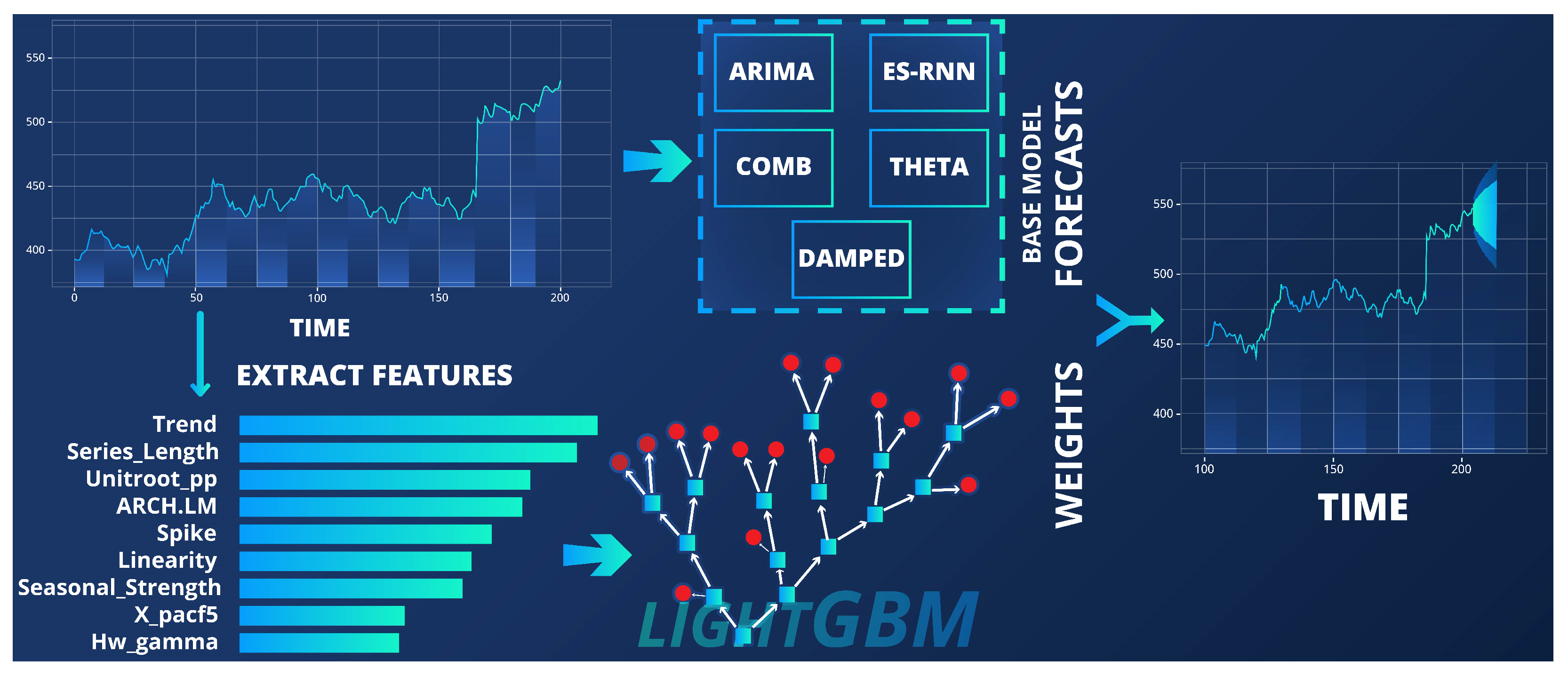
As a simple benchmark, this study implements a model averaging technique that averages the forecasts of the weak learners [53]. The combined forecast for a set of forecast models M might thus be expressed by the following notation:

$$\begin{array}{c}\hfill \widehat{y_t}=\frac{1}{n}·\sum _{m=1}^n{y}_{m_t},\end{array}$$

(11)

where n is the number of models in M and $y_{m_t}$ is the forecast of a model at time step t.

2.5. FFORMA

The FFORMA framework adopts a feature-weighted model averaging strategy [19]. A meta-learner learns how effectively a pool of forecasting models are at their task for different regions of the meta-feature space and then combines their predictions based on the learned model weightings. In addition, the FFORMA implements the gradient tree boosting model of an XGBoost, which the authors note is computationally efficient and has shown promising results for other problems [54].

Montero-Manso et al.’s [19] meta-learning methodology uses inputs of nine models and features extracted from the time-series, which measures the characteristics of a time-series: including, but not limited to, the features of lag, correlation, the strength of seasonality and spectral entropy.

Montero-Manso et al. [19] implement a custom objective function for the XGBoost to minimise. XGBoost requires both a gradient and hessian of the objective function to fit the model. The functions for their model are derived as follows. The term $p_m\left(f_n\right)$ is firstly defined as the output of the meta-learner for model m. A softmax transformation is applied to the numeric values to compute the model weights as the probability that each model is the best as:

$$\begin{array}{c}\hfill w_m\left(f_n\right)=\frac{\exp \left(p_m\left(f_n\right)\right)}{{\sum }_m\exp \left(p_m\left(f_n\right)\right)},\end{array}$$

(12)

where $w_m\left(f_n\right)$ is the weight produced by the GB meta-learner for base learner $m\in M$. For each n time-series, the contribution of each method for the OWA error is denoted as $L_{nm}$. The weighted average loss function is computed as:

$$\begin{array}{c}\hfill {\overline{L}}_n=\sum _{m=1}^M{w}_m\left(f_n\right)L_{nm},\end{array}$$

(13)

where ${\overline{L}}_n$ is the weighted average loss over the set of base learners M. The gradient of ${\overline{L}}_n$ is then computed as follows:

$$\begin{array}{c}\hfill G_{nm}=\frac{\partial {\overline{L}}_n}{\partial p_m\left(f_n\right)}=w_{nm}(L_{nm}-{\overline{L}}_n).\end{array}$$

(14)

The hessian of the objective function is then finally derived as follows:

$$\begin{array}{c}\hfill H_{nm}=\frac{\partial G_n}{\partial p_m\left(f_n\right)}\approx w_{nm}(L_{nm}(1-w_{nm})-G_{nm}).\end{array}$$

(15)

In order to minimise the objective function $\overline{L}$, the functions G and H are passed to XGBoost and the model’s hyperparameters are found using Bayesian optimisation on a limited search space that is determined based on preliminary results and rules of thumb.

Montero-Manso et al.’s [19] methodology combines the predictions of their pool of forecasting models using Algorithm 1. The forecasts are produced from the meta-learner’s estimated model weightings, given the meta-features of a new time-series. Thus, the fusion is achieved using the vector of weights $w\left(f_x\right)\in {\mathbb{R}}^M$ with a set of M forecasting models for each time-series x. Figure 2 depicts this experiment’s FFORMA forecasting pipeline.

Algorithm 1: FFORMA’s forecast combination [19]

The meta-feature for each time-series is computed by a function f. The FFORMA extracts 43 meta-features from each time-series using the R package called tsfeatures [55]. For nonseasonal time-series, features that only apply to seasonal time-series are set to zero. Unlike the ES-RNN, the domain-specific features supplied with the M4 dataset are not utilised in the FFORMA.

2.6. Random Forest Feature-Based FORecast Model Selection (FFORMS-R)

FFORMS-R, the precursor to FFORMA, learns to select a single model from a pool of forecasting models according to their varying performance observed over some meta-data feature space [56]. To this end, FFORMS-R uses a random forest ensemble learner [57] to classify a single model as the most relevant for some time-series features extracted from the reference series. Following the original FFORMS paper, we utilise the Gini impurity to determine the quality of a split. The same meta-features are used as per the FFORMA approach.

2.7. Gradient Boosting Feature-Based FORecast Model Selection (FFORMS-G)

The FFORMS-R framework demonstrates the benefit of selecting a single model from a pool of forecasting models [56]. We additionally propose replacing the weighted averaging of FFORMA with the selection of the model with the highest allocated weighting. This replacement allows us to compare how effective model selection is against weighted model averaging. This change is highlighted in Algorithm 1.

2.8. Neural Network Model Stacking (NN-STACK)

Cawood and van Zyl [1] proposed model stacking to conduct the forecasting of nonseasonal time-series. Their implementation performs regression over a feature space consisting of both the ensemble’s model forecasts and a set of statistics extracted from the time-series. This paper builds on their study by experimenting with more meta-features and a more extensive dataset of different domains and seasonalities.

The forecasts of a single timestep are combined using regression over both the ensemble’s base learner forecasts and the meta-features extracted from the input series. The MLP model performs regression over the inputs of the model forecasts and the extracted meta-features, with the target variables as the predicted series’ actual values. A neural network of a basic architecture is adopted, and each layer is transformed using the ReLU [58] activation function. The model is fit using mini-batches and the Adam [59] algorithm with a mean absolute error loss function.

This research extends the original NN-STACK implementation by including a more extensive set of meta-features for use by the FFORMA framework. Feature selection is achieved using the Spearman’s rank correlation coefficient ($\rho$) [60] of the meta-features’ correlation with the change in each model performance. This procedure helps reduce problems with overfitting, as only the most correlating features are included in the ensemble.

2.9. Neural Network Feature-Based FORecast Model Averaging (FFORMA-N)

We propose an additional MLP meta-learner that takes the time-series statistics as inputs and a one-hot encoded vector of the best performing model as the model’s target. The FFORMA-N is a deep learning approach to the FFORMA’s feature-weighted model averaging methodology. FFORMA-N adopts a softmax activation function in the MLP’s output layer to normalise the network’s output to a probability distribution, i.e., the probability of each base learner’s adequacy to model a time-series. The same meta-features and feature selection procedure are used as per the NN-STACK approach.

The neural network is of a deep architecture and adopts a ReLU activation function at each layer except for the softmax activated output layer. The model is fit using mini-batches and the Adam stochastic gradient descent algorithm with a categorical cross-entropy loss function.

The predictions of the forecasting models are combined, similar to the FFORMA’s fusion technique. The forecasts from the base learners are summed after they are weighted according to the meta-learner’s estimated probability distribution.

2.10. N-BEATS

Oreshkin et al. [33] reported a 3% accuracy improvement over the forecasts of the ES-RNN. We treat the N-BEATS method as a state-of-the-art benchmark to compare the performance of the ensembles. Therefore, the N-BEATS method is excluded from the ensembles’ pool of base learners. N-BEATS is a pure deep learning methodology that does not rely on feature engineering or input scaling [33].

3. Experimental Method and Results

All ensembles were evaluated using ten-fold cross-validation. This validation process was repeated five times, and the scores were averaged over all fifty validation sets to rule out chance from random initialisation. A pseudorandom number generator [61] was configured to produce the indices for splitting the data into the training and validation sets for each of the five runs. The seed numbers used were one, two, three, four and five.

All algorithms were implemented in Python and run on a 2.60 GHz Intel Core i7 PC with 16 GB RAM and 1365 MHz Nvidia RTX 2060 GPU with 6 GB GDDR6 memory. The source code of our experiments is available on GitHub (https://github.com/Pieter-Cawood/FFORMA-ESRNN accessed on 3 August 2022).

3.1. Hyperparameter Tuning

Subset names H, D, W, M, Y and Q in

Table 2. The FFORMA hyperparameters.

Hyperparameter	H	D	W	M	Y	Q
n-estimators	2000	2000	2000	1200	1200	2000
min data in leaf	63	200	50	100	100	50
number of leaves	135	94	19	110	110	94
eta	0.61	0.90	0.46	0.20	0.10	0.75
max depth	61	9	17	28	28	43
subsample	0.49	0.52	0.49	0.50	0.50	0.81
colsample bytree	0.90	0.49	0.90	0.50	0.50	0.49

,

Table 3. Average OWA errors on the M4 test set, where lower values are better.

	H (0.4K)	D (4.2K)	W (0.4K)	M (48K)	Y (23K)	Q (24K)	M, Y and Q
Base Learners
ARIMA	0.577	1.047	0.925	0.903	0.892	0.898	0.899
Comb	1.556	0.981	0.944	0.920	0.867	0.890	0.899
Damped	1.141	0.999	0.992	0.924	0.890	0.893	0.907
ES-RNN	0.440	1.046	0.864	0.836	0.778	0.847	0.825
Theta	1.006	0.998	0.965	0.907	0.872	0.917	0.901
Ensembles
FFORMA	0.415	0.983	0.725	0.800	0.732	0.816	0.788
FFORMS-R	0.423	0.981	0.740	0.817	0.752	0.830	0.805
FFORMS-G ${}^{‡}$	0.427	0.984	0.740	0.810	0.745	0.826	0.798
AVG	0.847	0.985	0.860	0.863	0.804	0.856	0.847
FFORMA-N ${}^{‡}$	0.428	0.979	0.718	0.813	0.746	0.828	0.801
NN-STACK	1.427	0.927	0.810	0.833	0.771	0.838	0.819
State of the Art
N-BEATS ${}^{†}$	-	-	-	0.819	0.758	0.800	0.799

^† reproduced for comparison [33], ^‡ proposed methods.

and

Table 4. Median OWA errors on the M4 test set, where lower values are better.

	H (0.4K)	D (4.2K)	W (0.4K)	M (48K)	Y (23K)	Q (24K)	Schulze Rank [63]
Base Learners
ARIMA	0.332	0.745	0.688	0.670	0.612	0.633	9
Comb	1.121	0.718	0.623	0.684	0.595	0.648	8
Damped	0.940	0.727	0.637	0.691	0.602	0.644	9
ES-RNN	0.370	0.764	0.546	0.637	0.550	0.610	5
Theta	0.817	0.723	0.673	0.692	0.617	0.686	11
Ensembles
FFORMA	0.318	0.723	0.529	0.602	0.491	0.580	1
FFORMS-R	0.311	0.711	0.552	0.615	0.511	0.589	2
FFORMS-G ${}^{‡}$	0.328	0.722	0.538	0.610	0.506	0.596	2
AVG	0.738	0.656	0.632	0.652	0.557	0.619	7
FFORMA-N ${}^{‡}$	0.326	0.720	0.539	0.614	0.508	0.594	2
NN-STACK	0.685	0.646	0.606	0.637	0.535	0.595	5

^‡ proposed methods.

correspond to the Hourly, Daily, Weekly, Monthly, Yearly and Quarterly data subsets. The ensembles’ architectures and hyperparameters were found using the training set of the first fold of the first cross-validation run. The two ensembles that use neural networks (NN-STACK and FFORMA-N) were tuned using backtesting, and the gradient boosting methods (FFORMA and FFORMS-G) were tuned using Bayesian optimisation. The parameter search space for the Bayesian optimisation was limited based on some initial results, and the Gaussian process method was configured to estimate the parameters that minimise the OWA error over 300 runs of parameter observations.

The FFORMA and FFORMS-G architecture and hyperparameters are identical and were automatically tuned using Bayesian optimisation over 300 runs of a limited parameter search space. For the model’s training, early stopping with patience ten was employed using the validation set loss. The validation set was a quarter of the training dataset. Table 2 presents the hyperparameter settings used to train the FFORMA ensembles for the M4 Competition’s dataset.

For FFORMS-R, we used the same hyperparameters to model all subsets of data. The forests were limited to 100 trees, with each tree having a maximum of sixteen nodes.

The NN-STACK’s architectures and hyperparameters were determined using backtesting on the training dataset of the first fold of the first run of cross-validation. The MLP architectures for the Hourly and Weekly subsets were deep with 11 hidden layers with neurons in each layer of (100, 100, 100, 100, 100, 50, 50, 50, 50, 20 and 20) sequentially. A more shallow network was used to model the Daily, Monthly, Yearly and Quarterly subsets with three hidden layers with ten neurons each.

Early stopping with patience 15 and a max epoch number of 300 was used, except for the Daily subset, which had a max epoch number of 600. All batch sizes were 225 except the Daily subset, set at 1200. Similarly, a learning rate of $0.0003$ was used everywhere except the Daily subset, which used $0.0001$.

Similar to the stacking method, the FFORMA-N’s architecture and hyperparameters were determined using backtesting on the training dataset of the first fold of the first run of cross-validation. The MLP architecture was deep, with 11 hidden layers with the numbers of neurons (100, 100, 100, 100, 100, 50, 50, 50, 50, 20 and 20) sequentially.

Early stopping was configured to terminate the training loop after a configured patience interval of three except for the in Daily subset, set at 15. A maximum number of epochs of 300 was used except for in the Daily subset in which the maximum was set to 600. All batch sizes were 52 except the Weekly subset at 225 and the Daily subset set at 1200. A learning rate of $0.0001$ was used throughout.

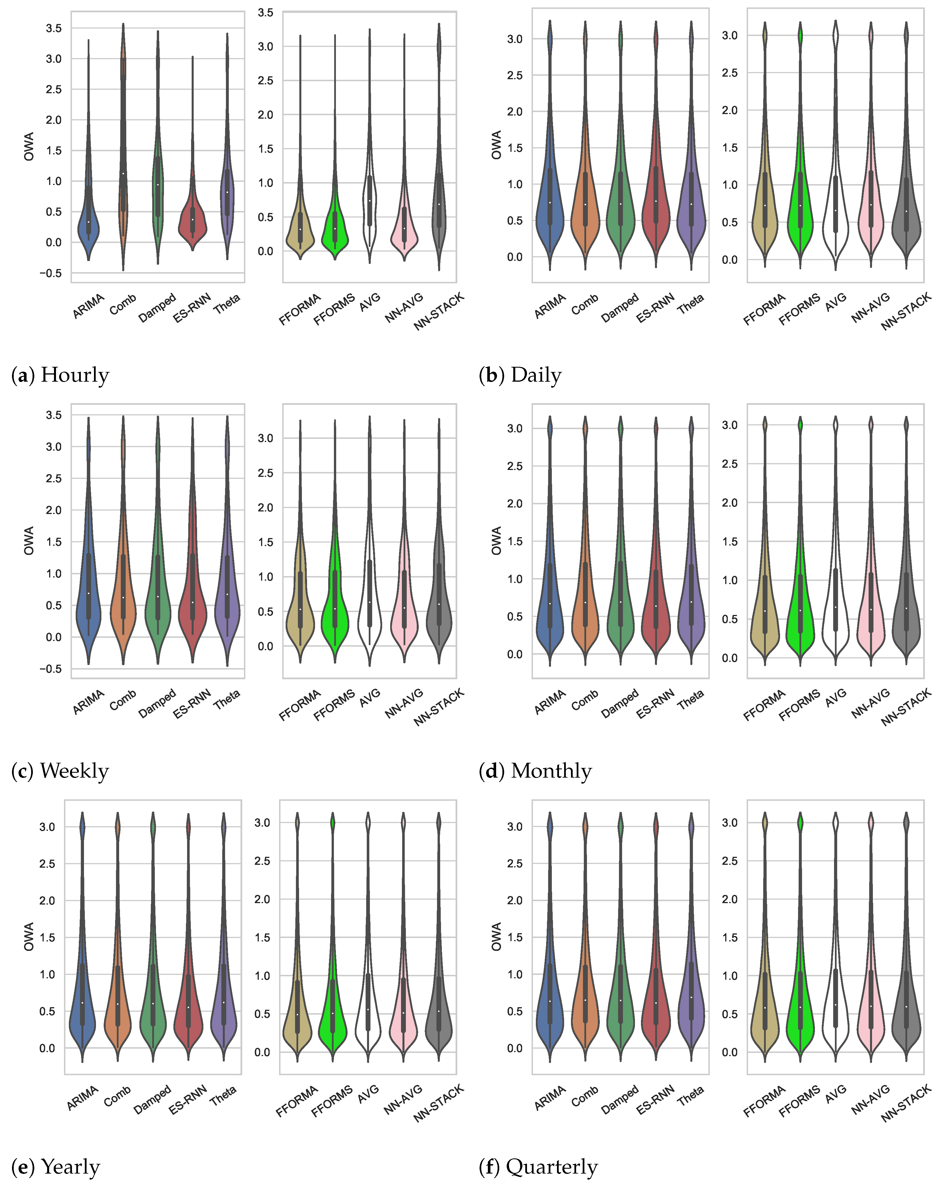
3.2. Detailed Results

Table 3 and Table 4 present the average and median OWA error performance for each forecasting method for each of the six data subsets of the M4 forecasting competition. Column “M, Y and Q” presents the mean over the three larger subsets. The inclusion of this mean is to provide a comparison to N-BEATS. The number of time-series of each data subset is provided in parentheses, the best results are given in bold, and the top two are highlighted in grey.

Egrioglu and Fildes [62] showed that the M4 competition’s ranking is flawed and that the average OWA error measurement is calculated from nonsymmetric error distributions and suggested that the errors should be ranked based on their median values instead. Egrioglu and Fildes [62] also argued that evaluating the combined results is of little value, as different methods are ranked best across different subsets. In order to present these more robust results, we present the median OWA errors in Table 4. In addition, Figure 3a–f depict the OWA error distributions and visualise the data quartiles and extreme values. The visualisations of the error distributions are used to analyse the consistency of each forecast method’s accuracy. The violin plots’ upper extreme values were clipped to $3.5$, a high OWA measurement representing model failure.

3.2.1. The Hourly Subset

For the Hourly subset, the ES-RNN produced the only stable forecasts amongst the pool of base learners (see Figure 3a). Subsequently, the NN-STACK failed as an ensembling method and produced the experiment’s worst average ensemble result. This failure was partly due to the small dataset (414 series) and the most extensive forecasting horizon requirement of 48 points.

The FFORMA outperformed all other forecasting methods and produced at least twice as much as the AVG benchmark. It was noted here that the ES-RNN’s median OWA error might slightly ($0.059$) be improved by utilising the hybrid model with the FFORMA ensemble technique.

3.2.2. The Daily Subset

The distributions of base learner errors (see Figure 3b) are exceptionally similar. Moreover, this was the only subset where the ES-RNN failed to outperform other base learners. Subsequently, the gradient boosting methods failed to gain the advantage of the ES-RNN’s forecasts as per the other subsets, and the NN-STACK method was the most successful ensemble and the best approach.

The results suggest that the NN-STACK method is a more suitable ensemble for situations where it is difficult for the ensemble to learn the weightings of superiority amongst the pool of similarly performing base learners.

3.2.3. The Weekly Subset

Considering the OWA distributions depicted in Figure 3c, the ES-RNN produced the lowest OWA errors amongst the other base learners, with considerably fewer forecasts reaching the extreme value of $3.0$. This exceptional performance of at least one base learner allowed all ensemble methods to outperform all base learners (see Table 3).

The FFORMA ensemble improved the ES-RNN’s median OWA error by a small ($0.017$) margin. The FFORMA performed the best of all methods, whereas the FFORMS-G was the second-best.

3.2.4. The Monthly Subset

The Monthly subset consisted of 48,000 time-series and was the largest and most domain-balanced dataset of all the experiments. Figure 3d depicts the distribution of the OWA errors, and the ES-RNN performed best amongst the base learners, with a notably smaller number of model failures. These conditions are ideal for analysing the general performance of the ensemble methods, and the results show similar performance in median OWA errors and a slight ($0.037$) improvement when the FFORMA learns from the predictions of the ES-RNN. Nevertheless, considering the median OWA error, the FFORMA remained the superior method and outperformed all other approaches.

3.2.5. The Yearly Subset

The Yearly subset was one of the experiment’s larger and nonseasonal datasets. It was noted that all ensembles, except for the AVG benchmark, slightly outperformed the ES-RNN. Similar OWA distributions were observed between the gradient boosting and neural network ensembles (see Figure 3e) However, the FFORMA showed the greatest ($0.056$) improvement, and it is the preferred ensemble for time-series with a Yearly seasonality.

3.2.6. The Quarterly Subset

The Quarterly subset was similar to the Yearly one in size, balance and forecast horizon. The only exception is that the Quarterly time-series contained a higher seasonality. Considering the ensembles’ OWA distributions visualised in Figure 3f, similar ensembling performance was observed to that of the ensembling performance on the Yearly subset. Likewise, no base learner was distinguishable in terms of the OWA distributions. However, the more extensive dataset allowed the ensemble methods to avoid the case of the minor Daily dataset (with similar performing base learners), and the FFORMA ensemble produced a $0.03$ improvement over the median accuracy of the ES-RNN.

The N-BEATS approach showed the best average OWA result, and it was able to outperform the FFORMA for this subset only by a small margin of $0.058$.

3.3. Overall Results

N-BEATS outperformed all other ensembles only for the Quarterly subset. Therefore, the utility of N-BEATS might have notably boosted the ensembles’ accuracy for the Quarterly subset. The median OWA error gap between the AVG and other ensemble methods (e.g., between the FFORMA: $0.101$) indicates that machine learning is a robust solution to late data fusion.

Although all the ensembles outperformed both the ES-RNN’s and N-Beats average error when considering the OWA error distributions (Figure 3d–f of the three larger subsets (Monthly, Yearly and Quarterly), there is still generally a large amount of uncertainty when considering the (Hourly, Daily and Weekly) datasets. Nevertheless, the ensembles were still able to lower the upper quantiles of the OWA error distributions by a notable margin. A more significant improvement was observed in the OWA error distributions of the three smaller subsets (Hourly, Daily and Weekly) (see Figure 3a,b, where the weak learners showed more remarkable performance (considering their OWA errors.)

The outstanding ensemble learning performance by both our presented methods and previously by N-BEATS provides evidence that:

1.

The performance of ensemble learning is dependent on the performances of its weak learners;

2.

Ensemble learning’s performance is dependent on the diversity of the data (i.e., the similarity of the time-series from the different domains);

3.

For smaller subsets, the traditional methods do better but are still outperformed by the ensemble methods and even more so for larger datasets, where more cross-learning can be exploited;

4.

The ensembles of hybrids can still lead to improved performance;

5.

We reaffirm that there is no free lunch concerning the selection of ensembling methods and that validation will still be required for model selection.

When considering the ensemble learning methods, we note that the gradient boosting ensembles generally outperformed those of neural networks. Furthermore, both gradient boosting ensembles outperformed all other ensemble methods on all subsets except for the Daily subset. Table 4 statistically shows that for all datasets, it is always possible to improve a standalone time-series forecast model by adding it to an ensemble with other statistical forecast models. Lastly, since the FFORMA (the second-place M4 submission) utilises the ES-RNN as a base learner, the FFORMA could outperform the standalone ES-RNN (the M4 winner) for all six subsets of data.

4. Conclusions

Our primary objective was to empirically compare ensemble methods against the state-of-the-art forecasting methods, the ES-RNN and N-BEATS, to determine whether we might (i) boost the accuracy of contemporary hybrid models and (ii) single out a method as the state-of-the-art ensembling technique for future research efforts.

The experiment included four traditional base learners, namely ARIMA, Comb, Damped and Theta, and an advanced and hybrid machine learning model, the ES-RNN. The ensembles of the experiment adopt different ensembling strategies of model averaging, stacking and selection. We experimented with a random forest meta-learner, namely the FFORMS-R, two gradient boosting ones, namely the FFORMA and FFORMS-G, two neural network approaches, namely NN-STACK and FFORMA-N, and a naive arithmetic average as a benchmark. We additionally compared the results of the state-of-the-art benchmark, namely N-BEATS, using the results reported in their paper.

Regarding the obtained results, we show that the FFORMA is a state-of-the-art ensemble technique that might be used to boost the predictive power of powerful methods such as the ES-RNN and N-BEATS. However, considering the case of the Daily subset, the NN-STACK approach might be a more suitable ensemble when the pool of forecasting models has similar performance. Further, we show that weighted model averaging is a superior ensemble approach, as both the FFORMA and FFORMA-N generally outperform versions of their same architecture that perform model stacking or selection.

NN-STACK performs regression over single points of the base learner forecasts. NN-STACK, therefore, ignores the temporal element of the data, and the meta-learner instead learns a temporally blind fusion function. Consequently, we recommend that future research consider investigating the performance of a stacking ensemble that is conscious of the data’s temporality. Furthermore, considering the equal-weighted averaging adopted by the top submissions of the M5 Competition, further research is needed to assess the performance of feature-weighted model averaging for multivariate time-series data.

References

1. Cawood, P.; van Zyl, T.L. Feature-weighted stacking for nonseasonal time series forecasts: A case study of the COVID-19 epidemic curves. In Proceedings of the 2021 8th International Conference on Soft Computing Machine Intelligence (ISCMI), Cario, Egypt, 26–27 November 2021; pp. 53–59. [Google Scholar]
2. Makridakis, S.; Hyndman, R.J.; Petropoulos, F. Forecasting in social settings: The state of the art. Int. J. Forecast. 2020, 36, 15–28. [Google Scholar] [CrossRef]
3. Atherfold, J.; Van Zyl, T. A method for dissolved gas forecasting in power transformers using ls-svm. In Proceedings of the 2020 IEEE 23rd International Conference On Information Fusion (FUSION), Rustenburg, South Africa, 6–9 July 2020; pp. 1–8. [Google Scholar]
4. Mathonsi, T.; Zyl, T. Multivariate anomaly detection based on prediction intervals constructed using deep learning. In Proceedings of the Neural Computing And Applications, Jinan, China, 8–10 July 2022; pp. 1–15. [Google Scholar]
5. Timilehin, O.; Zyl, T. Surrogate Parameters Optimization for Data and Model Fusion of COVID-19 Time-series Data. In Proceedings of the 2021 IEEE 24th International Conference On Information Fusion (FUSION), Sun City, South Africa, 1–4 November 2021; pp. 1–7. [Google Scholar]
6. Freeborough, W.; Zyl, T. Investigating Explainability Methods in Recurrent Neural Network Architectures for Financial Time Series Data. Appl. Sci. 2022, 12, 1427. [Google Scholar] [CrossRef]
7. Michelsanti, D.; Tan, Z.H.; Zhang, S.X.; Xu, Y.; Yu, M.; Yu, D.; Jensen, J. An overview of deep-learning-based audio-visual speech enhancement and separation. IEEE/ACM Trans. Audio Speech Lang. Process. 2021, 29, 1368–1396. [Google Scholar] [CrossRef]
8. Arinze, B. Selecting appropriate forecasting models using rule induction. Omega 1994, 22, 647–658. [Google Scholar] [CrossRef]
9. Ribeiro, M.H.D.M.; Coelho, L.D.S. Ensemble approach based on bagging, boosting and stacking for short-term prediction in agribusiness time series. Appl. Soft Comput. 2020, 86, 105837. [Google Scholar] [CrossRef]
10. Zhang, G.P. Time series forecasting using a hybrid arima and neural network model. Neurocomputing 2003, 50, 159–175. [Google Scholar] [CrossRef]
11. Wolpert, D.H.; Macready, W.G. No free lunch theorems for optimization. IEEE Trans. Evol. Comput. 1997, 1, 67–82. [Google Scholar] [CrossRef]
12. Reich, N.G.; Brooks, L.C.; Fox, S.J.; Kandula, S.; McGowan, C.J.; Moore, E.; Osthus, D.; Ray, E.L.; Tushar, A.; Yamana, T.K.; et al. A collaborative multiyear, multimodel assessment of seasonal influenza forecasting in the united states. Proc. Natl. Acad. Sci. USA 2019, 116, 3146–3154. [Google Scholar] [CrossRef]
13. McGowan, C.J.; Biggerstaff, M.; Johansson, M.; Apfeldorf, K.M.; Ben-Nun, M.; Brooks, L.; Convertino, M.; Erraguntla, M.; Farrow, D.C.; Freeze, J.; et al. Collaborative efforts to forecast seasonal influenza in the united states, 2015–2016. Sci. Rep. 2019, 9, 683. [Google Scholar] [CrossRef]
14. Johansson, M.A.; Apfeldorf, K.M.; Dobson, S.; Devita, J.; Buczak, A.L.; Baugher, B.; Moniz, L.J.; Bagley, T.; Babin, S.M.; Guven, E.; et al. An open challenge to advance probabilistic forecasting for dengue epidemics. Proc. Natl. Acad. Sci. USA 2019, 116, 24268–24274. [Google Scholar] [CrossRef]
15. Raftery, A.E.; Madigan, D.; Hoeting, J.A. Bayesian model averaging for linear regression models. J. Am. Stat. Assoc. 1997, 92, 179–191. [Google Scholar] [CrossRef]
16. Clarke, B. Comparing bayes model averaging and stacking when model approximation error cannot be ignored. J. Mach. Learn. Res. 2003, 4, 683–712. [Google Scholar]
17. Lorena, A.C.; Maciel, A.I.; de Miranda, P.B.; Costa, I.G.; Prudêncio, R.B. Data complexity meta-features for regression problems. Mach. Learn. 2018, 107, 209–246. [Google Scholar] [CrossRef]
18. Barak, S.; Nasiri, M.; Rostamzadeh, M. Time series model selection with a meta-learning approach; evidence from a pool of forecasting algorithms. arXiv 2019, arXiv:1908.08489. [Google Scholar]
19. Montero-Manso, P.; Athanasopoulos, G.; Hyndman, R.J.; Talagala, T.S. Fforma: Feature-based forecast model averaging. Int. J. Forecast 2020, 36, 86–92. [Google Scholar] [CrossRef]
20. Smyl, S. A hybrid method of exponential smoothing and recurrent neural networks for time series forecasting. Int. J. Forecast 2020, 36, 75–85. [Google Scholar] [CrossRef]
21. Liu, N.; Tang, Q.; Zhang, J.; Fan, W.; Liu, J. A hybrid forecasting model with parameter optimization for short-term load forecasting of micro-grids. Appl. Energy 2014, 129, 336–345. [Google Scholar] [CrossRef]
22. Wang, J.-Z.; Wang, Y.; Jiang, P. The study and application of a novel hybrid forecasting model—A case study of wind speed forecasting in china. Appl. Energy 2015, 143, 472–488. [Google Scholar] [CrossRef]
23. Qin, Y.; Li, K.; Liang, Z.; Lee, B.; Zhang, F.; Gu, Y.; Zhang, L.; Wu, F.; Rodriguez, D. Hybrid forecasting model based on long short term memory network and deep learning neural network for wind signal. Appl. Energy 2019, 236, 262–272. [Google Scholar] [CrossRef]
24. Mathonsi, T.; van Zyl, T.L. Prediction interval construction for multivariate point forecasts using deep learning. In Proceedings of the 2020 7th International Conference on Soft Computing & Machine Intelligence (ISCMI), Stockholm, Sweden, 14–15 November 2020; pp. 88–95. [Google Scholar]
25. Laher, S.; Paskaramoorthy, A.; Zyl, T.L.V. Deep learning for financial time series forecast fusion and optimal portfolio rebalancing. In Proceedings of the 2021 IEEE 24th International Conference on Information Fusion (FUSION), Sun City, South Africa, 1–4 November 2021; pp. 1–8. [Google Scholar]
26. Mathonsi, T.; van Zyl, T.L. A statistics and deep learning hybrid method for multivariate time series forecasting and mortality modeling. Forecasting 2022, 4, 1–25. [Google Scholar] [CrossRef]
27. Zhang, G.; Patuwo, B.E.; Hu, M.Y. Forecasting with artificial neural networks: The state of the art. Int. J. Forecast. 1998, 14, 35–62. [Google Scholar] [CrossRef]
28. Aksoy, A.; Öztürk, N.; Sucky, E. Demand forecasting for apparel manufacturers by using neuro-fuzzy techniques. J. Model. Manag. 2014, 9, 918–935. [Google Scholar] [CrossRef]
29. Deng, W.; Wang, G.; Zhang, X. A novel hybrid water quality time series prediction method based on cloud model and fuzzy forecasting. Chemom. Intell. Lab. Syst. 2015, 149, 39–49. [Google Scholar] [CrossRef]
30. Rahmani, R.; Yusof, R.; Seyedmahmoudian, M.; Mekhilef, S. Hybrid technique of ant colony and particle swarm optimization for short term wind energy forecasting. J. Wind. Eng. Ind. Aerodyn. 2013, 123, 163–170. [Google Scholar] [CrossRef]
31. Kumar, S.; Pal, S.K.; Singh, R. A novel hybrid model based on particle swarm optimisation and extreme learning machine for short-term temperature prediction using ambient sensors. Sustain. Cities Soc. 2019, 49, 101601. [Google Scholar] [CrossRef]
32. Shinde, G.R.; Kalamkar, A.B.; Mahalle, P.N.; Dey, N.; Chaki, J.; Hassanien, A.E. Forecasting models for coronavirus disease (COVID-19): A survey of the state-of-the-art. SN Comput. Sci. 2020, 1, 197. [Google Scholar] [CrossRef]
33. Oreshkin, B.N.; Carpov, D.; Chapados, N.; Bengio, Y. N-beats: Neural basis expansion analysis for interpretable time series forecasting. arXiv 2019, arXiv:1905.10437. [Google Scholar]
34. Huang, G.; Liu, Z.; Maaten, L.V.D.; Weinberger, K.Q. Densely connected convolutional networks. In Proceedings of the IEEE Conference on Computer Vision and Pattern Recognition, Honolulu, HI, USA, 21–26 July 2017; pp. 4700–4708. [Google Scholar]
35. Makridakis, S.; Spiliotis, E.; Assimakopoulos, V. The m5 competition: Background, organization, and implementation. Int. J. Forecast. 2021. [Google Scholar] [CrossRef]
36. Makridakis, S.; Spiliotis, E.; Assimakopoulos, V. The m4 competition: 100,000 time series and 61 forecasting methods. Int. J. Forecast. 2020, 36, 54–74. [Google Scholar] [CrossRef]
37. Makridakis, S.; Spiliotis, E.; Assimakopoulos, V. M5 accuracy competition: Results, findings, and conclusions. Int. J. Forecast. 2022. [Google Scholar] [CrossRef]
38. Rokach, L. Ensemble-based classifiers. Artif. Intell. Rev. 2010, 33, 1–39. [Google Scholar] [CrossRef]
39. Wu, Q. A hybrid-forecasting model based on gaussian support vector machine and chaotic particle swarm optimization. Expert Syst. Appl. 2010, 37, 2388–2394. [Google Scholar] [CrossRef]
40. Khashei, M.; Bijari, M. A new class of hybrid models for time series forecasting. Expert Syst. Appl. 2012, 39, 4344–4357. [Google Scholar]
41. Makridakis, S. Accuracy measures: Theoretical and practical concerns. Int. J. Forecast. 1993, 9, 527–529. [Google Scholar] [CrossRef]
42. Hyndman, R.J.; Koehler, A.B. Another look at measures of forecast accuracy. Int. J. Forecast. 2006, 22, 679–688. [Google Scholar] [CrossRef]
43. Hyndman, R.J.; Khandakar, Y. Automatic time series forecasting: The forecast package for r. J. Stat. Softw. 2008, 27, 1–22. [Google Scholar] [CrossRef]
44. Assimakopoulos, V.; Nikolopoulos, K. The theta model: A decomposition approach to forecasting. Int. J. Forecast. 2000, 16, 521–530. [Google Scholar] [CrossRef]
45. Holt, C.C. Forecasting seasonals and trends by exponentially weighted moving averages. Int. J. Forecast. 2004, 20, 5–10. [Google Scholar] [CrossRef]
46. McKenzie, E.; Gardner, E.S., Jr. Damped trend exponential smoothing: A modelling viewpoint. Int. J. Forecast. 2010, 26, 661–665. [Google Scholar] [CrossRef]
47. Makridakis, S.; Hibon, M. The m3-competition: Results, conclusions and implications. Int. J. Forecast. 2000, 16, 451–476. [Google Scholar] [CrossRef]
48. Fathi, O. Time series forecasting using a hybrid arima and lstm model. Velv. Consult. 2019, 1–7. Available online: https://www.velvetconsulting.com/nos-publications2/time-series-forecasting-using-a-hybrid-arima-and-lstm-model/ (accessed on 7 June 2022).
49. Petropoulos, F.; Hyndman, R.J.; Bergmeir, C. Exploring the sources of uncertainty: Why does bagging for time series forecasting work? Eur. J. Oper. Res. 2018, 268, 545–554. [Google Scholar] [CrossRef]
50. Chan, F.; Pauwels, L.L. Some theoretical results on forecast combinations. Int. J. Forecast. 2018, 34, 64–74. [Google Scholar] [CrossRef]
51. Gardner, E.S., Jr. Exponential smoothing: The state of the art. J. Forecast. 1985, 4, 1–28. [Google Scholar] [CrossRef]
52. Chang, S.; Zhang, Y.; Han, W.; Yu, M.; Guo, X.; Tan, W.; Cui, X.; Witbrock, M.; Hasegawa-Johnson, M.; Huang, T.S. Dilated recurrent neural networks. arXiv 2017, arXiv:1710.02224. [Google Scholar]
53. Claeskens, G.; Hjort, N.L. Model Selection and Model Averaging; Cambridge University Press: Cambridge, UK, 2008. [Google Scholar]
54. Chen, T.; Guestrin, C. Xgboost: A scalable tree boosting system. In Proceedings of the 22nd ACM Sigkdd International Conference on Knowledge Discovery and Data Mining, San Francisco, CA, USA, 13–17 August 2016; pp. 785–794. [Google Scholar]
55. Hyndman, R.J.; Wang, E.; Laptev, N. Large-scale unusual time series detection. In Proceedings of the 2015 IEEE International Conference on Data Mining Workshop (ICDMW), Atlantic City, NJ, USA, 14–17 November 2015; pp. 1616–1619. [Google Scholar]
56. Talagala, T.S.; Hyndman, R.J.; Athanasopoulos, G. Meta-learning how to forecast time series. Monash Econom. Bus. Stat. Work. Pap. 2018, 6, 18. [Google Scholar]
57. Liaw, A.; Wiener, M. Classification and regression by randomforest. R News 2002, 2, 18–22. [Google Scholar]
58. Agarap, A.F. Deep learning using rectified linear units (relu). arXiv 2018, arXiv:1803.08375. [Google Scholar]
59. Kingma, D.P.; Ba, J. Adam: A method for stochastic optimization. arXiv 2014, arXiv:1412.6980. [Google Scholar]
60. Zar, J.H. Spearman rank correlation. Encycl. Biostat. 2005, 7. [Google Scholar] [CrossRef]
61. Blum, L.; Blum, M.; Shub, M. A simple unpredictable pseudo-random number generator. SIAM J. Comput. 1986, 15, 364–383. [Google Scholar] [CrossRef]
62. Egrioglu, E.; Fİldes, R. A note on the robustness of performance of methods and rankings for m4 competition. Turk. J. Forecast. 2020, 4, 26–32. [Google Scholar]
63. Schulze, M. The Schulze method of voting. arXiv 2018, arXiv:1804.02973. [Google Scholar]
Figure 1. An incomplete taxonomy of model fusion showing ensemble learning, boosting, parallel ensembles, stacking, deep learning, and hybrid models [9,10].
Forecasting 04 00040 g001
Figure 2. The FFORMA forecasting pipeline.
Forecasting 04 00040 g002
Figure 3. The OWA error distributions on the M4 test set, where FFORMS represents the similar distributions of FFORMS-R and FFORMS-G. Where (a) shows the distributions for the Hourly subset, (b) the Daily subset, (c) the Weekly subset, (d) the Monthly subset (e) the Yearly subset and (f) the Quarterly subset.
Forecasting 04 00040 g003