Assessing the Implication of Climate Change to Forecast Future Flood Using CMIP6 Climate Projections and HEC-RAS Modeling

Abstract

Climate change has caused uncertainty in the hydrological pattern including weather change, precipitation fluctuations, and extreme temperature, thus triggering unforeseen natural tragedies such as hurricanes, flash flooding, heatwave and more. Because of these unanticipated events occurring all around the globe, the study of the influence of climate change on the alteration of flooding patterns has gained a lot of attention. This research study intends to provide an insight into how the future projected streamflow will affect the flooding-inundation extent by comparing the change in floodplain using both historical and future simulated scenarios. For the future projected data, the climate model Atmosphere/Ocean General Circulation Model (AOGCM) developed by Coupled Model Intercomparison Project Phase 6 (CMIP6) is used, which illustrates that the flood is increasing in considering climate models. Furthermore, a comparison of the existing flood inundation map by the Federal Emergency Management Agency (FEMA) study with the map generated by future projected streamflow data presents the entire inundation area in flood maps, implying the expansion area compared to FEMA needs to be considered in making emergency response plans. The effect of flooding in the inundation area from historical to future flow values, presented mathematically by a calculation of inundation extent percentage, infers that the considered watershed of Rock River is a flood-prone area. The goal is to provide insights on the importance of using the forecasted data for flood analysis and to offer the necessary background needed to strategize an emergency response plan for flood management.

1. Introduction

Regarding the Third National Climate Assessment, in the last fifty years, the United States has been experiencing an elongated period of outrageous high temperatures, excessive downpours, and alarming floods and drought. Climate change due to anthropogenic activities is primarily due to increases in concentrations of greenhouse gas emissions [1,2]. This issue has escalated, and there has been an increase in temperature. The increase in temperature has caused significant variation of precipitation and evaporation both temporally and spatially [3,4]. Rainfall patterns have been altered due to these changes, which have had implications for water resources [5]. Studies insights that on average there is rise in sea level about 3.7 mm/yr from 2006 to 2018 [6]. Unexpected floods have been recorded in several regions because of the rising levels in water resources [7,8].

The damages caused by the flooding event in economic, social and environmental aspects necessitates estimations of floods and the area of extent that they will damage in the future due to climate change [9]. The change in hydrological features is causing a cascading effect on the streamflow regime throughout the world, and already, such implications in the form of drought and flood are being experienced [10]. This is the reason governments, researchers, engineers and utilities are diverting their attention to quantifying the climate change influence on future flood risk so that they can be better prepared with robust strategies to adapt to climate change and make informed decision about mitigation strategies [11,12].

To amplify climate-related research, the World Climate Research Programme (WCRP) launched the Coupled Model Intercomparison Project (CMIP) in 1995 [13]. The climate models, commonly known as the General Circulation Models (GCMs), have been in constant development by different hydrological research communities to understand the hydro-climatological phenomenon due to the change in climate. The Atmosphere/Ocean General Circulation Model (AOGCM) is the established global model developed at the Global Modeling and Assimilation Office. By simulating the mean climate and inter-annual climate variability, model performance is evaluated [14]. AOGCM has a significant description of the large-scale atmospheric balances of momentum, heat and moisture. The model uses large sets of equations to approximate the small-scale processes such as precipitation and heat exchange with sea surface and land [15]. This study considers the AOGCM based on the availability of data, details of which are explained in upcoming sections.

Starting from CMIP1 [16] and CMIP2, the CMIP model continues its progress with CMIP3 [17,18], CMIP5 [19,20,21], and now, CMIP6 [13]. CMIP5 presented Representative Concentration Pathways (RCPs), which included greenhouse gas emission scenarios that are likely to happen in the future. The name of the scenario was coined based on possible radioactive forcing values (Wm⁻²) at the end of this century as compared to pre-industrial times, which included RCP2.6, RCP4.5, RCP6.0, and RCP8.5, each denoting the amount of radioactive values equal to the numeric content of the RCPs [22,23]. Past research has used the CMIP5 dataset to explore extreme hydrological projections in the future if these values are considered and has performed rainfall-runoff analysis, comparison-based study, and hydro-climatic study [24,25,26,27,28]. The CMIP5 model with RCPs, however, suggested a significant decrease in aerosol emission by the end of the century [29] and lacked the incorporation of socio-economic factors that led to the development of CMIP6 model. The recent development of the model CMIP6 has Scenario Model Intercomparison Project (ScenarioMIP) as a key activity [30]. This version proposes shared socioeconomic pathways (SSPs), which reflect a variety of scenarios for greenhouse gas emission and land use change, incorporating socio-economic factors such as urban development, economic progression, climate mitigation initiatives, educational and technological development, and global policies computed by integrated assessment models [30]. The CMIP6 model has gained popularity in determining changes in hydrological parameters such as precipitation and temperature in the future [31,32], assessing the risk posed by the climate projected runoff values to the areas [33,34], comparisons of different climate scenarios [35,36,37], and so on. In addition, the CMIP6 version has river discharge as one of the parameters, and the use of this variable has not been given much attention by prior research, and so this research studies the change in river discharge due to climate change based on the CMIP6 model.

The climate model dataset from CMIP6 gives the future projected data for the river discharge. However, we need to visualize the flood extend corresponding to the given streamflow data. For this purpose, flood inundation mapping is popularly considered for proper management of flooding and delineating the flood extend area [38]. This study uses Hydrological Engineering Center’s River Analysis System (HEC-RAS developed by USACE HEC, Davis, CA, USA) model for flood inundation mapping and further inundation analysis. HEC-RAS is standard software for hydraulic modeling, which was developed by the U.S. Army Corps of Engineers. This model has been adopted by past research literature for flood inundation mapping [39], flood hazard assessment [40], and flood risk assessment [41].

The proposed study is based on the watershed of Rock River. The change in flood regime in the particular stretch of Rock River makes it a good fit to explain the research’s objective. In addition, future floodplain analysis in the case of a meandering river stretch has always been a challenge [42,43]. In this regard, the meanderings always provide a good example of the research. The research study presents the appropriateness of the bias correction method for finalizing the flow data and validating the flood model output with the Federal Emergency Management Agency (FEMA) map to show the used model’s effectiveness in meandering rivers. So, similar models can be used for the analysis of similar other rivers. CMIP6 is considered in the case of CMIP5 due to improved data of non-bias-corrected CMIP6 rather than non-bias-corrected CMIP5 [36]. The study also presents the calculation of inundation extent and asserts its results.

This study focuses on the use of CMIP6 scenario-based streamflow datasets for flood forecasting. The examination of climate change impact is performed by comparing the current flooding for different return periods with the future projected scenarios by analyzing the floodplain mapping in both instances and calculating the inundation extent for the given context. This research study ponders the watershed of Rock River to further elucidate the need for flood forecasting to plan long-lasting management strategies. The novelty of this study is that it explores the inundation extent in current and future scenarios to provide in-depth insight into the implications of not employing flood projected data. The objectives of the research are:

• To understand the impact of climate model in future runoff values and flood frequency.
• To evaluate the change in the inundation area for different value of discharge for a particular frequency.
• To assess the area that FEMA can consider for making quick response plan, considering the future projected runoff value from the climate change.
• To signify the representation of the computed inundation extent value.

Based on the current research, it is expected to emphasize the need of preparing responsive actions using projected future data sets. This is accomplished by comparing the inundation extent to convey the fact that present databases underestimate the inundation area for extreme occurrences, and that utilizing these data for the planning phase might not always be particularly useful considering future flooding growth.

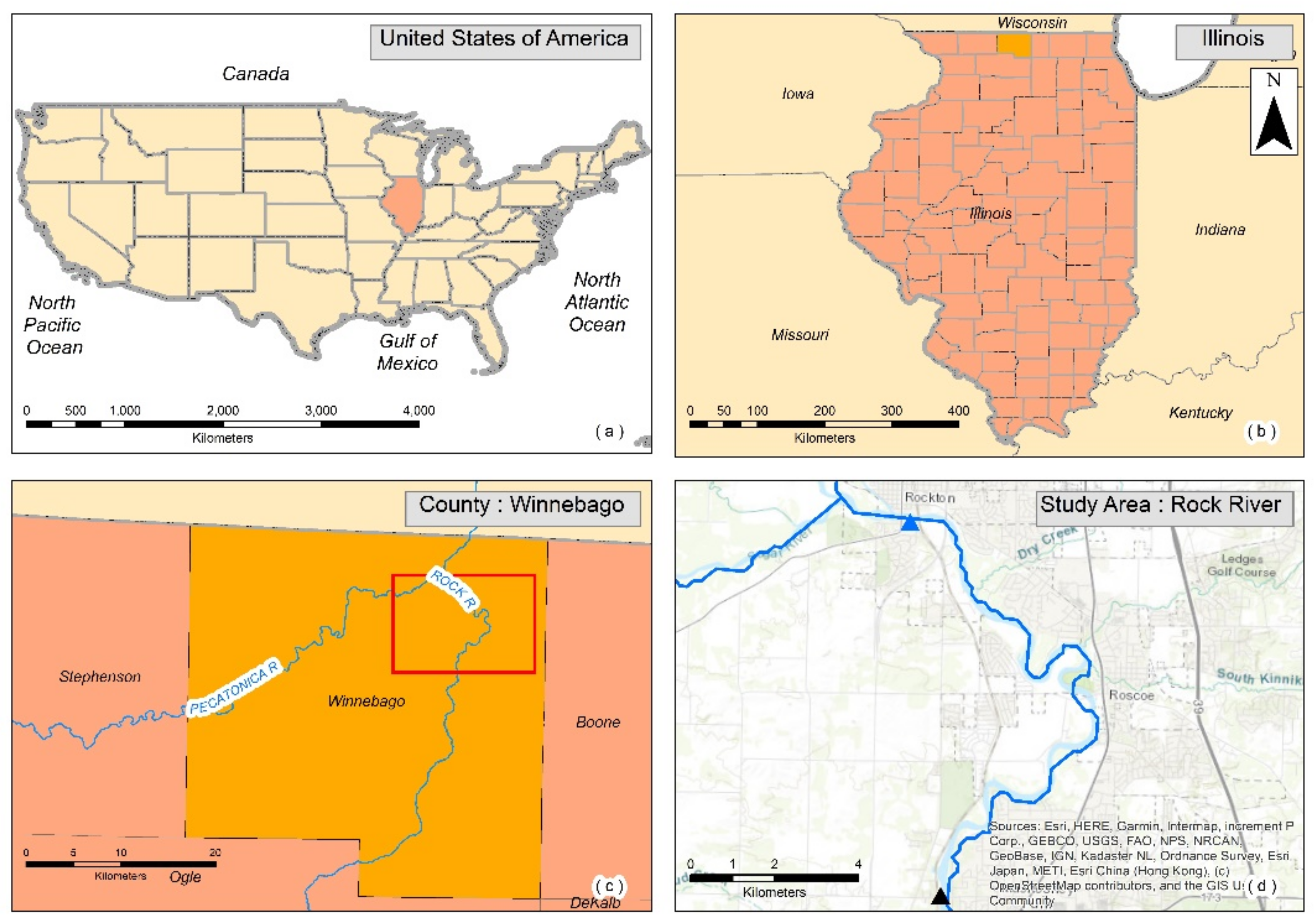
2. Study Area

The study area is within the reach of Rock River, located in north-central United States, which flows from Horicon Marsh near Brandon in Fond du Lac County in a southwest direction, joining Mississippi River at Rock Island, Illinois. The lower course bottomland of this river reach is prone to spring flooding, necessitating levee protection. Our research region extends from Rockton city at the upstream to Machesney Park at the downstream, as seen in Figure 1. These places also serve as the United States Geological Survey (USGS) gage station sites, with the upstream station (Station ID 05437500) located at 42°27′01″ N, 89°04′21″ W with an elevation of 215.72 m above NAVD88 and the downstream station (Station ID 05437610) located at 42°22′08″ N, 89°03′31″ W with an elevation of 212.95 m above NAVD88. The reach of the study area is 20.72 km long. The watershed area of the river at the upstream station is approximately 16,480 km². The gage station discharge data from the upstream are used as observed data for bias-correcting the climate model data, and the gage station gage height data are used for the calibration and validation of hydrologic modelling using HEC-RAS. Details about these steps are further explained in sections below. The site has suffered from spring flooding mainly due to unexpected precipitation. The most recent flood event in Machesney Park was in 2019, due to the combination of sleet and freezing rain. This study further uses the Flood Insurance Map developed by FEMA at this site to validate the HEC-RAS model and compare the inundation extend with future projected data.

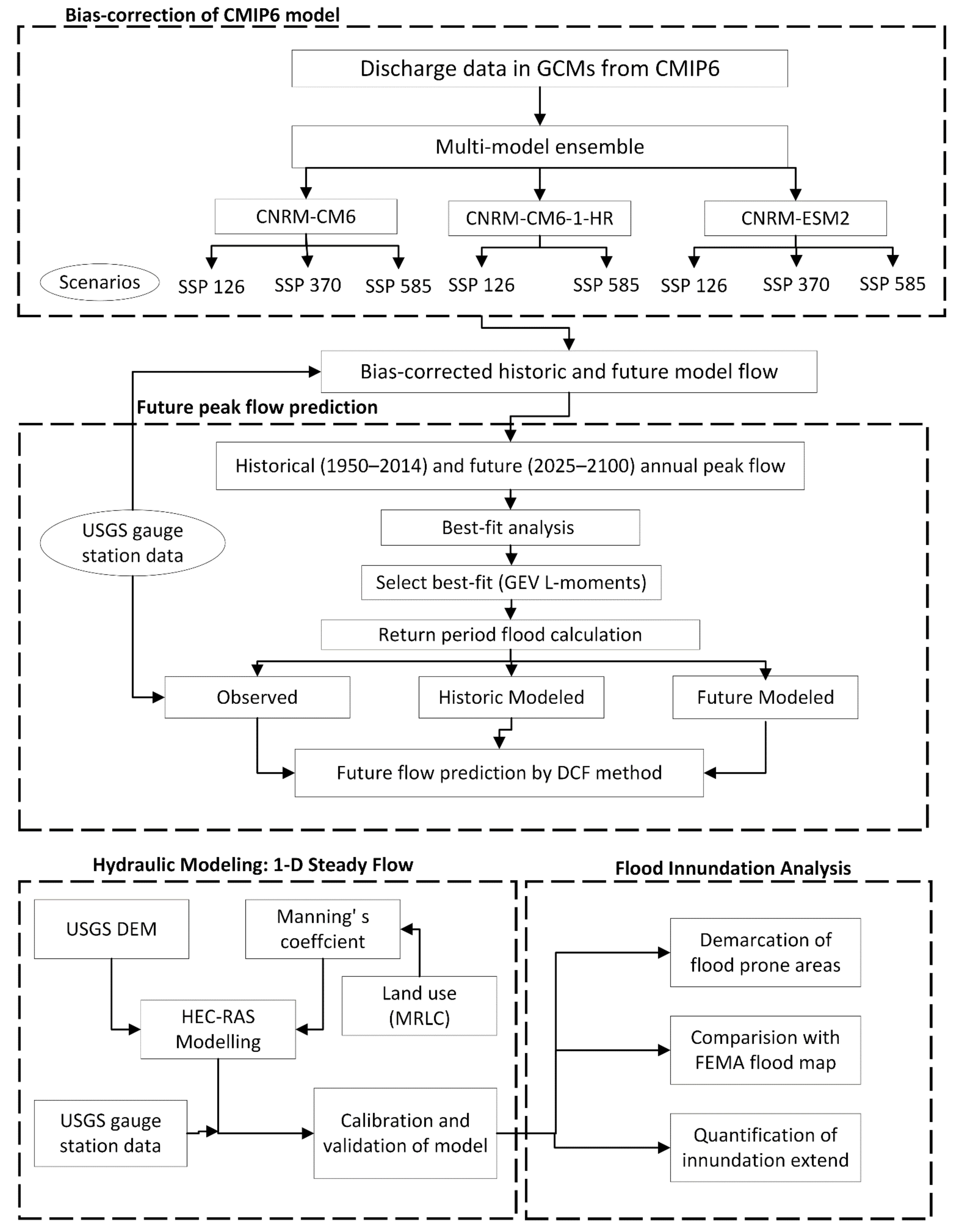
3. Methodology

The study considers the understanding of the Global Climate Models (GCMs) and Coupled Model Intercomparison Project (CMIP 6) for the change in floodplain area in the future in the area around Rock River. The methodology involves the runoff data extraction and correction over the carbon emissions scenarios driven by various Shared Socioeconomic Pathways data, historical and future data comparison, inundation modelling, verification of gage height from the Gage Station defined in United States Geological Survey (USGS) and model in Hydrological Engineering Centre—River Analysis System (HEC-RAS), and comparison of flood plain from the modelling with existing floodplain information from Federal Emergency Management Agency. Then, the determination of change in inundation extent is presented. The detailed methodology is described in the subsections below.

3.1. CMIP6 Global Climate Models

The implication of climate change in the change in hydrological and meteorological parameters has invited a lot of research institutes to contribute in generating climate dataset. This study uses these river discharge data from the CMIP6 climate models dataset (downloaded from https://esgf-node.llnl.gov/search/cmip6/, accessed on 15 February 2022) to estimate future flow for the given site. The aim of the study is to understand and analyze the increase in river flooding due to climate change, and so the study uses the river discharge data available in the CMIP6 datasets in lieu of taking other concerning parameters such as precipitation, temperature, and wind speed. The datasets used are historical (1950–2014) and future (2025–2100), with a spatial resolution of 50 km. Three different intensities of SSP scenario were undertaken, namely SSP126 (lower intensity), SSP370 (medium intensity), and SSP585 (higher intensity). Five different variant levels were considered, and ensemble mean was taken to incorporate any kind of uncertainties by the model. Since the current study considered the river discharge data, not many models were available for the data extraction, and hence the only model institution used is Centre National de Recherches Meteorologiques/Center Europeen de Recherche et Formation Avancees en Calcul Scientifique (CNRM-CERFACS), which has three different model names under this institution. There are 6 variant labels for CNRM-CM6, but only 5 variant labels were available for CNRM-ESM2, and to maintain the consistency of the variant labels considered for the entire study, for this research, the authors considered the 5 variant labels. CNRM-CM-1HR has only 1 variant label data, which already created inconsistencies, so the author further maintained the consistency of the data with 5 variant labels in all the models. The details about the models, annotations of the models used in the study, modeling institutions, and the data availability are enlisted in

Table 1. Modeling institute and models used.

Model Annotation	Model Name	Modelling Institute		Scenarios Considered
			Historical	SSP126	SSP370	SSP585
Model-1	CNRM-CM6	CNRM-CERFACS	✔ (5)	✔ (5)	✔ (5)	✔ (5)
Model-2	CNRM-CM-1HR		✔ (1)	✔ (1)	✖	✔ (1)
Model-3	CNRM-ESM2		✔ (5)	✔ (5)	✔ (5)	✔ (5)

.

For model 1 and model 3, all five variant-level data were available for all scenarios; while for model 2, only one variant level datum was available for lower- and higher-intensity scenarios, and no data were available for the medium scenario. The checkmark in the table defines the availability of data in that scenario, while the number in the parenthesis defines the sets of data available for the different variant levels. In addition to the future dataset, the historical dataset was also downloaded from the CMIP6 site for the corresponding variant levels. Hence, a total of 43 climate datasets were used for the purpose of this study.

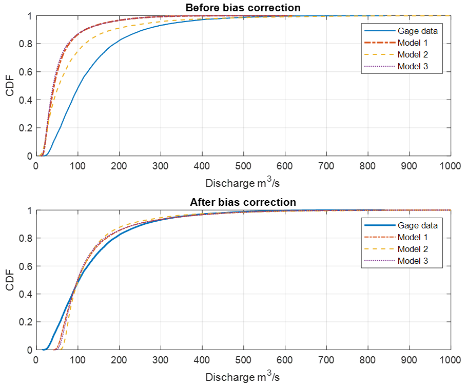
3.2. Bias Correction of the Climate Model Datasets

Global climate model datasets offer global time-series data sets. So initially, the data for our study area are extracted from the netCDF file of the global data series. The river discharge time series is extracted for the proposed site from the global data series. The predictions offered by the climate model datasets comprise of a lot biases, courtesy of the use of different grid structures and parameterization of the fluxes [44]. Without resolving the biases in the model, the accuracy of the result from that dataset will be compromised. As a measure of bias correction, different methods have been proposed that include linear regression, linear scaling [45], logistic regression, quantile mapping, empirical quantile mapping [46], distribution mapping [45], and a few others. This study chooses empirical quantile mapping method as the measure for bias correction because of its success in past research.

The eCDF (Empirical Cumulative Distribution Function) method categorizes the observed and modeled datasets for the same time period and develops a Q-Q map by plotting the sorted values against one another. Then, a transfer function is created by linear interpolation between the mapping points [47]. The empirical quantile mapping makes a comparison of empirical cumulative density function (eCDF) for the observed (gage station data set) and simulated river discharge for the historical time period [48]. The eCDF approach is based on the distribution mapping method with the fundamental premise to match the distribution of the observed dataset to the modeled historic dataset. The assumption of this approach is that for a given percentile; the adjustment function for the historical and future periods remains the same. The computational process can be mathematically expressed as

$$X_{fut.adjust}=X_{fut}+F_{obs}^{-1}\left(F_{mod}\left(X_{fut}\right)\right)-F_{mod}^{-1}\left(F_{mod}\left(X_{fut}\right)\right)$$

(1)

Here, $F_{obs}$ and $F_{mod}$ are the cumulative distribution function for the observed and modeled dataset of the historical time, respectively; $X_{fut}$ is the CDF equivalent of the $F_{mod}$ for the future time period, and $X_{fut.adjust}$ is bias-corrected output by eCDF method.

Figure 2 shows the differences in CDF curve for the GCMs and the observed historical data. The plot on the top is prior to the bias correction, while the bottom plot is after performing bias correction in the datasets. The differences in the modeled and observed values can be seen in the figure before bias correction, which proves the existence of biases in the modeled historical data, and so it is imperative to reduce them in order to obtain better-quality model data. The proposed method aims to minimize the differences in this curve and generate a relationship, and thus bias-corrected historical data are generated. This figure shows the CDF curve comparison for the corrected data with the observed data, which corroborates the minimization of biases.

3.3. Quantification of Future Design Flow

Bias-corrected future data give a hydrograph for the given time period. Flood management strategies and infrastructure are essentially built for extreme flood flows at different recurrence intervals. Depending on how the data sets are distributed, methods for the flood extreme data computation are selected.

Different distributions can be applied for this procedure depending on various parameters, including but not limited to flow time series data, climatic and environmental background, and geographical position. Studies have approached different distribution measures to determine the favorable distribution measure for calculating the flood frequency values at various return periods. For instance, Topaloglu [49] concluded the Gumbel method to be the best fit based on Chi-square test for the study area of Seyhan River basin; Abida and Ellouze [50] performed a best-fit analysis for Tunisia and found that generalized extreme values (GEV) were more suitable for North Tunisia, whereas for South Tunisia, it was the generalized logistic method (GLO). These examples suggested that the best-fit analysis depends on the study area under consideration and so this study performed best-fit analysis based on the Kolmogorov–Smirnov (K-S) test to determine the distribution system for determining the flood frequency and chose the GEV method. The GEV method is widely accepted measures for extreme value analysis [51]. GEV is a standard approach developed within extreme value theory, and the only limit distribution of properly normalized maxima of a sequence of independent and identically distributed random variables is the GEV distribution. For extreme value analysis, firstly, the distribution of the annual peak discharge needs to be identified. This research has different sets of annual peak discharges given the various models considered. In this regard, the author performed a distribution analysis to find the best-fit distribution for most of the datasets, which was found as the GEV method. GEV combines tree parameter models, namely Gumbel ($\xi$ = 0), Fréchet ($\xi$ > 0), and Weibull ($\xi$ < 0). In the past, different studies have adopted this measure for flood frequency analysis [52,53,54], and this study also uses this method to determine extreme floods. The equation for the GEV distribution for determining the yearly maximum is determined using the equation below:

$$\mathrm{GEV}\left(x:\mu ,\sigma ,\xi \right)=\left\{\begin{array}{c}\exp \left\{-{\left[1+\xi \left(\frac{x-\mu }{\sigma }\right)\right]}^{-\frac{1}{\xi }}\right\} if \xi \ne 0\\ \exp \{-\exp \left[-\left(\frac{x-\mu }{\sigma }\right)\right]\} if \xi =0\end{array}\right.$$

(2)

Here, $\mu ,\sigma , \mathrm{and} \xi$ are the parameters of $\mathrm{GEV}$ that represent the location, scale, and shape of the data. The GEV distribution essentially provides the flood extremes for different return periods. In this study, preference is given to 100 y and 500 y flood for comparison with historical values.

Furthermore, to apply the climate model data for the regional scale, downscaling of the dataset is required, and a commonly used method for this is the change factor methodology (CFM), also known as the perturbation or delta change method (DCM). Although studies have been conducted on the proper procedure for calculating future peak flow using CFM, clear guidelines for which steps to take for what parameters are still hazy [55]. The mathematical formulation of CFM includes additive and multiplicative approaches. The additive approach takes the arithmetic difference between the modeled historical and modeled future data sets and then adds the difference to the observed data set, in contrast to the multiplicative approach, which takes the ratio of future simulated values and historical simulated values and multiplies it with the observed historical values. The additive approach is expected to produce a better estimate for absolute change in any variable, while the multiplicative approach does so for the relative change in values of any variable [56]. Since the research aims to provide an insight on the relative change in flooding peaks over the years, this study opts for the multiplicative approach of the CFM.

For this approach, firstly, the ratio of future simulated peak flow and historical simulated peak flow is calculated, which is known as the delta change factor (DCF) [32]. This DCF value, when multiplied with the existing peak flow value, will yield the future peak flow values. Mathematically, it can be expressed with the relationship as follows:

$$\mathrm{DCF}= \mathsf{\Delta }Q=\frac{Q_{fut,mod}}{\begin{array}{c}{Q}_{hist,mod}\\ \end{array}}$$

(3)

where, $\mathsf{\Delta }Q$ = delta change factor for the peak discharge; $Q_{fut,mod}$ = modeled future peak discharge; $Q_{hist,mod}$ = modeled historical peak discharge

$$Q_{fut}=\mathrm{DCF}\times Q_{obs}$$

(4)

where $Q_{fut}$ = final future peak discharge, and $Q_{obs}$ = observed peak discharge.

DCF is calculated for every scenario and return period. A higher value of DCF is considered for this study, such that the maximum increase in flood data in the future could be used. The methodology framework that is used for the overall procedure of this study is illustrated by Figure 3.

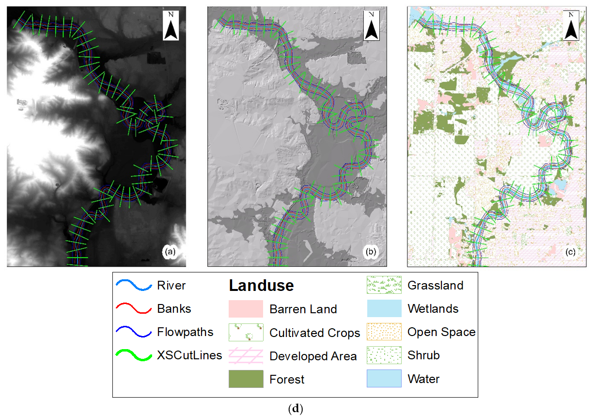
3.4. Inundation Modelling

The floodplain regime is obtained from the model in HEC-RAS. A certain section of the river is considered, i.e., in between two gage stations. The digital elevation model extracted from the geospatial gateway is converted into a tin file. The centerline of the river is marked in between two gage stations, i.e., upstream, and downstream gage stations. The bank lines are demarcated based on the existing satellite image of the area. The flow path lines are drawn, and the center, right, and left are defined for each line. The cross sections are generated across the river section at a certain level of distance with more at the meandering of the river. Then, the manning’s coefficient values are assigned to each cross section based on land use. Land use is extracted from government sites, i.e., Multi-Resolution Land Characteristics Consortium Viewer (MRLC Viewer). The assigned values of manning’s coefficient are given in

Table 2. Manning’s coefficient considered for the simulation.

Land Use	Allowable Manning’s Range	Assigned Manning’s
Developed Open Space	0.030–0.050	0.030
Developed Low Intensity	0.050–0.120	0.050
Developed Medium Intensity	0.060–0.140	0.060
Developed High Intensity	0.080–0.200	0.080
Undeveloped Barren Land	0.025–0.035	0.025
Undeveloped Grassland	0.025–0.050	0.025
Undeveloped Shrub/Scrub	0.070–0.160	0.070
Undeveloped Mixed Forest	0.100–0.160	0.100
Undeveloped Deciduous Forest	0.100–0.160	0.100
Undeveloped Evergreen Forest	0.100–0.160	0.100
Agricultural Cultivated Crops	0.025–0.050	0.025
Agricultural Pasture	0.025–0.050	0.025
Wetlands Forested	0.045–0.150	0.045
Wetlands Non-Forested	0.050–0.085	0.05

. The Manning’s coefficients considered for the simulation are different in the case of bank lines; however, for the centerline of the river, they are the same at each cross section, i.e., 0.03. The minimum value from the range of Manning’s coefficient is considered at the bank lines. The peak flow value is assigned, and steady flow analysis is computed. After the computation, the inundation area around the river can be observed. The inundation model is prepared for bias-corrected historical data and future projected data. The inundation maps were then prepared in Geographical Information System (GIS) by transferring the HEC-RAS files to the GIS format.

3.5. Comparison of Gage Height from USGS and HEC-RAS Model

For the downstream gage station, the gage height is extracted for different value of runoff in different years from USGS. These gage heights are the standard values obtained from the USGS. Then, the gage height for the same year of runoff data from CMIP6 model after the bias correction is obtained by inundation modelling for each value of peak runoff. Then, the comparison of the gage height obtained from runoff value of same year is compared and involves the calculation of Nash–Sutcliffe efficiency (NSE), root mean square (RMSE), percent bias (PBAIS), and standard deviation ratio (RSR). The calculation of these parameters helps in the calibration and validation of the model. Historical runoff value is considered for the calibration and future projected values are considered for the validation. To check the model’s calibration and validation, the values are NSE ≥ 0.65, PBIAS ≤ ±10%, and RSR ≤ 0.60 [57]. The formula involved in the calculation of values mentioned are presented in

Table 3. Mathematical interpretation involved in comparing observed and modeled gage height.

Indices/Parameters	Mathematical Representation
Nash–Sutcliffe Efficiency (NSE)	$1-[\frac{{{\displaystyle \sum }}_{i=1}^n{\left(R_{oi}-R_{ci}\right)}^2}{{{\displaystyle \sum }}_{i=1}^n{\left(R_{oi}-R_{o,mean}\right)}^2}$
Root mean square (RMSE)	$\sqrt{\frac{1}{n}{{\displaystyle \sum }}_{i=1}^n{\left(R_{oi}-R_{ci}\right)}^2}$
Percent bias (PBAIS)	$\frac{{{\displaystyle \sum }}_{i=1}^n\left(R_{oi}-R_{ci}\right) * 100}{{{\displaystyle \sum }}_{i=1}^n{R}_{oi}}$
Standard Deviation Ratio (RSR)	$\frac{RMSE}{Standard Deviation}$

. Mathematical interpretation is involved in comparing observed and modeled gage height. $R_{oi}$ and $R_{ci}$ represent the gage height from USGS and model, respectively, for the same date runoff value. The corresponding runoff is also from the USGS and CMIP6 models, respectively. $R_{o,mean}$ represents the mean value of n number of data considered for comparison.

3.6. Comparison of Floodplain Regimes with FEMA

FEMA prepares the hazard-prone area map for the response to the flood management and marks the most vulnerable area for the quick response. FEMA prepares the map considering the value of runoff for the particular year. Mostly, it considers the latest available runoff value. The inundation area obtained from the HEC-RAS is compared with the FEMA map by overlaying the two inundation extents in GIS. This is the scientific process for the validation. The similarity in inundation from the model and FEMA validates the model for the recent value of runoff. Moreover, validation confirms the inundation extent for the recent value of runoff from the model, and the future projected inundation extent can be considered from this study. So, the future inundation extent addresses the area under high risk of flood hazard and frequency.

3.7. Evaluation of Change in Inundation Extents

The change in flood inundation extent is directly obtained from the difference in flood plain in 100- or 500-year return period and flood plain during historical time. The value of flood is expressed in terms of percentage. The change can be governed by the mathematical relation shown in the equation below [58].

$$\mathsf{\Delta }\mathrm{IE} \left(\%\right)=\frac{I{E}_F-I{E}_H}{I{E}_H}\times 100$$

(5)

IE represents the change in inundation extent in percentage, $I{E}_F$ is the inundation extent in 1 in 100 years or 1 in 500 years for the future runoff, while $I{E}_H$ is the inundation extent from historical runoff value. The inundation extent is in square kilometers.

4. Results

This section presents the allegiance of the Global Climatic Models to propose the runoff value and to indicate the flood plain over Rock River area for the historical period. The runoff value for the modeling is evaluated and corrected using bias correction and compared with data from USGS station. Then, the simulated model is calibrated and validated. The computed flood plain regimes are also compared with the FEMA maps. So, the discussion is focused on (i) data computation, (ii) output from flood modeling, (iii) calibration and validation, and (iv) the evaluation of change in flood inundation extent.

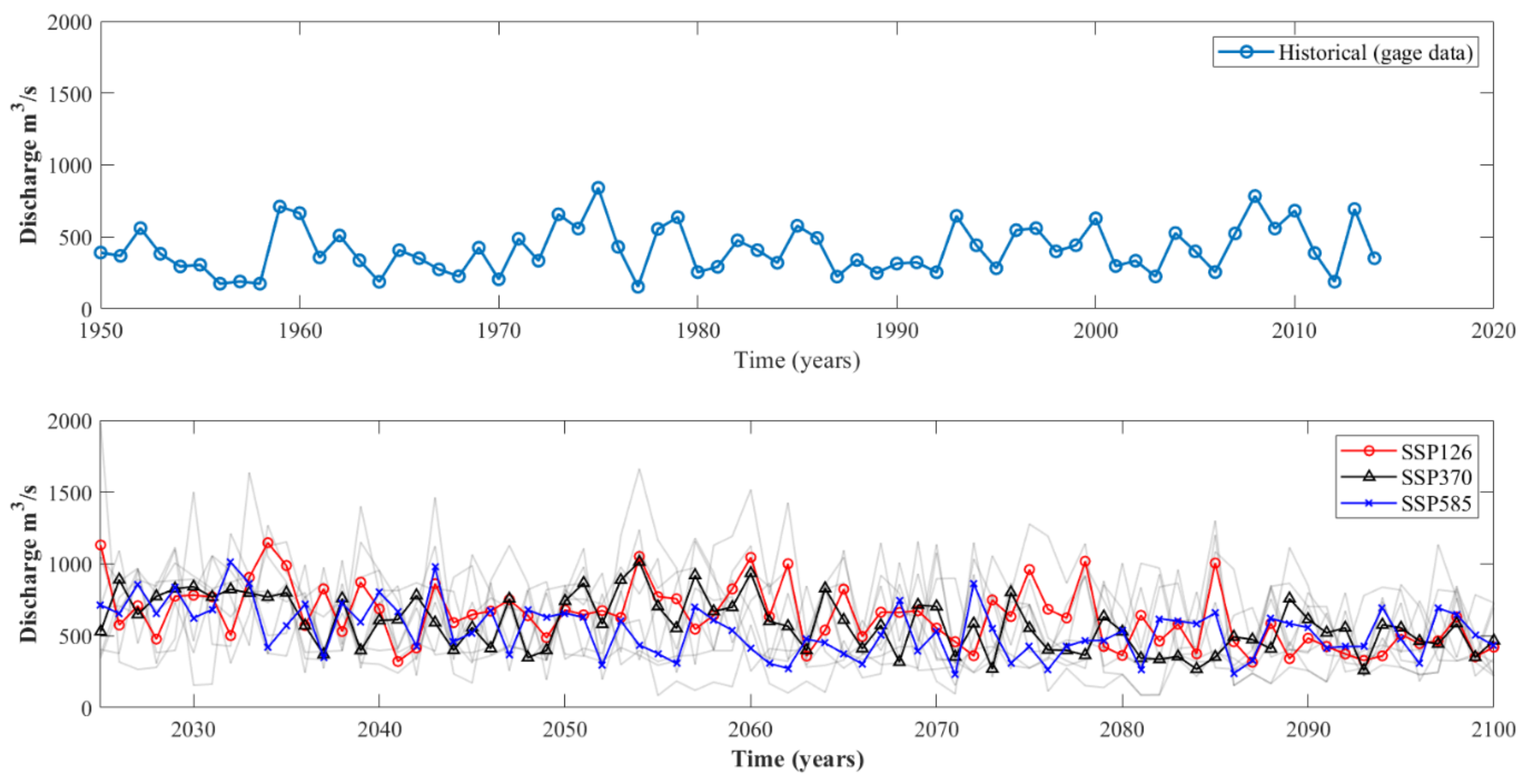
4.1. Generation of Future Projected Time Series Datasets from CMIP6

This study uses the gage station discharge data as the observed data set for the time- period ranging from 1950 AD to 2014 AD. This gage station data set served as an observed data for bias correcting the CMIP6 data set so that the uncertainty of the climate model could be handled, and biases could be minimized. Firstly, the observed value and the historical model value were bias-corrected, and the final values post-bias-correction were analyzed. Prior to the bias correction method, the significant difference in the CDF curve between the modeled and the observed values can be seen as depicted in Figure 4. Annual peak flow for historical (top) and future modeled (bottom) datasets. The bold lines in the future peak flow plot are the mean of ensemble model for each scenario, and three different markers represents the scenarios, as shown in the legend in the plot. Similarly, the figure also shows that the bias in terms of the CDF curve has been dealt with since the difference between the plots looks very small. Using the same transformation factor, the future flood values were determined for all the variant levels and the models, which comprise a total of 43 data points. Ensemble means of the modeled future data yielded the yearly hydrograph for the three scenarios (SSP126, SSP370, and SSP585). The goal of this research is to understand the risk of extreme river discharge, and so maximum annual flood is considered for the purpose of this study. Figure 4 (top) shows the yearly hydrograph that is obtained from the observed gage station data, and Figure 4 (bottom) shows the same for the future bias-corrected data for every model. The lighter shade of hydrograph in Figure 5 represents all the models and variants considered, while the darker lines are the final ensemble values in different scenarios. This represents the uncertainty that the climate model offers and thus corroborates that there is a need to minimize such uncertainties and biases in the model. This hydrograph shows an increase in annual peak discharge for the future projected data as compared to historical data, determining possible flooding escalation in the future. More extreme values are caused because of the lower-intensity scenario as opposed to the higher-intensity scenario.

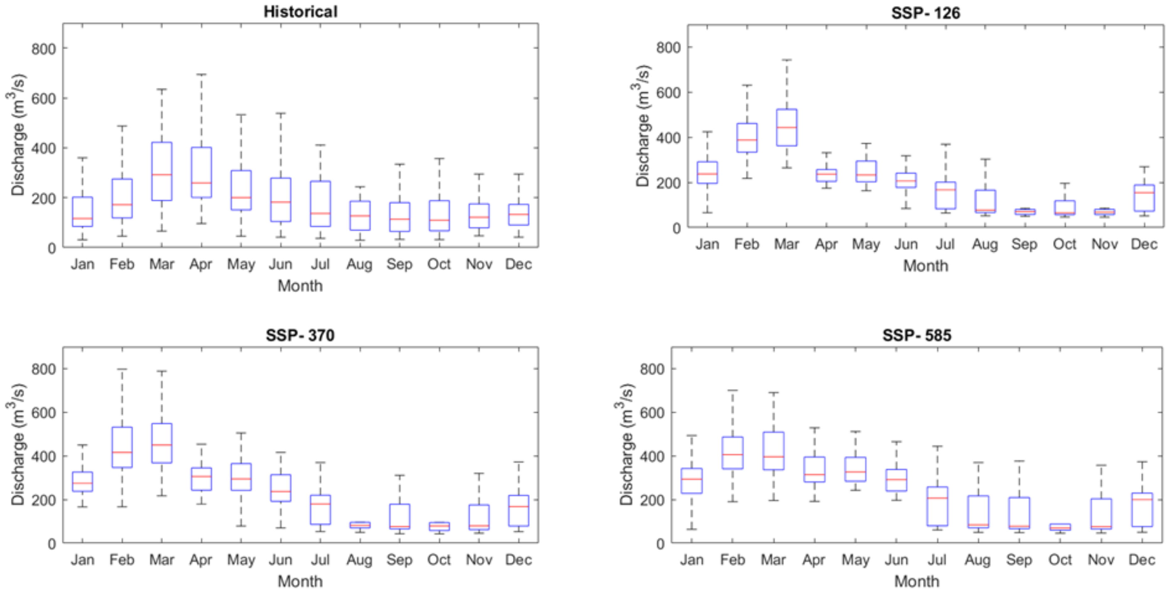
4.2. Change of Monthly Peak Discharge

This study mostly focused on the peak discharge projection which hides the flow pattern over the years and so monthly variation for the historical and future time-period is analyzed. Upon carefully analyzing the monthly discharge data, it can be visualized that both the minimum and maximum extreme values have increased in the future scenarios, especially in the months of January, February, and March. This result can be visualized in Figure 5. Monthly peak variation over the years is given for historical period and future projected scenario for three emission scenarios. However, in the month of April, though the historical data showed higher extreme values, the future model predicts lower value for the same. This foretells that climate change will alter the precipitation pattern, considering there is significant change in the monsoon season. The peak value of flow changed from the month of April in the historical time period to the months of February and March in the future time period. This suggests that not only will there be an increase in peak flow in some months, but that the month in which the peak flow occurs will also change in the future.

4.3. Determination of Future Flood Extremes for Different Return Period

Bias-corrected future annual discharge data are then used to calculate the design peak flows for different recurrence intervals, which includes 2 years, 5 years, 10 years, 50 years, 100 years, and 500 years, using the GEV (L-moments) approach. This method is implemented for gage station discharge data, historical modeled data, and bias-corrected future data. If it was not evident from the hydrograph, these discharge values at different exceedance levels corroborate the flooding increase in future scenario due to climate change. Using the return period discharge calculated using the GEV method for the gage, historical modeled, and future modeled data, DCF is calculated for each case of recurrence interval by dividing the future modeled data by historical modeled data. The value of DCF for each scenario and recurrence interval is tabulated in

Table 4. DCF values for values for different return period and scenarios.

Scenarios	2 y	5 y	10 y	25 y	50 y	100 y	500 y
SSP126	1.029	1.438	1.691	2.008	2.225	2.444	2.940
SSP370	0.980	1.291	1.473	1.684	1.828	1.964	2.250
SSP585	0.902	1.276	1.508	1.794	2.004	2.211	2.691

. According to this value, extreme floods are more severe in lower-intensity scenarios than in higher-intensity zones. This implies that the increase in GHG emission, land-use change, and other characteristics will increase the flooding extent, but the change in flood extent is not proportional to climate change. Extreme values are less in the higher scenario but high in the lower scenario, but in both instances, the future extreme value suggests an increase in flooding compared to that given by historical data. This necessitates the incorporation of climate change issues in strengthening the flood control measure for robust management planning strategies.

Taking the highest value of the DCF to incorporate a more conservative analysis to understand the flooding extent proposed by this scenario, we choose DCFs of 2.5 and 3.0 for 100-year and 500-year flood, respectively, to determine the peak future flood. Calculation yielded the peak future 100-year and 500-year flood to be 2273.42 m³/s and 3205.70 m³/s, respectively. Later in this research, a flood plain inundation map is constructed with these values to understand the implications if flooding of this extent occurs.

4.4. Comparison of Model Output with USGS

After the model is prepared in the HEC-RAS, we can determine the flood plain regime. Figure 6 shows river centerline, bank line, and delineated cross sections for the digital elevation model (DEM), terrain (TIN), and land use for the study area. The computed regime will give the extent of flooding around the selected river stretch. The runoff from the USGS station is considered, and gage height for each runoff is taken out from the model.

The gage height from the USGS station is also extracted for the similar runoff considered, and then, by a comparison of the observed and modeled runoff, i.e., $R_{oi}$ and $R_{ci}$ the model is calibrated and validated. The model is calibrated as NSE > 0.6, PBIAS < 10%, and RSR < 0.6. Additionally, the value of correlation obtained is 0.99. The model is validated as NSE > 0.8, PBIAS < 10%, and RSR < 0.6, and the correlation value is 0.96. The values computed are presented in

Table 5. Values for calibration and validation of model.

Model	RMSE	RSR	NSE	PBias	R2
Calibrated	0.270	0.384	0.853	7.192	0.999
Validated	0.091	0.358	0.872	−0.353	0.969

.

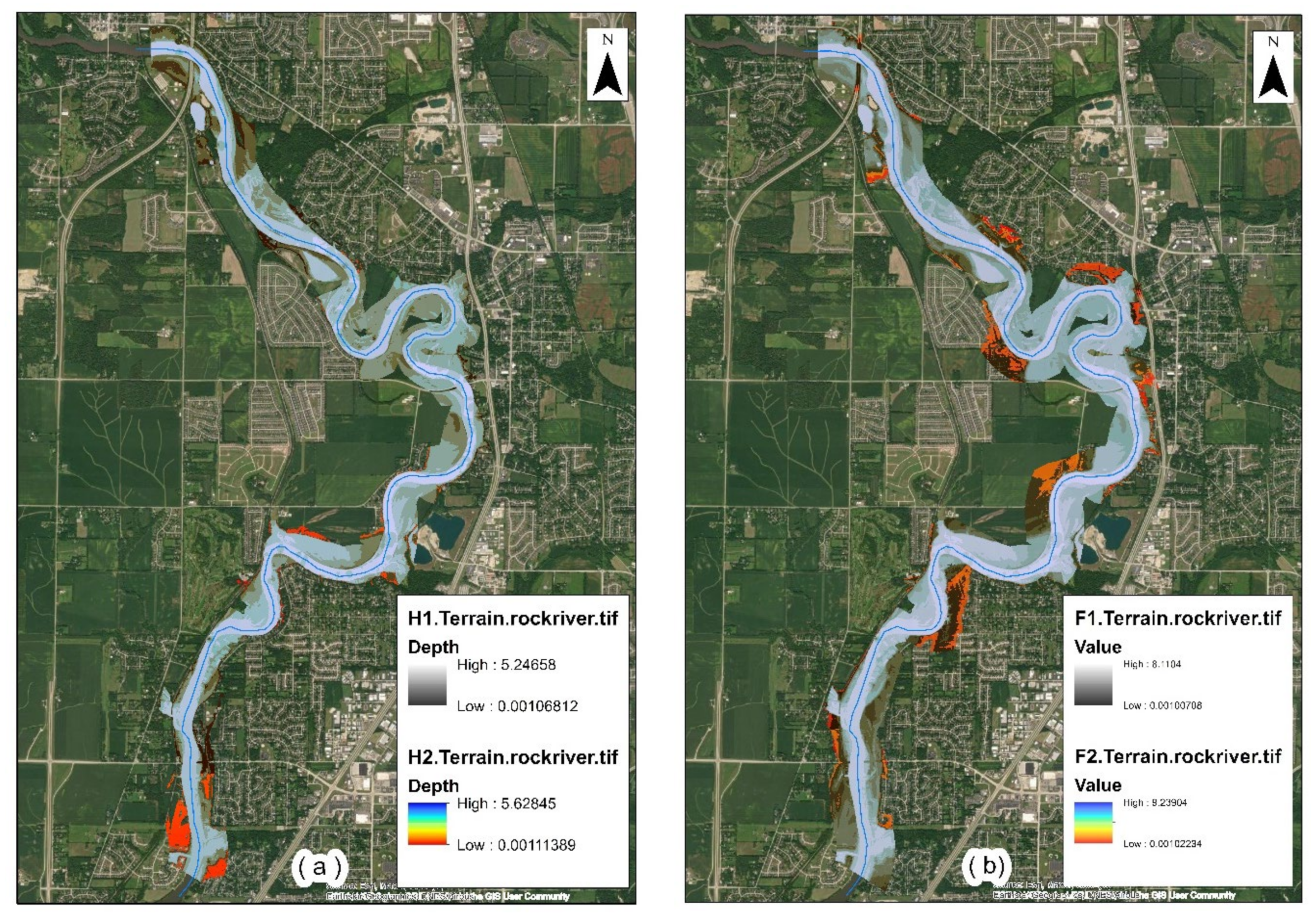
4.5. Representation of Model Output and Identification of Flood Prone Areas

The model then can be used to present the flood regime for the historical time and the future projected values. The flood regime obtained is for 100-year and 500-year frequency. The historical runoff values for 100 y and 500 y return period is 909.37 m³/s and 1068.57 m³/s. The increase in flood depth can be seen in the map in Figure 7. The future projected values for 100-year and 500-year return period are 2273.43 m³/s and 3205.701 m³/s. The flood depth can be seen in the map in Figure 8. From the maps, there is greater inundation extent in future projected values for 100-year and 500-year return flood. This gives the impact of climatic models that is affecting the runoff as well as the inundation extent. The map clearly shows the increase in inundation extent. The inundation area of 100-year return for 909.37 m³/s and 2273.425 m³/s is 7,517,275 m² and 9,044,828 m², respectively. The inundation area of 500-year return period for 1068.567 m³/s and 3205.701 m³/s is 78, 34,389 m² and 10,228,351 m², respectively. Certainly, the area in map also signifies the clear increasing impact in runoff by considering several climatic change factors from CMIP6. So, the flood-prone area exposes widely due to climate change; however, considering several scenarios from GCM, flood risk continues to increase due to the change in the high degree of socio-economic development. So, the research work clearly depicts the flood hazard area for the future projected values.

The land use that was affected by the 500-year return period flood is also computed. Thus, the hazard-prone zone covers 1.49 km² of developed low-intensity land, 0.43 of developed medium-intensity land, 0.059 km of developed high-density land, 1.8 km of cultivated land, 1.22 km of forest, and 1 km of open space and barren land. So, 1.49 km of the developed area with low intensity is affected, which means that this area is prone to future expansion. The comparison of the existing land use affected by the runoff values for 100 y and 500 y return period is given in the table below.

Table 6. Table showing percentage of land use affected in different return period.

Grid Code	Type	Percentage of Land Use Affected
		100 y (Historical)	500 y (Historical)	100 y (Future)	500 y (Future)
11	Water	0.31	0.30	0.30	0.23
21	Open Space	0.07	0.07	0.07	0.10
22	Developed Low Intensity	0.07	0.08	0.08	0.16
23	Developed Medium Intensity	0.03	0.03	0.03	0.05
24	Developed High Intensity	0.01	0.01	0.01	0.01
41	Forest	0.14	0.14	0.14	0.13
71	Grassland	0.03	0.03	0.03	0.03
81	Pastureland	0.02	0.02	0.02	0.02
82	Cultivated Crops	0.20	0.21	0.21	0.19
90	Wetlands	0.10	0.10	0.10	0.08
95	Herbaceous Wetlands	0.01	0.01	0.01	0.01

shows the gradual increase in hazard-prone area in the medium-density developed area. So, in reference to this research study, the medium-density developed area cannot be considered under the future urban expansion zone. In the 500-year return period, projected flood resembled the specific change in hazard prone area of medium-density developed land use type, i.e., from 0.3% to 0.5%.

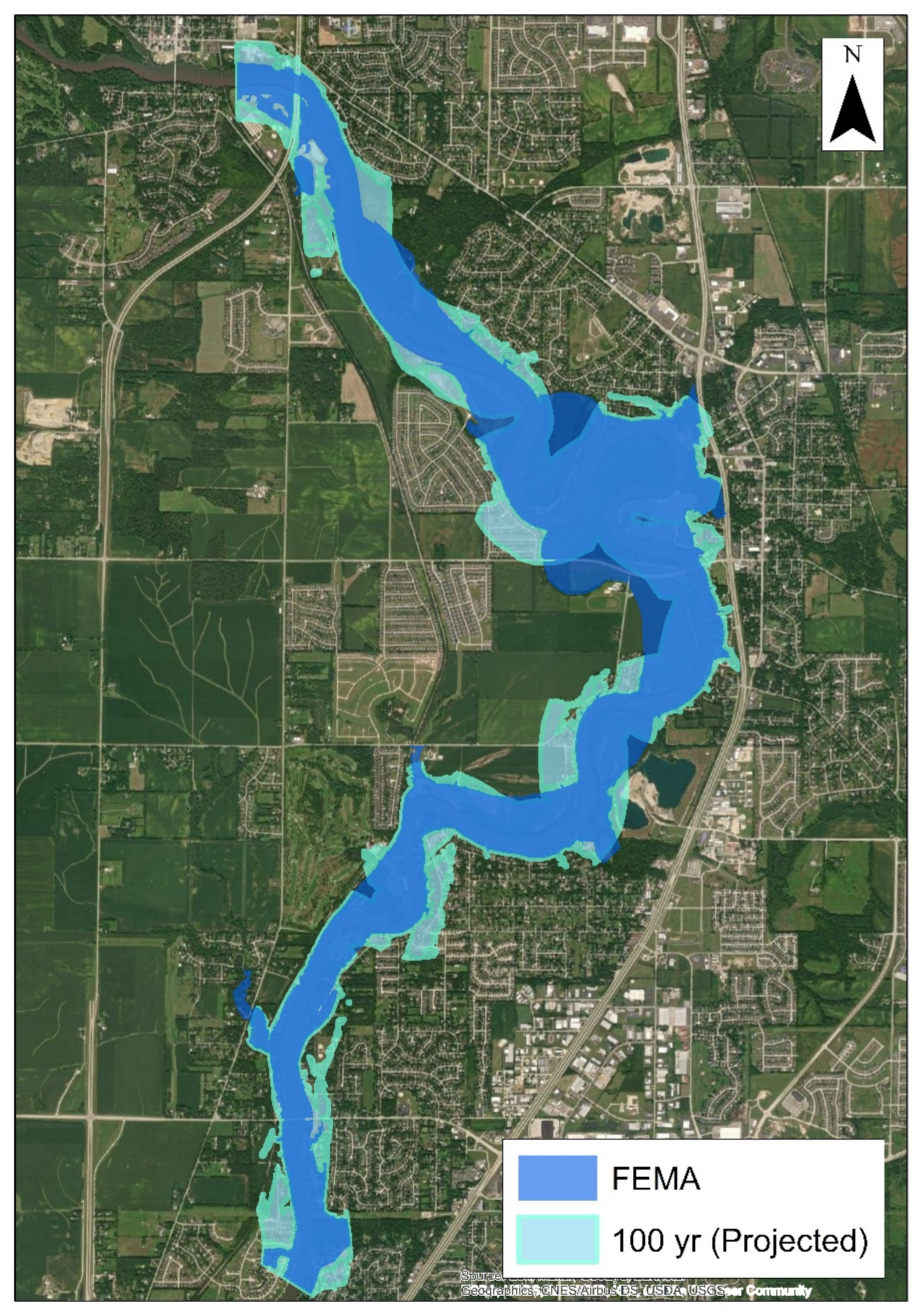
4.6. Comparison with FEMA Map

To understand the severity of the increasing flood for both 100-year and 500-year projected values, the map by FEMA is compared with the projected value of the 100-year return period. The inundation map created from the HEC-RAS model is compared with FEMA Map. The HUCODES are given in FEMA, which not only indicates the prone area but also the effective date through which the FEMA maps are valid. The HUCODES for the watershed of the stretch of the river selected for this study are given as follows: 17201C0129E, 17201C0133E, 17201C0141E, 17201C0142E, 17201C0144E, 17201C0143E, and 17201C0256E. The FEMA map effective for this site is dated 17 February 2016, and the runoff considered is the 100-year return period. The comparison of the FEMA map with the 100-year return period flood, as shown in Figure 8, shows that the inundation extent is high for the projected value. The comparison shows the most vulnerable areas around Rock River. As FEMA prepares a quick response plan based on its flood analysis, the comparison shows the more vulnerable area for the future predicted values considering several climatic models, which suggests the need for incorporating the climate change factor for decision making in flood plain management strategies.

4.7. Quantification of Inundation Extents

Table 7. Percentage change in inundation extend.

Return Period	$\mathit{I}{\mathit{E}}_{\mathit{F}}\left({\mathbf{km}}^2\right)$	$\mathit{I}{\mathit{E}}_{\mathit{H}}\left({\mathbf{km}}^2\right)$	IE%
100 y	9.045	7.517	20.321
500 y	10.228	7.834	30.557

shows the change in inundation extent for 100-year and 500-year flood events for all the climatic scenarios considered. The change is quantified by considering the historical and projected future values. This change in flood inundation extent is with respect to the historical flood regimes, which is calculated by considering the area of inundation extent in square kilometers. The change in both 100 y and 500 y flood event inundation extent is greater than 20%. This emphasizes that the river is on the verge of a flood-prone zone, i.e., the probability of severe flooding in the high-runoff time period [58]. This also indicates that the probability of damage by flood in the future increases. So, this research could be helpful for county planners regarding the urban zoning of the area around this stretch by implementing quantitative options for land use to support making quick response action against imminent destruction.

5. Discussion

The uncertainty in the river is due to its rise from normal flow depth, which has been affecting human settlement areas. The anthropogenic activities are causing the narrowing of the river and the expansion of settlement areas. Human civilization growth has always started from the banks of rivers or, more specifically, from coastal areas due to easy access to basic resources, e.g., water. After the Black Hawk War, in 1833, the settlement around Rock River of people of Kentucky and Tennessee evidence that the site considered in this research work has seen increasing numbers of settlement areas since antiquity [59]. The increase in civilization has resulted in urbanization and industrialization, causing changes in climate that have affected flooding in several parts of the world. In the spring of 2002, Illinois State received maximum flooding due to escalated rainfall intensity in a short period of time. For about 9 days, the flood stage of Rock River escalated [60]. Then, the flood impact around Rock River increased due to several climatic factors. So, the research study considers the CIMIP6 climate model with different socio-economic scenarios to present the flood impact for future projection.

5.1. Future Projection of Discharge Data Based on CMIP6 Model

The CMIP6 climate model dataset after bias correction and downscaling shows increases in the flood flow regime in the future (2025–2100) as compared to the historical period (1950–2014). In the case of both annual peak discharge as well as monthly peak discharge, increases in the values were observed. This result agrees with past research, which includes flood change analysis based on precipitation and temperature data sets. For the annual peak flow, Xiang et al. [45] found an increasing trend for the near future and a slight decreasing trend in the far future, which is consistent with our result, where we can see a decreasing trend in the far future. This suggests that the extremity will be more serious in the near future than in the far future context. Adib and Harun [61] determined a decrease in streamflow for the months of April and May because of high temperature in these seasons in the case of Malaysia, with worsening condition for the SSP-585 scenario. This made us believe that temperature and precipitation patterns need to be analyzed to understand the change in flow pattern in the given study area. In addition, a proper and detailed understanding of climate models and all the parameters they consider in developing datasets will also come in handy to interpret the change in hydrological regime from historical to future context. Additionally, the increase in monthly peak for some months and change in the month in which the peak occurs agrees with the results of Xiang et al. [45], who found a change in peak month from the month of August to July. In most past research studies, the largest change in flow values has been due to the higher emission scenario, but this study had a different outcome, which suggested higher values for the lower emission scenario [62]. This means that the likelihood of higher flooding is due to the SSP-126 emission scenario as opposed to the SSP-585 emission scenario. The current study provides new insights into the relation of the emission scenario and flow values. In most past studies, just through the graphical representation is the increase in streamflow denoted by the increase in emission scenario and streamflow [63]. However, the losses according to the location of the watershed are not considered. The loss is high in high-elevation subbasins, as they are sensitive to temperature, evapotranspiration, precipitation, and albedo changes, which have a significant effect on downstream watersheds [64]. The watershed of Rock River is in Wisconsin, which is a low-elevation area, and at certain high-emission scenarios due to low losses, the stream flow value is high. These reasons are in consensus with current findings [65].

Even though, with a much higher emission scenario, the peak flow decreases more than that of the low-emission scenario, comparing these peaks with the current pattern, it suggests more flooding in the future regardless of the emission scenarios. Thus, this increased flow and high unpredictability of future floods will substantially affect the hydrological and ecological processes of the watershed, thereby making the system more vulnerable to flood events.

5.2. Flood Innundatation Mapping Analysis Using HEC-RAS Model

After the finalized data for historical and future flood values, the model is prepared in HEC-RAS. The model prepared in HEC-RAS is calibrated considering the historical values and validated considering the recent flow values. The calibration and validation are based on gage height obtained from each considered flow datum. The calibration and validation are performed by calculating and comparing the values of RMSE, RSR, NSE, PBias, and R². After this process, the model is used to obtain the flood extent for future projected flow values of return periods of 100 years and 500 years. The flood extent from HEC-RAS is presented in a map using GIS. The flood extent shows that the greater portion of the developed low intensity is affected. The land use affected is determined by intersecting the shapefiles of land use and flood extent in GIS. The urban planning concept starts from the development of low intensities areas, so the research study suggests the proper planning of these areas is needed for future urban expansion. To achieve sustainable urban development, by digital data integration and simulation, the planners start the zoning of any area. So, to the planners and decision makers, the resulting information must provide vulnerable areas to urbanize and revise the urban expansion zone [66]. So, this is suggested by the flow values obtained from considering the climate change models (CMIP6).

Furthermore, to show the hazard prone zone areas, flood extent is also compared with the map prepared by FEMA and for the mathematical representation of flood-prone zone change in inundation extent is calculated in terms of percentage. The inundation extent from the prepared model is overlaid with the FEMA inundation extent. From just overlaying, it can be seen on the map presented that some portions of the flood extent have crossed the FEMA’s map. So, the inundation map developed in the research study might be helpful to prepare a quick response plan for the areas. Additionally, after the quantification of the inundation extent, the incremental inundation extent is 20% and 30% with respect to historical data. This reflects that the inundation zone, i.e., hazardous zone, is increasing in both 100-year and 500-year return periods. So, proper planning is required in these areas as they are flood-prone zones, i.e., there is high probability of severe flood in high run-off time period [58]. So, the stretch of the river considered for this research is in a high flood-risk zone, which is emphasized by comparison with the FEMA map and the quantification of inundation extent. The research can be helpful for the planning of urban expansion area along the stretch of river considered in this research study, as the flow value considered is corrected from climatic models with varying scenarios due to climate change, i.e., the future projected flow value is obtained by considering climate change scenarios. According to an article accorded by the National Resource Defense Council in October of 2017, the flood maps prepared by the FEMA are inadequate for making response plans, as climate change factors are altering rapidly. Additionally, the inspector general of the NRDC in 2017 reported that the 58% of FEMA flood maps are outdated and do not consider climate change models during the projection of flooding [67]. In this regard, the authors presented the use of climate change in presenting the flood maps with the projected value where the climate model is considered. So, the extent developed from such projected value can be taken into consideration for future management planning. Since FEMA updates the flood maps every 5 years, the model used might be helpful for the prediction of future floods for similar kinds of rivers, as the author considered the location with more meandering too.

5.3. Uncertainities and Limitations

The study evaluates the historical simulation and future projection of discharge under climatic variations by sole application of river discharge datasets. For the future flood estimations, the uncertainties are due to GCMs, downscaling methodology, bias correction measures, emission scenarios, and hydrological models [68]. The river discharge dataset is used from only three models based on availability, and only three emission scenarios are considered. Future studies could evaluate based on other hydrological parameters such as precipitation, temperature, and wind speed and additional emission scenarios to explore in depth the impact of climatic factors on hydrological parameters. Various modeling modules can be considered for rainfall–runoff evaluation, and the usage of futuristic precipitation data can be applied for peak flow extrapolation. The bias correction method used in this study is a statistical measure that prioritizes the improvement of GCM output relationship with the observations, in turn ignoring the physical mechanism [69]. A further challenge with bias correction is the availability of daily streamflow data for the given timeline. Fortunately, this problem is not encountered in this study, although previous research has demonstrated the validity of applying a machine learning technique to interpolate missing data [70]. Additionally, bias correction was performed for river discharge strictly based on its historical datasets, which invites future studies to incorporate other hydrological parameters. Hydrological parameters such as groundwater flow, surface water flow, evapotranspiration, interception, infiltration, and change in soil moisture may change regularly due to regular changes in perviousness and imperviousness in the watershed area. The detailed study of such parameters requires a greater level of expert study in each field, and so that is not in the scope of our study. Furthermore, for bias correction and downscaling of the dataset, many more methods can be employed to deal with complex topographic features, unpredictable hydrological variations, and biases in climate model datasets. Past research has explored other procedures in terms of the forecasting of hydrological parameters such as Gravity Recovery and Climate Experiment (GRACE) [71], machine learning algorithms [72,73], and Internet of Things (IoT) [74,75]. A comparison of these measures with the CMIP6 model could be performed for further validation of the climate model and betterment in the forecasting study.

6. Conclusions

Climate change has caused significant changes in global hydrological patterns, ultimately leading to unexpected flooding or drought in the far future context. This research work inferred the implication of climate change at watershed of Rock River by modeling future projected flooding using the CMIP6 model and making a comparative study of flood inundation extent with the FEMA 100-year flood in terms of flood inundation map and then performing inundation analysis. The conclusion from this research is enlisted as follows:

• Due to climate change, there will be an increase in flooding situation in the future, with 100-year flood extent being 2.5 times the observed 100-year flood, while for the 500-year flood, the increase was 3 times the observed value.
• Three different scenarios (low, medium, and high) are considered for this study, and the results yielded suggest that as the scenario increases or becomes more extreme in terms of carbon emission, the extent of flooding severity decreases.
• Calibrated and validated HEC-RAS models showed similar inundation mapping for 100-year flood as the FEMA map, hence further authenticating the model.
• From the inundation analysis, the effect on land use by future and historical data is assessed, and as per this study, developed low-intensity land use seems to be complex in this study.
• As per the inundation area analysis, the future projected 100-year flood yielded more spatial coverage than the FEMA flood map, which invites the need to improve flood mitigation measures to handle the uncertainties proposed by climate change.
• The inundation extents for both 100-year and 500-year flood exceeded the value of 20%, which makes the river reach of this basin a flood-prone area when considering the future projected data. This suggests that though the watershed does not display much flood risk in the present scenario, the climate change factor uncovers the future possible risk for this basin.

The contribution of this research is to instill the necessity of climate change factor for flood extent analysis. The HEC-RAS model used in this project can be utilized for computing the inundation flood mapping for different scenarios in a given site. The framework applied in the research study of the watershed of Rock River, significant meanderings in the downstream, for flood forecasting can be used for other research as per the requirements. The result and analysis of this research still leaves many questions unanswered, and further analysis of CMIP6 model and understanding the why and how of the model could elucidate the reason behind the flood regime variation due to climate change. Additionally, future research could focus on the analysis of the underlying parameters’ contribution to river discharge, such as precipitation, temperature and wind speed, which could help explain the profile of change in river discharge due to climate change. Furthermore, attention could be directed to the statistical analysis of CMIP6 model data to yield more accurate data sets with less biases so that the efficiency of the model can be bolstered.

References

- Plantico, M.S.; Karl, T.R.; Kukla, G.; Gavin, J. Is Recent Climate Change across the United States Related to Rising Levels of Anthropogenic Greenhouse Gases? J. Geophys. Res. 1990, 95, 16617. [Google Scholar] [CrossRef]
- Ruddiman, W.F. The Anthropogenic Greenhouse Era Began Thousands of Years Ago. Clim. Chang. 2003, 61, 261–293. [Google Scholar] [CrossRef]
- Hodgkins, G.A.; Whitfield, P.H.; Burn, D.H.; Hannaford, J.; Renard, B.; Stahl, K.; Fleig, A.K.; Madsen, H.; Mediero, L.; Korhonen, J.; et al. Climate-Driven Variability in the Occurrence of Major Floods across North America and Europe. J. Hydrol. 2017, 552, 704–717. [Google Scholar] [CrossRef] [Green Version]
- Krajewski, A.; Sikorska-Senoner, A.E.; Hejduk, L.; Banasik, K. An Attempt to Decompose the Impact of Land Use and Climate Change on Annual Runoff in a Small Agricultural Catchment. Water Resour. Manag. 2021, 35, 881–896. [Google Scholar] [CrossRef]
- Kuttippurath, J.; Murasingh, S.; Stott, P.A.; Sarojini, B.B.; Jha, M.K.; Kumar, P.; Nair, P.J.; Varikoden, H.; Raj, S.; Francis, P.A.; et al. Observed Rainfall Changes in the Past Century (1901–2019) over the Wettest Place on Earth. Environ. Res. Lett. 2021, 16, 024018. [Google Scholar] [CrossRef]
- Horton, B.P.; Shennan, I.; Bradley, S.L.; Cahill, N.; Kirwan, M.; Kopp, R.E.; Shaw, T.A. Predicting Marsh Vulnerability to Sea-Level Rise Using Holocene Relative Sea-Level Data. Nat. Commun. 2018, 9, 2687. [Google Scholar] [CrossRef]
- Yin, J.; Yu, D.; Yin, Z.; Wang, J.; Xu, S. Modelling the Combined Impacts of Sea-Level Rise and Land Subsidence on Storm Tides Induced Flooding of the Huangpu River in Shanghai, China. Clim. Chang. 2013, 119, 919–932. [Google Scholar] [CrossRef]
- Wdowinski, S.; Bray, R.; Kirtman, B.P.; Wu, Z. Increasing Flooding Hazard in Coastal Communities Due to Rising Sea Level: Case Study of Miami Beach, Florida. Ocean. Coast. Manag. 2016, 126, 1–8. [Google Scholar] [CrossRef]
- Booij, M.J. Impact of Climate Change on River Flooding Assessed with Different Spatial Model Resolutions. J. Hydrol. 2005, 303, 176–198. [Google Scholar] [CrossRef]
- Marengo, J.A.; Espinoza, J.C. Extreme Seasonal Droughts and Floods in Amazonia: Causes, Trends and Impacts: Extremes in Amazonia. Int. J. Climatol. 2016, 36, 1033–1050. [Google Scholar] [CrossRef]
- Jenkins, K.; Surminski, S.; Hall, J.; Crick, F. Assessing Surface Water Flood Risk and Management Strategies under Future Climate Change: Insights from an Agent-Based Model. Sci. Total Environ. 2017, 595, 159–168. [Google Scholar] [CrossRef]
- Dankers, R.; Feyen, L. Climate Change Impact on Flood Hazard in Europe: An Assessment Based on High-Resolution Climate Simulations. J. Geophys. Res. 2008, 113, D19105. [Google Scholar] [CrossRef]
- Eyring, V.; Bony, S.; Meehl, G.A.; Senior, C.A.; Stevens, B.; Stouffer, R.J.; Taylor, K.E. Overview of the Coupled Model Intercomparison Project Phase 6 (CMIP6) Experimental Design and Organization. Geosci. Model Dev. 2016, 9, 1937–1958. [Google Scholar] [CrossRef] [Green Version]
- Furrer, R.; Sain, S.R.; Nychka, D.; Meehl, G.A. Multivariate Bayesian Analysis of Atmosphere–Ocean General Circulation Models. Environ. Ecol. Stat. 2007, 14, 249–266. [Google Scholar] [CrossRef]
- Maher, P.; Gerber, E.P.; Medeiros, B.; Merlis, T.M.; Sherwood, S.; Sheshadri, A.; Sobel, A.H.; Vallis, G.K.; Voigt, A.; Zurita-Gotor, P. Model Hierarchies for Understanding Atmospheric Circulation. Rev. Geophys. 2019, 57, 250–280. [Google Scholar] [CrossRef] [Green Version]
- Meehl, G.A. Global Coupled General Circulation Models. Bull. Am. Meteorol. Soc. 1995, 76, 951–957. [Google Scholar] [CrossRef] [Green Version]
- Annan, J.D.; Hargreaves, J.C. Understanding the CMIP3 Multimodel Ensemble. J. Clim. 2011, 24, 4529–4538. [Google Scholar] [CrossRef]
- Meehl, G.A.; Covey, C.; Delworth, T.; Latif, M.; McAvaney, B.; Mitchell, J.F.B.; Stouffer, R.J.; Taylor, K.E. THE WCRP CMIP3 Multimodel Dataset: A New Era in Climate Change Research. Bull. Am. Meteorol. Soc. 2007, 88, 1383–1394. [Google Scholar] [CrossRef] [Green Version]
- Knutti, R.; Sedláček, J. Robustness and Uncertainties in the New CMIP5 Climate Model Projections. Nat. Clim. Chang. 2013, 3, 369–373. [Google Scholar] [CrossRef]
- Lee, J.-Y.; Wang, B. Future Change of Global Monsoon in the CMIP5. Clim. Dyn. 2014, 42, 101–119. [Google Scholar] [CrossRef] [Green Version]
- Taylor, K.E.; Stouffer, R.J.; Meehl, G.A. An Overview of CMIP5 and the Experiment Design. Bull. Am. Meteorol. Soc. 2012, 93, 485–498. [Google Scholar] [CrossRef] [Green Version]
- Tan, M.L.; Ibrahim, A.L.; Yusop, Z.; Chua, V.P.; Chan, N.W. Climate Change Impacts under CMIP5 RCP Scenarios on Water Resources of the Kelantan River Basin, Malaysia. Atmos. Res. 2017, 189, 1–10. [Google Scholar] [CrossRef]
- Van Vuuren, D.P.; Edmonds, J.; Kainuma, M.; Riahi, K.; Thomson, A.; Hibbard, K.; Hurtt, G.C.; Kram, T.; Krey, V.; Lamarque, J.-F.; et al. The Representative Concentration Pathways: An Overview. Clim. Chang. 2011, 109, 5–31. [Google Scholar] [CrossRef]
- Sun, G.; Peng, F. Evaluation of Future Runoff Variations in the North–South Transect of Eastern China: Effects of CMIP5 Models Outputs Uncertainty. J. Water Clim. Chang. 2020, 11, 1355–1369. [Google Scholar] [CrossRef]
- Wuebbles, D.; Meehl, G.; Hayhoe, K.; Karl, T.R.; Kunkel, K.; Santer, B.; Wehner, M.; Colle, B.; Fischer, E.M.; Fu, R.; et al. CMIP5 Climate Model Analyses: Climate Extremes in the United States. Bull. Am. Meteor. Soc. 2014, 95, 571–583. [Google Scholar] [CrossRef] [Green Version]
- Zheng, H.; Chiew, F.H.S.; Charles, S.; Podger, G. Future Climate and Runoff Projections across South Asia from CMIP5 Global Climate Models and Hydrological Modelling. J. Hydrol. Reg. Stud. 2018, 18, 92–109. [Google Scholar] [CrossRef]
- Maghsood, F.F.; Moradi, H.; Massah Bavani, A.R.; Panahi, M.; Berndtsson, R.; Hashemi, H. Climate Change Impact on Flood Frequency and Source Area in Northern Iran under CMIP5 Scenarios. Water 2019, 11, 273. [Google Scholar] [CrossRef] [Green Version]
- Homsi, R.; Shiru, M.S.; Shahid, S.; Ismail, T.; Harun, S.B.; Al-Ansari, N.; Chau, K.-W.; Yaseen, Z.M. Precipitation Projection Using a CMIP5 GCM Ensemble Model: A Regional Investigation of Syria. Eng. Appl. Comput. Fluid Mech. 2020, 14, 90–106. [Google Scholar] [CrossRef]
- Moss, R.H.; Edmonds, J.A.; Hibbard, K.A.; Manning, M.R.; Rose, S.K.; van Vuuren, D.P.; Carter, T.R.; Emori, S.; Kainuma, M.; Kram, T.; et al. The next Generation of Scenarios for Climate Change Research and Assessment. Nature 2010, 463, 747–756. [Google Scholar] [CrossRef] [PubMed]
- O’Neill, B.C.; Tebaldi, C.; van Vuuren, D.P.; Eyring, V.; Friedlingstein, P.; Hurtt, G.; Knutti, R.; Kriegler, E.; Lamarque, J.-F.; Lowe, J.; et al. The Scenario Model Intercomparison Project (ScenarioMIP) for CMIP6. Geosci. Model Dev. 2016, 9, 3461–3482. [Google Scholar] [CrossRef] [Green Version]
- Chen, Z.; Zhou, T.; Zhang, L.; Chen, X.; Zhang, W.; Jiang, J. Global Land Monsoon Precipitation Changes in CMIP6 Projections. Geophys. Res. Lett. 2020, 47, e2019GL086902. [Google Scholar] [CrossRef]
- Navarro-Racines, C.; Tarapues, J.; Thornton, P.; Jarvis, A.; Ramirez-Villegas, J. High-Resolution and Bias-Corrected CMIP5 Projections for Climate Change Impact Assessments. Sci. Data 2020, 7, 7. [Google Scholar] [CrossRef] [Green Version]
- Shafeeque, M.; Luo, Y. A Multi-Perspective Approach for Selecting CMIP6 Scenarios to Project Climate Change Impacts on Glacio-Hydrology with a Case Study in Upper Indus River Basin. J. Hydrol. 2021, 599, 126466. [Google Scholar] [CrossRef]
- Ukkola, A.M.; De Kauwe, M.G.; Roderick, M.L.; Abramowitz, G.; Pitman, A.J. Robust Future Changes in Meteorological Drought in CMIP6 Projections Despite Uncertainty in Precipitation. Geophys. Res. Lett. 2020, 47, e2020GL087820. [Google Scholar] [CrossRef]
- Hamed, M.M.; Nashwan, M.S.; Shahid, S.; Ismail, T.B.; Wang, X.; Dewan, A.; Asaduzzaman, M. Inconsistency in Historical Simulations and Future Projections of Temperature and Rainfall: A Comparison of CMIP5 and CMIP6 Models over Southeast Asia. Atmos. Res. 2022, 265, 105927. [Google Scholar] [CrossRef]
- Try, S.; Tanaka, S.; Tanaka, K.; Sayama, T.; Khujanazarov, T.; Oeurng, C. Comparison of CMIP5 and CMIP6 GCM Performance for Flood Projections in the Mekong River Basin. J. Hydrol. Reg. Stud. 2022, 40, 101035. [Google Scholar] [CrossRef]
- Zamani, Y.; Hashemi Monfared, S.A.; Azhdari Moghaddam, M.; Hamidianpour, M. A Comparison of CMIP6 and CMIP5 Projections for Precipitation to Observational Data: The Case of Northeastern Iran. Theor. Appl. Climatol. 2020, 142, 1613–1623. [Google Scholar] [CrossRef]
- Namara, W.G.; Damisse, T.A.; Tufa, F.G. Application of HEC-RAS and HEC-GeoRAS Model for Flood Inundation Mapping, the Case of Awash Bello Flood Plain, Upper Awash River Basin, Oromiya Regional State, Ethiopia. Model. Earth Syst. Environ. 2022, 8, 1449–1460. [Google Scholar] [CrossRef]
- Patel, D.P.; Ramirez, J.A.; Srivastava, P.K.; Bray, M.; Han, D. Assessment of Flood Inundation Mapping of Surat City by Coupled 1D/2D Hydrodynamic Modeling: A Case Application of the New HEC-RAS 5. Nat. Hazards. 2017, 89, 93–130. [Google Scholar] [CrossRef]
- Farooq, M.; Shafique, M.; Khattak, M.S. Flood Hazard Assessment and Mapping of River Swat Using HEC-RAS 2D Model and High-Resolution 12-m TanDEM-X DEM (WorldDEM). Nat. Hazards. 2019, 97, 477–492. [Google Scholar] [CrossRef]
- El Bilali, A.; Taleb, A.; Boutahri, I. Application of HEC-RAS and HEC-LifeSim Models for Flood Risk Assessment. J. Appl. Water Eng. Res. 2021, 9, 336–351. [Google Scholar] [CrossRef]
- Bertalan, L.; Rodrigo-Comino, J.; Surian, N.; Šulc Michalková, M.; Kovács, Z.; Szabó, S.; Szabó, G.; Hooke, J. Detailed Assessment of Spatial and Temporal Variations in River Channel Changes and Meander Evolution as a Preliminary Work for Effective Floodplain Management. The Example of Sajó River, Hungary. J. Environ. Manag. 2019, 248, 109277. [Google Scholar] [CrossRef]
- Güneralp, İ.; Abad, J.D.; Zolezzi, G.; Hooke, J. Advances and Challenges in Meandering Channels Research. Geomorphology 2012, 163–164, 1–9. [Google Scholar] [CrossRef]
- Meresa, H.; Tischbein, B.; Mekonnen, T. Climate Change Impact on Extreme Precipitation and Peak Flood Magnitude and Frequency: Observations from CMIP6 and Hydrological Models. Nat. Hazards. 2022, 111, 2649–2679. [Google Scholar] [CrossRef]
- Xiang, Y.; Wang, Y.; Chen, Y.; Zhang, Q. Impact of Climate Change on the Hydrological Regime of the Yarkant River Basin, China: An Assessment Using Three SSP Scenarios of CMIP6 GCMs. Remote Sens. 2021, 14, 115. [Google Scholar] [CrossRef]
- Mishra, V.; Bhatia, U.; Tiwari, A.D. Bias-Corrected Climate Projections for South Asia from Coupled Model Intercomparison Project-6. Sci. Data 2020, 7, 338. [Google Scholar] [CrossRef]
- Wood, A.W.; Leung, L.R.; Sridhar, V.; Lettenmaier, D.P. Hydrologic Implications of Dynamical and Statistical Approaches to Downscaling Climate Model Outputs. Clim. Chang. 2004, 62, 189–216. [Google Scholar] [CrossRef]
- Guo, L.-Y.; Gao, Q.; Jiang, Z.-H.; Li, L. Bias Correction and Projection of Surface Air Temperature in LMDZ Multiple Simulation over Central and Eastern China. Adv. Clim. Chang. Res. 2018, 9, 81–92. [Google Scholar] [CrossRef]
- Topaloglu, F. Determining Suitable Probability Distribution Models for Flow and Precipitation Series of the Seyhan River Basin. Turk. J. Agric. For. 2002, 26, 187–194. [Google Scholar]
- Abida, H.; Ellouze, M. Probability Distribution of Flood Flows in Tunisia. Hydrol. Earth Syst. Sci. 2008, 12, 703–714. [Google Scholar] [CrossRef] [Green Version]
- Smith, J.A. Estimating the Upper Tail of Flood Frequency Distributions. Water Resour. Res. 1987, 23, 1657–1666. [Google Scholar] [CrossRef] [Green Version]
- Kumar, R.; Chatterjee, C. Regional Flood Frequency Analysis Using L-Moments for North Brahmaputra Region of India. J. Hydrol. Eng. 2005, 10, 1–7. [Google Scholar] [CrossRef]
- Jingyi, Z.; Hall, M.J. Regional Flood Frequency Analysis for the Gan-Ming River Basin in China. J. Hydrol. 2004, 296, 98–117. [Google Scholar] [CrossRef]
- Cunderlik, J.M.; Ouarda, T.B.M.J. Regional Flood-Duration–Frequency Modeling in the Changing Environment. J. Hydrol. 2006, 318, 276–291. [Google Scholar] [CrossRef]
- Anandhi, A.; Frei, A.; Pierson, D.C.; Schneiderman, E.M.; Zion, M.S.; Lounsbury, D.; Matonse, A.H. Examination of Change Factor Methodologies for Climate Change Impact Assessment: Examination of Change Factor Methodologies. Water Resour. Res. 2011, 47, 1–10. [Google Scholar] [CrossRef] [Green Version]
- Reddy, N.; Patil, N.S.; Nataraja, M. Assessment of Climate Change Impacts on Precipitation and Temperature in the Ghataprabha Sub-Basin Using CMIP5 Models. MAPAN 2021, 36, 803–812. [Google Scholar] [CrossRef]
- Moriasi, D.N.; Arnold, J.G.; Van Liew, M.W.; Bingner, R.L.; Harmel, R.D.; Veith, T.L. Model Evaluation Guidelines for Systematic Quantification of Accuracy in Watershed Simulations. Trans. ASABE 2007, 50, 885–900. [Google Scholar] [CrossRef]
- Mohanty, M.P.; Simonovic, S.P. Changes in Floodplain Regimes over Canada Due to Climate Change Impacts: Observations from CMIP6 Models. Sci. Total Environ. 2021, 792, 148323. [Google Scholar] [CrossRef]
- Buckingham, C.E. Early Settlers of the Rock River Valley. J. Ill. State Hist. Soc. 1942, 35, 236–259. [Google Scholar]
- Avery, C.; Smith, D.F. Flooding in Illinois, April–June 2002; Open-File Report; U.S. Geological Survey: Urbana, IL, USA, 2002. [Google Scholar]
- Adib, M.N.M.; Harun, S. Metalearning Approach Coupled with CMIP6 Multi-GCM for Future Monthly Streamflow Forecasting. J. Hydrol. Eng. 2022, 27, 05022004. [Google Scholar] [CrossRef]
- Kim, J.-B.; Habimana, J.d.D.; Kim, S.-H.; Bae, D.-H. Assessment of Climate Change Impacts on the Hydroclimatic Response in Burundi Based on CMIP6 ESMs. Sustainability 2021, 13, 12037. [Google Scholar] [CrossRef]
- Leta, O.; El-Kadi, A.; Dulai, H. Impact of Climate Change on Daily Streamflow and Its Extreme Values in Pacific Island Watersheds. Sustainability 2018, 10, 2057. [Google Scholar] [CrossRef] [Green Version]
- Quansah, J.E.; Naliaka, A.B.; Fall, S.; Ankumah, R.; Afandi, G.E. Assessing Future Impacts of Climate Change on Streamflow within the Alabama River Basin. Climate 2021, 9, 55. [Google Scholar] [CrossRef]
- Miller, O.L.; Putman, A.L.; Alder, J.; Miller, M.; Jones, D.K.; Wise, D.R. Changing Climate Drives Future Streamflow Declines and Challenges in Meeting Water Demand across the Southwestern United States. J. Hydrol. X 2021, 11, 100074. [Google Scholar] [CrossRef]
- Domingo, D.; Palka, G.; Hersperger, A.M. Effect of Zoning Plans on Urban Land-Use Change: A Multi-Scenario Simulation for Supporting Sustainable Urban Growth. Sustain. Cities Soc. 2021, 69, 102833. [Google Scholar] [CrossRef]
- Scata, J. FEMA’s Outdated and Backward-Looking Flood Maps 2017. Retrieved Dec. 2017, 18, 2019. [Google Scholar]
- Hoan, N.X.; Khoi, D.N.; Nhi, P.T.T. Uncertainty Assessment of Streamflow Projection under the Impact of Climate Change in the Lower Mekong Basin: A Case Study of the Srepok River Basin, Vietnam. Water Environ. J. 2020, 34, 131–142. [Google Scholar] [CrossRef]
- Ehret, U.; Zehe, E.; Wulfmeyer, V.; Warrach-Sagi, K.; Liebert, J. HESS Opinions ‘Should We Apply Bias Correction to Global and Regional Climate Model Data’. Hydrol. Earth Syst. Sci. 2012, 16, 3391–3404. [Google Scholar] [CrossRef] [Green Version]
- Sattari, M.T.; Falsafian, K.; Irvem, A.; Shahab, S.; Qasem, S.N. Potential of Kernel and Tree-Based Machine-Learning Models for Estimating Missing Data of Rainfall. Eng. Appl. Comput. Fluid Mech. 2020, 14, 1078–1094. [Google Scholar] [CrossRef]
- Singh, A.; Reager, J.T.; Behrangi, A. Estimation of Hydrological Drought Recovery Based on Precipitation and Gravity Recovery and Climate Experiment (GRACE) Water Storage Deficit. Hydrol. Earth Syst. Sci. 2021, 25, 511–526. [Google Scholar] [CrossRef]
- Mosavi, A.; Ozturk, P.; Chau, K. Flood Prediction Using Machine Learning Models: Literature Review. Water 2018, 10, 1536. [Google Scholar] [CrossRef] [Green Version]
- Puttinaovarat, S.; Horkaew, P. Flood Forecasting System Based on Integrated Big and Crowdsource Data by Using Machine Learning Techniques. IEEE Access 2020, 8, 5885–5905. [Google Scholar] [CrossRef]
- Dai, W.; Tang, Y.; Zhang, Z.; Cai, Z. Ensemble Learning Technology for Coastal Flood Forecasting in Internet-of-Things-Enabled Smart City. Int. J. Comput. Intell. Syst. 2021, 14, 166. [Google Scholar] [CrossRef]
- Shankar, B.M.; John, T.J.; Karthick, S.; Pattanaik, B.; Pattnaik, M.; Karthikeyan, S. Internet of Things Based Smart Flood Forecasting and Early Warning System. In Proceedings of the 2021 5th International Conference on Computing Methodologies and Communication (ICCMC), Erode, India, 8–10 April 2021; IEEE: Erode, India, 2021; pp. 443–447. [Google Scholar]