Article

Projected Future Flooding Pattern of Wabash River in Indiana and Fountain Creek in Colorado: An Assessment Utilizing Bias-Corrected CMIP6 Climate Data

1
School of Civil, Environmental, and Infrastructure Engineering, Southern Illinois University, 1230 Lincoln Drive, Carbondale, IL 62901, USA
2
STV Inc., 1818 Market St, Suite 2300, Philadelphia, PA 19103, USA
*
Author to whom correspondence should be addressed.
Forecasting 2023, 5(2), 405-423; https://doi.org/10.3390/forecast5020022
Submission received: 15 February 2023 / Revised: 4 April 2023 / Accepted: 14 April 2023 / Published: 17 April 2023

Abstract

:
Climate change is considered one of the biggest challenges around the globe as it has been causing alterations in hydrological extremes. Climate change and variability have an impact on future streamflow conditions, water quality, and ecological balance, which are further aggravated by anthropogenic activities such as changes in land use. This study intends to provide insight into potential changes in future streamflow conditions leading to changes in flooding patterns. Flooding is an inevitable, frequently occurring natural event that affects the environment and the socio-economic structure of its surroundings. This study evaluates the flooding pattern and inundation mapping of two different rivers, Wabash River in Indiana and Fountain Creek in Colorado, using the observed gage data and different climate models. The Coupled Model Intercomparison Project Phase 6 (CMIP6) streamflow data are considered for the future forecast of the flood. The cumulative distribution function transformation (CDF-t) method is used to correct bias in the CMIP6 streamflow data. The Generalized Extreme Value (L-Moment) method is used for the estimation of the frequency of flooding for 100-year and 500-year return periods. Civil GeoHECRAS is used for each flood event to map flood extent and examine flood patterns. The findings from this study show that there will be a rapid increase in flooding events even in small creeks soon in the upcoming years. This study seeks to assist floodplain managers in strategic planning to adopt state-of-the-art information and provide a sustainable strategy to regions with similar difficulties for floodplain management, to improve socioeconomic life, and to promote environmental sustainability.

1. Introduction

An important long-term shift in the weather and temperatures is referred to as climate change [1,2]. In recent years, mean surface temperatures have been observed to be higher than that in previous decades [3]. If the rate of temperature rise remains constant, the current temperature will rise from 1.5 to 2 °C by 2052 [3]. Scientists have corroborated that extreme events are amplified by anthropogenic activities [4]. These increasing temperatures have led to increased evaporation and evapotranspiration resulting in increased precipitation. This change alters the hydrological cycle and has affected the surface and subsurface runoff [5]. The changes in ocean currents and wind patterns also influence the precipitation shift, which changes the runoff patterns. This may cause an increase in the frequency and intensity of both floods and droughts [6,7,8]. The high and low variations in streamflow are extremely sensitive to the changing climate [9]. It is crucial to predict the future streamflow to prevent flooding disasters by tracking the continuation of such extreme events and increased flood frequency. Flooding, droughts, and heat waves are some of the most prevalent natural disasters in the world [7,8]. Floods, tropical cyclones, and droughts are the most frequently observed disasters in the United States. Additionally, according to research by the United Nations World Water Assessment Programme, almost 30% of the world’s population is impacted by water-related natural disasters, such as floods and droughts [9]. The frequencies and intensities of extreme rainfall events are changing and increasing. Extreme or large flooding is more frequent with loss of both life and property [10]. Many researchers have provided the probable effects of the change in climate and its impact on the flood risk globally [11]. Many studies have demonstrated the change in the pattern of streamflow is due to changes and variability in climate. Extreme unexpected events are being observed frequently with great loss in many parts of the world. Hence, for the detailed study of such events and to study their pattern, two different study reaches were selected, i.e., Wabash River in Indiana and Fountain Creek in Colorado.
The Wabash River is known as a state river with a drainage area of 85,237 km2 and has an increasing trend of streamflow [12]. According to a study on the effect of climate change on yearly runoff in the Wabash River watershed, there will be a 1.5–2.5% fluctuation in streamflow for every 1% variation in precipitation [12,13]. This change may be caused due to storage for the nonlinear precipitation runoff [14]. The streamflow of the Wabash River is extremely sensitive to the change in temperature and hence the study of its changing flow patterns is important for the quantification of probable impacts of future climate change and variability [12]. The quantification of changing streamflow patterns will be useful for water managers and policymakers for future watershed planning and management [12].
Fountain Creek watershed in Colorado experiences chronic flooding [13]. Numerous flooding incidents in historically sensitive areas during the previous century indicate the necessity of a long-term strategy to reduce floods in the future. Pervasive flooding, as exemplified in the current study reach, is rooted in a changing climate, urbanization, and improper flood-control infrastructure. Urban development thus often results in increased surface runoff due to deteriorated pervious surfaces. Moreover, the risks of urban flooding are exacerbated due to destructive runoff flow velocity along with extreme peak flows [15]. The other factors leading to flash flood events near Fountain Creek are topographic relief and narrow canyons. One of the larger municipalities in the watershed is Pueblo, which is mainly impacted by flooding along Fountain Creek. Due to extreme events and a lack of proper stormwater network and management, several lives and properties are at risk. This study can be helpful to evaluate the future extent of the flood for better planning and implementation.
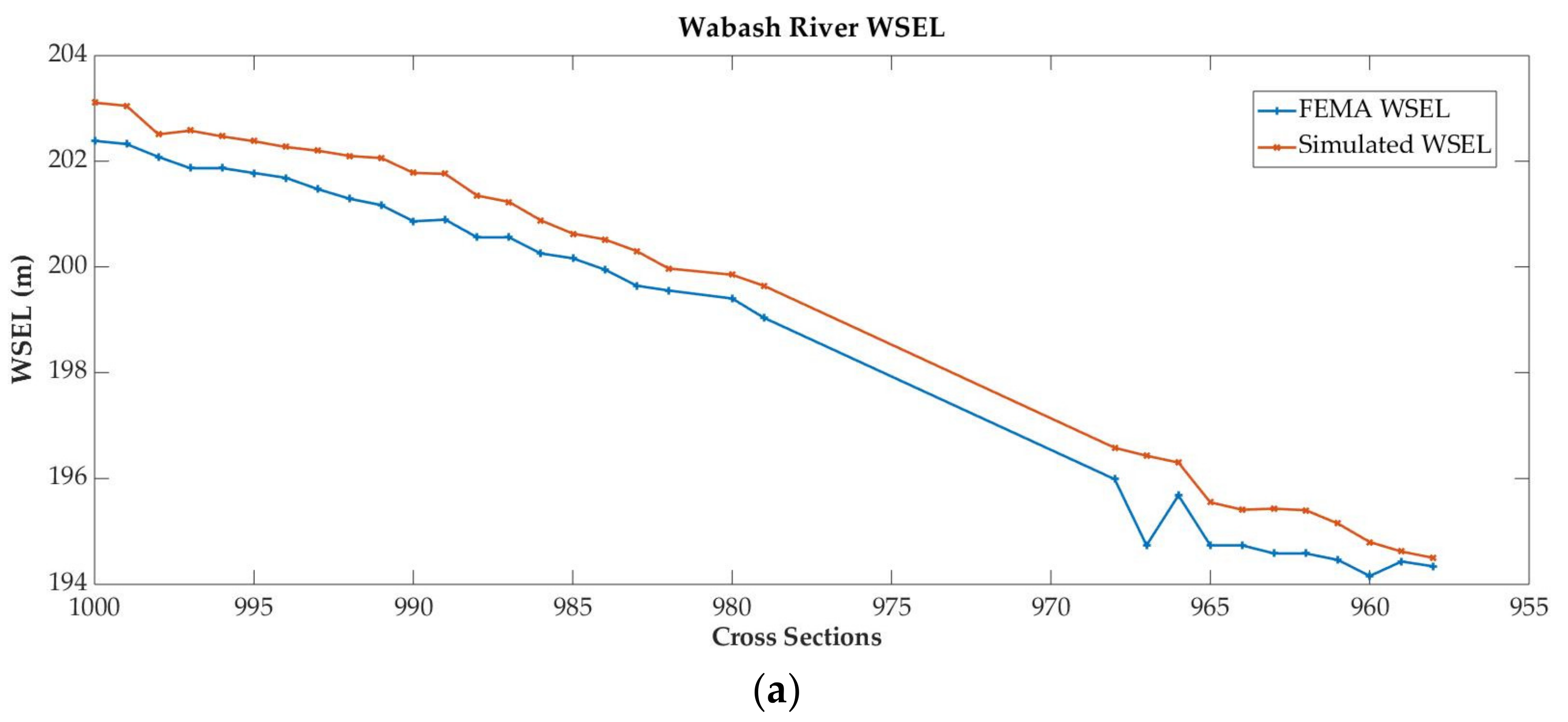
The Federal Emergency Management Agency (FEMA), established in 1968 in the US, is managing the national flood insurance program for an immediate response, which aims in decreasing the impacts of flooding disasters. FEMA has been conducting flood mapping on the areas prone to flooding. FEMA uses HEC-RAS to generate flood inundation maps using one-dimensional (1D) hydraulic modeling, which is helpful for programs that analyze flood risk and provide flood insurance [16]. For flood inundation mapping and additional inundation analysis, this study makes use of Civil GeoHECRAS. Many studies have utilized Civil GeoHECRAS for hazard, vulnerability, and risk assessment of flood zones with a conclusion that flood inundation mapping is a crucial step for flood risk management [17,18,19,20].
CMIP6 proposes a scenario model intercomparison project based on the Shared Socioeconomic Pathways (SSPs), and Representative Concentration Pathways (RCPs). It provides a database for relevant water resources questions and integrating multiple SSP scenarios into hydrological models allows a better understanding of climate and social influences on the physical processes of hydrological systems [
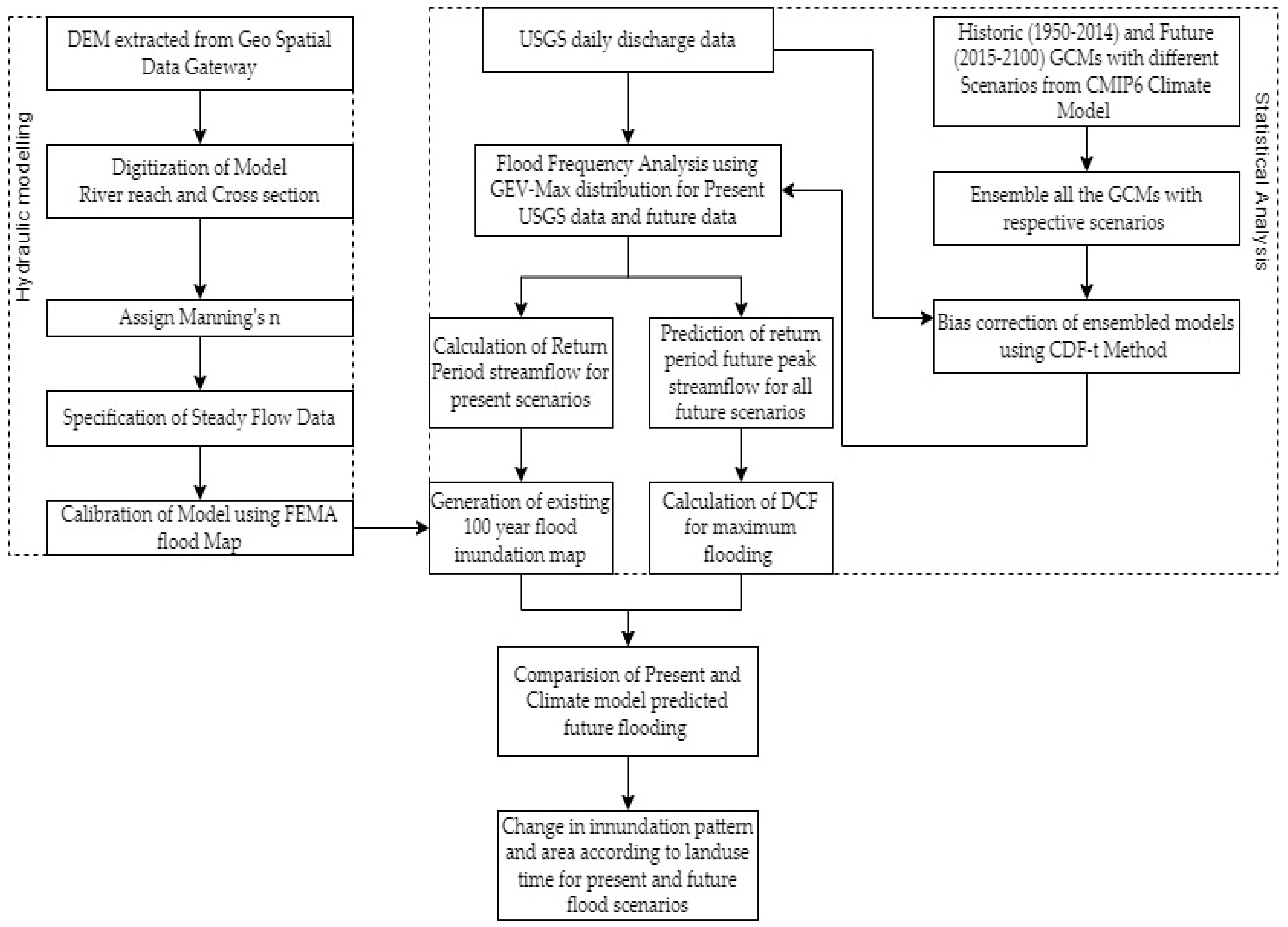
9]. The main goal of this study is to forecast potential future flood scenarios and analyze flood inundation extents utilizing the CMIP6 streamflow projection dataset for two different rivers, i.e., Wabash River and Fountain Creek. By examining the floodplain mapping and computing the severity of the inundation in both cases, the current flooding scenarios for various return times are contrasted with the future projected scenarios. By utilizing hydraulic modeling, a 100-year streamflow projection from CMIP6 was adopted as a design discharge. The novelty of the study is to forecast the extent of the floodplain in current and future climates using streamflow projection data from CMIP6. This study also provides an extensive analysis of the importance of flood forecast data. The major outcomes of this research work will be beneficial for offering responses to the inquiries as follows:
  • What effect will climate change have on streamflow in the future, and how would that modify the frequency of flooding?
  • What changes in flood size and pattern can be expected in the future under the estimated design discharge?
  • What are the changes in the future flood extent utilizing the CMIP6 climate model and how does it compare with the FEMA floodplain?
  • What changes in estimated inundation extent correspond to different land uses?
This study anticipates the significance of planning appropriate responses by utilizing projected future datasets to compare the extent of historical flooding. The region affected by extreme events is massively understated by current climate indicators. This study assesses the possibilities for future flooding to determine the extent of agricultural and urban flooding with an increase in river discharge. The findings of this study will allow policymakers to implement better water resource management policies and reduce risk by contemplating the likelihood of potential future flooding escalation.

2. Study Area and Dataset

2.1. Study Area

In the current study, Wabash River in Indiana and Fountain Creek in Colorado are considered to assess the changes in flooding patterns. A brief description of each reach is described below:

2.1.1. Wabash River

In this study, river reach from Wabash to Peru in Indiana was taken into consideration. Wabash River flows westward passing the cities, Huntington, Wabash, Logansport, and Lafayette, then southward to Terre Haute across Indiana. The total length of the study reach is 23.87 km. The study’s upstream portion begins at USGS Gage Station 03325000 in Wabash, which is located at latitude 40.79° N and longitude 85.82° W. The downstream portion of the study reach ends at USGS Gage station 033275000 in Peru, which is located at latitude of 40.75° N and longitude of 86.07° W (Figure 1). The Wabash River drains a total area of 85,860 square kilometers. The Wabash River is slow and muddy. The study region is dominated primarily by agricultural land and residential areas. The summer is warm, wet, and humid, and the winters are bitterly cold and windy. The highest temperature with an average high of 28.3 °C was recorded in June and the lowest temperature with an average low of −10 °C was recorded in January. The maximum rainfall with an annual average of 979.42 mm is observed in June.

2.1.2. Fountain Creek

Fountain Creek flows from Woodland Park in Teller County to the Arkansas River near Pueblo in Pueblo County, Colorado. In this study, the river reach from Pinon to Pueblo was taken into consideration. Fountain Creek is one of the tributaries of the Arkansas River, which is 119.9 km long with a great elevation difference of 1414.27 m to 4302.25 m, whereas the total length of the study reach is 17.03 km. The upstream of the study area is located near USGS Gage Station 07106300 situated at a latitude and longitude of 38.43° N and 104.59° W, respectively (Figure 2). The downstream portion of the study reach is close to USGS Gage Station 07106500, which has coordinates latitude and longitude of 38.28° N and 104.61° W, respectively. Summers are hot and clear, and winters are dry, cold, and cloudy. The highest temperature with an average high of 33.88 °C was recorded in July and the lowest temperature with an average low of −3.33 °C was recorded in December. August is the month that experiences the most precipitation, with an annual average of 330.71 mm of rain and 482.6 mm of snow.

2.2. Dataset

Several research institutes have been assisting in the development of climate datasets because of the connection between climate change and changes in hydrological and meteorological parameters. For the prediction of future flow for the study sites, this study uses river discharge data from the CMIP6 climate models dataset (downloaded from https://esgf-node.llnl.gov/search/cmip6/, retrieved on 10 March 2021). The study used CMIP6 scenarios with a greater number of GCMs for the reduction in uncertainties in the results [21]. The peak discharge for the study reach was determined using daily discharge data. The historical daily discharge data were taken from 1950 to 2014 from the USGS gage station upstream and downstream of the study reach. This current study utilized CMIP6 historical observations with a modeling period from 1950 to 2014. The gridded discharge data from CMIP6 were extracted at USGS gage stations. SSP1-2.6, SSP2-4.5, SSP3-7.0, and SSP5-8.5 were the four scenarios that were taken into consideration for future observation. The scenarios with two or more GCMs from 2015 to 2100 were adopted to evaluate future hydroclimatic change. In the current study, three models were opted for from a total of twelve models, with the remaining nine models being eliminated due to the availability of only one GCM. The preferred future scenarios consider anthropogenic factors in addition to socioeconomic changes. The scenarios and ensemble members used in the current study for each scenario are presented in Table 1.
In this study, for hydraulic modeling, 10 m resolution DEM was extracted from Geospatial Data Gateway (https://datagateway.nrcs.usda.gov/ accessed on 12 February 2021). The National Land Cover Dataset (NLCD) was utilized to acquire the land-use and land-cover data for Manning’s n value. To calibrate the model, the cross sections of the study reach were carefully selected along and between the cross sections of the FEMA flood extent. No structures such as levees and dams were considered due to the limitation of the detailed data of those structures. The range and assigned values for Manning’s n values are provided in Table 2. Different values for Manning’s n were considered for all the bank lines and centerlines. For the centerlines, Manning’s n considered throughout the channels in both study areas is 0.03. FEMA provides the flood map based on a 0.1% chance of flood, i.e., a 100-year flood map, which was utilized in this study for the calibration of the model. Calibration of the hydraulic models was performed with several assignments of Manning’s n value within the range provided by NLCD (Table 2). Manning’s n value of the final calibrated model was utilized for the future flood forecast.

3. Methodology

The current study involves (1) hydraulic analysis to generate flood inundation maps and (2) statistical analysis for the prediction of future design floods, which can be further utilized in other studies. Figure 3 shows the schematic diagram to generate existing and future 100-year flood maps.

3.1. Statistical Analysis

3.1.1. Bias Correction

The impact of climate change on hydrological and meteorological parameters has resulted in many research institutes to contribute in the generation of different climate datasets. CMIP6 climate model dataset acquires hydrological induced dataset which can be beneficial for the current study. Global time series datasets are available in Global Climate Model (GCM) datasets. The netCDF file of global time series data for river discharge was retrieved from the CMIP6 data. Using the global dataset, the time series of the river discharge at Wabash River and Fountain Creek were extracted. The purpose of the current study is to comprehend and assess the rise in river flooding caused by climate change; therefore, instead of using other concerning parameters such as precipitation, temperature, and wind speed, the study employs the river discharge data present in the CMIP6 datasets.
The data from the CMIP6 climate model has systematic biases. The bias correction of the CMIP6 models is important to further utilize the data for robust forecasting [22,23,24]. The GCMs for all scenarios were ensembled, and bias correction was performed using the CFD-t statistical technique [25,26,27,28]. The correlation between observed and modeled data was established in bias correction by employing the transformation function “T” as shown in Equation (1) below [26]. The future bias-corrected data (Fsh) were obtained from modeled future (Fgf) and historical climate data (Fgh). A range of bias corrections of Fgh and Fsh was determined. After obtaining the bias-corrected data, the computed CDF was utilized to predict future flows. The bias correction equations used are as follows:
T(FGh(x)) = Fsh(x)
Let us consider, u = FGh(x), which provides us x = F G h 1 (u) where uƐ [0, 1].
Then, Equation (1) can be modified as
T ( u ) = F s h ( F G h 1 ( u ) )
where T denotes the functional relationship that exists between the modeled and observed CDF results for the historical period.
The final CDF-t equation after validating Equation (2) is:
F s f ( x ) = F s h (   F G h 1 ( F G f ( x ) ) )

3.1.2. Flood Frequency Analysis and Future Design Flow

The Generalized Extreme Value (GEV) distribution was determined as being the best-fit among Gumbel distribution, Log Pearson III, and GEV-Max (L-Moments) distribution of the data using “Easyfit” software. Pearson Chi-square and Kolmogorov–Smirnov tests were performed as the fit criteria for fitting the best distribution. GEV obtains a higher ranking in between other approaches while the software itself performs the tests. For flood frequency analysis, (GEV) a parametric distribution was used that calculates the cumulative probability [29]. It is extensively utilized because of its capability to forecast streamflow and future extremes [24,29,30,31,32]. In earlier research, L-moment is used for the calculation of the parameters in the GEV distribution [24,29]. The GEV distribution for annual maxima is calculated using the following equation:
GEV   ( x : μ , σ , k ) = exp   { [ 1 + k ( x μ σ ) ] 1 k } if     k   o exp   { exp [ ( x μ σ ) ] 1 k } if     k = o
The location, scale, and shape of data are represented in Equation (4) by μ, σ, and k, respectively. For shape parameter k > 0, μσ/k < x < ∞; k = 0, −∞_ < x < ∞; k < 0, ∞_ < x < μσ/k [29]. L-moments, shape, scale, and locations are used for the GEV distribution parameters.
GEV was implemented in the current study to determine design streamflow at multiple recurrence intervals. The annual peak was determined for the historical data from 1950 to 2014. Annual peak discharge of each multimodel ensemble scenario (SSP1-2.6, SSP2-4.5, SSP3-7.0, SSP4-6.0, and SSP5-8.5) of the bias-corrected data was calculated from 2015 to 2100. The peak flows for various year return periods was used to determine the peak flow in the future. Peak flow was calculated for the CMIP6 climate model as well as observed data for 100-year and 500-year. For the future streamflow forecast, the Delta Change Factor (DCF) was used. The DCF method is a statistical downscaling method that is based on the idea to match the historical gage streamflow data and future streamflow data [33]. A main advantage of the DCF method is that historical patterns of temporal and spatial variability from the gridded observations are maintained, and comparison between future scenarios and historical data is straightforward and can be easily analyzed as shown in Equations (5) and (6). The streamflow estimated by FEMA using the DCF represents a flood under stationary conditions. In the current study, for each scenario and return period, DCF is calculated. In order to leverage the largest possible rise in flood data in the future, a greater value of DCF is taken into consideration for this study.
DCF = Daily   maximum   from   future   model Daily   maximum   from   the   Historic   model =   Δ Q = Q f , m a x Q h , m a x  
where ΔQ is the delta change factor for the peak discharge; Qf,max is the daily maximum from future model and Qh is the modeled historical peak discharge.
  Peak   Future   Flow = DCF   × Existing   Peak   Flow

3.2. Hydraulic Modelling

The flood map obtained from the current study was compared with the 100-year and 500-year FEMA flood scenarios to study how the future climate may affect flooding. In the Civil GeoHECRAS 1D hydraulic modeling simulation, the 100-year streamflow projection from CMIP6 was adopted as a design discharge. Civil GeoHECRAS is used as Hydraulic modelling tool for floodplain inundation mapping. DEM was used for the terrain data in the Civil GeoHECRAS 1D simulation model. The reach of the river with upstream and downstream USGS gage stations was selected for the study. River reach, banks, and cross sections at intervals and bends were drawn utilizing the tools available in GeoHECRAS. Each cross-section, the river channel, and banks were provided the default Manning’s n values based upon the land use on the cross sections. Land use for the Manning’s n was extracted from National Land Cover Data (NLCD). The Manning’s coefficients considered for the simulation vary for bank lines, but 0.03 was taken for the river’s centerline. The calibration of the hydraulic model made utilization of water surface elevations (WSELs) from FEMA. The modeled cross sections were compared with observed WSEL obtained from FEMA. The flood inundation maps are prepared for bias-corrected historical data and future projected data after the calibration of the model. The model’s efficiency was evaluated using a range of statistical indicators, including Nash–Sutcliffe Efficiency (NSE), Root Mean Square Error (RMSE), Coefficient of Determination (R2), and Percent Bias (PBIAS) [34].
Peak streamflow derived from GEV for 100-year and 500-year periods were utilized in Civil GeoHECRAS for 1D steady flow hydraulic modeling. The river network of both study reaches were modeled in Civil GeoHECRAS using geometric data and hydraulic computation. In this study, the ratio of peak flow downstream and upstream was assumed to remain constant. Among all the DCFs, the highest DCF was selected for the highest increase in future flood conditions. Spatial flood extents and depth were obtained using the future peak streamflow.

4. Results

4.1. Hydraulic Modelling and Flood Frequency Analysis

In the current study, data from the USGS gage station, DEM, land use land cover, and CMIP6 streamflow data were utilized to develop future flood maps. The annual peak flows obtained from the USGS station are shown in Figure 4. The annual peak flows from 3-GCMs with 75 different streamflow projections from CMIP6 models was used showing an increasing trend of streamflow in both the Wabash River and Fountain Creek. Historical data were utilized for bias correction of multimodel ensembled GCMs for all CMIP6 future scenarios. The scenarios SSP1-2.6, SSP 2-4.5, SSP3-7.8, and SSP5-8.5 were used in the current study.
For both study reach, the best-fit distribution was established using the Easyfit tool, which was used to compute design peak flows at varied recurrence intervals for all future scenarios. Peak flows at different return periods (2-year, 5-year, 10-year, 50-year, 100-year, and 500-year) with their respective scenarios and observed flow are presented in Table 3 and Table 4 for the Wabash River and Fountain Creek, respectively. In this study, a 100-year return period was considered as design discharge for flood mapping.
The peak discharge for the Wabash River was determined to be 1313 m3/s for SSP1-2.6, 1465 m3/s for SSP2-4.5, 1522 m3/s for SSP3-7.0, and 1511 m3/s for SSP5-8.5. The peak discharge for Fountain Creek was determined to be 12,865 m3/s for SSP1-2.6, 13,614 m3/s for SSP2-4.5, 12,444 m3/s for SSP3-7.0, and 14,731 m3/s for SSP5-8.5. In Figure 5a, we can observe that SSP3-7.0 has higher values for the Wabash River, and in Figure 5b SSP 5-8.5 for Fountain Creek. The DCF was computed for each scenario using the CMIP6 climate model’s varying return period discharge and the FEMA 100-year flood discharge.
Table 5 compares the DCF values of several SSP scenarios for 100-year and 500-year flood occurrences. For each scenario, DCF was computed for future CMIP6 model discharge and FEMA 100-year flood discharge. The DCF values greater than 1 infer a higher risk of flood in the future. The 100-year DCF value is lower for SSP1-2.6 (1.10) and highest for scenario SSP3-7.0 in the Wabash River whereas SSP3-7.0 (11.20) was observed to be lower in Fountain Creek (Table 5). All the scenarios were found to have DCF values greater than 1, suggesting that runoff will increase in the future in both Wabash River and Fountain Creek. It can be observed in Table 5, that Fountain Creek has the highest DCF value in SSP 5-8.5 scenario. Similarly, for the Wabash River, SSP3-7.0 has the highest DCF in 100-year (1.28) than that of SSP 1-2.6, SSP 2-4.5, and SSP5-8.5, suggesting an increase in the future runoffs which may be resulting from future land-use changes, and higher GHG emissions.

4.2. Statistical Performance of Hydraulic Modeling

One-dimensional hydraulic modeling in GeoHECRAS was performed after establishing the DCF values and peak discharge for a 100-year and 500-year return period. The WSEL generated from USGS peak flow data in GeoHECRAS was compared with the FEMA WSEL for calibrating the 100-year design flood. Calibration of observed and simulated WSEL was performed to establish a robust hydraulic model using statistical indicators such as NSE, RMSE, R2, and PBIAS [35]. The simulated and actual WSEL of Wabash River and Fountain Creek for the chosen cross sections are shown in Figure 6a,b, respectively. Calibration of observed and simulated WSEL was performed to establish a robust hydraulic model using statistical indicators such as NSE, RMSE, R2, and PBIAS. The values for NSE, RMSE, R2, and PBIAS of the calibrated model were found to be 0.94, 0.12, 0.99, and −0.33, respectively, for Wabash River, and 0.99, 0.17, 0.99, and 0.06 for Fountain Creek. The resulting NSE value is close to one, suggesting that the observed and simulated WSEL nearly match. Furthermore, the RMSE values indicate that the observed and simulated WSEL has a very small error. The R2 value found indicates that the observed and simulated WSEL are closely matched with minor dispersion. The negative value of PBIAS indicates that biases are overestimated. The statistical indicators for the robustness of the calibrated hydraulic model were judged to be within an acceptable range. The calibrated model was validated, and a CMIP6 model with a high peak discharge was used to forecast future 100-year and 500-year WSEL, and flood inundation maps were developed.

4.3. Flood Inundation Mapping

Flood extent maps for the study area of Wabash River and Fountain Creek were prepared using historical USGS gage data which is demonstrated in Figure 7 and Figure 8 below. The maps were calibrated using the FEMA flood map for 100-year return period. It is evident in the flood extent map of Wabash River and Fountain Creek shows the inundation areas are calibrated close to the FEMA flood maps.
The calibrated and validated GeoHECRAS model was employed for the generation of flood inundation maps. The peak discharge with the highest DCF was utilized for the 100-year future flood inundation mapping. FEMA flood maps were compared with the spatial extent of the flood inundation map derived from the climate model. It was observed in Figure 9a,b that the spatial extent of the future 100-year map has a higher footprint than that of the current 100-year FEMA flood map. The future peak discharge and DCF values were found to be higher than the observed USGS discharge and it can be observed that more land would be inundated by a future 100-year flood than by the FEMA flood footprint. This demonstrates the critical urgency for the appropriate study of both study areas for flood management strategies and future flood studies. Figure 10a,b show the comparison of 100-year return period flood inundation maps provided by USGS data and CMIP6 climate model data for the Wabash River and Fountain Creek.

4.4. Change in Flood Inundation in Different Land Use

From the current study, it is evident that discharge will increase in the future, which will have flooding impacts on different land use. Numerous variables including hydrological parameters, morphological characteristics, land use, and the chosen numerical model, affect the calculation of flooding areas in a basin. Each basin is different, thus it must be carefully analyzed while taking into consideration all of the aforementioned aspects [36]. Land use changes with time, and with increased urban development, more impervious surfaces will increase replacing open space and barren lands. This leads to more surface runoff and flash floods. An increase in inundation extent can be observed in 100-year future predicted floods. In both the study reaches, if the land use remains the same, the increase in the inundation area is very high. Comparatively, the current 100-year flood is less disastrous than the expected future 100-year design flood.
The changes in the area according to the land use for both study areas, Wabash River and Fountain Creek, are demonstrated in Table 6 and Table 7, respectively. In both cases, developed land is more at risk than open space or cultivated land. This can have a direct impact on property, human life, and the environment. The increased percentage is significantly higher for the developed area, which demonstrates the requirement of strategic planning by considering climate change and anthropogenic activities.

5. Discussion

A river’s surge over its typical flow depth is seen to have an impact on human habitation areas. Rivers are becoming narrower and settlement areas are growing as a consequence of increased human activity. Increased civilization has led to urbanization and industrialization, which have altered the environment and contributed to flooding in various parts of the world. Flooding has been a recurring natural disaster in many areas which has been causing loss of human life, and destruction of habitat, environment, and economical status. With the increasing population density near water bodies and changing climate, flood vulnerability can be expected soon in the upcoming years. Future floodplain management is essential to protect life and property for which future flood mapping can be an effective tool. In this study, two different rivers, i.e., one slow-moving large Wabash River and one fast-moving small fountain creek were considered. As observed from the findings of the current study, populations residing near the water bodies are vulnerable to changes in streamflow causing severe damage to their day-to-day activities.
For the determination of a suitable probability distribution method, the Easyfit tool was utilized. Kolmogorov–Smirnov and Pearson Chi-Square tests were used to determine the distribution that well-suited the data. The best-fit distribution data were determined by GEV Max (L-Moment). The proper distribution of the data for the flood frequency analysis must be determined to avoid possible errors [37].
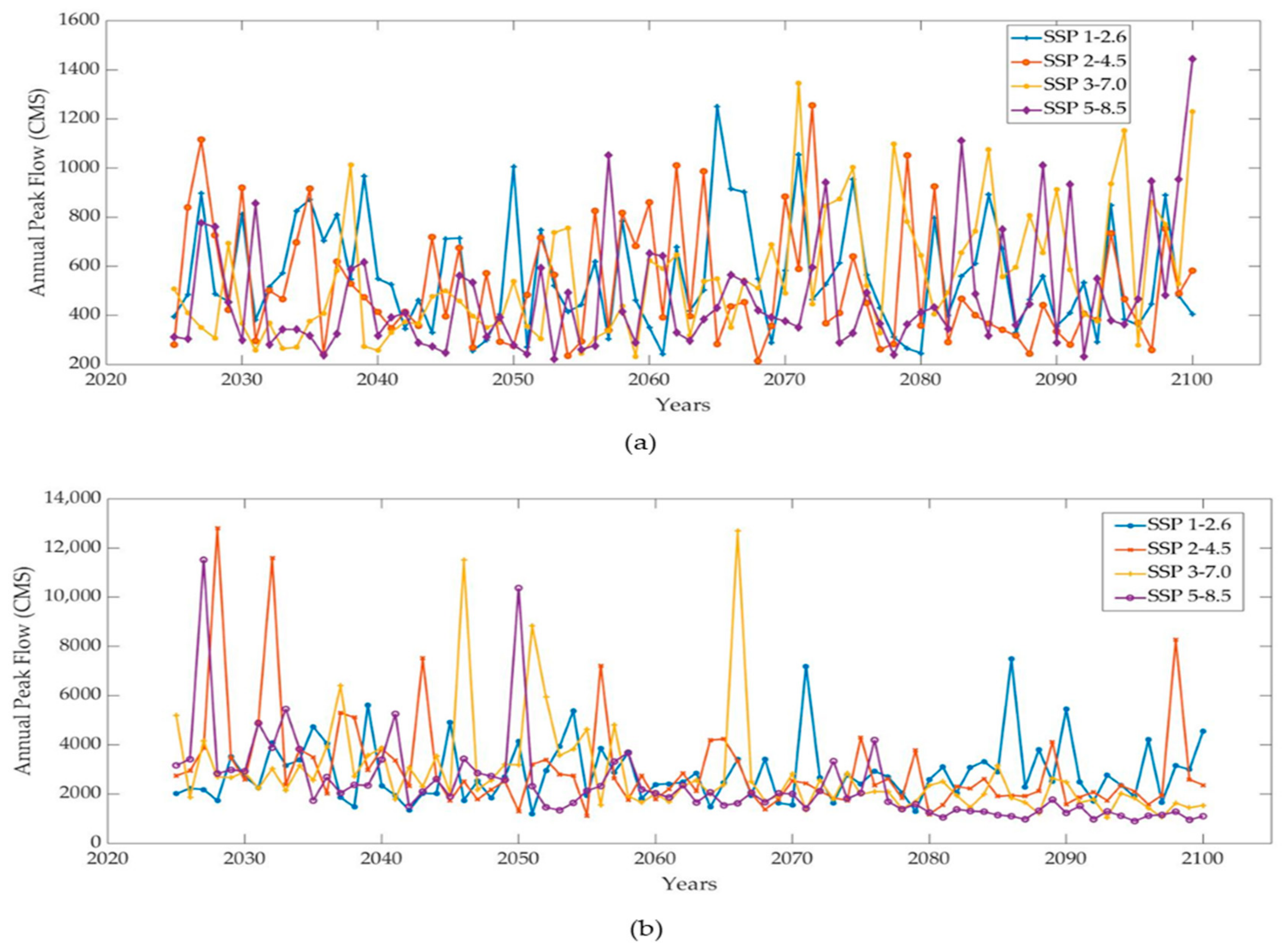
This study utilizes the CMIP6 model for the streamflow future projection. Future streamflow was evaluated using the different emission scenarios of CMIP6 streamflow projection with their different SSPs and forcing levels. This will help us in the study of climatic and societal change with an extensive array of streamflow [
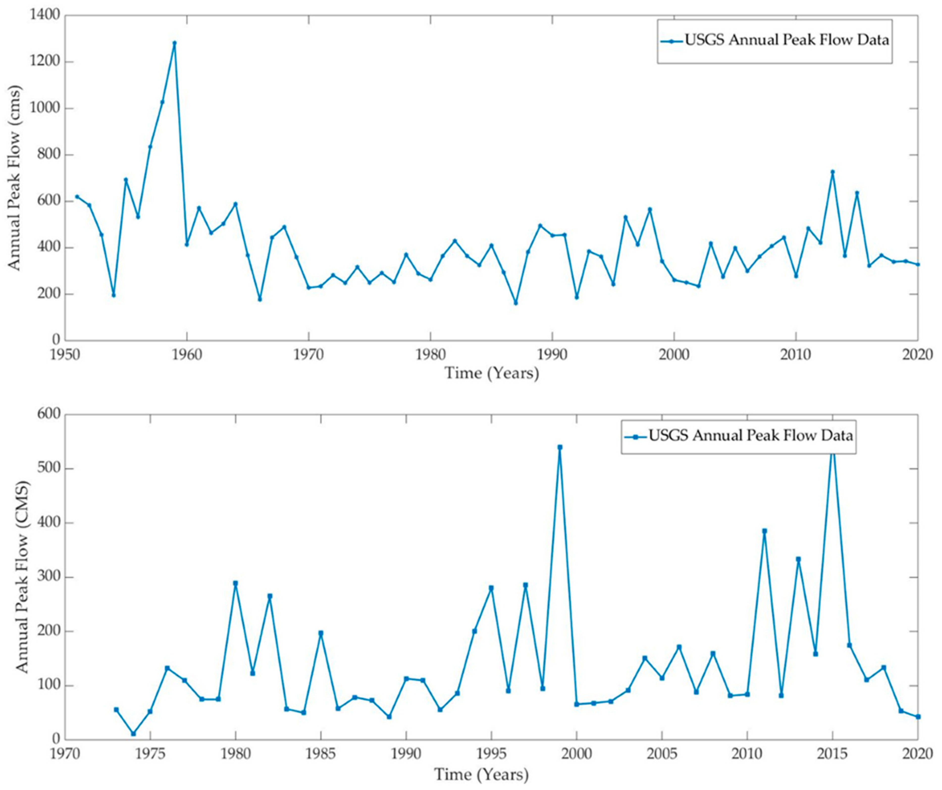
38]. After bias correction and downscaling, the CMIP6 climate model dataset reveals an increase in the flood flow regime in the future (2015–2100) compared with the historical period (1950–2014). Increases in the values were seen for both the annual peak discharge and the monthly peak discharge. This outcome is consistent with earlier studies, which also included an examination of flood change based on precipitation and temperature datasets. There is evidence for an ascending tendency for the yearly peak flow in the near term and a little descending trend for the long term [39]. In the current study, we can observe an increase in peak flow in the future aligning with the studies and always showcasing the increasing trend on future peak flow.
In the current study, it can be observed that all the DCF values that are greater than 1 suggest that there is an increment in the future design flow in all scenarios. The highest DCF was used to predict the maximum flooding extent in both the study reaches [40,41]. In past literature on climate science, max DCF was used. An increased DCF in the future results in an increased design flood for both the study reaches. The maximum DCF value with the highest probability of a rise in the future design flood is shown in Scenario SSP 5-8.5; therefore, the highest DCF was considered for the estimation of the future design flood. DCF was calculated and floodplain maps were prepared for the selected future scenarios using the Civil GeoHECRAS 1D model. Higher values for future floods were observed in both the study reaches than that of FEMA. A very large increase in streamflow is observed for Fountain Creek in comparison to the Wabash River. This demonstrates that the regular flash floods that happen in the Fountain Creek watershed can result in significant flooding events with significantly increased hazards. There is a significant human population in the study reach the region, which puts it at risk of flooding [15,42,43].
Researchers have previously found that climate change impacts and changes in land use may alter the risk of the extent of the floodplain [21,24]. Comparatively, the increase in streamflow for the Wabash River is less than that of Fountain Creek. However, this does not imply that the streamflow will not rise in the future. The agricultural region is more vulnerable to flooding in the future than it is today along the Wabash River. Local authorities can utilize the current study’s findings of projected future flood inundation maps to help them plan for probable future flood dangers. The massive change in flood inundation areas from present and future forecasted floods can be observed. To reduce the flood hazards due to the changing climate, planners and engineers should take projected streamflow into account. This demands the requirement of proper management of floods to minimize future hazardous situations. Policymakers, engineers, climatologists, and managers of water resources can consider the area underwater in the future when planning and building infrastructure that will help mitigate the unanticipated risk of floods and floodplains caused by climate change.

6. Conclusions

Changing climate in the current and future conditions have a great risk of hydrological extremes which are increasing and are predicted to increase continuously in the coming future. Different agencies are applying multiple approaches designed for the mitigation of hydrological extremes but climate change as the key factor is being missed while developing strategies. To maximize the performance of hydraulic structures built for a certain life span of the design period, future streamflow forecasts were used. This will help in the minimization of the casualties that may occur in life, and environmental and financial sectors due to the failure of hydraulic structures. The results may not be similar for all the watersheds, but this kind of study can be beneficial for the study in other watersheds as well.
The following significant points serve as a summary of this study:
  • The best-fit distribution was found as GEV-Max (L-Moments) using the simple fit program, which conducts both Pearson Chi-square and Kolmogorov–Smirnov tests;
  • The peak flow was calculated using GEV-Max (L-Moments) for a 100-year return period;
  • Different multimodal climate scenarios were ensembled and compared with historical data for bias correction;
  • All the calculated DCFs were more than 1 suggesting an increase in future design flow with non-stationary behavior in both the study areas;
  • Future scenario SSP 5-8.5 is predicted as a maximum increase in peak flow for a 100-year return period;
  • GeoHECRAS 1D steady modeling was utilized for floodplain mapping simulation, demonstrating that the projected 100-year scenario exceeds the FEMA 100-year peak flow;
  • The urban settlements along the creek are at higher risk than other land use.
A design flood is considered for the design of hydraulic structures. This study highlights the significance of climate data and flood design patterns in the future. This study demonstrates how past and future CMIP6 climate data may be used to look forward to streamflow in the future. Thus, observed streamflow was used for developing floodplain inundation maps. The design of the structures considering the forecasted streamflow will help reduce the risk of future flooding. The results from this study can be useful to policymakers in the future when a climate change factor is needed for flood extent analysis. The framework applied in this study of Wabash River and Fountain Creek for the future flood forecasting can be used for other research as per the requirements.

Author Contributions

Conceptualization, A.K.; formal analysis, S.P.; investigation, S.P.; software, S.P.; supervision, A.K.; writing—original draft, S.P.; and A.K.; writing—review and editing, S.P.; N.J.; and A.K. All authors have read and agreed to the published version of the manuscript.

Funding

This research received no external funding.

Institutional Review Board Statement

Not applicable.

Informed Consent Statement

Not applicable.

Data Availability Statement

The World Climate Research Programme Coupled Model Intercomparison Project provides the CMIP6 model data utilized in this study. (https://esgf-node.llnl.gov/projects/cmip6/, accessed on 10 March 2021).

Conflicts of Interest

The authors declare no conflict of interest.

References

  1. Merz, B.; Aerts, J.; Arnbjerg-Nielsen, K.; Baldi, M.; Becker, A.; Bichet, A.; Blöschl, G.; Bouwer, L.M.; Brauer, A.; Cioffi, F.; et al. Floods and Climate: Emerging Perspectives for Flood Risk Assessment and Management. Nat. Hazards Earth Syst. Sci. 2014, 14, 1921–1942. [Google Scholar] [CrossRef]
  2. Easterling, D.R.; Meehl, G.A.; Parmesan, C.; Changnon, S.A.; Karl, T.R.; Mearns, L.O. Climate Extremes: Observations, Modeling, and Impacts. Sci. New Ser. 2000, 289, 2068–2074. [Google Scholar] [CrossRef] [PubMed]
  3. Ogunbode, C.A.; Doran, R.; Böhm, G. Exposure to the IPCC Special Report on 1.5 °C Global Warming Is Linked to Perceived Threat and Increased Concern about Climate Change. Clim. Chang. 2020, 158, 361–375. [Google Scholar] [CrossRef]
  4. O’Neill, B.C.; Tebaldi, C.; van Vuuren, D.P.; Eyring, V.; Friedlingstein, P.; Hurtt, G.; Knutti, R.; Kriegler, E.; Lamarque, J.-F.; Lowe, J.; et al. The Scenario Model Intercomparison Project (ScenarioMIP) for CMIP6. Geosci. Model Dev. 2016, 9, 3461–3482. [Google Scholar] [CrossRef]
  5. Middelkoop, H.; Daamen, K.; Gellens, D.; Grabs, W.; Kwadijk, J.C.J.; Lang, H.; Schulla, J.; Wilke, K. Impact of Climate Change on Hydrological Regimes and Water Resources Management in the Rhine Basin. Clim. Chang. 2001, 49, 105–128. [Google Scholar] [CrossRef]
  6. Roy, L.; Leconte, R.; Brissette, F.P.; Marche, C. The Impact of Climate Change on Seasonal Floods of a Southern Quebec River Basin. Hydrol. Process. 2001, 15, 3167–3179. [Google Scholar] [CrossRef]
  7. Arnell, N.W.; Gosling, S.N. The Impacts of Climate Change on River Flood Risk at the Global Scale. Clim. Chang. 2016, 134, 387–401. [Google Scholar] [CrossRef]
  8. Hirabayashi, Y.; Kanae, S.; Emori, S.; Oki, T.; Kimoto, M. Global Projections of Changing Risks of Floods and Droughts in a Changing Climate. Hydrol. Sci. J. 2008, 53, 754–772. [Google Scholar] [CrossRef]
  9. Quan, X.-W.; Hoerling, M.; Smith, L.; Perlwitz, J.; Zhang, T.; Hoell, A.; Wolter, K.; Eischeid, J. Extreme California Rains During Winter 2015/16: A Change in El Niño Teleconnection? Bull. Am. Meteorol. Soc. 2018, 99, S49–S53. [Google Scholar] [CrossRef]
  10. De Paola, F.; Giugni, M.; Pugliese, F.; Annis, A.; Nardi, F. GEV Parameter Estimation and Stationary vs. Non-Stationary Analysis of Extreme Rainfall in African Test Cities. Hydrology 2018, 5, 28. [Google Scholar] [CrossRef]
  11. Alfieri, L.; Feyen, L.; Dottori, F.; Bianchi, A. Ensemble Flood Risk Assessment in Europe under High End Climate Scenarios. Glob. Environ. Chang. 2015, 35, 199–212. [Google Scholar] [CrossRef]
  12. Sankarasubramanian, A.; Vogel, R.M. Hydroclimatology of the Continental United States: U.S. HYDROCLIMATOLOGY. Geophys. Res. Lett. 2003, 30, 1363. [Google Scholar] [CrossRef]
  13. Rao, A.; Al-Wagdany, A. Effects of Climatic Change in Wabash River Basin. J. Irrig. Drain. Eng. 1995, 121, 207–215. [Google Scholar] [CrossRef]
  14. Zhang, Y.-K.; Schilling, K.E. Increasing Streamflow and Baseflow in Mississippi River since the 1940s: Effect of Land Use Change. J. Hydrol. 2006, 324, 412–422. [Google Scholar] [CrossRef]
  15. Gochis, D.; Schumacher, R.; Friedrich, K.; Doesken, N.; Kelsch, M.; Sun, J.; Ikeda, K.; Lindsey, D.; Wood, A.; Dolan, B.; et al. The Great Colorado Flood of September 2013. Bull. Am. Meteorol. Soc. 2015, 96, 1461–1487. [Google Scholar] [CrossRef]
  16. Ashley, S.T.; Ashley, W.S. Flood Fatalities in the United States. J. Appl. Meteorol. Climatol. 2008, 47, 805–818. [Google Scholar] [CrossRef]
  17. Bathi, J.; Das, H. Vulnerability of Coastal Communities from Storm Surge and Flood Disasters. Int. J. Environ. Res. Public Health 2016, 13, 239. [Google Scholar] [CrossRef]
  18. Tingsanchali, T.; Karim, F. Flood-Hazard Assessment and Risk-Based Zoning of a Tropical Flood Plain: Case Study of the Yom River, Thailand. Hydrol. Sci. J. 2010, 55, 145–161. [Google Scholar] [CrossRef]
  19. Mihu-Pintilie, A.; Cîmpianu, C.I.; Stoleriu, C.C.; Pérez, M.N.; Paveluc, L.E. Using High-Density LiDAR Data and 2D Streamflow Hydraulic Modeling to Improve Urban Flood Hazard Maps: A HEC-RAS Multi-Scenario Approach. Water 2019, 11, 1832. [Google Scholar] [CrossRef]
  20. Klijn, F.; Kreibich, H.; de Moel, H.; Penning-Rowsell, E. Adaptive Flood Risk Management Planning Based on a Comprehensive Flood Risk Conceptualisation. Mitig. Adapt. Strateg. Glob. Chang. 2015, 20, 845–864. [Google Scholar] [CrossRef]
  21. Eyring, V.; Bony, S.; Meehl, G.A.; Senior, C.A.; Stevens, B.; Stouffer, R.J.; Taylor, K.E. Overview of the Coupled Model Intercomparison Project Phase 6 (CMIP6) Experimental Design and Organization. Geosci. Model Dev. 2016, 9, 1937–1958. [Google Scholar] [CrossRef]
  22. Nohara, D.; Kitoh, A.; Hosaka, M.; Oki, T. Impact of Climate Change on River Discharge Projected by Multimodel Ensemble. J. Hydrometeorol. 2006, 7, 1076–1089. [Google Scholar] [CrossRef]
  23. Shrestha, A.; Rahaman, M.M.; Kalra, A.; Jogineedi, R.; Maheshwari, P. Climatological Drought Forecasting Using Bias Corrected CMIP6 Climate Data: A Case Study for India. Forecasting 2020, 2, 59–84. [Google Scholar] [CrossRef]
  24. Sillmann, J.; Kharin, V.V.; Zwiers, F.W.; Zhang, X.; Bronaugh, D. Climate Extremes Indices in the CMIP5 Multimodel Ensemble: Part 2. Future Climate Projections. J. Geophys. Res. Atmos. 2013, 118, 2473–2493. [Google Scholar] [CrossRef]
  25. Guo, L.-Y.; Gao, Q.; Jiang, Z.-H.; Li, L. Bias Correction and Projection of Surface Air Temperature in LMDZ Multiple Simulation over Central and Eastern China. Adv. Clim. Chang. Res. 2018, 9, 81–92. [Google Scholar] [CrossRef]
  26. Michelangeli, P.-A.; Vrac, M.; Loukos, H. Probabilistic Downscaling Approaches: Application to Wind Cumulative Distribution Functions. Geophys. Res. Lett. 2009, 36, L11708. [Google Scholar] [CrossRef]
  27. Pierce, D.W.; Cayan, D.R.; Maurer, E.P.; Abatzoglou, J.T.; Hegewisch, K.C. Improved Bias Correction Techniques for Hydrological Simulations of Climate Change. J. Hydrometeorol. 2015, 16, 2421–2442. [Google Scholar] [CrossRef]
  28. Famien, A.M.; Janicot, S.; Ochou, A.D.; Vrac, M.; Defrance, D.; Sultan, B.; Noël, T. A Bias-Corrected CMIP5 Dataset for Africa Using the CDF-t Method—A Contribution to Agricultural Impact Studies. Earth Syst. Dynam. 2018, 9, 313–338. [Google Scholar] [CrossRef]
  29. Hosking, J.R.M. L-Moments: Analysis and Estimation of Distributions Using Linear Combinations of Order Statistics. J. R. Stat. Soc. Ser. B 1990, 52, 105–124. [Google Scholar] [CrossRef]
  30. Santos, E.B.; Lucio, P.S.; Santos e Silva, C.M. Estimating Return Periods for Daily Precipitation Extreme Events over the Brazilian Amazon. Theor. Appl. Climatol. 2016, 126, 585–595. [Google Scholar] [CrossRef]
  31. Hosking, J.R.M.; Wallis, J.R.; Wood, E.F. Estimation of the Generalized Extreme-Value Distribution by the Method of Probability-Weighted Moments. Technometrics 1985, 27, 251–261. [Google Scholar] [CrossRef]
  32. Hamzah, F.M.; Yusoff, S.H.; Jaafar, O. L-Moment-Based Frequency Analysis of High-Flow at the Sungai Langat, Kajang, Selangor, Malaysia. Sains Malays. 2019, 48, 1357–1366. [Google Scholar] [CrossRef]
  33. Navarro-Racines, C.; Tarapues, J.; Thornton, P.; Jarvis, A.; Ramirez-Villegas, J. High-Resolution and Bias-Corrected CMIP5 Projections for Climate Change Impact Assessments. Sci. Data 2020, 7, 7. [Google Scholar] [CrossRef]
  34. Joshi, N.; Bista, A.; Pokhrel, I.; Kalra, A.; Ahmad, S. Rainfall-Runoff Simulation in Cache River Basin, Illinois, Using HEC-HMS. In Proceedings of the World Environmental and Water Resources Congress, Pittsburgh, PA, USA, 19–23 May 2019; American Society of Civil Engineers: Pittsburgh, PA, USA, 2019; pp. 348–360. [Google Scholar]
  35. Majone, B.; Avesani, D.; Zulian, P.; Fiori, A.; Bellin, A. Analysis of High Streamflow Extremes in Climate Change Studies: How Do We Calibrate Hydrological Models? Hydrol. Earth Syst. Sci. 2022, 26, 3863–3883. [Google Scholar] [CrossRef]
  36. Apollonio, C.; Balacco, G.; Novelli, A.; Tarantino, E.; Piccinni, A. Land Use Change Impact on Flooding Areas: The Case Study of Cervaro Basin (Italy). Sustainability 2016, 8, 996. [Google Scholar] [CrossRef]
  37. Re, M.; Barros, V.R. Extreme Rainfalls in SE South America. Clim. Chang. 2009, 96, 119–136. [Google Scholar] [CrossRef]
  38. Li, H.; Sheffield, J.; Wood, E.F. Bias Correction of Monthly Precipitation and Temperature Fields from Intergovernmental Panel on Climate Change AR4 Models Using Equidistant Quantile Matching. J. Geophys. Res. 2010, 115, D10101. [Google Scholar] [CrossRef]
  39. Xiang, Y.; Wang, Y.; Chen, Y.; Zhang, Q. Impact of Climate Change on the Hydrological Regime of the Yarkant River Basin, China: An Assessment Using Three SSP Scenarios of CMIP6 GCMs. Remote Sens. 2021, 14, 115. [Google Scholar] [CrossRef]
  40. Nyaupane, N.; Thakur, B.; Kalra, A.; Ahmad, S. Evaluating Future Flood Scenarios Using CMIP5 Climate Projections. Water 2018, 10, 1866. [Google Scholar] [CrossRef]
  41. Pokhrel, I.; Kalra, A.; Rahaman, M.M.; Thakali, R. Forecasting of Future Flooding and Risk Assessment under CMIP6 Climate Projection in Neuse River, North Carolina. Forecasting 2020, 2, 323–345. [Google Scholar] [CrossRef]
  42. Yochum, S.E. Colorado Front Range Flood of 2013: Peak Flows and Flood Frequencies. In Proceedings of the 3rd Joint Federal Interagency Conference on Sedimentation and Hydrologic Modeling, Reno, NV, USA, 19 April 2015. [Google Scholar] [CrossRef]
  43. Hollis, G.E. The Effect of Urbanization on Floods of Different Recurrence Interval. Water Resour. Res. 1975, 11, 431–435. [Google Scholar] [CrossRef]
Figure 1. Map of study reach Wabash River in Indiana: (a) Map of United States; (b) location of Wabash and Miami County (purple) in Indiana; (c) Wabash River crossing Miami and Wabash County; and (d) study reach with upstream (located at Wabash) and downstream (located at Peru) USGS gage station.
Forecasting 05 00022 g001
Figure 2. Map of study reach, Fountain Creek in Colorado: (a) Map of United States; (b) location of Pueblo County (purple) in Colorado; (c) Fountain Creek crossing Pueblo County; and (d) study reach with upstream and downstream USGS gage station.
Forecasting 05 00022 g002
Figure 3. Schematic representation of the procedures used in the study.
Forecasting 05 00022 g003
Figure 4. Historical annual peak streamflow dataset of Wabash River (top) and Fountain Creek (bottom).
Forecasting 05 00022 g004
Figure 5. (a) SSP scenarios of annual peak future streamflow of Wabash River. (b) SSP scenarios of annual peak future streamflow of Fountain Creek.
Forecasting 05 00022 g005
Figure 6. Calibration plot between FEMA WSEL and simulated WSEL of (a) Wabash River and (b) Fountain Creek.
Forecasting 05 00022 g006aForecasting 05 00022 g006b
Figure 7. Flood extent comparison between FEMA 100-year and historical (USGS) data for Wabash River.
Forecasting 05 00022 g007
Figure 8. Flood extent comparison between FEMA 100-year and historical (USGS) data for Fountain Creek.
Forecasting 05 00022 g008
Figure 9. Comparison between FEMA 100-year and CMIP6 100-year flood extent footprint of (a) Wabash River; (b) Fountain Creek.
Forecasting 05 00022 g009
Figure 10. Comparison of 100-year return period flood inundation maps provided by USGS data and CMIP6 climate model data of (a) Wabash River and (b) Fountain Creek.
Forecasting 05 00022 g010
Table 1. Modeling institution and number of ensemble members of each climate model.
ScenariosModeling Institution
ModelsHistoricalSSP1-2.6SSP2-4.5SSP3-7.0SSP5-8.5
CNRM-CM6246665CNRM-CFRFACS
CNRM-ESM255555CNRM-CFRFACS
CNRM-CM6-HR11111CNRM-CFRFACS
Table 2. Manning’s n values of flow areas utilized for Wabash River and Fountain Creek.
NLCD CodeLand CoverAllowable Manning’s RangeAssigned Manning’s n
Wabash RiverFountain Creek
11Open Water0.025–0.0500.0300.030
21Developed, Open Space0.030–0.0500.0400.045
22Developed, Low Density0.050–0.1200.0800.075
23Developed, Medium Density0.060–0.1400.100.120
24Developed, High Density0.080–0.2000.1200.120
31Undeveloped, Barren Land0.025–0.0350.0300.035
71Undeveloped, Grassland0.025–0.0500.0350.045
52Undeveloped, Shrub/Scrub0.070–0.1600.0850.085
43Undeveloped, Mixed Forest0.100–0.1600.1200.120
41Undeveloped, Deciduous Forest0.100–0.1600.1000.100
42Undeveloped, Evergreen Forest0.100–0.1600.1400.140
82Agricultural, Cultivated Crops0.025–0.0500.0350.035
81Agricultural, Pasture/Hay0.025–0.0500.0400.045
90Wetlands, Forested0.045–0.1500.1200.130
Table 3. Comparison of peak discharge (CMIP6 scenarios and observed) of all the recurrence intervals in the Wabash River.
ScenariosDischarge at Various Return Periods (m3/s)
25102550100500
Observed31844655673289510921722
SSP1-2.65227308691046117913131625
SSP2-4.54616778391068125814652022
SSP3-7.04987268941128131815222061
SSP5-8.56859957541005123615112373
Table 4. Comparison of peak discharge (CMIP6 scenarios and observed) of all the recurrence intervals in Fountain Creek.
ScenariosDischarge at Various Return Periods (m3/s)
25102550100500
Observed11222233555078511112444
SSP1-2.62632404453607640992712,86523,385
SSP2-4.5303346946153854410,81913,61422,866
SSP3-7.0318848356198830710,21112,44419,275
SSP5-8.5285444625975861411,28114,73127,218
Table 5. Comparison of DCF values for future 100-year and 500-year flood scenarios for Wabash River and Fountain Creek.
Wabash RiverFountain Creek
SSP1-2.6SSP2-4.5SSP3-7.0SSP5-8.5SSP1-2.6SSP2-4.5SSP3-7.0SSP5-8.5
1001.101.231.281.2711.5812.2511.2013.26
5001.041.291.311.519.579.367.8911.14
Table 6. Table demonstrating increase in flooding areas of different land use for the Wabash River.
LandcoverUSGS (m2)CMIP100 (m2)Increased Area Inundation (m2)Increased Area in %
Open water2,018,3092,055,99837,6892
Developed, Open Space848,6071,564,773716,16684
Developed, Low intensity1,215,6202,511,1861,295,566107
Developed, Medium Intensity717,0371,694,066977,029136
Developed, High Intensity317,210662,397345,187109
Barren Land143,231245,720102,48972
Deciduous Forest2,291,6212,998,358706,73731
Evergreen Forest821283531412
Mixed Forest87,684112,57224,88828
Shrub26,01926,3723531
Grass Land60,005100,01940,01467
Pasture land484,971803,936318,96566
Cultivated land21,868,03427,952,9076,084,87328
Woody Wetlands86,98491,80248186
Herbaceous Wetlands220,566227,49369273
Table 7. Table demonstrating increase in flooding areas of different land use for Fountain Creek.
LandcoverUSGS (m2)CMIP100 (m2)Increased Area Inundation (m2)Increased Area in %
Open water193,720228,4123469218
Developed, Open Space11,778227,038215,2601828
Developed, Low Intensity98,767741,759642,992651
Developed, Medium Intensity298,9171,629,6011,330,684445
Developed, High Intensity700,0201,652,178952,158136
Barren land4581458430
Shrub635,6612,187,8301,552,169244
Grassland744,6474,938,1724,193,525563
Cultivated land86,263527,411441,148511
Woody wetlands359,852502,750142,89840
Herbaceous Wetlands5,101,8816,459,1301,357,24927
Disclaimer/Publisher’s Note: The statements, opinions and data contained in all publications are solely those of the individual author(s) and contributor(s) and not of MDPI and/or the editor(s). MDPI and/or the editor(s) disclaim responsibility for any injury to people or property resulting from any ideas, methods, instructions or products referred to in the content.

