Machine Learning Models and Intra-Daily Market Information for the Prediction of Italian Electricity Prices

Abstract

In this paper we assess how intra-day electricity prices can improve the prediction of zonal day-ahead wholesale electricity prices in Italy. We consider linear autoregressive models with exogenous variables (ARX) with and without interactions among predictors, and non-parametric models taken from the machine learning literature. In particular, we implement Random Forests and support vector machines, which should automatically capture the relevant interactions among predictors. Given the large number of predictors, ARX models are also estimated using LASSO regularization, which improves predictions when regressors are many and selects the important variables. In addition to zonal intra-day prices, among the predictors we include also the official demand forecasts and wind generation expectations. Our results show that the prediction performance of the simple ARX model is mostly superior to those of machine learning models. The analysis of the relevance of exogenous variables, using variable importance measures, reveals that intra-day market information successfully contributes to the forecasting performance, although the impact differs among the estimated models.

1. Introduction

Forecasting electricity prices is a topic that has been largely explored in the last two decades, following the process of energy markets deregulation started at the end of the last century [1,2]. Decisions made by actors operating in the electricity market, such as regulators, generators, traders, and final users, are conditioned by future prices. There is a plethora of articles dealing with the estimation of models for the interpretation of the time dynamics and prediction of electricity prices [3,4,5]. The set of regressors used in these models is extremely heterogeneous, thus criteria for the selection and ranking of the most predictive variables are necessary.

Machine learning models have recently attracted great attention in the literature [6,7,8,9]. There are many reasons behind this choice, on top of that high flexibility and possibility to include a big number of regressors [10]. Proper modifications of algorithms based on neural-like structures can help to adapt flexible linear polynomial structures [11].

Although some papers claim the superiority of machine learning methods to simpler linear models in predicting electricity prices, it is not clear whether the application of very sophisticated black-box models is really motivated by non-linearity tests and their forecasting performances are really better than those of simpler and easier to interpret linear models ([12], Sectons 3.4.5). The present paper tries to give a contribution to this stream of literature by comparing the performance of two machine learning models, Random Forests (RF) and support vector machines (SVM), with that of linear autoregressive (AR) models with and without LASSO penalization [13] using data observed on the Italian electricity market (IPEX).

The results, showing that simple linear models do not perform worse (sometimes, even better) than machine learning models, are not totally expected, but are in line with those found by Fezzi and Mosetti [14]. The deregulated wholesale Italian electricity market is one of the most widely studied market in the world [5,15] for several reasons. First, IPEX is one of the most transparent electricity market in the world [16]. Micro-data on bid-offer quantity and price are made available with a two-week delay containing detailed information related to operator and plant name. Multivariate relations between several variables could be explored on the Italian market, using high-frequency data and results could be easily reproduced by any interested researchers. Second, IPEX is a typical zonal market where a unique national market price (PUN) is observed just when market splitting does not occur. In all the remaining settlement periods, PUN is obtained as a quantity-weighted average of the zonal prices observed in real and virtual zones in which the country is split. The equilibrium price is settled comparing the aggregated demand and supply curves. The algorithm used in the auctions should take into account physical constrains due to the limits in the transmission of power among geographical zones. When the quantities demanded in one or more zones are higher than the limits, a congestion event occurs and the market is split into different market zones with different equilibrium prices. For further details, see [16]. The zonal structure of the IPEX allows researchers and practitioners to explore the main pros and cons of markets integration, which is a hot topic in view of the European energy markets integration pursued by the European Union [17]. The impact of possible grid congestion events on prices and volatility observed on the Italian zonal market [4] could be considered as a small-scale experiment of the expected effects on the integrated European market. Finally, the high penetration of renewable sources in the generation mix of the IPEX enables the analysis of the influence of the so-called merit order effect [18] on equilibrium prices and quantities.

In addition to the evaluation of the forecasting performance of models, the present paper aims at contributing to the literature in two directions. First, we include, among the regressors, intra-day prices. There is an increasing interest in modelling intra-day electricity markets [19,20,21], but their impact on the forecasting of spot prices, to the best of our knowledge, has not been studied yet. Second, we explore the possibility to select the best predictors extending the variable importance index, originally proposed in the framework of RF, to SVM and linear models.

The paper is organized as follows. Section 2 introduces the main notation and mathematics behind the non-linear and linear models taken into account in the present study. Moreover, it contains theory regarding the variable importance measurements. Section 3 reports the results of the analysis whereas conclusions follow in Section 4.

2. Material and Methods

Let $Y_t$ be the Data Generating Process (DGP) which has produced the observed univariate time series $\{y_1,y_2,\dots ,y_T\}$, and suppose we are interested in predicting its future. Let us assume that the unknown DGP is a possibly non-linear function $f(·)$ of p past states of $Y_t$ and m exogenous variables plus a random noise; the DGP can be formalized as:

$$y_t=f({\mathbf{r}}_{t-1},{\mathbf{z}}_t)+a_t$$

(1)

where $a_t$ is a random shock (or disturbance term), ${\mathbf{r}}_{t-1}=[y_{t-1},y_{t-2},\dots ,y_{t-p}]$ and ${\mathbf{z}}_t$ is the vector of exogenous variables available at time t.

The observed time series of length T, $\{y_1,y_2,\dots ,y_T\}$, can be rearranged in a set of $T-p$ pairs of type ${\left\{(y_t,{\mathbf{r}}_{t-1})\right\}}_{t=p+1}^T$, producing the following matrix

$$\mathbf{Y}=\left[\begin{array}{ccccc}{y}_{p+1}& y_p& \dots & y_2& y_1\\ ⋮& ⋮& ⋮& ⋮& ⋮\\ y_t& y_{t-1}& \dots & y_{t-p+1}& y_{t-p}\\ ⋮& ⋮& ⋮& ⋮& ⋮\\ y_T& y_{T-1}& \dots & y_{T-p+1}& y_{T-p}\end{array}\right]$$

which forms the first $p+1$ columns of the $(T-p)\times (p+m+1)$ data matrix $\mathbf{D}=\left[\mathbf{Y}:\mathbf{Z}\right]$, where $\mathbf{Z}$ is the $(T-p)\times m$ matrix of the exogenous variables.

Starting from this general setting, in the following paragraphs we will briefly introduce the methods that will be used to forecast electricity spot prices: linear autoregressive models, LASSO-regularized autoregressive models, SVM, and RF.

The first specification of the function $f(·)$ in (1) determines the well-known autoregressive model with exogenous variables (ARX), which will be considered as the benchmark model. There are many reasons underlying the choice of the benchmark. First, AR linear models are the simplest and easiest way to approximate the DGP of time series. Moreover, parameters can be very conveniently interpreted because they measure partial correlation of each regressor with the dependent variable. Finally, linear models are not computationally intensive and are implemented in any statistical software. For these reasons, most of the papers dealing with energy forecasting relies on the estimation of linear AR models.

The general formulation of an ARX (p,$g_1,\dots ,g_m$) with m exogenous variables is the following:

$$y_t=c+\sum _{i=1}^p{\varphi }_i{y}_{t-i}+\sum _{i=1}^m{\Lambda }^i\left(B\right)z_t^i+a_t$$

(2)

where $a_t$ is a white noise with zero mean and ${\Lambda }^i\left(B\right)={\lambda }_0^i+{\lambda }_1^{i}B+\dots +{\lambda }_{g_i}^i{B}^{g_i}$, B is the backshift operator. This is a general formulation which allows the exogenous variables to be delayed. Although a general formulation has been introduced, in the present work we will use only one time span for each exogenous variable. Equation (2) implies a linear model in which the regressors are the set of delayed $y_t$, ${\mathbf{r}}_{t-1}$, and the m exogenous variables ${\mathbf{z}}_t=[z_{1t},z_{2t},\dots ,z_{mt}]$. So, for the generic time span t, with $t=p+1,p+2,\dots ,T$, the record of regressors is x${}_t$ = $\{{\mathbf{r}}_{t-1},{\mathbf{z}}_t\}$.

Since model (2) contains a large number of covariates, in order to reduce the variance of the parameter estimates and control for overfitting, a regularised version of the same model is fit, as well. Thus, a first modification of the ARX model is denoted as ARX-L model and implements a selection of explanatory variables and the shrinkage of their coefficients towards zero through the LASSO-regularized linear least-squares regression [22,23]. The coefficient estimates are obtained by minimizing:

$$\frac{1}{2}\sum _{t=p+1}^T{\left(y_t-x_t^{\top }\beta +{\beta }_0\right)}^2+{\lambda \left|\right|\beta \left|\right|}_1.$$

The second modification of the ARX model is called ARX-L Int. and it takes into account not only the regressors but also the interactions between each pair of them and then it performs a selection of explanatory variables through the LASSO-regularized linear least-squares regression.

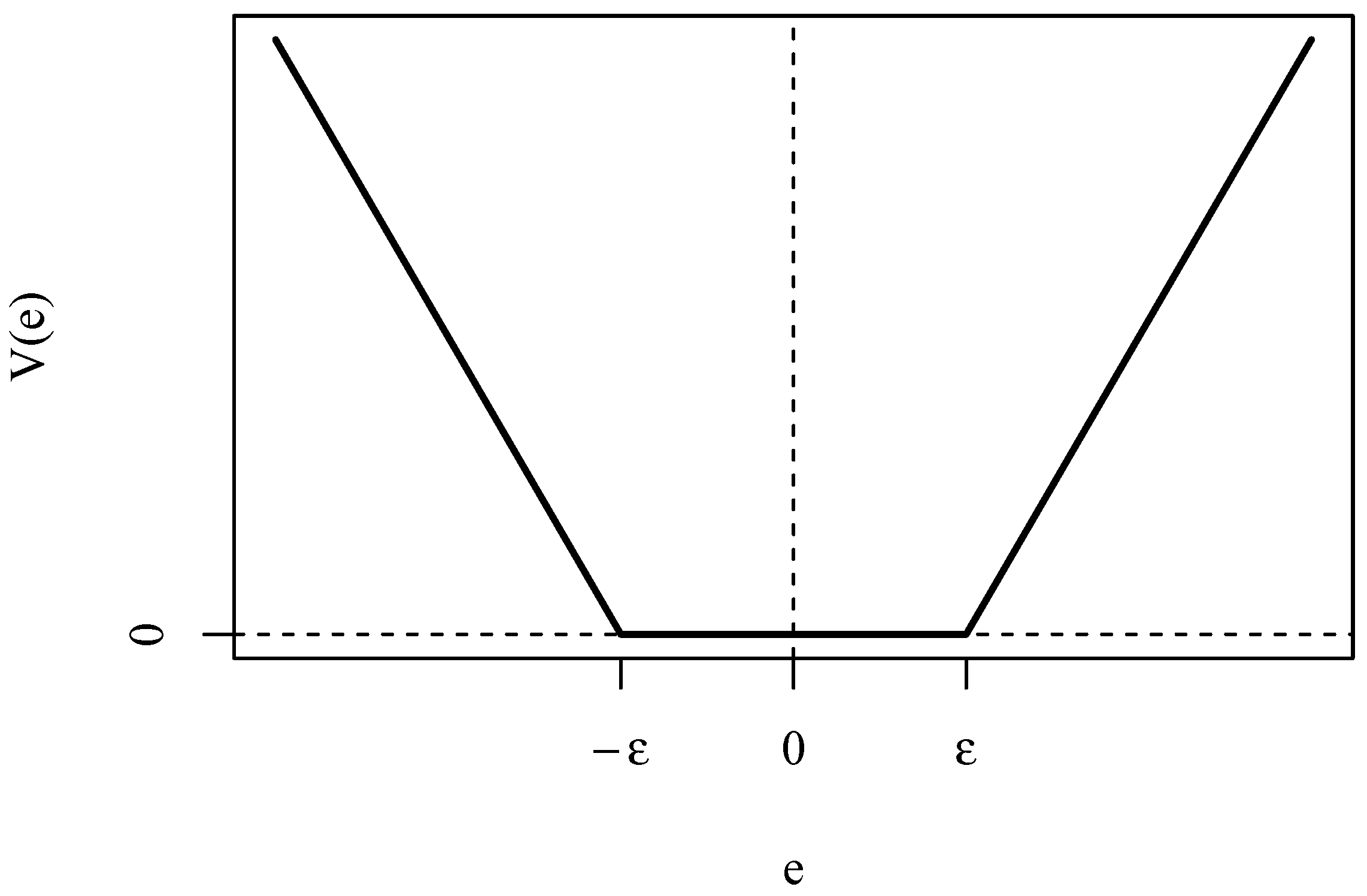
Support vector machines (SVM) are machine learning models born for classification [24] and then adapted to regression [25,26,27]. The regularized loss function for SVM is

$$\sum _{t=p+1}^T{V}_{ϵ}(y_t-f\left(x_t\right))+\frac{\lambda }{2}{\left|\right|\beta \left|\right|}_2^2,$$

with loss

$$V_{ϵ}\left(e\right)=\left\{\begin{array}{cc}0\hfill & \mathrm{if}\left|e\right|<ϵ\hfill \\ \left|e\right|-ϵ\hfill & \mathrm{otherwise}.\hfill \end{array}\right.$$

shown in Figure 1.

When $f(·)$ is linear, it can be shown that the regressors $x_i$ enter the solution of the minimization only through the inner products $\langle x_i,x_j\rangle =x_i^{\top }{x}_j$ and this allows the use of the so-called kernel trick for expanding the class of functions that approximate $f(·)$. Indeed, we can approximate the unknown expectation function using a basis expansion:

$$f\left(x\right)\approx \sum _{s=1}^S{\beta }_s{h}_s\left(x\right)+{\beta }_0,$$

where $h_s(·)$ are basis functions and S is the number of basis functions used to approximate $f(·)$. Since only inner products are relevant for the solution, one does not need to explicitly compute this expansion, but one can simply substitute the inner products with the kernel function $k(x_i,x_j)={\sum }_{s=1}^S{h}_s\left(x_i\right)h_s\left(x_j\right).$

In our application we used the radial-basis function:

$$k(x_i,x_j)=exp\left(-\gamma \left|\right|x_i-x_j{\left|\right|}_2^2\right).$$

Since this expansion through basis functions introduces interactions among the regressors, we expect SVM to be able to capture the mutual dependence of the within-week and within-year seasonal patterns.

The last model considered is the Random Forests (RF; Breiman, 2001). It follows a non-linear approach to the forecasting problem and it originated outside the time series ambit, so it is necessary to motivate its application in this context. RF is a modification of the bootstrap aggregation procedure called bagging introduced by [28]. Bagging belongs to the family of ensemble learning models and consists in producing a number B of bootstrap samples from the available observed sample, estimating a model, called base learner, on each bootstrap sample and then aggregating their predictions. Ordinary bootstrap is suitable for independent and equally distributed observations, so not for time series. Nevertheless, in the case of time series, one assumes that all of the memory of the past regarding $y_t$, required for a one-step-ahead prediction, is preserved in the lagged vectors ${\mathbf{r}}_{t-1}$, so under this assumption the units to be sampled are not the single $y_t$ (with the related exogenous), but the rows of the matrix $\mathbf{D}$. Alternatively, limited to the submatrix $\mathbf{Y}$ of $\mathbf{D}$, resampling the rows of $\mathbf{Y}$ can be viewed as applying the moving block bootstrap [29], where the block length is equal to $p+1$ and the overlapping blocks are the vectors $[y_t,{\mathbf{r}}_{t-1}]$. Ref. [30] have explored the applicability of bagging for time series forecasting. The base learner used in RF is the regression tree, which is the specification of a decision tree when the target variable is continuous. A decision tree [31] is a machine learning model that recursively partitions the data space generated by k explanatory variables into regions, identified by the leaf nodes of the tree, that are homogeneous with respect to a target variable, and fits a simple model in each region. To identify these regions, the splitting and pruning activity is evaluated using a measure of node impurity. The application of this kind of model for time series forecasting is not new in literature; for example, Ref. [32] compared the predictive power of eight machine learning models, including the regression tree, whereas [33] studied the empirical forecast performances of boosting algorithms for predicting real world time series considering as base models the regression tree and the multilayer perceptron. As said before, RF is a modification of the bagging algorithm with a decision tree as base learner, introducing a random selection of input features which causes a collection of de-correlated trees. In fact, if in bagging method the sampling is completed considering instances from only the training set, with random forest the tree-growing process is performed also through random selection of input variables. The parameters involved in a RF specification are the number of trees forming the forest ($N_T$), the number of covariates that are randomly selected at each split step ($mtry$) and the minimum number of observations presented into a leaf node ($nodesize$). When the target variable is continuous, a typical choice for $mtry$ is $\lfloor k/3\rfloor$, where k is the number of the considered explanatory variables, whereas 5 is the choice for $nodesize$.

Variable Importance Measures

When using RF, the well interpretable structure of the tree is lost, but it is possible to retrieve some information regarding the explicative role played by the regressors via variable importance measure (VIM). A VIM is a tool that can be computed not only in the context of the RF. In fact, we can distinguish between two types of methods, when dealing with VIM, that is model-specific and model-agnostic methods [34]. The model-specific methods use specific elements of the structure of the considered model whereas the model-agnostic methods do not assume anything about the structure of the considered model.

The method described below, applied in the RF context, belongs to the first type of methods. Following [31], let $\{X_1,X_2,\dots ,X_k\}$ be the set of predictor variables for the target variable Y, the importance of a variable $X_j\in \{X_1,X_2,\dots ,X_k\}$ in explaining Y is defined as the total decrease in heterogeneity of Y given the by the knowledge of $\{X_1,X_2,\dots ,X_k\}$ when the regressors’ space is partitioned recursively. A VIM, called Total Decrease in Node Impurity (TDNI), derived by this approach is obtained by the sum of all the decreases in the heterogeneity index in the nodes of the tree. Given the different nature of the variables forming $\{X_1,X_2,\dots ,X_k\}$ in many contexts of application, we need to ask if the nature of a regressor plays a role in the evaluation of its importance. Ref. [31] noted that the TDNI measures tend to favor covariates with more values (for example continuous variables are favored over categorical variables), so a correction that overcome this limit must be applied. In this study, the heuristic correction proposed by [35,36] was implemented, given that the set of covariates was composed by continuous, dichotomous and polytomous category variables. Ref. [36] have shown that this method can effectively reduce the bias due to different measurement levels of the covariates, producing a correct ranking of them according to their importance.

In order to investigate the influence of the predictor variables on the electricity price predicted by the other methods implemented in the paper, we use a model-agnostic method based on permutations [34]. It is based on the loss function $\mathcal{L}(\widehat{\mathbf{y}},\mathbf{X},\mathbf{y})$ which quantifies the goodness of fit of the model in use, where $\mathbf{X}$ denotes the matrix containing the observed values of the covariates, $\mathbf{y}$ denotes the observed values of Y and $\widehat{\mathbf{y}}$ denotes the corresponding predictions.

This loss function can be the value of log-likelihood or any other model performance measure, such as, for example, the root mean squared error. The method can summarized in the following steps: compute the loss function for the original data ${\mathcal{L}}^0$ and then, for each regressor $X_j$, (1) modify the matrix $\mathbf{X}$ by permuting its j-th column, obtaining ${\mathbf{X}}^j$; (2) compute the predictions ${\widehat{\mathbf{y}}}^j$ based on ${\mathbf{X}}^j$; (3) calculate the loss function ${\mathcal{L}}^j$; and (4) quantify the importance of $X_j$ using directly ${\mathcal{L}}^j$ or calculating $vi{m}_D^j={\mathcal{L}}^j-{\mathcal{L}}^0$ or $vi{m}_R^j={\mathcal{L}}^j/{\mathcal{L}}^0$. In general, this procedure is performed several times, in order to lose the dependency of the result to the particular permutations observed, and so the final VIM is an average VIM.

As it is well known, decision and regression trees model interactions through different paths of partitions of the feature space: the variables and values selected at lower layers of the trees depend on the variables and values selected in upper layers. Of course, RF is an ensemble of decision trees. Support vector machines/regressions produce interactions among variables by using bivariate kernels, that is, by building a new feature space that includes these non-linear functions of every variable pair. Thus, both methods automatically include interactions among variables. However, being black-box models, it is not straightforward to disentangle the direct effect of one variable from its effect through interactions with other variables. It is important to stress that the variable importance method used in this paper to assess the predictive power of each regressor, measures the effect produced by excluding one variable from the model. In principle, it is possible to think of methods to evaluate the importance of the interactions, even though, to the best of our knowledge nobody did it. For example, to measure the interactions among the variables $X_1,X_2,X_3$ we could use the difference between the loss in RMSE when randomly permuting all of them and the sum of the RMSE losses due to the permutation of each of three variables taken one at a time. However, the number of measures to consider would be extremely large because all variables potentially interact. Consider the extremely simple case of four regressors: $X_1,X_2,X_3,$ and $X_4$. We would have to measure the interactions among:

• Every unique pair $(X_i,X_j)$,
• Every unique triplet $(X_i,X_j,X_k)$,
• All variables $(X_1,X_2,X_3,X_4)$.

This amounts to 11 measures of interaction. For m variables, the number of interactions to consider is $2^{(m-1)}$. In our model, we consider tens of variables and the number of interaction measures to consider are in the order of millions.

3. Empirical Analysis

The time series used in the present work concern the electricity prices from the Italian Power Exchange (IPEX) market. They cover the period from 1 January 2015 to 31 August 2019; the eight months of 2019 were left out for out-of-sample forecasting. The data have an hourly frequency; therefore, each day consists of 24 load periods, with 00:00–01:00 a.m. defined as period 1. Spot price is denoted as $P_{tj}$, where t specifies the day and j the load period, $t=1,2,\dots ,N;j=1,2,\dots ,24$.

The Italian electricity market is divided into different zones, which were the following six until 31 December 2020: North (NOR), Centre-North (CNOR), Centre-South (CSOU), South (SOU), Sicily (SIC), and Sardinia (SAR). In the map displayed in Figure 2, the six physical zones of the Italian market are shown. The map holds just until the end of 2020, while from January 2021 the geographical structure of the market has been modified: one region of the Centre-North zone has been moved to the Centre-South macro-region and a new macro-zone has been introduced, formed by just one region, Calabria, which has been separated from the South macro-zone. Considering that electricity prices and demand have been strongly affected by the COVID-19 outbreak and the structural change of the zonal market in 2021, the choice to stop the data collection in 2019 is highly motivated. It is important to bear in mind that, usually, auctions are made by considering all bids and offers made by market operators at national level. The final unique national price is set by the intersection of the aggregated national supply and demand curves. Inefficiency of the interconnections among zones, which can be observed on the map, implies however a market splitting in two or more macro-zones with different equilibrium prices fixed by the intersections between aggregated partial demand and supply curves. For this reason, time series of zonal prices are often studied and modeled separately. Different probabilities of congestion events between macro-zones and different generation mix can be observed in the Italian macro-zones: this motivates separate estimated models for each zone.

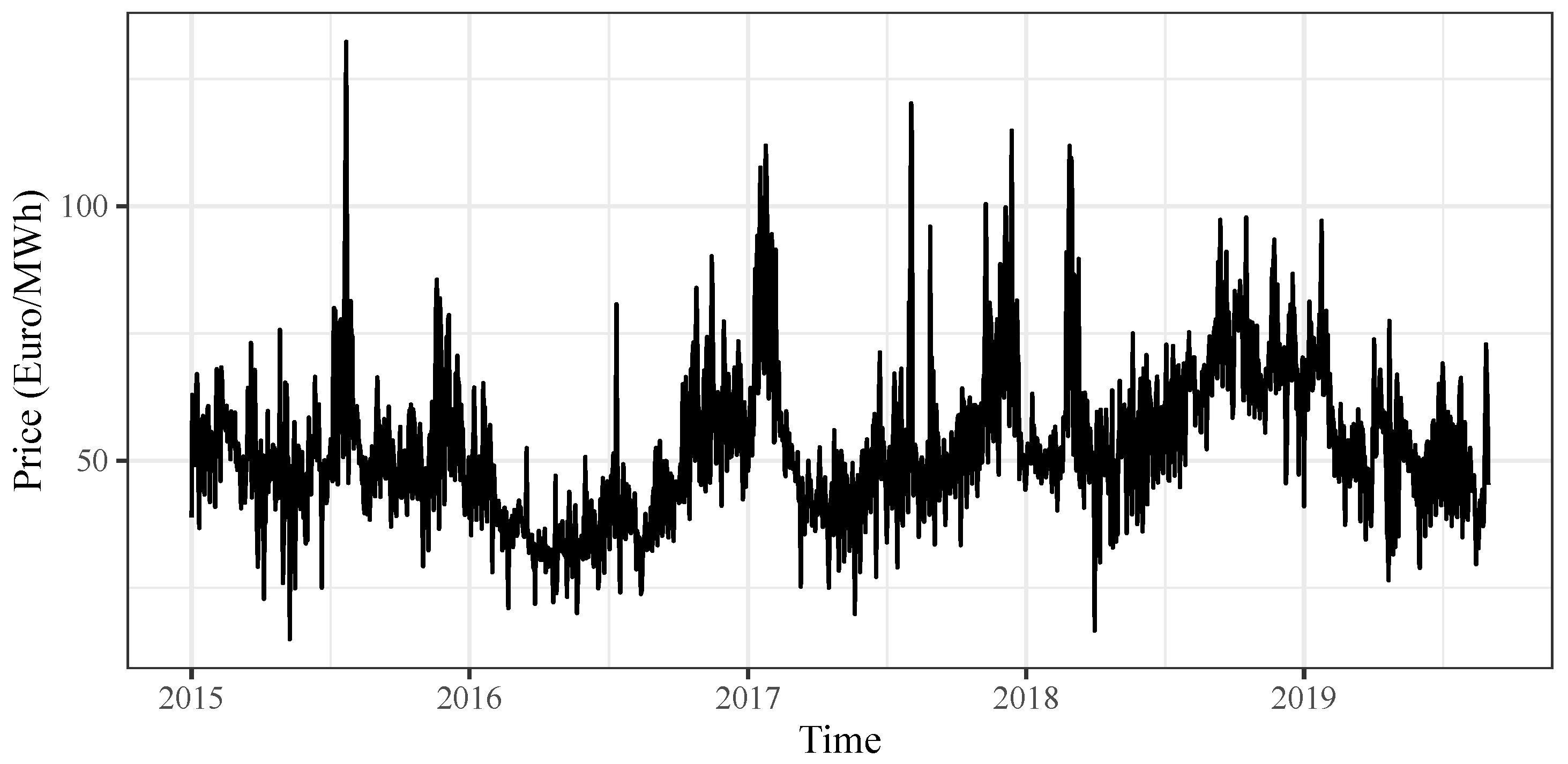
In this study, following a widespread practice in literature, each hourly time series was modeled separately, thereby eliminating the problem of modeling intra-daily periodicity. Moreover, each zone was considered separately. Figure 3 shows the time series of prices in a typical peak hour (12 a.m.) observed in the North zone.

Some stylized facts of electricity prices can be observed, such as the seasonal pattern related to astronomical seasons and the presence of a few spikes. It is worth stressing that multi-scale seasonality is observed on electricity prices: besides yearly fluctuations, weekly, and daily cycles are observed strictly related to the cycles of demand. Several sources of price spikes can be mentioned. They are always related to a sudden increase or decrease in demand and supply of electricity which can be caused by extreme weather events (very hot or cold days) or by plant failures. Of course, parameter estimates can be strongly influenced by the presence of spikes and robust methods should be applied [5].

Table 1. Phillips–Perron unit root test with constant and trend. The test statistics are shown for each hour and zone. The 99% critical value is −3.968721.

Hour	NOR	CNOR	CSOU	SOU	SIC	SAR
1	−10.81	−14.08	−16.01	−17.00	−18.30	−16.41
2	−10.98	−14.42	−16.93	−17.74	−21.71	−17.41
3	−11.32	−14.32	−17.22	−18.24	−22.64	−17.87
4	−12.27	−15.29	−17.80	−18.95	−22.62	−18.45
5	−13.21	−15.93	−18.25	−19.23	−22.15	−18.90
6	−12.82	−15.50	−17.80	−18.56	−23.26	−18.35
7	−14.48	−16.47	−16.82	−17.78	−23.49	−16.92
8	−16.82	−18.92	−19.31	−19.72	−25.57	−19.02
9	−18.81	−20.52	−21.55	−23.18	−25.68	−21.34
10	−18.14	−19.15	−21.59	−23.08	−23.96	−21.52
11	−16.97	−18.42	−20.91	−22.79	−23.76	−21.13
12	−16.77	−18.19	−20.84	−22.24	−23.60	−20.87
13	−15.18	−16.34	−18.72	−21.36	−23.44	−19.56
14	−15.98	−17.57	−19.26	−21.13	−22.57	−20.37
15	−18.66	−20.08	−21.59	−22.30	−23.18	−22.35
16	−18.24	−19.38	−19.39	−21.70	−23.35	−20.95
17	−17.29	−17.58	−17.50	−19.38	−22.76	−18.97
18	−13.48	−13.75	−13.98	−15.86	−19.99	−14.55
19	−12.62	−13.14	−14.26	−15.94	−23.09	−14.50
20	−13.61	−15.99	−17.15	−18.15	−22.89	−17.23
21	−13.39	−20.31	−20.87	−22.13	−23.59	−21.41
22	−12.96	−19.07	−19.17	−20.45	−23.56	−20.26
23	−10.49	−13.72	−14.03	−14.71	−18.64	−15.39
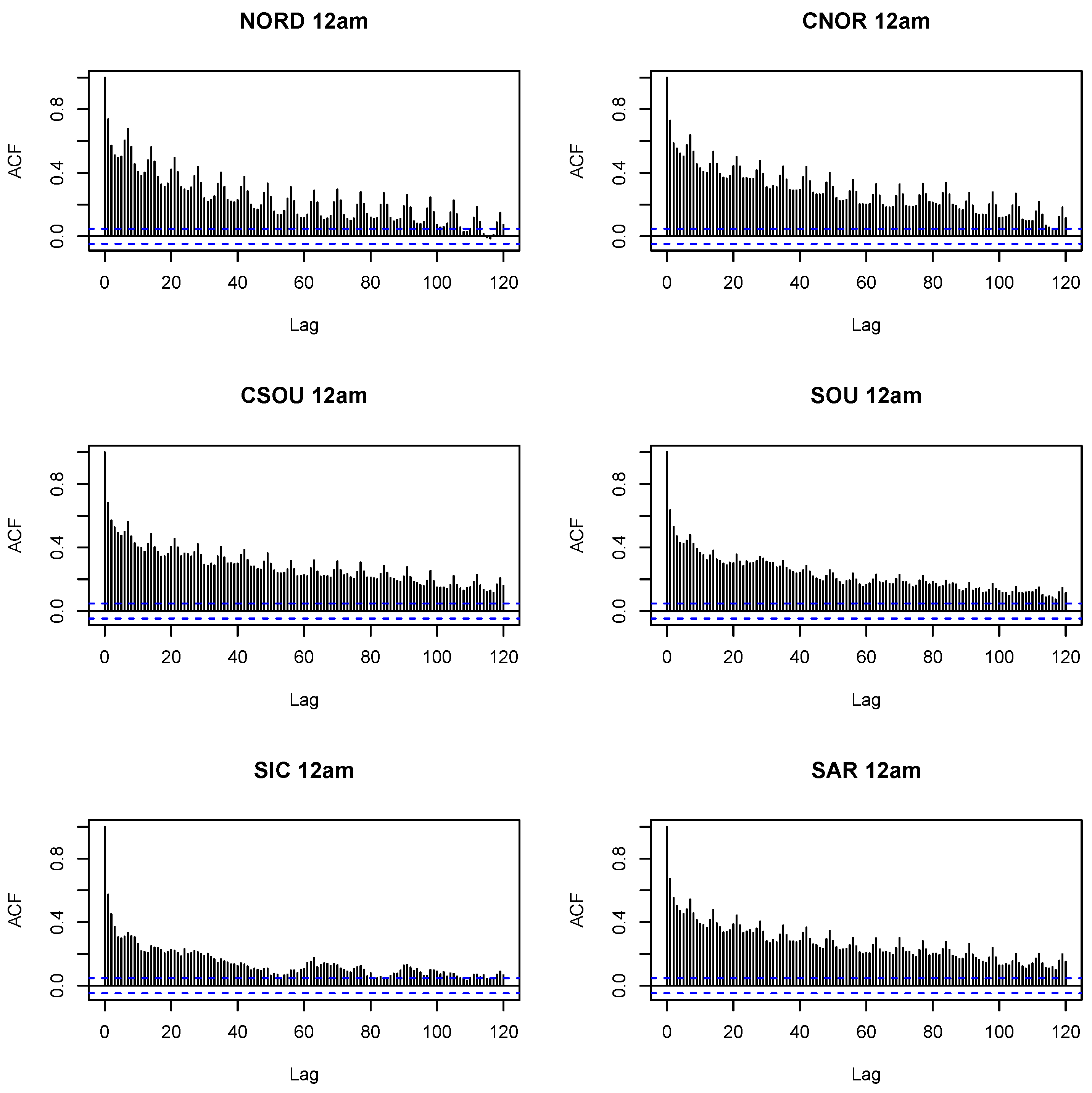
24	−9.24	−11.37	−11.61	−12.83	−15.66	−12.52

shows the unit root test (Phillips–Perron), for each zone of the market and for all settlement periods of the day. Figure 4 displays the autocorrelation function until lag 120 of the level of prices observed in each zone in the middle of the day. Plots in each hour of the day are very similar and are not shown for lack of space. The test always rejects the presence of a unit root, while from the ACF plots weekly seasonality is evident. This seasonality is captured in the RF specification by the number-of-day variable, and by harmonics in the other models. Models could be estimated on first differences to check for robustness. However, as the results on unit root are very clear, we decided to avoid this analysis, to stay focused on the main goal of the paper.

Many authors indicate mean reversion (see, for instance, [10,12]) as a typical feature of electricity price time series because unit root test tend to reject the null of integration. This is hard to believe because gas prices are well described by integrated processes and electricity prices depend also on gas prices (at the time of writing, the relation between gas and electricity prices is extremely evident!). The reason for the rejection of unit root tests is that the signal (with unit root) is generally buried in a high-variance noise (multi-scale seasonality, relation to weather conditions, strategies of the companies playing in the market, plant outages, lines congestions, etc.). So why are we modelling levels and not increments?

• We provide regressors that, in case of unit roots, are certainly cointegrated with the outcome variable, namely the intermediate markets. Regressions with cointegrated variables are valid.
• We are interested in short-term forecasts and for this case even the eventual attraction of a stationary model prediction towards the marginal mean of the time series is generally negligible.
• The range of the time series tends to be constant throughout the time and this enables the use of tree-based models (such as RF), which produce predictions only in the range observed in the training set.

In this study, we integrate the information given by the price at time $t-1,\dots ,t-7$, labelled as y1, y2, …, y7, with a set of deterministic and exogenous regressors (see [1,37]) listed below, in order to improve the capability of the models in hand to predict the future: Data can be downloaded, upon request (luigi.grossi@unipd.it), at the following link: https://drive.google.com/drive/folders/1N-seSvGxQ7hzhocO4hm4WJpxzai1BVqV?usp=share_link (Last update: 30 November 2022).

• The day of the year (day),
• The day of the week (dayweek), a categorical variable with seven classes,
• A calendar dummy for holidays (calendar),
• The one-day-ahead predicted demand of electricity (demand, source: Italian Electricity Market Manager, GME),
• The one-day-ahead predicted wind generation (wind, source: TERNA SpA),
• Four Intra-Day Market (IDM) prices at time $t-1$.

The day of the year is a discrete variable with values from 1 to 366 counting the day number since 1st January of every year. It is used only for the RF, whereas it is replaced by sinusoids at the first 16 harmonics with base period 365 for all the other models. In other words, the following 32 regressors are added to the models: $cos\left({\omega }_{j}t\right)$, $sin\left({\omega }_{j}t\right)$ with ${\omega }_j=2\pi j/365$ and $j=1,2,\dots ,16$.

The reason for this choice relies on the following motivation. Since RF are based on trees, which approximate smooth functions with steps, we provide the RF regression with information on the within-year seasonal periodicity through a variable counting the number of days since the beginning of each year letting the trees find the differences in the sub-periods. Instead, for linear models, such as ARX and ARX-L, or models, such as SVM, that take smooth transforms of the regressors, we provide information on the within-year seasonal periodicity through low-frequency sinusoids. The choice of the number of harmonics (16) is based on the authors’ experience working with Italian price data: the number of harmonics used for other countries is generally much smaller, but the typical drop in electricity consumption (and, thus, prices) on Winter and Summer holidays in Italy requires more sinusoids to be well captured.

Differently from what has been completed so far in the literature, we explore the role played by prices observed on Intra-Day Market (IDM). The IDM allows market participants to modify the schedules defined in the Day-Ahead Market by submitting additional supply offer or demand bids and is organized in seven sessions. Nevertheless, in this study we consider only the first four (IDM1, IDM2, IDM3, and IDM4) with the following timing: IDM1 opens at 12.55 p.m. of the day before the day of delivery and closes at 3 p.m. of the same day (its results are made known within 3.30 p.m. of the day before the day of delivery); IDM2 opens at 12.55 p.m. of the day before the day of delivery and closes at 4.30 p.m. of the same day (its results are made known within 5 p.m. of the day before the day of delivery); IDM3 opens at 5.30 p.m. of the day before the day of delivery and closes at 11.45 p.m. of the same day (its results are made known within 00.15 p.m. of the day of delivery); and IDM4 opens at 5.30 p.m. of the day before the day of delivery and closes at 3.45 a.m. of the day of delivery (its results are made known within 4.15 a.m. of the day of closing of the sitting). Given the different schedule of the sessions, the four regressors related to the IDM market are not all available for all the 24 h.

As seen in Section 2, the methods under study depend on some hyper-parameters and their tuning is performed as follows. For the ARX-L and ARX-L Int. the hyper-parameter for $L_1$ penalization, $\lambda$, is fixed zone by zone and hour by hour by 10-fold cross-validation. For SVM, we use a radial kernel function with $ϵ$ and $\gamma$ determined by 10-fold cross-validation on a grid of $3\times 7$ predetermined values, whereas for RF, $mtry$ and $nodesize$ are set equal to the typical choices, and $N_T=$ 10,000.

We calculate the one-day ahead prediction using a rolling window procedure for the eight months of 2019 and the forecasting performance is evaluated by means of a modified version of the Root Mean Squared Percentage Error (RMSPE) and the Mean Absolute Percentage Error (MAPE).

Two simple benchmarks have been introduced. The first is the Random Walk (RW), under the trivial hypothesis that the price observed in t could be predicted by the price observed in $t-1$ (naive model). Comparisons of the estimated models to the RW are shown in

Table 2. Comparison of forecasting performances to those of the RW model over peak (14 h) and off-peak (10 h) hours. Values are obtained as the ratio of the model’s average RMSE to the average RMSE under the Random Walk assumption, over the prediction horizon in the same hour group (peak and off-peak).

	Area	ARX	ARX-L	ARX-L Int.	RF	SVM
Peak hours	NOR	0.706	0.735	0.727	0.736	0.702
	CNOR	0.727	0.744	0.740	0.766	0.731
	CSOU	0.756	0.774	0.774	0.780	0.766
	SOU	0.775	0.803	0.795	0.793	0.785
	SIC	0.833	0.861	0.862	0.847	0.850
	SAR	0.776	0.786	0.782	0.787	0.777
Off-peak hours	NOR	0.779	0.814	0.802	0.807	0.787
	CNOR	0.803	0.822	0.822	0.826	0.815
	CSOU	0.841	0.848	0.856	0.843	0.845
	SOU	0.824	0.835	0.844	0.830	0.831
	SIC	0.846	0.866	0.859	0.845	0.851
	SAR	0.846	0.848	0.861	0.835	0.841

. The second benchmark is the “naive week” RW, under the hypothesis that the daily price in t could be predicted by the price in $t-7$ (same day of the previous week). Results are displayed in

Table A1. Comparison of forecasting performances to those of the “Naive Week” RW model over peak (14 h) and off-peak (10 h) hours. Values are obtained as the ratio of the model’s average RMSE to the average RMSE under the “Naive Week” assumption, over the prediction horizon in the same hour group (peak and off-peak).

	Area	ARX	ARX-L	ARX-L Int.	RF	SVM
Peak hours	NOR	0.701	0.729	0.721	0.730	0.696
	CNOR	0.697	0.713	0.709	0.735	0.701
	CSOU	0.710	0.728	0.727	0.733	0.720
	SOU	0.713	0.738	0.731	0.729	0.722
	SIC	0.707	0.731	0.732	0.719	0.722
	SAR	0.722	0.731	0.728	0.732	0.723
Off-peak hours	NOR	0.674	0.704	0.694	0.698	0.681
	CNOR	0.686	0.702	0.702	0.705	0.696
	CSOU	0.697	0.702	0.709	0.698	0.700
	SOU	0.705	0.714	0.722	0.710	0.711
	SIC	0.674	0.689	0.684	0.673	0.677
	SAR	0.708	0.709	0.720	0.698	0.704

. Adjustment for holidays has been considered. As can be noted, all values are less than 1, proving that all models perform better than the corresponding naive model.

Moreover, the significance of prediction differences between models is evaluated with the one-tailed Diebold–Mariano test [38], with the null hypothesis declared as “prediction performance of model A is equal or worse than model B”. Nevertheless, in what follows, we show and discuss only the results obtained applying RMSPE, given that the same conclusions arise from the MAPE analysis. MAPE values are shown in

Table A2. Mean value of MAPE over peak (14 h) and off-peak (10 h) hours. Values are obtained as the percentage ratio of MAE to the average price observed over the prediction horizon in the same hour group (peak and off-peak).

	Area	ARX	ARX-L	ARX-L Int.	RF	SVM
Peak hours	NOR	9.02	9.29	9.15	9.16	8.78
	CNOR	9.09	9.22	9.13	9.42	8.97
	CSOU	9.83	10.06	10.04	10.12	9.88
	SOU	13.51	14.29	14.19	13.85	13.86
	SIC	22.47	23.76	23.67	23.14	23.20
	SAR	10.90	11.07	11.03	11.08	10.95
Off-peak hours	NOR	8.32	8.63	8.51	8.51	8.33
	CNOR	8.82	9.01	8.99	9.02	8.92
	CSOU	10.46	10.63	10.75	10.58	10.59
	SOU	11.03	11.29	11.47	11.22	11.22
	SIC	17.47	18.15	17.96	17.56	17.69
	SAR	11.02	10.93	11.12	10.81	10.94

.

Table 3. Mean value of RMSPE over peak (14 h) and off-peak (10 h) hours. Values are obtained as the percentage ratio of RMSE to the average price observed over the prediction horizon in the same hour group (peak and off-peak).

	Area	ARX	ARX-L	ARX-L Int.	RF	SVM
Peak hours	NOR	12.12	12.62	12.47	12.63	12.05
	CNOR	12.28	12.57	12.50	12.94	12.35
	CSOU	13.42	13.74	13.73	13.85	13.60
	SOU	18.69	19.36	19.18	19.12	18.92
	SIC	30.85	31.91	31.95	31.38	31.51
	SAR	15.75	15.96	15.88	15.98	15.78
Off-peak hours	NOR	10.84	11.33	11.16	11.22	10.96
	CNOR	11.80	12.08	12.07	12.13	11.98
	CSOU	14.17	14.28	14.42	14.20	14.24
	SOU	15.14	15.33	15.51	15.24	15.27
	SIC	24.02	24.58	24.39	23.99	24.15
	SAR	14.69	14.72	14.94	14.50	14.61

contains the ratio of the mean value of RMSE over peak (14 h) and off-peak (10 h) hours over the corresponding average price. For instance in Table 3, the value in the first line, first column, is obtained as the ratio of the RMSEs generated by ARX model in each of the 14 peak hours in the NOR zone, over the average price observed on the forecasting horizon in the NOR zone. This generalized version of the RMSPE is better than the proper RMSPE because it avoids the bias related to cases in which prices close to zero generate very large ratios. It is of interest to distinguish between these two types of hours because companies adopt different strategies when demand is high or low. All the models perform better during the off-peak hours, since when demand is low the supply curve is rather flat and the elasticity of the price rather low (i.e., unexpected changes in demand have a small effect on the equilibrium price). Moreover, the predictive performances seems equivalent for the North and the Center-North of Italy, whereas they become worse moving from the North to the South and islands. Electricity prices for Sicily appear quite difficult to accurately predict due to the frequent and scarcely predictable switch between two regimes: as a separate market with a higher price and as part of the Italian market with a common (lower) price. Looking at the values of the RMSPE, in the peak hours SVM seems to outperform the other models in the North whereas the ARX seems to show better predictive capacities in the remaining areas. In the off-peak hours ARX seems to outperform the other models in all the areas except for Sicily and Sardinia where RF seems to predict slightly better the spot prices.

In order to inspect more deeply the predictive performances of the models, the performances on the single hours were considered.

Table 4. Best model according to minimum RMSE—peak and off-peak hours.

PEAK HOURS
Hour	NOR	CNOR	CSOU	SOU	SIC	SAR
8	SVM (2)	ARX (2)	ARX (1)	ARX (1)	ARX (3)	ARX (1)
9	ARX (2)	ARX (2)	ARX (0)	ARX (2)	ARX (2)	ARX (0)
10	ARX (3)	ARX (1)	ARX (1)	ARX (2)	RF (0)	ARX (0)
11	SVM (1)	ARX (0)	ARX (0)	ARX (1)	ARX (2)	RF (0)
12	SVM (3)	ARX (0)	ARX (0)	RF (0)	ARX (2)	ARX (0)
13	SVM (3)	ARX (1)	ARX (0)	RF (0)	ARX (1)	RF (0)
14	SVM (2)	ARX (0)	ARX (0)	ARX (0)	ARX (2)	ARX (0)
15	SVM (1)	ARX (1)	ARX (0)	ARX (0)	ARX (1)	ARX (1)
16	ARX (0)	ARX (1)	ARX (1)	ARX (1)	ARX (2)	ARX (3)
17	SVM (1)	ARX (0)	ARX (3)	ARX (4)	ARX (2)	ARX (3)
18	ARX (1)	ARX (1)	ARX (3)	ARX (4)	ARX (3)	ARX (2)
19	SVM (1)	ARX-L Int. (0)	SVM (1)	ARX (4)	RF (3)	SVM (0)
20	SVM (0)	ARX-L (0)	ARX-L (2)	ARX (1)	ARX (4)	ARX-L Int. (2)
21	SVM (1)	ARX-L Int. (1)	ARX-L (2)	ARX-L (0)	ARX (3)	RF (1)
OFF-PEAK HOURS
Hour	NOR	CNOR	CSOU	SOU	SIC	SAR
1	ARX (3)	ARX (3)	ARX (2)	ARX (3)	SVM (0)	ARX (1)
2	ARX (3)	ARX (4)	ARX (2)	ARX (3)	ARX (0)	ARX (2)
3	ARX (4)	ARX (4)	RF (1)	RF (1)	ARX-L Int. (0)	RF (1)
4	ARX (4)	ARX (3)	ARX (3)	ARX (2)	RF (0)	RF (1)
5	ARX (4)	ARX (4)	ARX (3)	ARX (3)	RF (0)	RF (0)
6	ARX (2)	ARX (4)	RF (0)	RF (0)	ARX-L Int. (0)	RF (0)
7	ARX (3)	ARX (3)	ARX (1)	ARX (0)	ARX (3)	ARX (0)
22	RF (0)	SVM (1)	ARX-L Int. (0)	RF (0)	RF (2)	ARX-L (1)
23	SVM (0)	SVM (1)	SVM (0)	SVM (0)	ARX (0)	RF (2)
24	RF (2)	ARX (0)	ARX-L (0)	ARX-L (0)	RF (0)	SVM (1)

displays, for each hour, the model with the lowest RMSE and in brackets the number of significant Diebold and Mariano tests. This number ranges between 0 and 4, with 0 meaning that the RMSE of the best model is not significantly lower than the RMSE of the other 4 competitors, and 4 meaning that the RMSE of the best model is always significantly lower. For most of the hours the ARX has the lowest RMSE in all the areas, with the exception of North and peak hours, where the SVM outperforms for most of the hours, and Sicily, Sardinia, and off-peak hours, where RF outperforms for most of the hours. Nevertheless, in very few cases the number of significant Diebold and Mariano tests reaches 4.

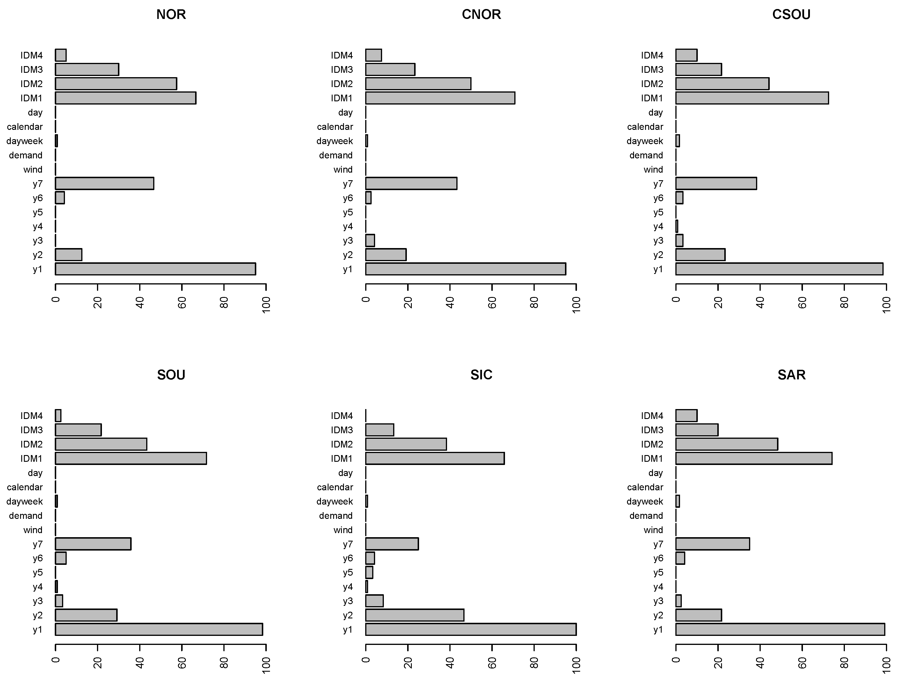
In order to investigate more deeply the observed results, we analyze the role of the used explanatory variables in the models’ performance calculating the VIM for RF, ARX-L, and SVM. The implemented methods are described in Section 2. To summarize the results, we took into account only the covariates that occupy one of the first five positions in the ranking produced by the VIMs. Moreover, with the aim to discriminate the relevance of the ranking, we assign the values reported in

Table 5. Values assigned to the first five positions in the ranking.

Pos. 1	Pos. 2	Pos. 3	Pos. 4	Pos. 5
1	0.8	0.6	0.4	0.2

to the five positions.

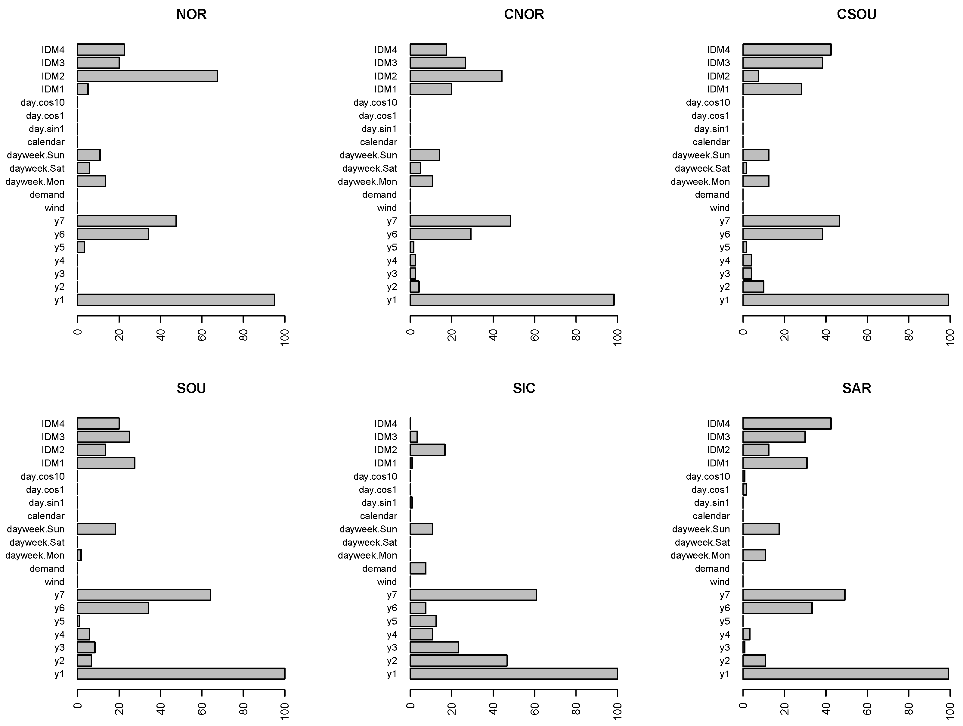
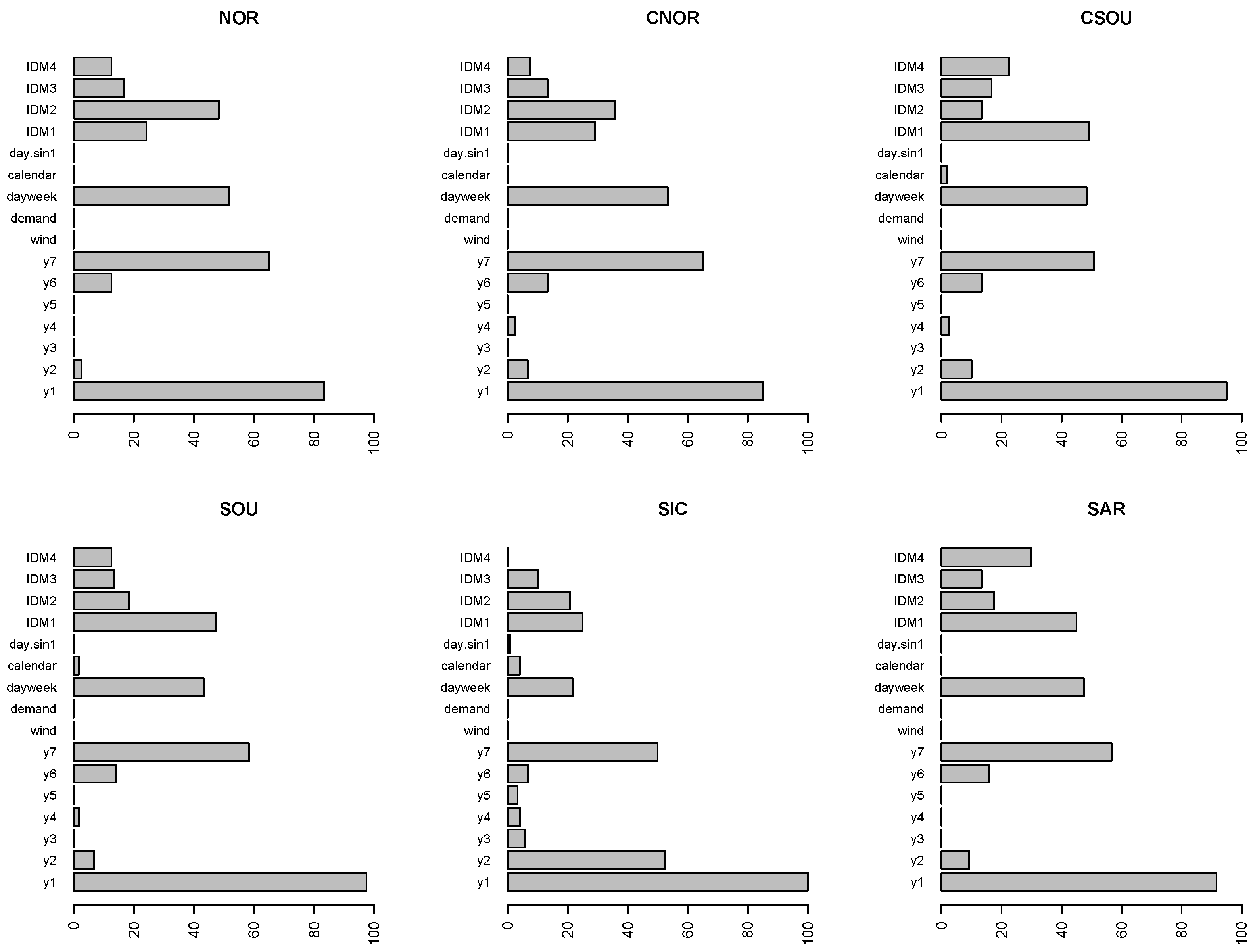
Figure 5, Figure 6 and Figure 7 compare the relevance of regressors obtained in the different zones using the modified version of the variable importance index when RF predictions are evaluated, and using the model-agnostic method based on permutations for the evaluation of forecasts from SVM and ARX-L.

The bars represent the weighted percentage of times the variables are within the fifth position out of the 24 h. To evaluate correctly the results, we have to consider that prices for the last two sessions of the IDM are not available for all the 24 h, so for IDM3 and IDM4 the bars refer to the weighted percentage out the 12 and 8 h, respectively.

For all three models, the lagged spot prices until the seventh lag, and, in particular, the first and the seventh delay, are among the most important variables.

Intraday prices generated across all IDMs are at the top in the VIM rankings, as well. Nevertheless, differences can be spotted comparing the three models. In general, all the IDMs seem less important for both SVM and ARX-L, than for RF.

In the case of RF, the IDM1 and IDM2 are the most important in all the six zones, and the importance of IDM1 is comparable with the first lagged spot price.

When ARX-L is used (Figure 6), the IDM4 plays a predominant role within the IDMs in the Center-South and Sardinia, whereas in North and Centre-North IDM2 is the most important. Differently from the other zones, in Sicily intra-day markets are almost negligible, while the autoregressive structure looks very strong.

Looking at Figure 7 concerning SVM, IDM1 is the most important of the four IDMs in all the zones moving from Centre-South to the islands, whereas in North and Centre-North IDM2 is the most important. Moreover, the day of the week variable plays a relevant role in all zones.

The high relevance of the autoregressive structure of spot prices until the seventh lag is a common feature of all models in all zones. It is sensible to assume that this common feature could be the main explanation of the excellent forecasting performance of linear AR models. To test this assumption, the forecasting exercise has been repeated removing the lagged spot prices from the set of regressors. As pointed out by one of the reviewers, the model obtained by stripping the model from lagged prices is improperly called AR model because a simple regression model on exogenous variables is estimated. However, we prefer to maintain the same label to stress the link with the previous tables. The fitting of the all models without lagged prices is obviously worse. The exercise has been carried out just to measure the different contribution of past information on the prediction using different models. The decrease in the forecasting performance is expected, but the extent of the deterioration is different and gives an idea of the relevance of exogenous variable in various models. We are aware that the exercise has no practical implications. For this reason we do not perform any out-of-sample forecasting test. The comparison between the models with and without the lagged prices is displayed in

Table 6. Percentage variation of average RMSE over peak and off-peak hours with respect to the case in which no lagged values of the dependent variable were included in the regressors set.

	Area	ARX	ARX-L	ARX-L Int.	RF	SVM
Peak hours	NOR	−10.41	−7.00	−8.57	−10.82	−11.47
	CNOR	−12.73	−8.78	−10.17	−10.82	−13.43
	CSOU	−10.62	−9.26	−10.26	−9.13	−11.39
	SOU	−5.68	−5.05	−5.53	−4.36	−6.29
	SIC	−4.62	−9.56	−7.43	−4.23	−5.69
	SAR	−10.90	−7.51	−9.38	−7.70	−10.57
Off-Peak hours	NOR	−14.20	−10.76	−11.03	−11.93	−15.38
	CNOR	−17.20	−14.41	−14.59	−13.43	−16.68
	CSOU	−14.88	−12.87	−11.73	−10.22	−13.79
	SOU	−10.28	−9.84	−8.43	−7.66	−9.40
	SIC	−3.35	−10.30	−11.22	−2.38	−3.67
	SAR	−16.59	−11.39	−11.63	−10.12	−14.90

, which contains the percentage variation of the average RMSE computed on the two versions of the models for each zone, that is:

$$\left(\frac{\mathrm{RMSE}\left(\mathrm{MAE}\right)withpastprices}{\mathrm{RMSE}\left(\mathrm{MAE}\right)withoutpastprices}-1\right)\times 100.$$

All figures in Table 6 are negative, as expected. Similar results have been found for MAE.

Looking at the peak hours, the biggest reduction in predictive capability in all zones except Sicily, occurs for SVM; nevertheless, this reduction is similar to that of ARX models. Therefore, the impact of past prices on the predictions of ARX and SVM models is bigger than in all the other cases.

During the off-peak hours, the ARX models show the highest reduction of predictive capability in all zones, but the North. The case of RF is quite interesting. For this model, the reduction of forecasting ability due to the exclusion of lagged spot prices is lower than for SVM and ARX models in almost all 24 h. The relevant role played by IDMs in RF models seems to replace the contribution of lagged spot prices.

The effect of exogenous covariates on the forecasting performance has been explored as well. In this case, the percentage variation of the average RMSE (MAE) over each zone is computed as follows:

$$\left(\frac{\mathrm{RMSE}\left(\mathrm{MAE}\right)withexogenousvariables}{\mathrm{RMSE}\left(\mathrm{MAE}\right)withoutexogenousvariables}-1\right)\times 100.$$

As expected, the sign of these variations for RMSE (

Table 7. Percentage variation of the mean values of RMSE over peak and off-peak hours with respect to the case in which no exogenous variables were included in the regressors set.

	Area	ARX	ARX-L	ARX-L Int.	RF	SVM
Peak hours	NOR	−15.46	−13.87	−13.33	−8.93	−15.51
	CNOR	−14.19	−13.63	−13.19	−8.22	−13.77
	CSOU	−10.98	−10.12	−9.28	−6.87	−9.48
	SOU	−7.79	−4.45	−4.43	−3.79	−5.97
	SIC	−4.53	−1.72	−1.68	−3.28	−2.68
	SAR	−8.08	−7.52	−7.41	−4.84	−7.68
Off-Peak hours	NOR	−9.69	−5.75	−7.26	−6.16	−8.51
	CNOR	−6.34	−3.80	−4.66	−3.73	−5.05
	CSOU	−3.02	−1.46	−1.67	−1.48	−2.17
	SOU	−3.38	−1.45	−1.62	−1.70	−2.57
	SIC	−1.57	0.67	−0.62	−2.26	−1.92
	SAR	−1.94	−1.20	−0.80	−1.65	−2.21

) is always negative. Similar results have been found for MAE.

During peak hours, RF models show the lowest reduction in predictive power in all zones except Sicily, whereas during off-peak hours and in all zones except Sicily, ARX and SVM models lose more predictive power than other models.

Comparing the last two analyses reported in Table 6 and Table 7, the highest reduction in the predictive power occurs when the exogenous variables are removed, during the peak hours in Northern Italy (NOR+CNOR), for all models but RF. This result stresses the crucial role played by IDMs in forecasting spot prices in an area which covers more than 50% of the total national power generation.

On the contrary, during off-peak hours, for all models and hours, the highest reduction in the predictive power occurs when the lagged spot prices are removed, showing a lower contribution to the predictive accuracy of the exogenous variables with respect to lagged prices. To have an idea about the impact of intra-day prices, the same exercise could have been performed by simply removing the IDM variables. However, as can be seen from the variable importance plots (Figure 5, Figure 6 and Figure 7), the most important variables are always $t-1$ and $t-7$ lags on the day ahead price and the IDM variables. Wind and Demand are never crucial. For this reason, we expect that the exercise will lead to the same results obtained when all exogenous regressors are included.

4. Conclusions

The initial research question motivating this study concerns the potential prevalence of sophisticated non-linear methods, such as SVM and RF models, on the simple linear AR model, taken as the benchmark, in predicting one-day ahead spot price. We found that, when estimated in the macro-zones of the Italian electricity market, there is not a clear dominance of one model and in all hours of the day. SVM regressions seem to outperform the other models in the North zone in peak hours (10 h out of 14). It is worth stressing that North is the most important area of the Italian market as it covers about 50% of the national generation. AR models perform better in the other zones. However, statistical prevalence is hard to be found, suggesting that the simplest model (ARX, that is AR with exogenous variables) in general makes a good job in predicting spot prices. Summarizing the results shown in Table 4, the simple ARX model gives the best prediction in 79% of cases considering peak hours in CNOR and CSOU.

Connected with the initial research question, we have studied the issue of variable selection connected to the forecasting performance of models. In addition to the autoregressive structure of the generating process, we considered some exogenous variables commonly used in the literature and available on the Italian market, that is, predicted demand and wind generation, and intra-daily market prices. To the best of our knowledge, the impact of intra-daily market information on the prediction of spot prices is a new research question, never explored before. The influence of regressors on the forecasting ability of different models has been measured using variable importance measures (VIM), which give a clear idea about the most relevant set of regressors. VIM have been originally developed in the framework of RF, given that the structure of the trees involved in the forest and, consequently, the role of the variables are lost. In this paper, we have extended the VIM analysis to ARX and SVM models by applying a model-agnostic method based on permutations. We have found that, for all models, lagged spot prices up to seven days, and IDMs play a crucial role in the prediction step.

For RF, IDM1 and IDM2 are the most important regressors in all six zones, and the importance of IDM1 is comparable to that of the spot price of the same hour on the previous day. For SVM and ARX models, the importance of IDMs is less evident than for RF, although their role is not negligible. The analysis of the impact of the autoregressive structure of the spot prices on the forecasting ability has revealed that, in Northern Italy and in peak hours, IDMs are a crucial set of information to predict spot prices.

The final message is that, for forecasting electricity prices, variables’ construction and selection (or feature engineering, using machine learning jargon), both in the step of dataset preparation and during model estimation is more important than the use of complex non-linear models. Linear models, combined with penalization criteria, provide good forecasting performances, and have great computational and interpretation advantages.

Further research will be devoted to the study of some theoretical properties of RF for dependent data and to the introduction of additional exogenous variables, such as marginal technologies, weather variables, and fuel prices. The main limit of the paper is that just two machine learning models among the large range of machine learning models proposed in the literature have been considered. Although RF and SVM are massively used in the prediction of time series there are other emerging techniques that would be worth to explore. Among these, we just mention the Gradient Boosting and the Dynamic Trees [39] for online forecasting, which have proven to be very effective in the prediction of electricity prices [40,41]. The comparison with other promising machine learning models will be explored in future papers. A possible integration with robust interval prediction will be also studied.