Article

Vibrations Induced by a Low Dynamic Loading on a Driven Pile: Numerical Prediction and Experimental Validation

by
Aires Colaço
1,*,
Pedro Alves Costa
1,
Cecília Parente
1 and
Ahmed M. Abouelmaty
1,2
1
CONSTRUCT-FEUP, Department of Civil Engineering, Faculty of Engineering, University of Porto, Rua Dr. Roberto Frias s/n, 4200-465 Porto, Portugal
2
Arab Academy for Science, Technology, and Maritime Transportation, College of Engineering and Technology, Giza 3650111, Egypt
*
Author to whom correspondence should be addressed.
Vibration 2022, 5(4), 829-845; https://doi.org/10.3390/vibration5040049
Submission received: 21 September 2022 / Revised: 11 November 2022 / Accepted: 14 November 2022 / Published: 17 November 2022
(This article belongs to the Special Issue Vibrations in Materials Processing Machines)

Abstract

:
The present paper addresses the problem of generating and propagating vibrations induced by low-impact loading on a driven pile. In this context, an experimental test site was selected and characterized, where ground-borne vibrations induced by the application of a low dynamic loading on the pile head were measured using accelerometers placed at the ground surface. At the same time, a new numerical approach, based on a coupled FEM-PML (Finite Element Method-Perfectly Matched Layer) formulation, to model the pile–ground system was presented. A very satisfactory agreement was observed between the experimental data collected in these experiments and the prediction performed by the numerical model. The experimental data can be also used by other authors for the experimental validation of their or other prediction models.

1. Introduction

Ground vibrations have become a major environmental concern in urban areas in recent years. These may arise from different sources, disturb activities and people in the vicinity of the source, and even damage existing equipment or structures. Construction activities can be pointed out as an important source of vibration, in which pile driving activities are a particular concern [1,2,3,4].
Impact pile driving (in general) is recognized as a very useful technique for the installation of deep foundations, presenting some advantages, namely with regard to construction time, industrialization, and the automation of construction procedures, among others. However, during driving activities, it is necessary to be aware of the vibration levels induced at the base of surrounding buildings in order to avoid excessive discomfort for residents and, in extreme scenarios, damage to nearby buildings. Thus, it is extremely important that the level of vibrations can be estimated before pile driving operations begin.
The prediction procedure is a complex process since physical phenomena involve different media with distinct properties and mechanical behaviors: the impact hammer device, pile, ground, and structures. In some cases, the difficulty of predicting the vibration levels limits the applicability of the method, with adverse technical and economic effects. In view of this complexity, the vast majority of studies on ground-borne vibrations induced by impact pile driving are based on empirical approaches [5,6,7,8,9,10,11].
Despite the prevalence of empirical approaches, some numerical methodologies have been proposed in recent years, seeking a deeper understanding of the physical behavior of the problem and a more general prediction approach, not restricted by the specific conditions for which the empirical rules were derived. Some of these advances in numerical modeling of vibrations induced by pile driving should be highlighted, namely the studies performed by Ramshaw et al. [12] and by Khoubani et al. [13] in which an axisymmetric finite element model was adopted for the simulation of the pile–ground system. Infinite elements were used for the treatment of the artificial boundaries. A similar modeling technique was presented by Homayoun Rooz and Hamidi [14], using artificial boundaries based on a constant increase in the soil damping to guarantee that incident waves are not able to return to the analysis domain, i.e., fulfilling Sommerfeld’s condition. With a similar strategy that concerns the treatment of artificial boundaries, Sofiste et al. [15] proposed a very efficient numerical model based on an explicit time-domain approach. A different technique, based on the finite element method–boundary element method (FEM-BEM) coupling, was proposed by Masoumi et al. [16,17] to address the same problem. Taking into account that the strain levels of the soil next to the pile are high, Masoumi et. al. [18] proposed a non-linear coupled FEM-BEM approach for predicting free-field vibrations due to impact and vibratory pile driving. Grizi [19] used the finite element software Plaxis 3D (V22.00) to compute the vibration levels induced by impact pile driving, also considering the non-linear behavior of the soil. In a different application field, it is also possible to reference some offshore pile driving models: [20,21,22,23]. Although the offshore environment adds to the complexity of the problem, the available models are used to predict the coupled system dynamics with the exact same focus: environmental vibrations.
Given the complexity of the problem, the experimental validation of the numerical tools is a fundamental step. Despite its importance, there is a real difficulty in finding well-documented case studies in the available bibliography that allow other authors to validate their models. From this perspective, this work presents an experimental test site developed for this purpose, where the developed experimental tests refer to a low-strain analysis of the waves propagated from a driven pile. At the same time, a new numerical approach for modeling the pile–ground system, developed in the frequency domain, is presented.
In terms of organization, the paper begins by presenting the main features of the numerical model proposed for the simulation of the pile–ground system, assuming a linear behavior of the soil, and the impact hammer model. After the explanation of the numerical modeling approach, the experimental site is presented in Section 3. A detailed description of the main characteristics of the site is presented, focusing on the experiments carried out for the validation of the axisymmetric finite element method–perfectly matched layers (FEM-PML) numerical model, which is present in Section 4. The paper ends with some guidelines on how to expand the proposed model to deal with high strains induced by pile driving operations and the main conclusions.

2. Modeling Approach

2.1. Generalities

The numerical prediction of ground vibrations due to impact pile driving requires the modeling of a complex system. In this context, a sub-structuring approach is proposed, comprising two main modules: (i) the pile–ground system, modeled by an FEM-PML approach in axisymmetric conditions; (ii) a dynamic simulation of the hammer device. Both models are coupled, meeting the compatibility and equilibrium requirements. Figure 1 shows the interaction scheme of the methodology.

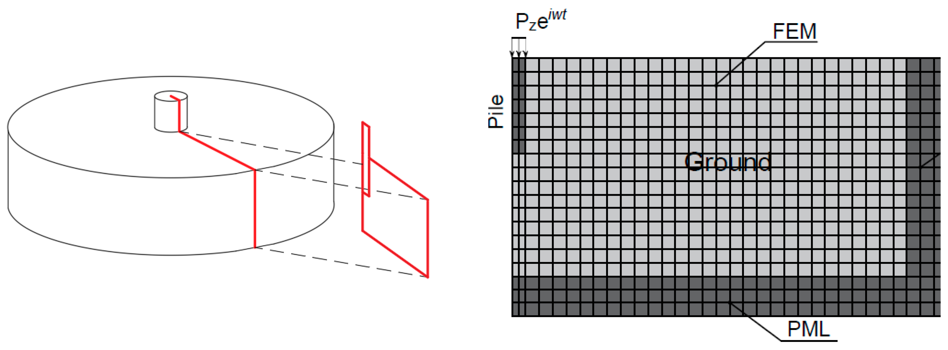
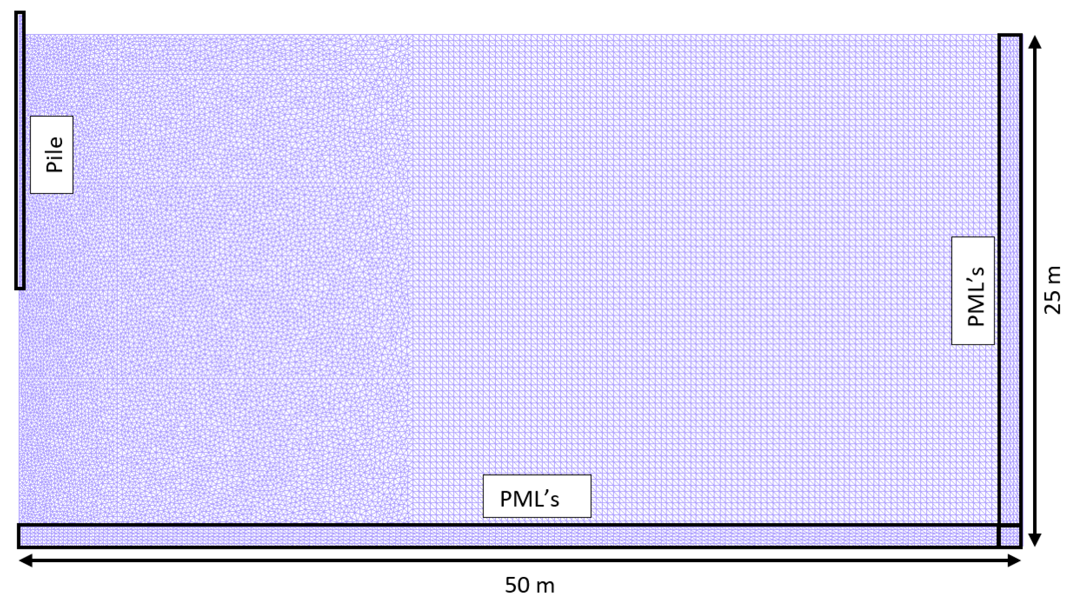
2.2. Axisymmetric FEM-PML Approach: Modeling of the Pile–Ground System

The numerical prediction of free field vibrations due to an impact load on the pile head requires the modeling of the pile and the ground. In the present case, the pile–ground system is modeled through the finite element method and perfectly matched layers in axisymmetric conditions. Perfectly matched layers are used to suppress undesirable spurious reflections of waves in infinite media modeled with finite elements. The modeling approach was implemented in the commercial software MATLAB (V2021b). A schematic illustration of the model is depicted in Figure 2.
According to the principle of virtual work and following the typical steps of the finite element method procedure, the equilibrium equation for any point of a 3D domain can be derived as follows:
V δ ε T σ dV + V δ u T ρ u i x , t t 2 dV = S δ u T pdS
where δ ε is the virtual strain field, σ represents the stress field, δ u is the virtual displacement field ( u is the displacement field), ρ is the volumetric mass, and p represents the external loads applied to the surface S .
For the sake of computational efficiency, an axisymmetric model was assumed for the centerline of the pile, allowing for obtaining a three-dimensional response to the problem without the need for a 3D discretization. Consequently, the integral volume in Equation (1) can be adapted for axisymmetric problems by expressing the differential volume d V as 2 π r d S , where r is the radial distance from the axisymmetric axis. Likewise, the differential surface can be converted to the linear form by expressing d S as 2 π r d L . Converting from the space domain to the frequency domain and introducing the approximation of finite elements, each term of the virtual working condition expressed in Equation (1) can be written as:
2 π S δ ε T σ rdS = 2 π S B T DBu n rdS
2 π S δ u T ρ u i x , t t 2 rdS = 2 π ω 2 S N T ρ Nu n rdS
2 π L δ u T prdL = 2 π L N T prdL
where [ B ] is the strain matrix, [ D ] is the strain-stress matrix, N is the shape function matrix, and u n is the vector of nodal displacements. According to the classic finite elements notation, it follows that
K = 2 π S B T D B r d S
M = 2 π S N T ρ N r d S
where [M] and [K] are the mass and stiffness matrices, respectively.
The stress–strain relation is established by the constitutive matrix D . For an isotropic elastic linear solid, loaded under axisymmetric conditions, this matrix is given by:
D = E * 1 + ν 1 2 ν 1 ν ν ν 0 ν 1 ν ν 0 ν ν 1 ν 0 0 0 0 0.5 ν
where E * is the complex Young modulus and ν is the Poisson’s ratio. Complex elastic parameters are introduced in order to take into account the damping of the hysteretic material. Therefore:
E * = E 1 + 2 i ξ
where E is the Young modulus, and ξ is the hysteretic damping factor ( i is the imaginary unit number).
In terms of the PML domain, a similar procedure can be followed, taking into account that the PML elements must allow the attenuation, without reflection, of the wave field that impinges the FEM-PML boundary [24]. This methodology results in the introduction of a bounding layer composed of elements with artificial attenuation [25]. This region aims to replace the infinite domain with a finite dimension layer, which is capable of absorbing the wave field and is also non-reflective. The absorbing condition is accomplished by stretching the coordinates of the PML elements to a complex domain, leading to an artificial increase in the wave attenuation that propagates along the PML domain [26]. The real part of the stretching functions is introduced in order to undertake a mesh sprawl, so that the thickness of the obtained PML domain can be equivalent to at least one wavelength of the propagating wave, as proposed by Lopes et al. [27]. The natural and modified coordinates are related through the following relationships:
  x ˜ = 0 x λ x x d x  
y ˜ = 0 y λ y y d y
where λ y and λ x represent the stretching functions in the y and x directions, respectively. A more detailed exposition of this procedure can be found in Lopes et al. [27].
Since the solution within the PML domain satisfies the same differential equation as in the FEM domain, it is only necessary to change the coordinates in Equations (11) and (12). Considering the strain matrix in the stretched domain   B * , the stiffness K * and the mass M * matrices can be defined for the PML region:
K * ω = 2 π y x B * T D B * r λ x λ y d x d y
M * ω = 2 π y x N T ρ N r λ x λ y d x d y
Details on the configuration of the stretching functions can be found in Lopes et al. [27].
After assembling the matrices of the PML region with the remaining domain, the solution can be obtained by solving the system of equations presented in Equation (13).
K + K * ω ω 2 M + M * ω u ω = p ω
Since the problem is formulated in the frequency domain, it is possible to compute transfer functions between the response and a unitary loading condition for distinct frequencies. This kind of procedure is appealing, as the response can then be scaled as a function of the loading condition.

2.3. Impact Hammer Model and Hammer–Pile Interaction

In order to analyze the dynamic response of the ground during pile driving, the time history of the force generated by the impact of the hammer is essential. Thus, to estimate the pile head force, the impact hammer device and its interaction with the remaining domain must be simulated. The system depicted in Figure 3 corresponds to a free-falling weight (ram) that impacts the anvil on the pile head, represented as a pile cap (or helmet) and a hammer cushion. These masses are linked by a spring and a dashpot that reproduces the stiffness and the non-linearity and energy loss of the cushion [28]. This model was previously proposed by Deeks and Randolph [29] and is mathematically described by the following equations:
m r u ¨ r + c c u ˙ r u ˙ a + k c u r u a = 0 m a u ¨ a + c c u ˙ a u ˙ r + k c u a u r + k p u a = 0
u ˙ r 0 = v 0
where m a is the anvil mass, m r is the ram mass, and c c and k c   are the damping coefficient and stiffness of the cushion, respectively; k p is the dynamic stiffness of the pile, and v 0 is the impact velocity of the ram.
Figure 3. Two degrees-of-freedom pile–hammer model.
Vibration 05 00049 g003
When considering the pile–soil dynamic interaction, the dynamic stiffness of the pile can be comparable to the ratio between the force applied at a point on the pile head and its vertical displacement. This force can be represented as a Dirac delta function, which corresponds to a large force distributed over a small time interval. This dynamic stiffness, responsible for the dynamic coupling between the driving device and the pile–ground system, can be computed taking into account the results obtained with the numerical model presented in the previous section. In fact, this is given by the ratio between the unitary load, P w , applied to the pile head and the dynamic displacement, u z w , determined at the same location. Mathematically, this is translated to:
k p w = P w u z w = 1 u z w
By converting Equations (14) and (15) to the frequency domain and considering a pseudo-force whose value is equal to the modulus of the momentum transferred from the ram to the pile, the displacement values of the ram and the anvil can be computed by solving the following system of equations:
( w 2 m r 0 0 m a + i w c c c c c c c c + k c k c k c k c + k p ) × u r u a = m r v 0 0
When the ram hits the surface of the anvil, the resistance of the soil slows down the movement of the pile and causes the ram to rebound. Since the anvil surface force is computed by assuming a linear elastic model, tractions are generated at the moment of the ram’s rebound. Obviously, this effect is caused by the weakness of the models, which, due to their elastic nature, cannot represent the contact loss between bodies. In order to prevent these tractions and, consequently, the occurrence of negative forces, the force of the anvil surface in the time domain is truncated, as illustrated in Figure 4 for a generic case.
The truncated anvil surface force is then converted back to the frequency domain, and Equation (17) is recalculated, taking into account this force instead of the momentum m r v 0 . Therefore, new displacements for the ram ( u r ) and the anvil ( u a ) are calculated. Afterwards, it is possible to compute the pile head force F p in the frequency domain through the following equation:
F p w = u a w k p w
After computing the load applied to the pile head, the dynamic response of the system is obtained in the frequency domain by multiplying the transfer function, which is computed through the axisymmetric FEM-PML approach by the loading function F p . The results in the time domain are then obtained by an inverse Fourier transform operation.

3. Characterization of the Construction Site

For the experimental validation of the numerical approach exposed, an experimental test site was selected and implemented near the center of Porto, Portugal. This test site comprised a 10-story concrete building founded on piles, under construction at the time of the experimental campaigns, as can be seen in the general view presented in Figure 5.
According to the geological–geotechnical report that supports the building design, a total of seven boreholes were made, with SPT tests spaced at a depth of 1.50 m. Moreover, soil samples were collected to perform some laboratory tests for the classification and identification of the soil. Essentially, the site geologically consists of granite residual soil, with increasing stiffness and strength with increasing depth, as can be seen in Figure 3. The groundwater table was found at approximately 8 m deep (from the base of the excavation).
Despite the relevance of the results provided by the geological–geotechnical report, the information is more qualitative than quantitative for problems involving the propagation of seismic waves. Thus, non-intrusive geophysical tests were performed during the initial phase of construction: Seismic Refraction Testes and Spectral Analysis of Surface Waves (SASW) tests. These geophysical tests include an experimental component as well as a numerical procedure. The experimental part consists of applying an impulse force to the ground surface and recording the transient signal using accelerometers placed along a straight line (1 m interval) beginning in the location of the impulse, as schematically represented in Figure 6. The exact location of the sensors can be found in Figure 6 (it is the same experimental setup used for the low-strain test). This alignment comprises, approximately, the geological–geotechnical profile presented in Figure 5b).
From the seismic refraction tests, the velocity of the P-waves is directly obtained from the time domain analysis of the results recorded for each position, and the velocity of the S-waves is obtained by an inversion procedure, taking into account the experimental P-SV dispersion relationship shown in Figure 3. Additional details on the mathematical formulation can be found in Degrande et al. [30].
The obtained S and P-waves profiles are presented in Figure 7. The laboratory characterization of the soil indicates a mass density close to 1900 kg/m3. As expected, a large increase in the P-wave velocity occurred at the depth of the groundwater table.
Concerning the foundations of the building, a total of 160 quadrangular piles were designed with two distinct sections: 350 × 350 mm and 400 × 400 mm (see Figure 3). These piles were made of precast concrete (Young modulus of around 30 GPa and mass density of 2500 kg/m3). A hysteretic damping factor equal to 0.01 was considered for the pile and the value of 0.20 was assumed for the Poisson’s ratio. The piles had a total length varying from 8 to 15 m.

4. Experimental Validation of the Axisymmetric FEM-PML Approach in Low-Strain Conditions

4.1. Experimental Setup

Pursuing the aim of the experimental validation of the numerical approach exposed in Section 2, a low-strain test was performed. This test consisted of applying an impulse force on the pile head (see example in Figure 8) previously installed in the ground (section of 350 mm × 350 mm, total length and penetration depth of 12 m) using an instrumented hammer (ICP® Impact Hammer Model 086D50), and the transient signal was recorded using unidirectional accelerometers with reference PCB603C01, with a measurement range of ±0.5 g and sensitivity of 10 V/g, placed in a straight line starting from the location of the pile. A total of 50 measurement points with intervals of 1 m were used. The collected signals (the ground response data and the applied load) were conditioned by an electronic system composed of a laptop connected to an acquisition system, with reference NI CDAQ-9172. A sampling rate of 2048 Hz was considered.
Due to the limited instruments available, the measurement was conducted five different times with 10 sensors per measurement. The results were then compatibilized during post-processing. A general view of the location of the sensors at the test site can be seen in Figure 9 (the location of the accelerometers is represented by the red dots: the interval between two consecutive points is equal to 1 m). Additionally, the piles already installed at the time of the test are represented by the color blue.
From the recorded results, a transfer function between the free-field response (particle velocity) (channel n) and the applied impulse (channel m) can be computed in the frequency–space domain. To minimize noise errors, a high number of impacts (N = 75) was considered, and the average transfer function between the receiver and the source, H ^ m n ω , r , was computed using:
H ^ m n ω , r = S ^ n m S ^ m m
where
S ^ n m ω = 1 N i = 1 N x ^ m i ω   x ^ n i * ω
and ω is the circular frequency, r is the distance between the receiver and the source, x ^ m i is the signal in the frequency domain recorded in channel m for impact i , and   x ^ n i * is the complex conjugate of x ^ n i .

4.2. Numerical Considerations

In terms of numerical analysis, an FE-PML mesh with 48,116 triangular elements with six nodes (total number of nodes—96,969) was used to discretize the pile–ground medium (cross-section of 50 m × 25 m). This corresponds to an optimized mesh, which is the dimension of the discretized cross-section conditioned by the maximum distance of the experimental results to simulate. In terms of the finite elements’ size, it is considered that the maximum dimension of the finite elements must be compatible with the smallest wavelength to be simulated, and the rule normally followed points to a maximum dimension of the elements in the order of 1/6 of the smallest wavelength. According to the geotechnical characterization, the elastodynamic properties of the ground are expressed in Table 1, where the variable h stands for the thickness of the layers.
Considering the axisymmetric conditions, the problem was solved as 2D, where the axis of the pile centerline matched the axisymmetric axis. The PML layers (1 m thick) were bounding the FEM region, as shown in Figure 10. This model was then used to compute the numerical transfer function between the response on the surface of the ground and the dynamic load imposed on the pile head.
Additionally, for a better visualization of the data in the time domain, the experimental and numerical transfer functions were multiplied by the frequency spectrum of a Ricker pulse [31]:
F s y n t t = 2 π t t s T R 2 e π t t s T R 2
where the time shift and the characteristic period assume t s = 0.05 and T R = 0.03 , respectively. The time history and the frequency content of the considered Ricker pulse are shown in Figure 11.

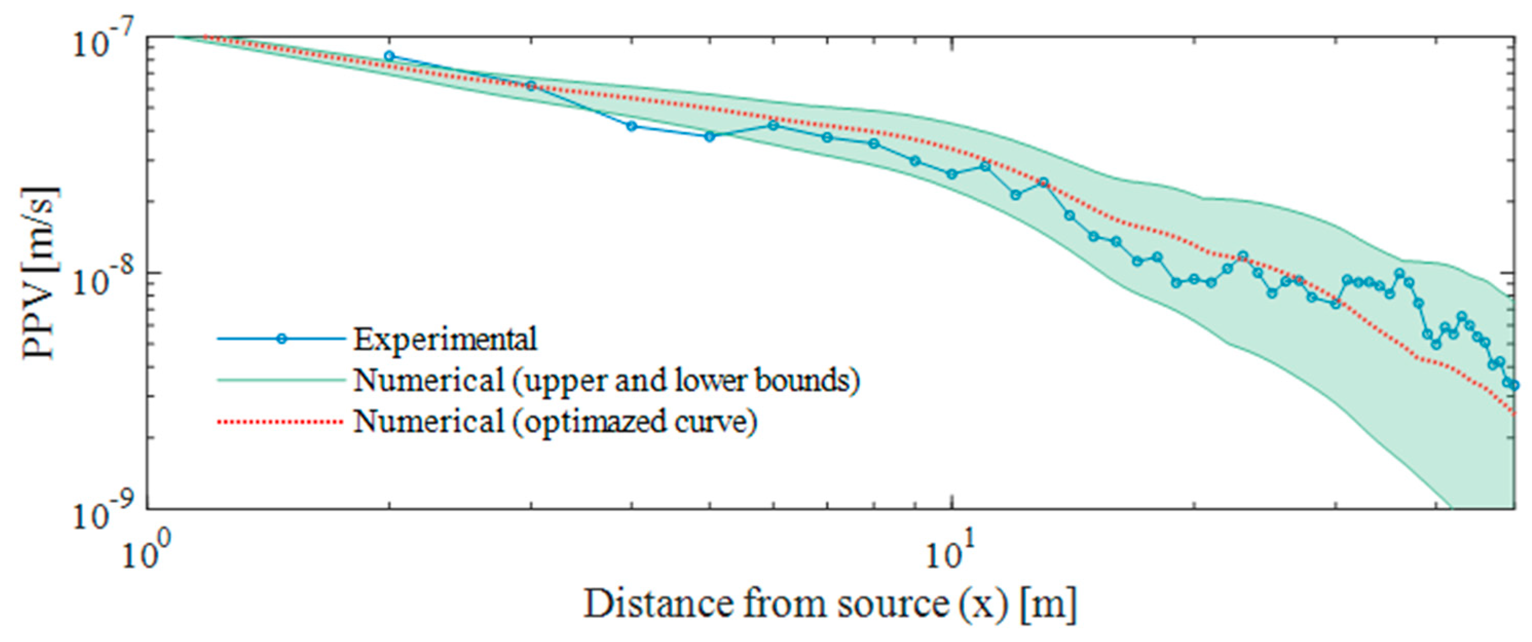
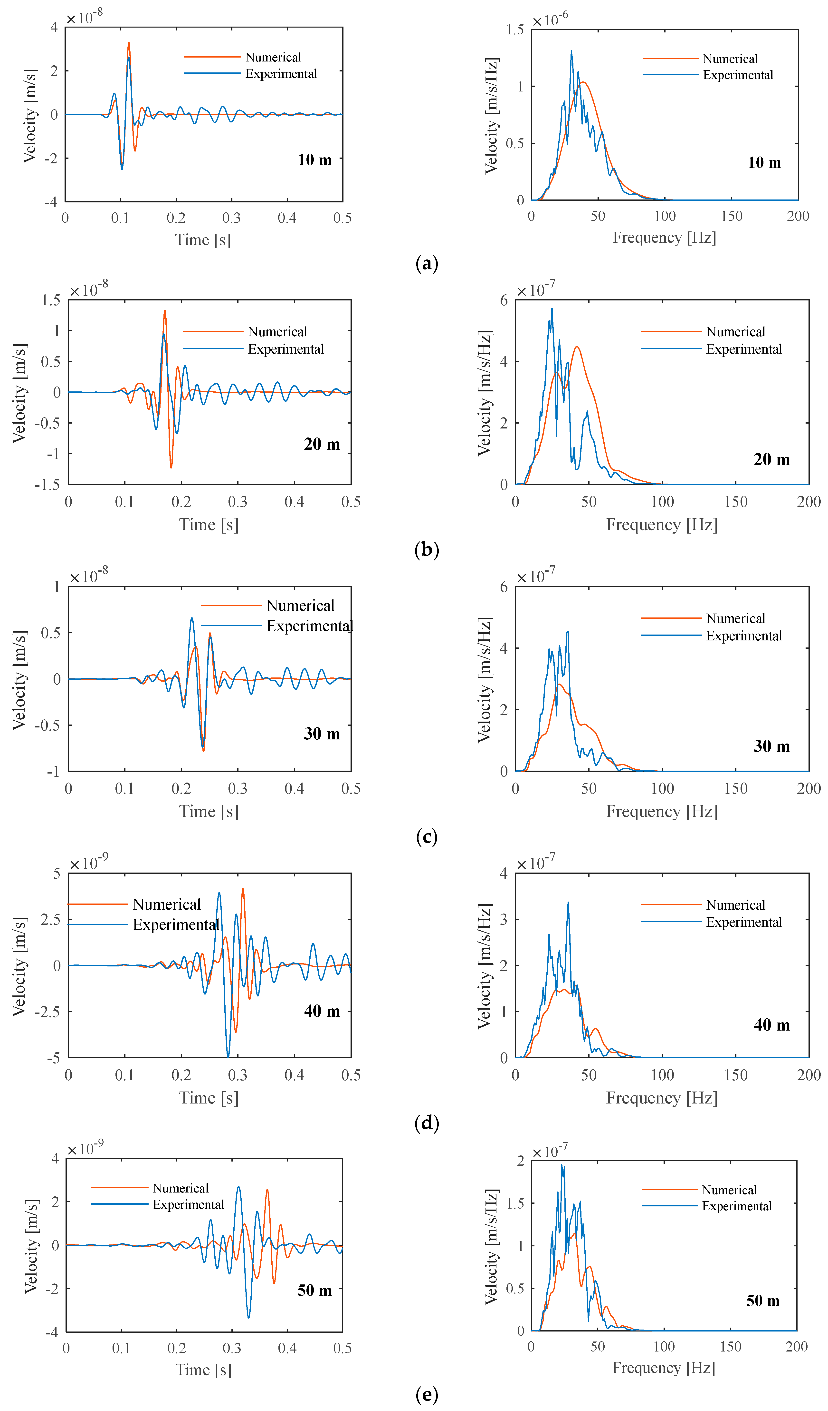
4.3. Comparison between Experimental and Numerical Results

The results obtained in the experimental field and in the numerical model were then compared. Given the uncertainties regarding the material damping of the soil, the numerical simulation comprises two values for this parameter: ξ 1 = 0.01 and ξ 2 = 0.05 . According to the parametric studies performed, the real value of soil damping is included in this range. A damping ratio equal to 5% for the first layer and a value of 2.5% for the remaining layers seems to be a reasonable estimate. The experimental results were compared with the envelope provided by the numerical simulations. Figure 12 presents the comparison in terms of peak particle velocity (PPV) as a function of the distance from the pile center.
The parametric studies emphasize the relevant influence of the material damping of the soil on the dynamic response of the ground, with a relatively constant but wide shaded zone between the limit curves. Despite the uncertainty related to this factor, the line associated with the experimental measurements corresponds to an intermediate case in relation to the predicted numerical envelope. In fact, there is a remarkable agreement between the results across the entire distance. It should be noted that this validation comprises distances up to 50 m from the pile.
Moving on to a more detailed analysis, Figure 13 presents the comparison of the experimental and numerical results in terms of time records and the spectrum of vertical vibration velocities for five different observation points: 10, 20, 30, 40, and 50 m.
In general, there is a satisfactory agreement between the experimental and numerical results. However, as expected, the correspondence between them was greater for the observation points closer to the source. When the observation point was far from the source of impact, some discrepancies occurred. For this occurrence, the volume of soil involved in the response can be identified as an additional factor of uncertainty in the numerical prediction process. In such great distances, effects such as soil inhomogeneity, especially in residual soils, are likely to occur and are not easy to include in a numerical analysis, which justifies the differences between the numerical and experimental results. Notwithstanding, the present numerical model is capable of simulating the main features of the addressed problem.

5. Is Linear Modeling Reasonable for Predicting Vibrations Induced by Pile Driving?

As previously stated, a low dynamic loading was considered, and the analysis presented assumed an elastic and linear soil behavior. However, pile driving operations induce levels of soil strain greater than the compatible elastic limit, as can be seen in Figure 14 [32]. Therefore, the linear approach, assuming low-strain elastic properties of the soil, is usually only acceptable for strains below 10−4 (depending on the type of soil and the confining stress).
Thus, this approach is a simplification of the real behavior of soils, which is highly dependent on the level of induced strain. A typical relationship between secant shear stiffness (G) and damping with shear strain (γ) is presented in Figure 15 [33]. As is well known, the secant shear modulus decreases with induced shear strain, and the opposite occurs with damping.
Aiming at fulfilling the soil dynamic response in the field of representative levels of strain, an equivalent linear analysis can then be integrated into the modeling approach. Therefore, the effects of the non-linear behavior of the soil can be incorporated. This technique addresses an iterative method that compensates for the inelastic behavior by adjusting the parameters of the elastic material for the significant strain levels. The accurate modeling of stiffness degradation with strain is a key feature of the success of this iterative technique.

6. Conclusions

This work presents and explores a properly characterized experimental test site where a low-strain dynamic test was performed. Free-field vibrations due to hammer impact on a driven pile were investigated. These experiments were essential for the validation of a proposed dynamic numerical model for the simulation of the pile–ground system. In this model, formulated under axisymmetric conditions, the finite element method is coupled to perfectly matched layers to avoid spurious reflections in the truncation boundaries of the domain. The experimental results were compared with those predicted by the numerical model. The main conclusions are summarized below:
(i)
Given the uncertainties regarding the material damping of the soil, a parametric study was performed, allowing to discuss the relevant influence of this parameter on the dynamic response of the ground and finding an optimized value that fits the experimental results;
(ii)
The comparison between the experimental and numerical results shows a very satisfactory agreement. This general comment is valid not only in terms of the maximum levels of vibration but also in the frequency range of the response;
(iii)
Given the results obtained, the proposed numerical model can be used in the prediction of ground-borne vibrations for situations where low-strain deformations are expected.
As a final note, the previous studies were conducted assuming a linear behavior of the soil. To predict the vibrations of the ground resulting from impact pile driving, further analysis should comprise the non-linearity effects in the ground simulation. This condition can be easily incorporated into the proposed numerical methodology through an iterative method that compensates for the inelastic behavior by adjusting the elastic properties according to the strain levels observed. The application of the equivalent linear approach in this context will be presented in a subsequent paper by the authors.

Author Contributions

Conceptualization, A.C. and P.A.C.; methodology, A.C., P.A.C., C.P. and A.M.A.; software, A.C., C.P. and A.M.A.; validation, A.C. and A.M.A.; formal analysis, A.C., P.A.C. and C.P.; investigation, A.C., C.P. and A.M.A.; resources, A.C. and P.A.C.; data curation, A.C., P.A.C., C.P. and A.M.A.; writing—original draft preparation, A.C.; writing—review and editing, P.A.C., C.P. and A.M.A.; visualization, A.C. and P.A.C.; supervision, A.C. and P.A.C.; project administration, A.C. and P.A.C.; funding acquisition, P.A.C. All authors have read and agreed to the published version of the manuscript.

Funding

This work was financially supported by Base Funding (UIDB/04708/2020) and Programmatic Funding (UIDP/04708/2020) of the CONSTRUCT—Instituto de I&D em Estruturas e Construções, funded by national funds through the FCT/MCTES (PIDDAC); Project PTDC/ECI-CON/29634/2017 (POCI-01-0145-FEDER-029634), funded by FEDER funds through COMPETE2020—Programa Operacional Competitividade e Internacionalização (POCI) and by national funds (PIDDAC) through FCT/MCTES. Vibration 05 00049 i001

Data Availability Statement

All data used in this work are available from the corresponding author by request.

Conflicts of Interest

The authors declare no conflict of interest.

References

  1. Hindmarsh, J.J.; Smith, W.L. Quantifying construction vibration effects on daily radiotherapy treatments. J. Appl. Clin. Med. Phys. 2018, 19, 733–738. [Google Scholar] [CrossRef] [PubMed] [Green Version]
  2. Rahman, N.A.A.; Musir, A.A.; Dahalan, N.H.; Ghani, A.N.A.; Khalil, M.K.A. Review of vibration effect during piling installation to adjacent structure. AIP Conf. Proc. 2017, 1901, 110009. [Google Scholar]
  3. Athanasopoulos, G.A.; Pelekis, P.C. Ground vibrations from sheetpile driving in urban environment: Measurements, analysis and effects on buildings and occupants. Soil Dyn. Earthq. Eng. 2000, 19, 371–387. [Google Scholar] [CrossRef]
  4. Massarsch, K.R.; Fellenius, B.H. Ground vibrations from pile and sheet pile driving. Part 1 Building Damage. In Proceedings of the DFIEFFC International Conference on Piling and Deep Foundations, Stockholm, Sweden, 21–23 May 2014; pp. 131–138. [Google Scholar]
  5. Cleary, J.C.; Steward, E.J. Analysis of ground vibrations induced by pile driving and a comparison of vibration prediction methods. DFI J.—J. Deep Found. Inst. 2016, 10, 125–134. [Google Scholar] [CrossRef]
  6. Massarsch, K.R.; Fellenius, B.H. Ground vibrations induced by impact pile driving. In Proceedings of the 6th International Conference on Case Histories in Geotechnical Engineering, Arlington, VA, USA, 11–16 August 2008; pp. 1–38. [Google Scholar]
  7. Attewell, P.B.; Farmer, I.W. Attenuation of ground vibrations from pile driving. Ground Eng. 1973, 63, 26–29. [Google Scholar]
  8. Attewell, P.B.; Selby, A.R.; O’Donnell, L. Tables and graphs for the estimation of ground vibration from driven piling operations. Geotech. Geol. Eng. 1992, 10, 61–85. [Google Scholar] [CrossRef]
  9. Massarsch, K.R.; Fellenius, B.H. Engineering assessment of ground vibrations caused by impact pile driving. Geotech. Eng. 2015, 46, 54–63. [Google Scholar]
  10. Whyley, P.J.; Sarsby, R.W. Ground borne vibration from piling. Ground Eng. 1992, 25, 32–37. [Google Scholar]
  11. Grizi, A.; Athanasopoulos-Zekkos, A.; Woods, R.D. Pile Driving Vibration Attenuation Relationships: Overview and Calibration Using Field Measurements. In Geotechnical Earthquake Engineering and Soil Dynamics V: Numerical Modeling and Soil Structure Interaction; American Society of Civil Engineers: Reston, VA, USA, 2018; pp. 435–444. [Google Scholar]
  12. Ramshaw, C.L.; Selby, A.R.; Bettess, P. Ground Waves Generated by Pile Driving, and Structural Interaction. In Proceedings of the International Conferences on Recent Advances in Geotechnical Earthquake Engineering and Soil Dynamics, San Diego, CA, USA, 26–31 March 2001. [Google Scholar]
  13. Khoubani, A.; Ahmadi, M.M. Numerical study of ground vibration due to impact pile driving. Proc. Inst. Civ. Eng. Geotech. Eng. 2014, 167, 28–39. [Google Scholar] [CrossRef]
  14. Homayoun Rooz, A.F.; Hamidi, A. A numerical model for continuous impact pile driving using ALE adaptive mesh method. Soil Dyn. Earthq. Eng. 2019, 118, 134–143. [Google Scholar] [CrossRef]
  15. Sofiste, T.; Godinho, L.; Alves Costa, P.; Soares Júnior, D. An effective time domain numerical model for the prediction of ground-borne vibrations induced by pile driving. In Proceedings of the Inter-Noise 2020, Seoul, Republic of Korea, 23–26 August 2020. [Google Scholar]
  16. Masoumi, H.R.; Degrande, G.; Lombaert, G. Prediction of free field vibrations due to pile driving using a dynamic soil-structure interaction formulation. Soil Dyn. Earthq. Eng. 2007, 27, 126–143. [Google Scholar] [CrossRef]
  17. Masoumi, H.R.; Degrande, G.; Holeyman, A. Pile response and free field vibrations due to low strain dynamic loading. Soil Dyn. Earthq. Eng. 2009, 29, 834–844. [Google Scholar] [CrossRef]
  18. Masoumi, H.R.; François, S.; Degrande, G. A non-linear coupled finite element-boundary element model for the prediction of vibrations due to vibratory and impact pile driving. Int. J. Numer. Anal. Methods Geomech. 2009, 33, 245–274. [Google Scholar] [CrossRef]
  19. Grizi, A.; Athanasopoulos-Zekkos, A.; Woods, R.D. H-Pile Driving Induced Vibrations: Reduced-Scale Laboratory Testing and Numerical Analysis. In Proceedings of the IFCEE 2018 Conference, Orlando, FL, USA, 5–10 March 2018; pp. 165–175. [Google Scholar]
  20. Tsouvalas, A. Underwater Noise Emission Due to Offshore Pile Installation: A Review. Energies 2020, 13, 3037. [Google Scholar] [CrossRef]
  21. Fricke, M.B.; Rolfes, R. Towards a complete physically based forecast model for underwater noise related to impact pile driving. J. Acoust. Soc. Am. 2015, 137, 1564–1575. [Google Scholar] [CrossRef]
  22. Tsouvalas, A.; Metrikine, A.V. Structure-Borne Wave Radiation by Impact and Vibratory Piling in Offshore Installations: From Sound Prediction to Auditory Damage. J. Mar. Sci. Eng. 2016, 4, 44. [Google Scholar] [CrossRef]
  23. Peng, Y.; Tsouvalas, A.; Stampoultzoglou, T.; Metrikine, A. A fast computational model for near- and far-field noise prediction due to offshore pile driving. J. Acoust. Soc. Am. 2021, 149, 1772–1790. [Google Scholar] [CrossRef] [PubMed]
  24. Berenger, J. A perfectly matched layer for absorption of electromagnetic waves. J. Comput. Phys. 1994, 114, 185–200. [Google Scholar] [CrossRef]
  25. Johnson, S.G. Notes on Perfectly Matched Layers (PMLs). arXiv 2021, arXiv:2108.05348. [Google Scholar]
  26. Lopes, P.; Costa, P.A.; Ferraz, M.; Calçada, R.; Cardoso, A.S. Numerical modeling of vibrations induced by railway traffic in tunnels: From the source to the nearby buildings. Soil Dyn. Earthq. Eng. 2014, 61–62, 269–285. [Google Scholar] [CrossRef]
  27. Lopes, P.; Alves Costa, P.; Calçada, R.; Silva Cardoso, A. Numerical Modeling of Vibrations Induced in Tunnels: A 2.5D FEM-PML Approach. In Traffic Induced Environmental Vibrations and Controls: Theory and Application; Xia, H., Calçada, R., Eds.; Nova: Hauppauge, NY, USA, 2013; pp. 133–166. [Google Scholar]
  28. Masoumi, H.; Degrande, G. Numerical modeling of free field vibrations due to pile driving using a dynamic soil-structure interaction formulation. J. Comput. Appl. Math. 2008, 215, 503–511. [Google Scholar] [CrossRef] [Green Version]
  29. Deeks, A.; Randolph, M. Analytical Modeling of Hammer Impact for Pile Driving. Int. J. Numer. Anal. Methods Geomech. 1993, 17, 279–302. [Google Scholar] [CrossRef]
  30. Degrande, G.; Badsar, S.A.; Lombaert, G.; Schevenels, M.; Teughels, A. Application of the coupled local minimizers method to the optimization problem in the spectral analysis of surface waves method. J. Geotech. Geoenviron. Eng. 2008, 134, 1541–1553. [Google Scholar] [CrossRef]
  31. Ricker, N. The form and laws of propagation of seismic wavelets. Geophysics 1953, 18, 10–40. [Google Scholar] [CrossRef]
  32. Zekkos, A.A.; Woods, R.D.; Grizi, A. Effect of Pile-Driving Induced Vibrations on Nearby Structures and Other Assets. Michigan Department of Transportation; Report: ORBP Number OR10-046; University of Michigan: Ann Arbor, MI, USA, 2013. [Google Scholar]
  33. Szilvágyi, Z.; Ray, R. Measuring and Modeling the Dynamic Behavior of Danube Sands. In Proceedings of the 18th International Conference on Soil Mechanics and Geotechnical Engineering: Challenging and Innovations in Geotechnics, Paris, France, 2–6 September 2013. [Google Scholar]
Figure 1. Representative scheme of the numerical modeling approach.
Vibration 05 00049 g001
Figure 2. Pile–ground system model using an axisymmetric FEM-PML numerical approach.
Vibration 05 00049 g002
Figure 4. Free vibration (blue line) and truncated force (red line) applied at the anvil surface.
Vibration 05 00049 g004
Figure 5. Experimental test site: (a) general view; (b) geological–geotechnical profile; (c) foundation plan and borehole’s location (S1–S7).
Vibration 05 00049 g005aVibration 05 00049 g005b
Figure 6. Dynamic characterization of the soil: (a) setup for the experimental activities; (b) experimental P-SV dispersion relationship.
Vibration 05 00049 g006
Figure 7. Dynamic properties of the soil along the depth: (a) S-wave velocity profile; (b) P-wave velocity profile.
Vibration 05 00049 g007
Figure 8. Example of the impact hammer force: (a) time history; (b) frequency content.
Vibration 05 00049 g008
Figure 9. Experimental setup used for low-strain test.
Vibration 05 00049 g009
Figure 10. FE–PML mesh adapted to model the pile–ground system.
Vibration 05 00049 g010
Figure 11. Ricker pulse: (a) time history; (b) frequency content.
Vibration 05 00049 g011
Figure 12. Peak particle velocity versus distance from the pile due to Ricker pulse: experimental (blue line) vs numerical results (red line— ξ = 0.05   f i r s t   l a y e r ;   0.025   r e m a i n i n g   l a y e r s ; upper bound— ξ 1 = 0.01 ; lower bound— ξ 2 = 0.05 ).
Vibration 05 00049 g012
Figure 13. Experimental velocities of vertical vibration measured at different distances from the pile compared to the numerical prediction for a material damping ratio equal to 0.025: (a) 10 m; (b) 20 m; (c) 30 m; (d) 40 m; (e) 50 m (left: time history; right: frequency content).
Vibration 05 00049 g013
Figure 14. Hypothetical soil behavior zones near a driven pile.
Vibration 05 00049 g014
Figure 15. Stiffness degradation and damping increase with shear strain for sand and clay.
Vibration 05 00049 g015
Table 1. Elastodynamic properties of the pile–ground system (E—Young’s modulus; ν—Poisson’s ratio; ρ—mass density; ξ—hysteretic damping factor).
Elementh (m)E (MPa)ν (-)ρ (kg/m3)ξ (%)
Soil21540.2519005
62510.252.5
56200.49
inf22000.49
PileL = 12 m30,0000.2025001
Publisher’s Note: MDPI stays neutral with regard to jurisdictional claims in published maps and institutional affiliations.

