Bearing Fault Diagnosis Based on Multi-Scale CNN and Bidirectional GRU

Abstract

Finding a reliable approach to detect bearing faults is crucial, as the most common rotating machine defects occur in its bearings. A convolutional neural network can automatically extract the local features of the mechanical vibration signal and classify the patterns. Nevertheless, these types of networks suffer from the extraction of the global feature of the input signal as they utilize only one scale on their input. This paper presents a method to overcome the above weakness by employing a combination of three parallel convolutional neural networks with different filter lengths. In addition, a bidirectional gated recurrent unit is utilized to extract global features. The CWRU-bearing dataset is used to prove the performance of the proposed method. The results show the high accuracy of the proposed method even in the presence of noise.

1. Introduction

Rotary machines have an undeniable role in industry. They are widely used in a variety of industrial applications. Under adverse conditions such as improper lubrication, overload, high temperature, and high humidity, these machines will eventually be damaged. Bearing failure is one of the most common failures in rotary machines, so the proper performance of bearings has a great impact on the efficiency of these machines. It is reported that more than 45% of all failures are due to defective bearings [1,2]. It is clear that early fault detection is crucial to ensure the safety and proper operation of rotating machines, so that severe faults, failures, and higher repair costs can be prevented by identifying faults in the early stages.

Fault detection methods are generally divided into three categories: (1) model-based methods or “white box”, (2) machine learning-based methods or “black box”, and (3) a combination of the above two methods or “gray box”.

In model based fault diagnosis, existence of a model for the system under study is crucial. Based on this model, residuals are generated for identifying faults. Unfortunately, this approach fails when there is uncertainty in the model or measurement data are noisy. Another promising approach is machine learning based or data-driven based fault diagnosis. This approach is very attractive where there is no model or uncertainty of the model is high. In this approach, only data are used for fault diagnosis. The main drawback of this scheme is that it is heavily depends on having a high-quality extensive training database. Currently, a hybrid approach is proposed to reduce the drawbacks of these two approaches and enhance the accuracy of the fault diagnosis process. In this new scheme, residuals generation is done by a model-based method and residual selection is applied by a machine learning-based approach [3]. One example of such an approach can be found in [4].

Currently, machine learning, including classical machine learning methods and deep learning methods, has provided the basis for intelligent fault diagnosis. Classical (shallow) machine learning methods only work on handicraft features (features that are manually and artificially extracted from the signal). As a consequence, these methods do not take advantage of all the features that are potentially present in the input data.

In [5,6], spectral analysis of a motor current is used to detect bearing faults in electric motors. Faults in the bearing result in torque fluctuations, which results in a change in the frequency spectrum of the stator current. The amplitude of the added frequencies to the stator current substantially depends on the bearing type and the load conditions. Ref. [7] benefits from the combination of accelerometer and load cell data and the utilization of k-nearest neighbors (KNN) to detect bearing faults. Based on the results, the data obtained from the load cell are useful for detecting the fault, and the accelerometer is useful for identifying the location of the fault. Reference [8] uses the iterative Boolean combination (IBC) technique, a strategy based on the combination of different support vector machines (SVMs), which aims to reduce the effect of noise on the fault detection system. According to the experiments, even in the presence of noise, this system can detect faults in a bearing. In [9], higher-order spectral (HOS) and SVM were used to classify four types of bearing fault in different working conditions. Results show that it is a powerful method for detecting faults in rotary machines, but this method also requires manual feature extraction.

In deep learning-based models, features of the input data are extracted automatically, without human intervention. In [10], an engine condition monitoring system was proposed using a one-dimensional convolutional neural network (1DCNN) that connects the two main parts of a fault detection system: the feature extraction and the classification parts. This model has good generalization and eliminates the need to manually extract the features. Generated images of vibration data in the time–frequency domain were used in [11] to identify bearing faults. To this end, those images were analyzed by deep convolutional networks. It turned out that this architecture is resistant to noise. Ref. [12] forms a matrix by combining multi-sensor data and considering them as the input to the convolutional network. By comparing the results of this method with the traditional ones, it was concluded that CNN has a better and more reliable diagnostic performance. In [13], a deep recurrent neural network is ameliorated by an augmentation of recurrent hidden layers. In this method, the frequency spectrum of the vibration signal is used as input. The results confirm that this method has a better performance compared to other intelligent methods. Ref. [14] uses the convolutional network and long short-term memory (LSTM) with the attention mechanism. In this model, the raw vibration signal was used, accompanying its frequency spectrum as the model input. Moreover, the attention mechanism was used to pay more attention to the distinguishing features. The proposed fault identification method in reference [2] is called S-transform CNN (ST-CNN), which is presented using the ST layer and convolutional neural network. The input vibration signal in the ST layer is converted to a two-dimensional time-frequency matrix. Then, it enters the convolutional network. Finally, it classifies by the maximum softmax layer. Compared to other methods, such as short-time Fourier transform (STFT) + CNN, SVM, and KNN, the results show that the diagnostic performance of this method can be more promising and more reliable for diagnosing bearing faults. Reference [15] proposed a deep learning method based on a combination of stacked residual dilated convolutional neural network (SRDCNN) and LSTM. The structure of LSTM can effectively eliminate the effects of noise. In [16], a multilayer bidirectional gated recurrent unit with an attention mechanism (Att-MBiGRU) network was used. In comparison with different models, the results show that the attention mechanism helps the network to perform better in noisy conditions. Reference [17] proposes a bidirectional recurrent neural network (RNN-WDCNN) consisting of a 5-layer convolutional neural network plus a pathway combining elements of recurrent neural networks and convolutional neural networks. The recurrent neural network used in this model is efficient for learning long-term dependencies in time-series data and eliminating high-frequency noise in the input signal. According to the authors, the inclusion of the attention mechanism in the return path of the model did not have a significant effect on noise effect reduction. In [18], the raw data collected by the accelerometer sensor were considered as input to the CNN + LSTM algorithm and fault detection, so it can be said that, like most deep learning methods, it did not use selective data features and had a relatively good performance. Time–frequency signature matrix (T–FSM) feature sensitive to few-shot vibration signal and multi-label convolutional neural network with meta-learning (MLCML) was proposed in [19]. Ref. [20] proposed a pseudo-categorized maximum mean discrepancy (PCMMD) and used it to drive the multi-input multi-output convolutional network (MIMOCN) to narrow the cross-domain distribution discrepancy of the deep feature space.

Single-scale convolutional neural network-based models use only a certain scale of the signal in the first layer, whereas the mechanical vibration signal has different frequencies and different potential features at different time scales. Unfortunately, single-scale convolution may lead to the loss of this potential information. Therefore, multi-scale convolutional networks were proposed. In [21], a shallow convolutional neural network, multi scales CNN combined with a multiple attention model called MA-MSCNN, was proposed. According to the results, 99.86% accuracy was achieved with this method. In [22], in order to automatically extract the frequency features, two convolutional neural networks with different kernel sizes were used, and LSTM was used to identify the type of fault. In [23], a multi-scale deep convolutional neural networks (MS-DCNN) model was presented. Based on the results, the MS-DCNN model could achieve higher accuracy compared to 1D-CNN and 2D-CNN. In this study, an improved multi-scale convolutional neural network integrated with a feature attention mechanism has been developed to overcome the weaknesses of CNN-based models under noisy environments.

The proposed method in this paper tries to overcome the aforementioned weaknesses. The contributions of this paper can be summarized as follows:

• The proposed method employs a multi-scale structure and bidirectional recurrent network to extract and combine spatial and temporal features available at different frequencies of the input vibration signal.
• Despite extensive filters and pooling in the convolutional network, the model achieves high generalizability.
• In this method, the adaptive gradient optimization algorithm is used, so the performance of the model is independent of the selection of the optimal learning rate, and there is no need to find the best learning rate value.
• With batch normalization + exponential linear unit (BN + ELU), the convergence speed of the model will be very fast and needs fewer iterations to converge.
• In comparison to other schemes, the proposed method has an excellent performance in classifying the types of faults and shows robustness to noise.

The structure of the paper is as follows: Section 2 is devoted to the basic concepts. Section 3 introduces the proposed model architecture. In Section 4, the performance of the proposed model is evaluated through the Case Western Reserve University (CWRU) bearning dataset. Finally, the paper is concluded in Section 5.

2. Definitions

In this section, some essential definitions that are employed in the proposed method are introduced.

2.1. Convolutional Neural Network (CNN)

Convolutional neural networks were developed in 1990 with inspiration from the visual cortex [24]. A convolutional neural network is a feedforward neural network capable of processing data with grid-like topology (e.g., imagery data).

In fully connected neural networks (FCs), each neuron in each layer connects to all neurons in the next layer, and each connection between neurons (weights) will be a parameter in the network, so these networks will have too many training parameters for high-dimensional input data.

In contrast to fully connected networks, convolutional networks create local connections between neurons, i.e., each neuron connects only to the nearby neuron in the next layer. Moreover, the connections between the input and the neurons use a set of common weights called the convolution kernel. These two properties in convolutional networks have made it possible to process high-dimensional data. Supremely, local connectivity and weight sharing lead to local network input feature extraction.

A convolutional layer has at least one filter that performs convolutional operations. The result of these calculations is called the feature map. Hence, each “feature map” includes features extracted by different filters. Each filter in the convolutional network extracts unique features out of the training data. The number and size of these filters are defined in the network hyperparameters.

Here, a one-dimensional convolutional neural network (1DCNN) is introduced, as the input data of this study are mechanical vibration signals. If the input time series data are considered as X, then:

$$X=\left[x_1,x_2,\dots ,x_N\right]$$

(1)

where N is the length of the data entry window. In this case, the time series sequence will be as in Equation (2).

$${\mathrm{X}}_{i:i+F_L-1}=\left[x_i,x_{i+1},\dots ,x_{i+F_L-1}\right]$$

(2)

The convolution could be assumed as a multiplication between the filter kernel W and the input data ${\mathrm{X}}_{i:i+F_L-1}$, where $F_L$ is the length of the convolution filter. The feature map obtained from the input data by convolution is in vector form and is called $z_i$. Feature vectors eventually pass the nonlinear activation function, as introduced in Equation (3):

$$z_i=\phi (W^T{\mathrm{X}}_{i:i+F_L-1}+b)$$

(3)

where b and $\phi$ are bias and nonlinear activation function, respectively. Finally, the feature map is obtained by putting these feature vectors together.

$$z_j=\left[z_j^1,z_j^2,\dots ,z_j^{N-F_L+1}\right]$$

(4)

Then, maxpooling [14] is applied to the feature map to reduce feature dimensions and prevent overfitting; $p_j$ is the output of the maxpooling layer applied to the feature map extracted by the jth filter.

$$p_j=\left[p_j^1,p_j^2,\dots ,p_j^s\right]$$

(5)

where s is the number of remaining features after maxpooling. By expanding each $p_j$, the maxpooling relation is as in Equation (6):

$$p_j^k=max\left(z_j^{(k-1)g+1},z_j^{(k-1)g+2},\dots ,z_j^{kg}\right)$$

(6)

where $k=1,2,\cdots ,K_{max}$, where $K_{max}\times g=$ length of feature vector, g is the length of the pooling, and $p_j$ is the pooling layer output applied to the jth feature map.

2.2. Gated Recurrent Unit

A recurrent neural network (RNN) is suitable for processing time series and sequential data. Recurrent neural networks have an internal memory and can store previous information in their cells. To train RNNs at each time step, the error gradient is obtained using the backpropagation through time (BPTT) algorithm, and the network parameters are adjusted accordingly.

If the length of the input sequence or the network depth in a typical RNN increases, then the gradient vanishing/exploding problem will occur and stops the training process. Thus, RNNs are not capable of learning long data dependencies. Therefore, long short-term memory (LSTM) was introduced to overcome this problem [25].

LSTM solved simple RNN problems because it had a forget gate. The gated recurrent unit (GRU), which is based on LSTM, was proposed in [26]. The only difference is that it has fewer gates and uses fewer training parameters, so it has a faster training process. The training speed is 29.29% faster than with LSTM, and the ratio of accuracy to computational cost is 23.45% more than LSTM [27], and it has performed better than LSTM to maintain long-term dependencies [28].

An important distinguishing feature between typical RNN and GRU is the ability to control the hidden information that solves gradient issues. This is possible in GRU through two gates. For instance, if the input is very important in a time step, the GRU will learn not to forget its information and keep it in a hidden status. Likewise, if the input is irrelevant and insignificant, GRU learns to ignore it. 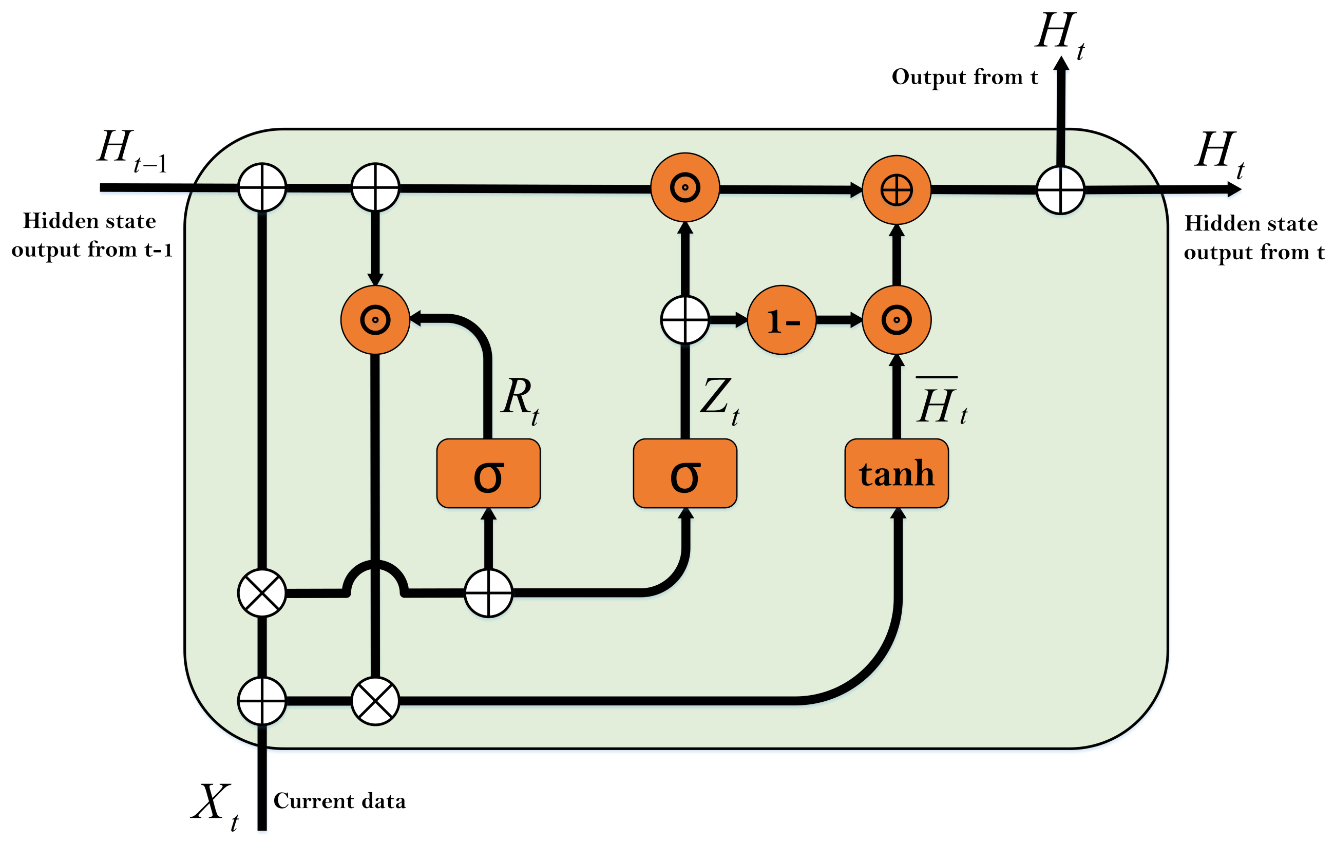Figure 1 depicts the block diagram of one cell in the GRU network.

The reset gate determines how much of the previous hidden state is maintained, and the update gate controls how much of the previous time step of hidden mode is selected as the next time step of the hidden state and how much of the current time step knowledge is added to the hidden state. These gates make their decisions based on two criteria: the current input and the hidden state of the previous time step. These two criteria are fed to a fully connected neural network with a sigmoid activation function. The sigmoid activation function maps the input values to the range between 0 and 1 and creates the concept of a gate.

The relationships used in these gates are as in Equation (7):

$$\begin{array}{cc}\hfill R_t& =\sigma \left(W_r{X}_t+U_r{H}_{t-1}\right)\hfill \\ \hfill Z_t& =\sigma \left(W_z{X}_t+U_z{H}_{t-1}\right)\hfill \\ \hfill {\overline{H}}_t& =tanh\left(\left(W_H{X}_t\right)+U_H(R_t\odot H_{t-1})\right)\hfill \\ \hfill H_t& =\left(Z_t\odot H_{t-1}\right)+\left(\left(1-Z_t\right)\odot {\overline{H}}_t\right)\hfill \end{array}$$

(7)

where $r_t$ is the reset gate, $z_t$ is the update gate, $W_r$ and $W_z$ are the weights connected to the input vector, $U_r$ and $U_z$ are the weights connected to the previously hidden status, and ⊗, ⊕, and ⊙ are concatenate, copy, and product, respectively.

Next, the candidate’s hidden state is obtained to be present in the final time step, based on the information generated in the current time step and the previous hidden state, as in Equation (8):

$$g_t=tanh\left(W_g{X}_t\right)\oplus U_g\left(R_t\otimes H_{t-1}\right)$$

(8)

where $W_g$ is the weights attached to the input vector, g is a candidate for the hidden state, and the tanh activation function is used to keep the values in the hidden state between $-1$ and 1. The generated g is only one candidate and depends on the performance of the update gate. Finally, it is the update gate $z_t$ that determines how much of the candidate’s hidden state is used and how much of the previous hidden state remains in the current hidden state. The final hidden state is updated in time step t according to Equation (9):

$$H_t=\left(\left(1-Z_t\right)\otimes H_{t-1}\right)\oplus \left(Z_t\otimes g_t\right)$$

(9)

If $Z_t$ is close to zero, the hidden state will be kept and the candidate’s hidden state will be ignored. Conversely, if $Z_t$ is close to one, the newly generated hidden state will be approximately the same as the candidate’s hidden state. Therefore, the factors that overcome the gradient issues and keep long-term dependencies in the recurrent neural networks are the gates.

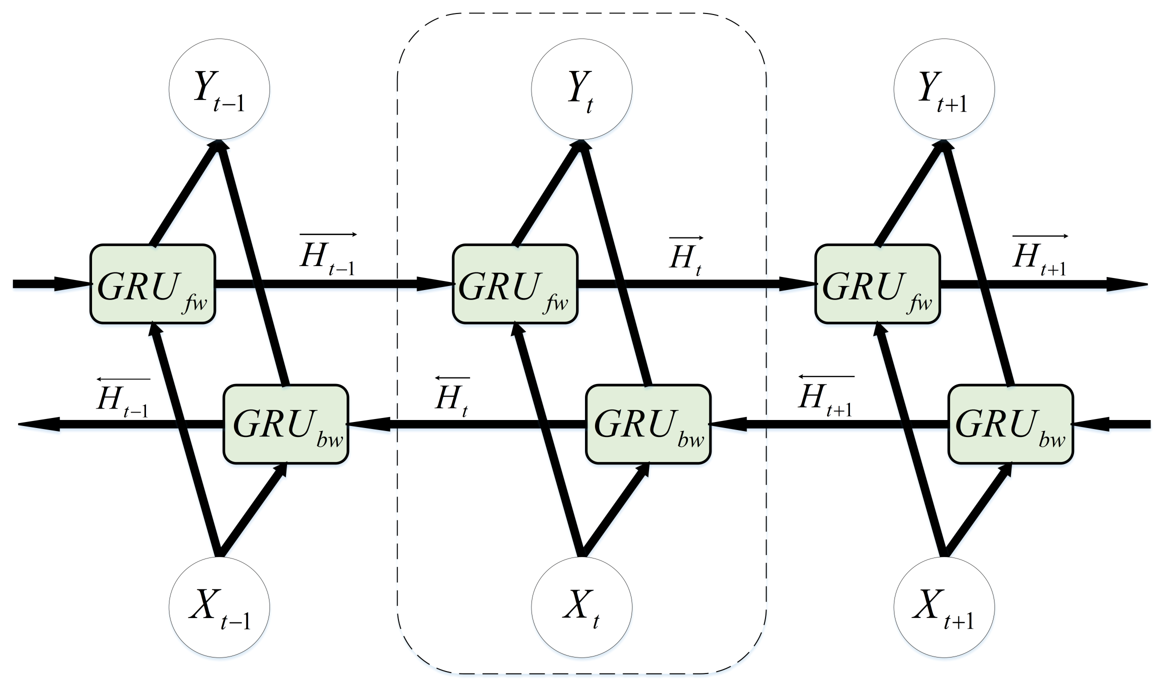
2.3. Bidirectional Gated Recurrent Unit

A typical recurrent neural network learns sequential information in one direction, i.e., the dependence of the time step t to the previous temporal steps, but potentially available information will be lost, i.e., the dependence of the previous moments to the subsequent moments. Hence, [30] suggests the bidirectional gated recurrent unit (BiGRU). In a BiGRU, a GRU layer is added to process the backward data, causing the $y_t$ output at time t to be based on the information of the previous time steps ($H_{t-1}$) as well as the information of the next time steps ($H_{t+1}$). Figure 2 shows a BiGRU.

The forward hidden GRU layer (${\overrightarrow{H}}_t$) and the backward hidden GRU layer (${\overleftarrow{H}}_t$) is defined as in Equation (10).

$$\begin{array}{c}\hfill \begin{array}{cc}\hfill \overrightarrow{H_t}& =GR{U}_{fw}\left(\overrightarrow{H_{t-1}},X_t\right)\hfill \\ \hfill \overleftarrow{H_t}& =GR{U}_{bw}\left(\overleftarrow{H_{t+1}},X_t\right)\hfill \\ \hfill Y_t& =\left[\overrightarrow{H_t};\overleftarrow{H_t}\right]\hfill \end{array}\end{array}$$

(10)

2.4. Batch Normalization (BN)

Training deep neural networks and convergence of the parameters is a difficult task due to the large number of layers. Data preprocessing can have a huge impact on deep network training. S. loffe [31] proposed a preprocessing method to overcome the internal covariate shift during deep neural network training called batch normalization (BN). When the statistical distribution of input to a learning system changes, it is called the internal covariate change phenomenon of the learning system [32]. During the training process, the layers try to adapt to the new distribution, so this phenomenon is problematic and slows down the training process, limiting the choice of a high learning rate. To deal with such problems, BN normalizes the statistical distribution of the batch at the input of each layer. In each iteration, the mean and standard deviation of training data of each batch is calculated and its data are normalized by subtracting the mean and dividing by the standard deviation. Therefore, the normalization of each input in BN is based on the statistical properties of its respective batch. if a batch with size n is considered as a sample, the mean and standard deviation of the batch in layer l is calculated as in Equation (11):

$$\begin{array}{cc}\hfill {\mu }_l& =\frac{1}{n}\sum _{i=1}^n{Z}_{l,i}\hfill \\ \hfill {\sigma }_l^2& =\frac{1}{n}\sum _{i=1}^n{\left(z_{l,i}-{\mu }_l\right)}^2\hfill \end{array}$$

(11)

The normalized value of each sample in layer l is calculated with Equation (12):

$${\widehat{z}}_{l,i}=\frac{z_{l,i}-{\mu }_l}{\sqrt{{\sigma }_l^2+\epsilon }}$$

(12)

where $ϵ$ is a small constant and is added to the variance just to avoid possible division by zero. Finally, BN is applied to the ith samples in layer l as in Equation (13):

$${\tilde{z}}_{l,i}={\gamma }_{l,i}\ast {\widehat{z}}_{l,i}+{\beta }_{l,i}$$

(13)

where a coefficient ($\gamma$) and a deviation ($\beta$) are considered for that BN. These two parameters allow the learning algorithm to learn how to optimally use the BN. For example, if normalizing some features makes network performance worse, the learning algorithm will neutralize the normalization by these two parameters. Therefore, by learning the optimal $\gamma$ and $\beta$ parameters, the learning process will determine the appropriate BN. By normalizing the distribution of input data and preventing the internal covariate shift in a network, BN will provide positive effects. BN allows using high learning rates without any possible gradient divergence [31].

In fully connected layers, BN is usually applied before the activation function and normalizes the function input with Equation (14):

$$h=\varphi \left(BN\left(wx+b\right)\right)$$

(14)

where $\varphi$ is an activation function.The BN applied to each input sample will be determined by the statistical properties of the corresponding batch. BN differs from convolutional networks because the different elements of the feature map must be normalized equally to maintain the property of temporal features in the convolution. For example, if the batch has m instances and each feature map has dimensions $w\times h$, BN will be performed on all $m\times w\times h$ elements based on the mean and standard deviation of batch input samples.

2.5. Exponential Linear Unit Activation Function

Clevert et al. [33] introduced an improved version of the rectified linear unit (ReLU) activation function and its variants, i.e., parametric rectified linear unit (PReLU) and LeakyReLU, also called the exponential linear unit (ELU). This function is defined in Equation (15).

$$\mathrm{elu}\left(x\right)=\left\{\begin{array}{c}\hfill \alpha (exp(x)-1)\mathrm{if}x\le 0\hfill \\ \hfill x\mathrm{if}x>0\hfill \end{array}\right.$$

(15)

where $\alpha$ is a hyperparameter and specifies the value to which the ELU converges for negative inputs. The ELU gradient is based on Equation (16).

$$\frac{d}{dx}\mathrm{elu}\left(x\right)=\left\{\begin{array}{c}\hfill \mathrm{elu}\left(x\right)+\alpha \mathrm{if}x\le 0\hfill \\ \hfill 1\mathrm{if}x>0\hfill \end{array}\right.$$

(16)

Like the ReLU, the ELU solves the gradient vanishing issue by having a single gradient for all positive inputs. In conjunction with accelerating the deep network learning compared to other functions of the ReLU family, the ELU provides better generalizability in the model [33].

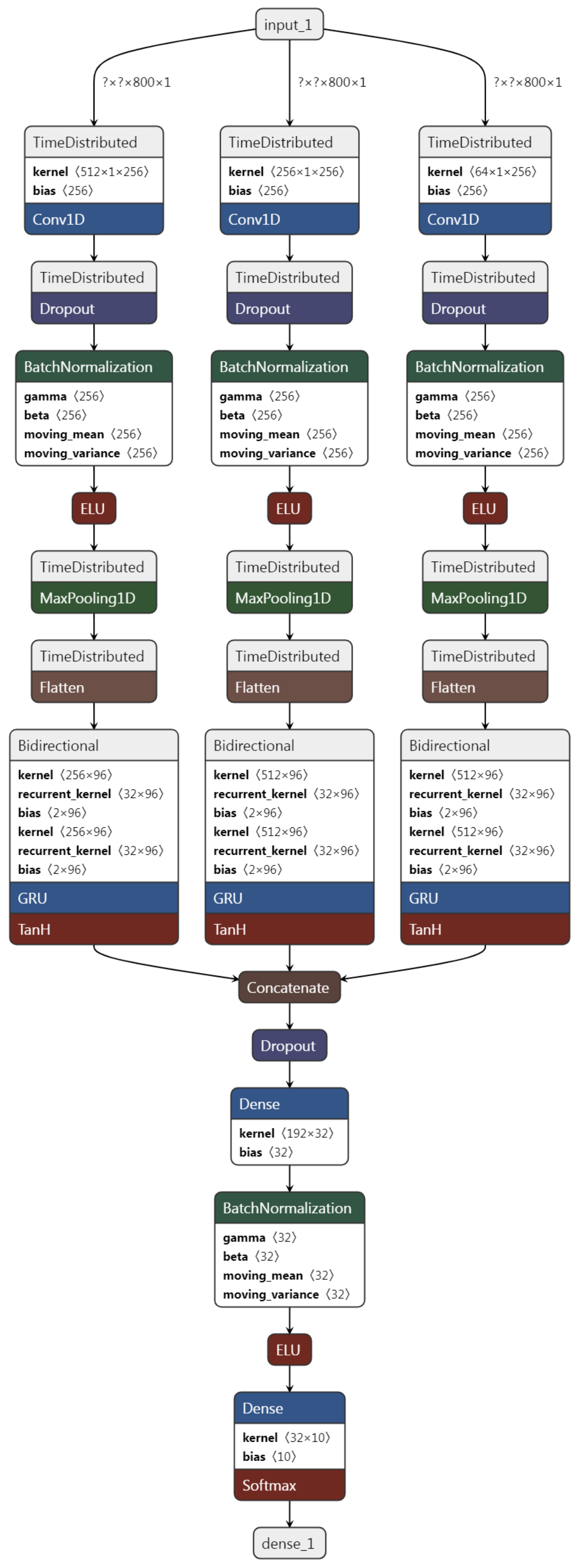
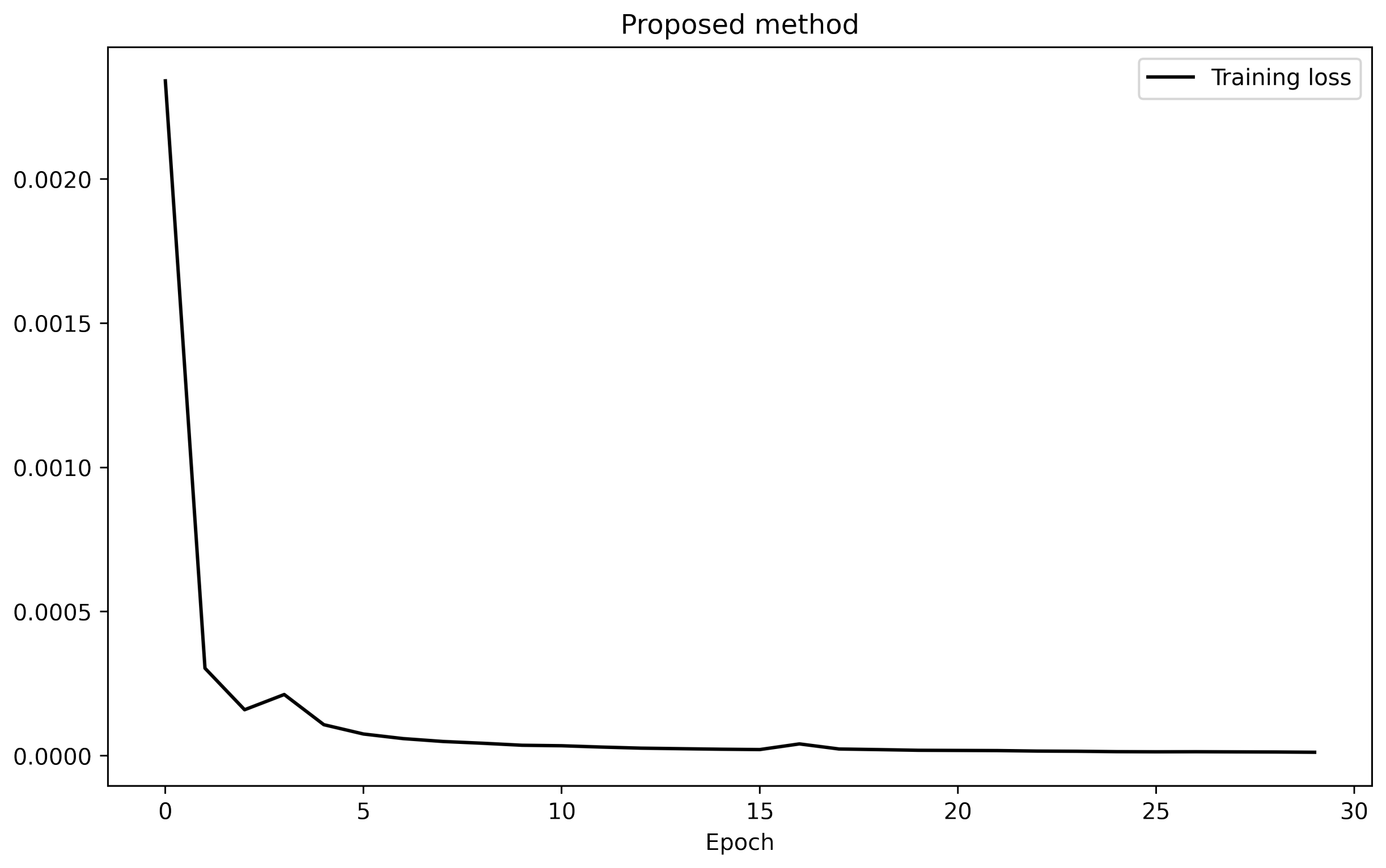
3. Proposed Model

The proposed structure consists of several different layers to establish a relationship between the raw bearing vibration signal and the output label. In the first layer, the convolutional network is used to extract the local features of the vibration signal. Each convolutional neural network contains a number of filters that extract their patterns by moving on the signal. In each layer, the size of these filters is fixed, and the convolution filter solely observes a certain range of signals in each slip.

Therefore, if multiple scales and frequencies of the vibration signal could be monitored, then more complete information about the signal could be achieved. In this regard, three parallel convolutions are used in the proposed model, each of which has a specific filter size, and each convolution has to extract features related to its scale.

All three convolutions have 256 one-dimensional filters, but the length of the filter is different. The length of the filters for the first convolution is 512, which is relatively large for an input vibration signal, and includes a signal with a length of 800, so they will be able to extract low-frequency features. The length of the second convolution filter is 256, which extracts the intermediate frequency features. In addition, in order not to lose the high-frequency features, a convolution layer with filters of length 64 is applied. Each convolution layer output will be feature maps that are the results of a specific scale of the input signal.

Dropout is applied after each layer. Dropout is a simple mechanism that turns off a number of neurons during the training process, and the weight of the connections of those neurons is not updated. The dropout rate is selected to be 0.05. This makes the network less sensitive to small changes in the input data, thus increasing the network’s generalizability and preventing overfitting.

Maxpooling is used to summarize the feature map and reduce the feature dimensions. The maxpooling output of a feature map contains the most prominent input features. The maxpooling window intended for the proposed model is equal to 256, which makes the resulting feature map small.

In each channel, after the convolutional network, a bidirectional GRU is used to extract global information and learn the sequential information of the feature map obtained by the convolution layer. A bidirectional GRU layer is used at the end of each channel to find the temporal dependencies between the spatial features obtained from the convolutional network. The bidirectional GRU extracts sequential information in both directions (dependence of before–after and post-forward moments) and learns the sequential pattern in the local features extracted by convolution. In the next step, all local and global features obtained from different signal scales are merged. In the final step, a fully connected (FC) layer with 32 neurons categorizes the extracted features. In this layer, like the convolutional network, batch normalization (BN) and ELU activation functions are applied.

The softmax function is used to find out the probability of which input data belong to a specific category. This output function converts the output of a network to a probability distribution with Equation (17):

$$\begin{array}{c}\hfill \sigma {\left(\mathbf{z}\right)}_i=\frac{e^{z_i}}{{\sum }_{j=1}^K{e}^{z_j}}\mathrm{for}i=1,\dots ,K\\ \hfill \mathrm{and}\mathbf{z}=(z_1,\dots ,z_K)\in {\mathcal{R}}^K\end{array}$$

(17)

In the above relation, K is the number of output neurons, z is the input vector of the function, and i is the index of the input vector. The neuron with the highest value of the function represents the class to which the provided input belongs. To calculate the network output error, the mean squared logarithmic error (MSLE) loss function is used, which is a type of mean squared error (MSE) loss function, and it has the advantage that small and big errors behave in a logarithmic manner. This function is defined in Equation (18):

$$MSLE=\frac{1}{n}\sum _{i=1}^n(log(y_i+1)-log({\widehat{y}}_i+1){)}^2$$

(18)

where $\widehat{y}$ is the network output, y is the true output, and n is the number of data. To update the weights, an adaptive gradient algorithm (Adagrad) is used. This algorithm is defined in Equation (19).

It should be noted that adaptative gradient (Adagrad) is a feature-specific learning rate optimizer. The adaptation of the learning rate is related to the frequency of update of a given feature. It assigns a higher learning rate to the infrequent features and vice versa.

$$\begin{array}{cc}\hfill {\theta }_{t+1,i}& ={\theta }_{t,i}-\frac{\eta }{\sqrt{G_{t,ii}+\epsilon }}·g_{t,i}\hfill \\ \hfill g_{t,i}& ={\nabla }_{{\theta }_t}J\left({\theta }_{t,i}\right)\hfill \end{array}$$

(19)

where $G_t\in {\mathcal{R}}^{d\times d}$ is a diagonal matrix whose elements are the sum of gradients with respect to ${\theta }_i$ to time t, and $ϵ$ is a fixed number to avoid dividing by a possible zero. The architecture of the proposed model is shown in Figure 3. All hyperparameters of the proposed method are presented in

Table 1. Proposed model hyperparameters.

	Layer Name	Parameter	Value
Architecture	Input	-	800 × 1
	MS_CNN1D	Kernels 1, 2, 3	256
		Kernels size 1	512
		Kernels size 2	256
		Kernels size 3	64
	Dropout	Rate	0.05
	BN	Momentum	0.99
	ELU	Alpha	1
	MaxPooling1D	Pool size	256
	BiGRU	Units	32, 32
	Dropout	Rate	0.05
	Dense	Units	32
	BN	Momentum	0.99
	ELU	Alpha	1
	Dense	Units	10
Training		Epochs	30
		Batch size	128
		Learning rate	0.5
		Loss function	MSLE
		Optimizer	AdaGrad

.

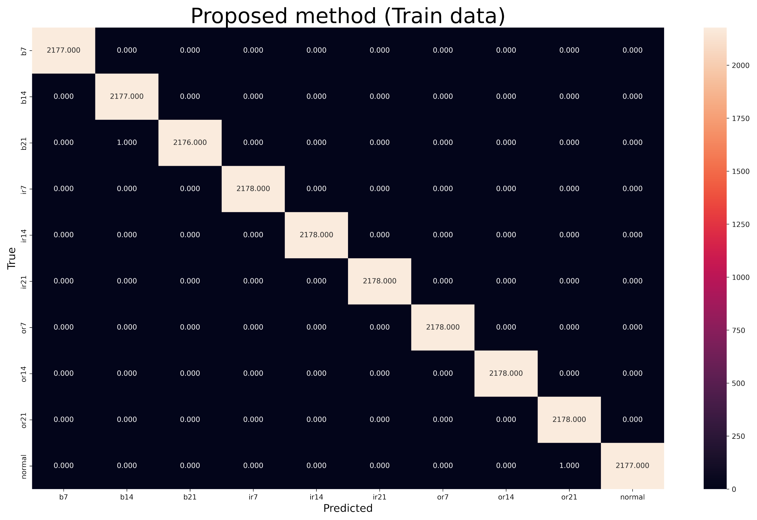
4. CWRU Dataset

The dataset provided by the CWRU [34] Bearing Database is recognized as a standard benchmark for evaluating machine learning models to detect bearing faults. This dataset is available to the public and has been used by many researchers in the field. In this dataset, in addition to the location of the fault, the severity of the fault is also provided.

The dataset used to perform this experiment is the CWRU dataset. Most articles in the field of rotary machine diagnostics have used this dataset, and this will help us to be able to compare the results with other related work.

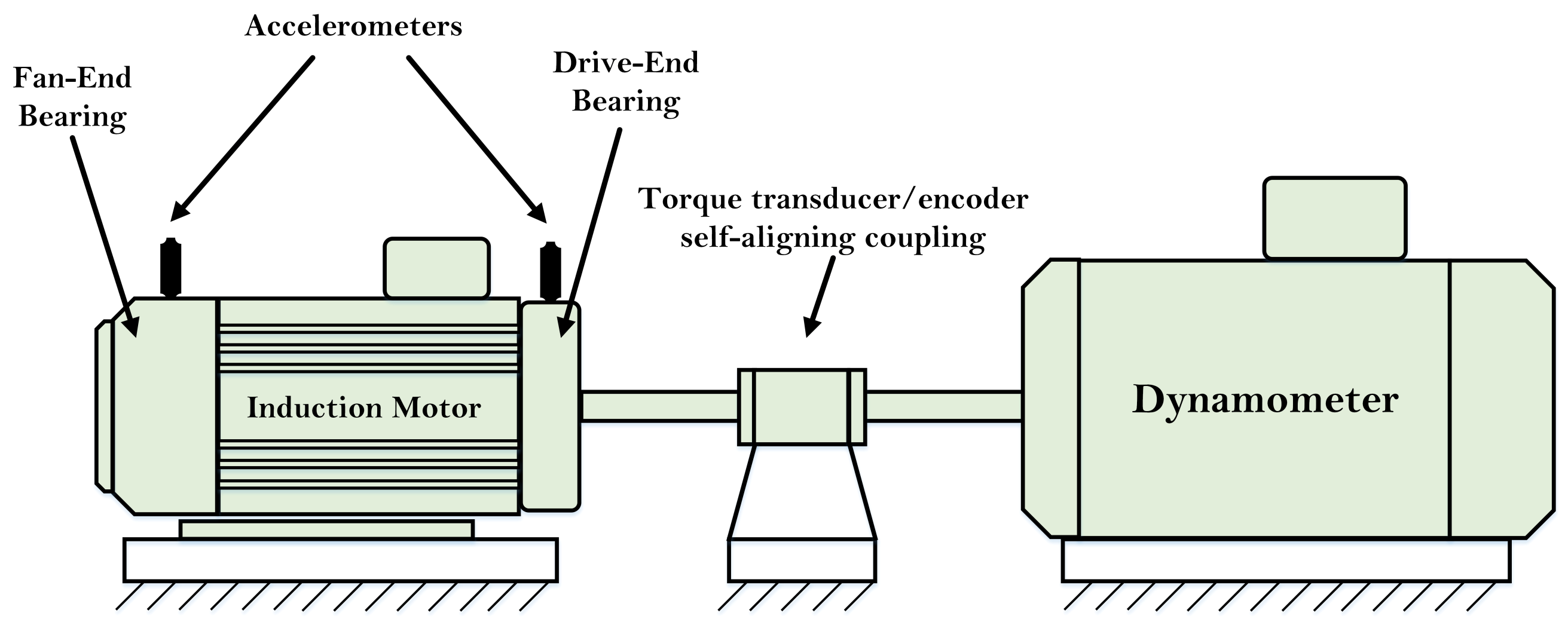
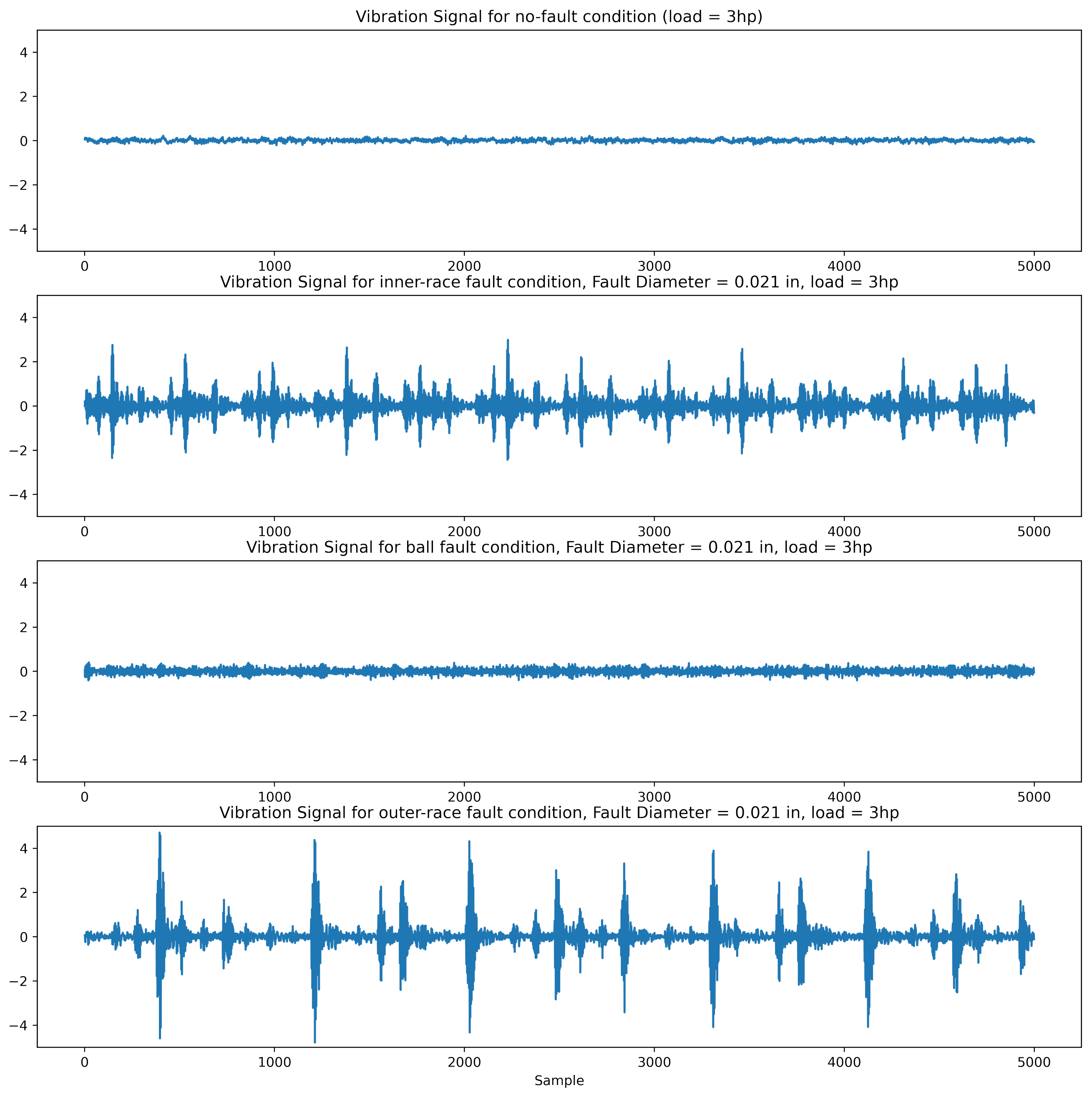
The equipment for this test, shown in Figure 4, consists of a 2 hp motor and a dynamo meter that is used to apply the controlled torque. A torque and encoder transducer is connected to the device to measure the torque and speed, respectively. In addition, three accelerometers are used to obtain the mechanical vibration signal: one on the fan-end bearing, one on the drive-end bearing, and one on the motor holder base. The bearings under test in this dataset are SKF 6205-2RS-Jem bearings, and the data are taken at two sampling rates of 12 KHz and 48 KHz.

The data used in this study are the vibration signal obtained by an accelerometer mounted on the drive end (close to the fault) with a sampling rate of 12 KHz. In this test, the motor rotation speed is changed from 1730 RPM to 1797 RPM and the motor load is changed from 0 and 3 hp to create normal bearing operating conditions. This dataset includes three types of fault that were laboratory-induced by electrical discharge machining (EDM) with a depth of 0.011 inches in different parts of the bearing: the inner raceway, outer raceway, and balls (rolling element). In addition, each fault has three levels, with diameters of 0.007, 0.014, and 0.021 inches. Figure 5 shows a snapshot of these signals.

Considering the healthy state, there are 10 types of data in this dataset in total. The dateset summary is reported in

Table 2. Dataset summary.

Fault Type	Ball			Inner			Outer			Normal
Fault diameter	0.007	0.014	0.021	0.007	0.014	0.021	0.007	0.014	0.021	0
Training	2177	2177	2177	2177	2177	2177	2177	2177	2177	2177
Testing	60	60	60	60	60	60	60	60	60	60
Sample Len.	800	800	800	800	800	800	800	800	800	800
Load (hp)	0, 1, 2, 3	0, 1, 2, 3	0, 1, 2, 3	0, 1, 2, 3	0, 1, 2, 3	0, 1, 2, 3	0, 1, 2, 3	0, 1, 2, 3	0, 1, 2, 3	0, 1, 2, 3
Label	0	1	2	3	4	5	6	7	8	9

. The time window considered in this study includes two complete rotations of the motor shaft. The amount of data in each cycle is obtained by $N=F_s\times 60/\omega$, where $F_s$ is the sampling frequency (Hz), $\omega$ is the motor shaft speed (rpm), and N is the amount of data. The average rotation speed of 1730, 1750, 1772, and 1797 rpm is approximately 1762 and, according to the sampling rate of 12 KHz, there are approximately 400 samples per cycle; two rotations of the motor shaft will give us 800 samples. Therefore, the selected time window will be 800 samples. Seventy-two percent of the data were selected as training, 18% as validation, and 10% as test.

Data Augmentation

Due to the large number of training parameters, deep learning models require large amounts of data for training, but such a dataset is not available. In this study, a data augmentation method called sliding window was used for training data. In this method, instead of creating training data with the size of a time window, the training window is shifted with n time-steps. Therefore, n samples from the previous data are removed and n new samples are added in, where n is the sliding parameter. In this study, $n=200$ was selected and the amount of training data was increased from 5440 to 21,770 samples.

5. Experiments and Results

In this section, the performance of a multi-scale convolutional network model with the proposed bidirectional GRU is investigated. The experiments were performed in 10 repetitions using cross-validation. Each experiment was performed in 30 training iterations with a learning rate of 0.5. Figure 6 shows the convergence speed of the training phase. It is clear that the training error converged rapidly in less than 10 iterations. Sixty test data were provided for each class and no preprocessing was performed on the raw vibration data.

The highest accuracy was 100%, the lowest accuracy was 99.83%, and the average accuracy was 99.96% with a standard deviation of 0.06%. The accuracy of the proposed model for all folds is reported in

Table 3. Accuracy of proposed model.

Fold #	1	2	3	4	5	6	7	8	9	10	Mean (Std)
Accuracy	100%	100%	100%	100%	99.83%	100%	99.83%	100%	100%	100%	99.96 (±0.06)%

.

The confusion matrices for train and test data are depicted in Figure 7 and Figure 8, respectively. It is clear that all the test data were correctly categorized.

In addition, based on

Table 4. Comparison of the proposed scheme with other methods.

Method	No. Classes	Average Testing Accuracy
Time-Frequency Image [11]	4	99.50%
MS-DCNN [23]	10	99.27%
CNN based [12] model	10	99.41%
NSAE-LCN [35]	10	99.92%
SRDCNN [15]	10	99.40%
Deep learning architecture with attention mechanism [14]	10	99.74%
Multi-scale CNN with attention [21]	12	99.86%
ALSCN [36]	7	96.75%
Multi-scale CNN and LSTM [22]	10	98.46%
DCNN [37]	10	98.50%
CNN-BiLSTM [38]	10	98.56%
TST [39]	10	98.63%
Attention stream net [40]	16	99.60%
CRNN [18]	6	99.77%
SR-1DCNN [41]	10	99.82%
Proposed Method	10	99.96%

, it is clear that compared to the other methods, the proposed method achieves higher accuracy.

5.1. Performance in Noisy Conditions

Signals measured in real conditions usually have background noise. In order to evaluate the robustness of the proposed method to the measurement noise, a simulated Gaussian white noise was added to the test data. Then, the model was tested with different values of signal-to-noise ratio. To do this, the power of the vibration signal was calculated and the noise intensity was then calculated in proportion so that the signal-to-noise ratio was obtained. Signal to noise is defined in Equation (20). The $SNR=0$ dB means that the power of the added noise is equal to the power of the input signal.

$$SN{R}_{dB}=10{log}_{10}\left(\frac{P_{signal}}{P_{noise}}\right)$$

(20)

Taking into account all the data, each experiment was performed in 10 iterations without separating the motor speed and the motor load. At each stage, the model was first trained with noise-free data and then evaluated with noisy data. The results of this experiment are provided in

Table 5. Comparison of the accuracy of the proposed model with other methods in the presence of noise with different noise intensities.

Method	SNR
	0 dB	2 dB	4 dB	6 dB	8 dB	10 dB
IMS-FACNN [42]	92.92% ± 0.34	-	97.82% ± 0.26	-	99.39% ± 0.14	-
Multi-scale CNN
and LSTM [22]	81.41% ± 1.15	85.90% ± 1.10	88.19% ± 1.05	90.11% ± 1.09	92.77% ± 1.15	95.25% ± 1.14
MC-CNN [43]	91.33% ± 0.08	95.71% ± 0.17	97.33% ± 0.23	99.61% ± 0.11	-	-
DCNN [37]	87.68%	90.74%	-	93.17%	96.21%	97.77%
WDCNN [44]	71.38%	85.95%	95.21%	98.93%	99.57%	99.67%
SRDCNN [15]	-	95.40%	99.60%	99.60%	99.60%	99.80%
Attention stream
net [40]	-	-	-	-	-	92.74% ± 2.99
Proposed	95.18% ± 1.97	98.58% ± 1.10	99.55% ± 0.36	99.78% ± 0.38	99.85% ± 0.39	99.88% ± 0.14

. According to this table, it is clear that the performance of the proposed method is much better than other methods.

5.1.1. The Effect of Convolution Filter Size under Noise Conditions

As noted in the previous sections, the proposed model has three convolution layers, each of which has filters of a specified size. In this experiment, all hyperparameters were the same, and only the length of the filters changed in each experiment. The signal-to-noise ratio was set to 0dB at all stages. According to

Table 6. The effect of filter size on the performance of the proposed model in noisy conditions.

Filter Size 1, 2, 3	16, 8, 2	32, 16, 4	64, 32, 8	128, 64, 16	256, 128, 32	512, 256, 64
With (SNR 0 dB) noise	56.66%	31.83%	61.66%	75.83%	88.33%	98.83%
Without noise	100%	100%	97.50%	99.83%	99.83%	99.83%
Total parameters	477,482	484,138	448,298	427,770	479,018	487,210

, the results show that more useful features of the vibration signal were extracted under noisy conditions by increasing the length of the convolution filters. It should be noted that although the filter size increased, the number of total parameters was not increased dramatically. This is because of carefully selected pool size in maxpooling $(poolsize=256)$.

5.1.2. The Effect of Pool Size under Noise Conditions

In this experiment, the accuracy of the fault diagnosis under noise conditions iswas evaluated by changing the size of the maxpooling. In all experiments, the signal-to-noise ratio of 0 dB was considered and all parameters were adjusted according to Table 1. This experiment was performed in eight steps, wherein the pool size was selected for all three convolutional layers. The results indicate that with an expanded pooling window, the generalizability of the model increased and had acceptable performance under noise interference. For all experiments, the accuracy for the noise-free data was the same and relatively good.

As the size of the pool increased, due to the reduction of the feature dimensions, the model parameters decreased dramatically. The results of this experiment are reported in

Table 7. The effect of pool size on the performance of the proposed model in noisy conditions.

Pool Size	4	8	16	32	64	128	256
With noise (SNR 0 dB)	82.83%	77.50%	82.16%	83%	85.83%	89.83%	98.83%
Without noise	99.83%	99.66%	99.83%	99.66%	99.83%	99.66%	99.83%
Total parameters	19,509,034	9,875,242	5,058,346	2,649,989	1,371,946	782,122	487,210

.

6. Conclusions

To achieve high accuracy in bearing fault diagnosing even in noisy conditions, a multi-scale CNN + BiGRU was proposed in this study. The proposed method extracts the spatial and temporal features of the various vibration signal on different scales, combines them, and classifies them. The proposed model was evaluated with the CWRU dataset, and the results showed that this method has high accuracy and fast convergence speed. In addition, it was shown that the proposed scheme can obtain important distinguishing features from the raw data without any preprocessing, even in the presence of strong noise. Finally, with noise-free data, the proposed method achieved an average accuracy of 99.96%; with noise-impregnated data, the average accuracy was about 95.18%. In addition, it was proved that, compared to other methods, this scheme can identify the bearing faults with higher accuracy, both in noise-free and noisy conditions. It can be concluded that this model can be used in intelligent fault diagnosis systems for bearings in various applications in industry.