Article

Linear Matrix Inequality Approach to Designing Damping and Tracking Control for Nanopositioning Application

by
Adedayo K. Babarinde
and
Sumeet S. Aphale
*,†
Centre for Applied Dynamics Research, School of Engineering, University of Aberdeen, Aberdeen AB24 3FX, Scotland, UK
*
Author to whom correspondence should be addressed.
These authors contributed equally to this work.
Vibration 2022, 5(4), 846-859; https://doi.org/10.3390/vibration5040050
Submission received: 4 October 2022 / Revised: 15 November 2022 / Accepted: 25 November 2022 / Published: 29 November 2022

Abstract

:
This paper presents a method to extend the eigenstructure assignment based design of the Positive Position Feedback (PPF) damping controller to the family of well-known second-order Positive Feedback Controllers (PFC) namely: (i) the Positive Velocity and Position Feedback (PVPF) and (ii) the Positive Acceleration Velocity and Position Feedback (PAVPF) using appropriate eigenstructure assignment. This design problem entails solving a set of linear equations in the controller parameters using Linear Matrix Inequalities (LMI) to specify a convex design constraint. These damping controllers are popularly used in tandem with a tracking controller (typically an integrator) to deliver high-bandwidth nanopositioning performance. Consequently, the closed-loop performance of all three controllers (PPF, PVPF and PAVPF) employed in tandem with suitably gained integral tracking loops is thoroughly quantified via relevant performance metrics, using measured frequency response data from one axis of a piezo-stack actuated x-y nanopositioner.

1. Introduction

Since the formulation of Positive Position Feedback (PPF) in the early 1990s [1], positive feedback controllers (PFC) have been popularly applied to mitigate vibration problems arising from unwanted excitation of system resonance/s. Soon after Positive Position Feedback (PPF) controller was proposed, the full family of second-order PFC, i.e., Positive Velocity and Position Feedback (PVPF) [2,3], and Positive Acceleration, Velocity and Position Feedback (PAVPF) [4], have also been formalized. These controllers have since found popularity in a number of wide-ranging applications [5,6]. Due to their simplicity, ease of design, relatively good robustness to system parameter uncertainties and excellent stability margins, these controllers are often used in applications where multiple controllers are employed in tandem to deliver on several performance indices, for example: control of nanopositioning systems where damping controllers are implemented (in the inner-loop) to impart adequate damping to the dominant resonant mode of the respective axis; which in turn, facilitates the implementation of high-gain tracking controllers (in the outer-loop) as shown in Figure 1; enabling wide-band, high-precision nanopositioning [7]. In fact, the entire family of second-order PFC damping controllers—PPF, PVPF and PAVPF—have been adopted to enhance positioning performance of nanopositioning systems [4,8]. The PVPF and PAVPF especially when used as standalone controllers (without tracking controllers), have limited capability for reducing closed-loop positioning error and improving bandwidth. However, they exhibit robustness against external disturbances and improved closed loop stability. Though improved strategies to design these PFC-based control schemes have been proposed [9,10,11], they are sub-optimal due to the problem’s non-convex nature. Ref. [12] recently reported a convex PPF controller design using eigenstructure assignment. The stability constraints were found to be Linear Matrix Inequalities (LMIs) in terms of controller parameters. The solution proposed in here was based on the premise that the eigenvalues and eigenvectors of the matrix pencil are matched with that of the desired closed-loop system.
In this work, we extend the formulation as presented in [12], to design PVPF and PAVPF second-order damping controllers. The controllers are designed via convex optimization in relation to solving the related least-squares problems. In addition, necessary and sufficient conditions for the realization of the three positive feedback controllers will be discussed. We compare the closed-loop performances of PPF, PVPF, and PAVPF controllers designed via the proposed eigenstructure assignment over key performance metrics such as 3-dB bandwidth, robustness to resonance frequency shifts, positioning errors and closed-loop disturbance rejection profile. It is envisioned that this design method will facilitate the application of such hybrid (damping and tracking) control strategies to a wider range of positioning systems such as serial link manipulators, ref. [13] and mobile manipulators [14].
The paper is structured as follows: Section 2 provides an overview of the notations and identities used for each of the controller. The overview of controller design is presented in Section 3, while the realization of the controller is presented in Section 3.2. Section 4 gives the comparative closed-loop performance evaluation and results. Finally, Section 5 concludes the paper.

2. Preliminary Definitions

The preliminary definitions related to quadratic eigenvalue and eigenvector assignment problem are defined in [12]. For continuity and completeness, they are briefly included below. A second-order mass-spring-damper model is given in (1).
x ¨ + 1 x ˙ + 2 x = Ψ T u y = Ψ x
where 1 and 2 are damping and stiffness matrix, Ψ is the input matrix, while y ( t ) and x ( t ) are the output vector and state vector, respectively. Similarly, the structure of the popular PPF controller is given by:
z ¨ + D 1 z ˙ + D 2 z = Γ 0 y u = Γ 0 z
where z ( t ) is the controller state and, D 1 , D 2 and Γ 0 are controller parameters of appropriate size to match the system matrices given in (1). Then, these controller parameters are designed such that the closed-loop system given by
x ¨ z ¨ + 1 0 0 D 1 x ˙ z ˙ + 2 Ψ T Γ 0 Γ 0 T Ψ D 2 x z = 0
Theorem III.1. in [12] then details the method of employing eigen-structure matching technique in solving for the optimal PPF Controller. The goal of this exercise then is to match the eigenvalues and eigenvectors of the matrix pencil given in (4), to be matched with the desired closed-loop system whose block diagram is shown in Figure 1.
P ( λ ) = λ 2 + λ K 1 + K 2
where K 1 and K 2 are positive definite.
In the following section, the same framework will be employed to first design the PPF controller and the integral gain associated with it. Noting that PVPF and PAVPF controllers can be realized by progressively adding one (for PVPF) and two (for PAVPF) more terms to the PPF design framework, these two controllers are designed.

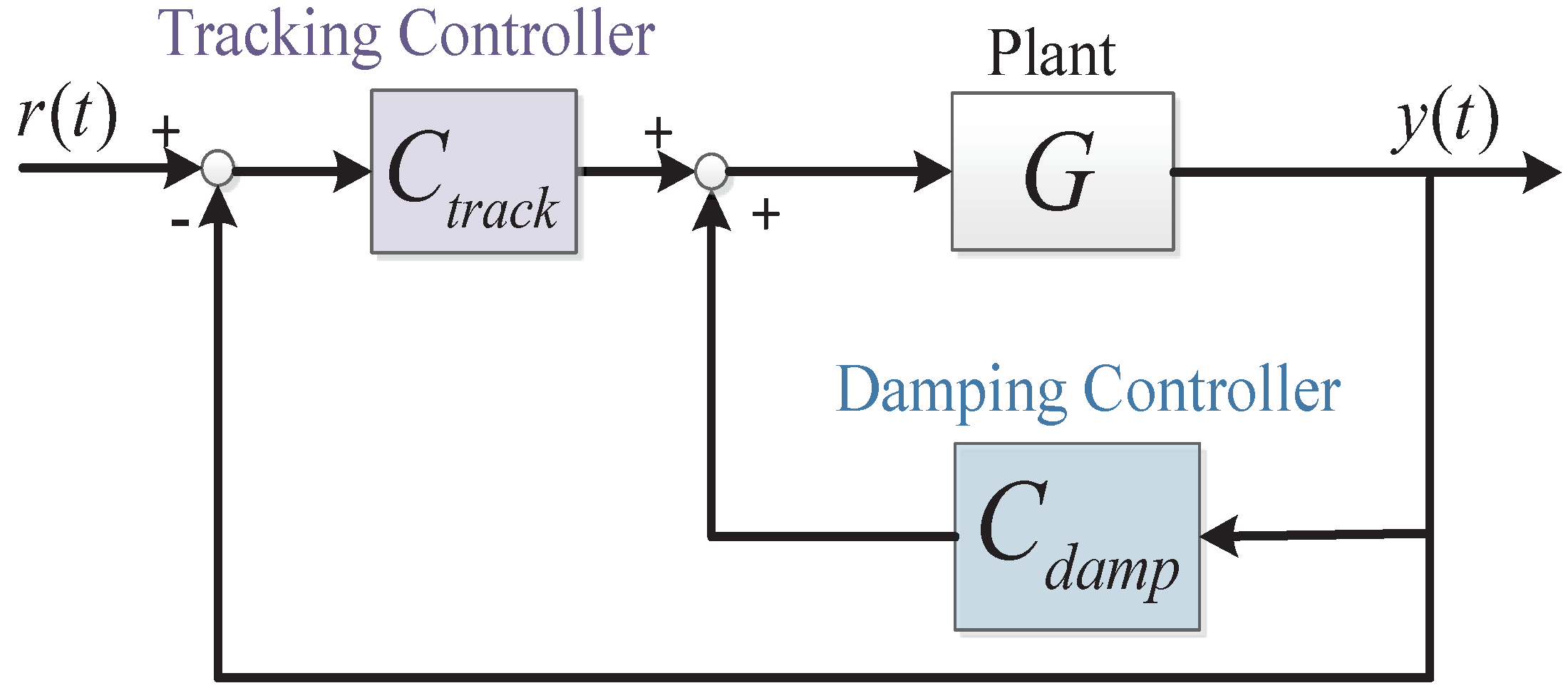
3. Controller Design

As presented in [12], considering the second-order plant in (1), the PPF controller is designed such that the closed-loop system depicted in Figure 1 is given by
x ¨ z ¨ + 1 0 0 D 1 x ˙ z ˙ + 2 Ψ T Γ 0 Γ 0 T Ψ D 2 x z = 0
As depicted in Figure 1, we introduce an integral tracking controller given by
C t r a c k ( s ) = k t s
Consequently, the PVPF and PAVPF designs in closed-loop can be formulated respectively as:
x ¨ z ¨ + 1 0 Γ 0 Ψ D 1 x ˙ z ˙ + 2 Ψ T Γ 1 Ψ D 2 x z = 0
and
x ¨ z ¨ + 1 w f 0 Γ 0 Ψ D 1 x ˙ z ˙ + 2 w f Ψ T Γ 1 Ψ D 2 x z + 2 w f 0 Γ 2 Ψ D 2 x z = 0
where D 1 , D 2 , and Γ 0 , Γ 1 and Γ 2 are design parameters. The design then simplifies to matching these to a second-order system with the desired damping as stated in (9).
p ¨ + K 1 p ˙ + K 2 p

3.1. PPF Controller Design

For continuity and completeness, the PPF controller design is repeated here as presented in [12]. Thus, the PPF controller design can be realized if the linear Equation (9) has a solution.
A κ = β
where
A = [ ( Λ T W T I ) P 1 ( W T I ) P 2
P 1 = v e c 0 0 0 T 1 v e c 0 0 0 T 1 = 0 P 2 = v e c ( Γ 1 ) v e c ( Γ 2 ) v e c ( Γ m p ) v e c ( P 1 ) Γ k = 0 Ψ T B k B T Ψ 0 α = v e c 1 D 1 v e c 1 Γ , D 2
β = v e c W Λ 2 Λ T W T I v e c 1 0 0 0 W T I v e c 0 0 0
Λ and W are the eigenvalue-eigenvector matrices satisfying (6).
Hence, we match the closed-loop system in (6) with the second-order reference system in (9) by ensuring that the eigenvalues and eigenvectors of (5) are equal to that of the closed-loop system of (6).
W Λ 2 + 1 0 Γ 1 ρ D 1 x ˙ t ˙ W Λ + 2 Ψ T Γ 2 Ψ D 2 W = 0
Then, the linear system of equations in (13) can be solved as follows:
Let E n denote the linear subspace of all n × n symmetrical matrices with dimension n ( n + 1 ) 2 Then we represent the standardized basis of E n by
B = T 1 , T 2 , , T n ( n + 1 ) 2
Step 1: Considering both D 1 , D 2 E p , they can be expressed as a set linear combination with respect to the standardized basis as depicted in (15).
D i = k = 1 p ( p + 1 ) 2 d k i T k , i = 1 , 2 .
Similarly, the matrix Γ is written as a combination of the standard basis of R m × n
Γ = k = 1 m p μ k B k .
putting (16) and (17) into (6) yields
1 0 0 D 1 = 1 0 0 0 + k = 1 p ( p + 1 ) 2 d k 1 0 0 0 T k
1 Ψ T Γ 0 D 2 = 2 0 0 0 + k = 1 p ( p + 1 ) 2 d k 2 0 0 0 T k + k = 1 m p μ k 0 Ψ T B k B k T Ψ 0
From the (14)–(18), the unknowns d k 1 , d k 2 and μ k k = 1 m p are unknowns.
Step 2: We derive expressions for the vectorization of (15) and use it to develop sets of linear equations for the unknowns in (15)–(19).
v e c 1 0 0 D 1 W Λ = Λ T W T I v e c 1 0 0 D 1 = Λ T W T I v e c 1 0 0 0 + k = 1 p ( p + 1 ) 2 d k 1 0 0 0 T k = Λ T W T I P 1 v e c 1 v e c 1 0 0 0
where
P 1 = v e c 0 0 0 T 1 v e c 0 0 0 T p ( p + 1 ) 2
Likewise,
v e c 2 Ψ T Γ Γ T Ψ D 2 W Λ = W T I v e c 2 T Γ Γ T Ψ D 2 = W T I P 2 v e c 1 ( Γ , D 2 ) v e c 2 0 0 0
where
P 2 = v e c Γ 1 v e c Γ v e c Γ m p v e c P 1
with
Γ k = 0 Ψ T B k B k T Ψ 0
Step 3: The sets of expression derived in step 2 are used to regenerate the (13) in vectorized form.
v e c 1 0 0 D 1 W Λ + v e c 2 Ψ T Γ Γ T Ψ D 2 W = v e c W Λ 2
Putting (20) and (22) in (25) and rearranging yields the following equation
Λ T W T I P 1 v e c 1 D 1 + W T I P 2 v e c 1 Γ , D 2 = v e c W Λ 2 Λ T W T I v e c 1 0 0 0 W T I v e c 2 0 0 0
as in Equations (11)–(13) respectively.

3.2. PVPF and PAVPF Controller Design

The PVPF and PAVPF controller design are implemented as follows;
PVPF Controller Design: The PVPF controller is realized if the linear equation Equation (9) has a solution. Like the case of PPF controller, we consider (10) and (11), hence we realize the PVPF controller design as follows;
P 1 = v e c 0 0 0 T 1 v e c 0 0 0 T 1 = 0 P 2 = v e c ( Γ 1 ) v e c ( Γ 2 ) v e c ( Γ m p ) v e c ( P 1 ) Γ k = 0 Ψ T B k B T Ψ 0 α = v e c 1 D 1 v e c 1 Γ , Γ 1 , D 2
β = v e c W Λ 2 Λ T W T I v e c 1 Γ 1 Γ 1 0 W T I v e c 0 0 0
Λ and W are the eigenvalue-eigenvector matrices satisfying (6).
Hence, we match the closed-loop system in (6) with the second-order reference system in (9) by ensuring that the eigenvalues and eigenvectors of (5) are equal to that of the closed-loop system of (6).
W Λ 2 + 1 0 Γ 1 ρ D 1 x ˙ t ˙ W Λ + 2 Ψ T Γ 2 Ψ D 2 W = 0
Then, the linear system of equations in (13) can be solved as follows:
Let E n denote the linear subspace of all n × n symmetrical matrices with dimension n ( n + 1 ) 2 Then we represent the standardized basis of E n by
B = T 1 , T 2 , , T n ( n + 1 ) 2
Step 1: Considering both D 1 , D 2 E p , they can be expressed as a set linear combination with respect to the standardized basis as depicted in (30).
D i = k = 1 p ( p + 1 ) 2 d k i T k , i = 1 , 2 .
Similarly, the matrix Γ is written as a combination of the standard basis of R m × n
Γ = k = 1 m p μ k B k .
putting (31) and (32) into (6) yields
1 Γ 1 Γ 1 D 1 = 1 Γ 1 Γ 1 0 + k = 1 p ( p + 1 ) 2 d k 1 0 0 0 T k
1 Ψ T Γ 0 D 2 = 2 0 0 0 + k = 1 p ( p + 1 ) 2 d k 2 0 0 0 T k + k = 1 m p μ k 0 Ψ T B k B k T Ψ 0
From the (29)–(33), the unknowns d k 1 , d k 2 and μ k k = 1 m p are unknowns.
Step 2: We derive expressions for the vectorization of (30) and use it to develop sets of linear equations for the unknowns in (30)–(34).
v e c 1 Γ 1 Γ 1 D 1 W Λ = Λ T W T I v e c 1 Γ 1 Γ 1 D 1 = Λ T W T I v e c 1 Γ 1 Γ 1 0 + k = 1 p ( p + 1 ) 2 d k 1 0 0 0 T k = Λ T W T I P 1 v e c 1 v e c 1 Γ 1 Γ 1 0
where
P 1 = v e c 0 0 0 T 1 v e c 0 0 0 T p ( p + 1 ) 2
Likewise,
v e c 2 Ψ T Γ Γ T Ψ D 2 W Λ = W T I v e c 2 T Γ Γ T Ψ D 2 = W T I P 2 v e c 1 ( Γ , Γ 1 , D 2 ) v e c 2 Γ 1 Γ 1 0
where
P 2 = v e c Γ 1 v e c Γ v e c Γ m p v e c P 1
with
Γ k = 0 Ψ T B k B k T Ψ 0
Step 3: The sets of expression derived in step 2 are used to regenerate the (13) in vectorized form.
v e c 1 Γ 1 Γ 1 D 1 W Λ + v e c 2 Ψ T Γ Γ T Ψ D 2 W = v e c W Λ 2
Putting (35) and (37) in (40) and rearranging yields the following equation
Λ T W T I P 1 v e c 1 D 1 + W T I P 2 v e c 1 Γ , D 2 = v e c W Λ 2 Λ T W T I v e c 1 Γ 1 Γ 1 0 W T I v e c 2 0 0 0
With the conditions in Section 2, the PVPF controller is realizable if and only if (10) has a solution. If (10) has infinite solutions, then the convex optimal PVPF controller could be obtained by solving
min κ | | A κ β | | w 2 + λ | | Γ 2 | | w 2 + λ | | Γ 1 | | w 2 , λ > 0
PAVPF Controller Design: The PAVPF controller is realized if the linear equation Equation (9) has a solution. Like the case of PPF controller, we consider (10) and (11), hence we realize the PAVPF controller design as follows;
P 1 = v e c 0 0 0 T 1 v e c 0 0 0 T 1 = 0 P 2 = v e c ( Γ ) v e c ( Γ 1 ) v e c ( Γ 2 ) v e c ( Γ m p ) v e c ( P 1 ) Γ k = 0 Ψ T B k B T Ψ 0 α = v e c 1 D 1 v e c 1 Γ , Γ 1 , Γ 2 , D 2
β = v e c W Λ 2 Λ T W T I v e c 1 Γ 1 Γ 1 0 W T I v e c 0 0 0
Λ and W are the eigenvalue-eigenvector matrices satisfying (6).
Hence, we match the closed-loop system in (6) with the second-order reference system in (9) by ensuring that the eigenvalues and eigenvectors of (5) are equal to that of the closed-loop system of (6).
W Λ 2 + 1 0 Γ 1 ρ D 1 x ˙ t ˙ W Λ + 2 Ψ T Γ 2 Ψ D 2 W = 0
Then, the linear system of equations in (13) can be solved as follows:
Let E n denote the linear subspace of all n × n symmetrical matrices with dimension n ( n + 1 ) 2 Then we represent the standardized basis of E n by
B = T 1 , T 2 , , T n ( n + 1 ) 2
Step 1: Considering both D 1 , D 2 E p , they can be expressed as a set linear combination with respect to the standardized basis as depicted in (46).
D i = k = 1 p ( p + 1 ) 2 d k i T k , i = 1 , 2 .
Similarly, the matrix Γ is written as a combination of the standard basis of R m × n
Γ = k = 1 m p μ k B k .
putting (47) and (48) into (6) yields
1 Γ 1 Γ 1 D 1 = 1 Γ 1 Γ 1 0 + k = 1 p ( p + 1 ) 2 d k 1 0 0 0 T k
1 Ψ T Γ 0 D 2 = 2 0 0 0 + k = 1 p ( p + 1 ) 2 d k 2 0 0 0 T k + k = 1 m p μ k 0 Ψ T B k B k T Ψ 0
From the (45)–(49), the unknowns d k 1 , d k 2 and μ k k = 1 m p are unknowns.
Step 2: We derive expressions for the vectorization of (46) and use it to develop sets of linear equations for the unknowns in (46)–(50).
v e c 1 Γ 1 Γ 1 D 1 W Λ = Λ T W T I v e c 1 Γ 1 Γ 1 D 1 = Λ T W T I v e c 1 Γ 1 Γ 1 0 + k = 1 p ( p + 1 ) 2 d k 1 0 0 0 T k = Λ T W T I P 1 v e c 1 v e c 1 Γ 1 Γ 1 0
where
P 1 = v e c 0 0 0 T 1 v e c 0 0 0 T p ( p + 1 ) 2
Likewise,
v e c 2 Ψ T Γ Γ T Ψ D 2 W Λ = W T I v e c 2 T Γ Γ T Ψ D 2 = W T I P 2 v e c 1 ( Γ , Γ 1 , Γ 2 , D 2 ) v e c 2 Γ 1 Γ 1 0
where
P 2 = v e c Γ 2 v e c Γ 1 v e c Γ v e c Γ m p v e c P 1
with
Γ k = 0 Ψ T B k B k T Ψ 0
Step 3: The sets of expression derived in step 2 are used to regenerate the (13) in vectorized form.
v e c 1 Γ 1 Γ 1 D 1 W Λ + v e c 2 Ψ T Γ Γ T Ψ D 2 W = v e c W Λ 2
Putting (51) and (53) in (56) and rearranging yields the following equation
Λ T W T I P 1 v e c 1 D 1 + W T I P 2 v e c 1 Γ , D 2 = v e c W Λ 2 Λ T W T I v e c 1 Γ 1 Γ 1 0 W T I v e c 2 Γ 2 Γ 2 0
With the conditions in Section 2, the PAVPF controller is realizable if and only if (10) has a solution. If (10) has infinite solutions, then the convex optimal PAVPF controller could be obtained by solving
min κ | | A κ β | | w 2 + λ | | Γ 2 | | w 2 + λ | | Γ 1 | | w 2 + λ | | Γ | | w 2 , λ > 0
subject to
1 0 Γ 1 ρ D 1 = κ 1 I
2 ρ T Γ 2 ρ D 2 = κ 2 I
where I is an identity matrix, w is the positive definite weighting matrix, and κ 1 and κ 2 are positive scalars. The Linear Matrix Inequality constraints in (58)–(60) impose stability on both the controller and closed loop system.
It should be noted that the damping is achieved by the Positive feedback controllers (PPF, PVPF, and PAVPF), and tracking was achieved using the integral controller. The gain of the integrator was selected numerically to deliver a maximum −3 dB bandwidth. The resulting controllers are presented in Table 1.

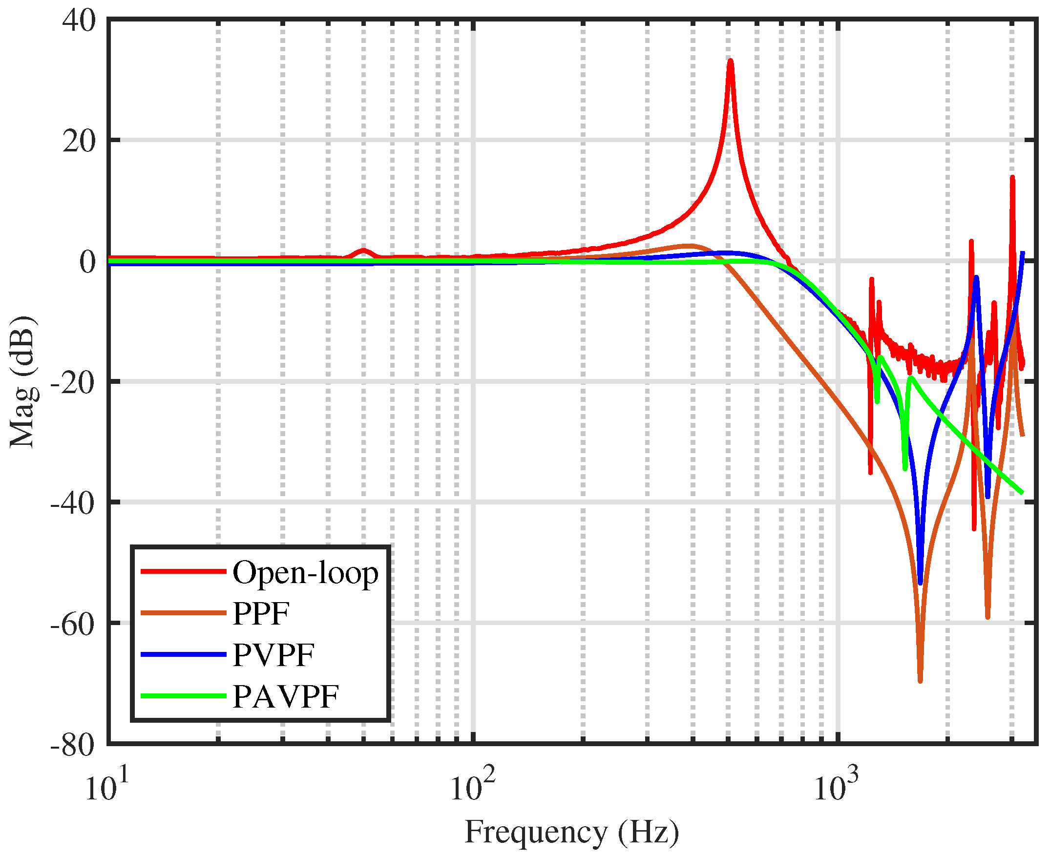
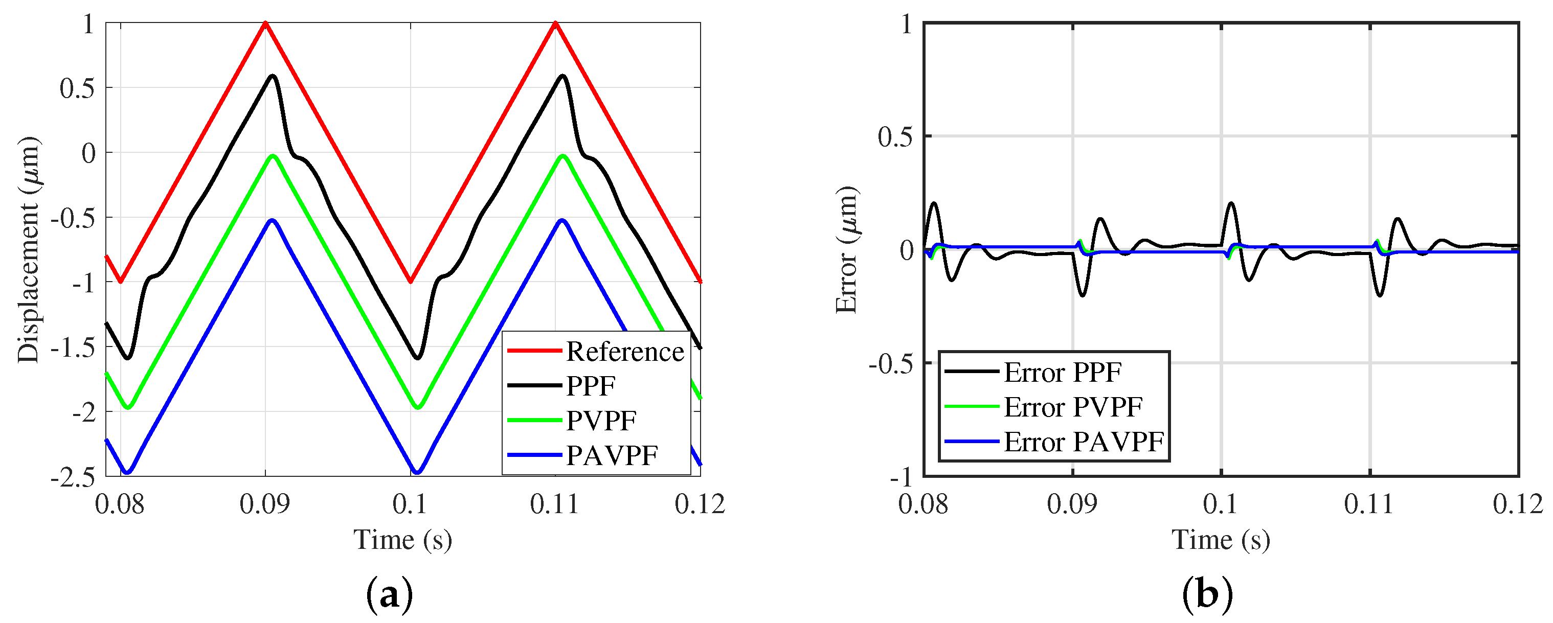
4. Comparative Closed-Loop Performance Evaluation

The closed-loop performance evaluation is obtained by conducting a battery of comparative, closed-loop simulated experiments using the frequency response data recorded on a serial-kinematic nanopositioner as described in [11]. The performance metrics employed are: (a) 3-dB bandwidth, (b) Robustness to resonance frequency shifts, (c) Disturbance rejection profile and (d) Positioning error.

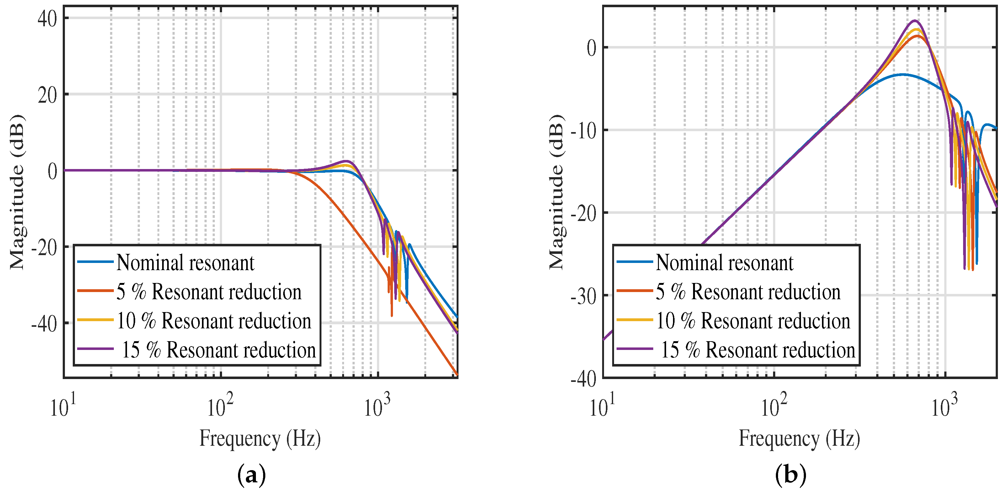
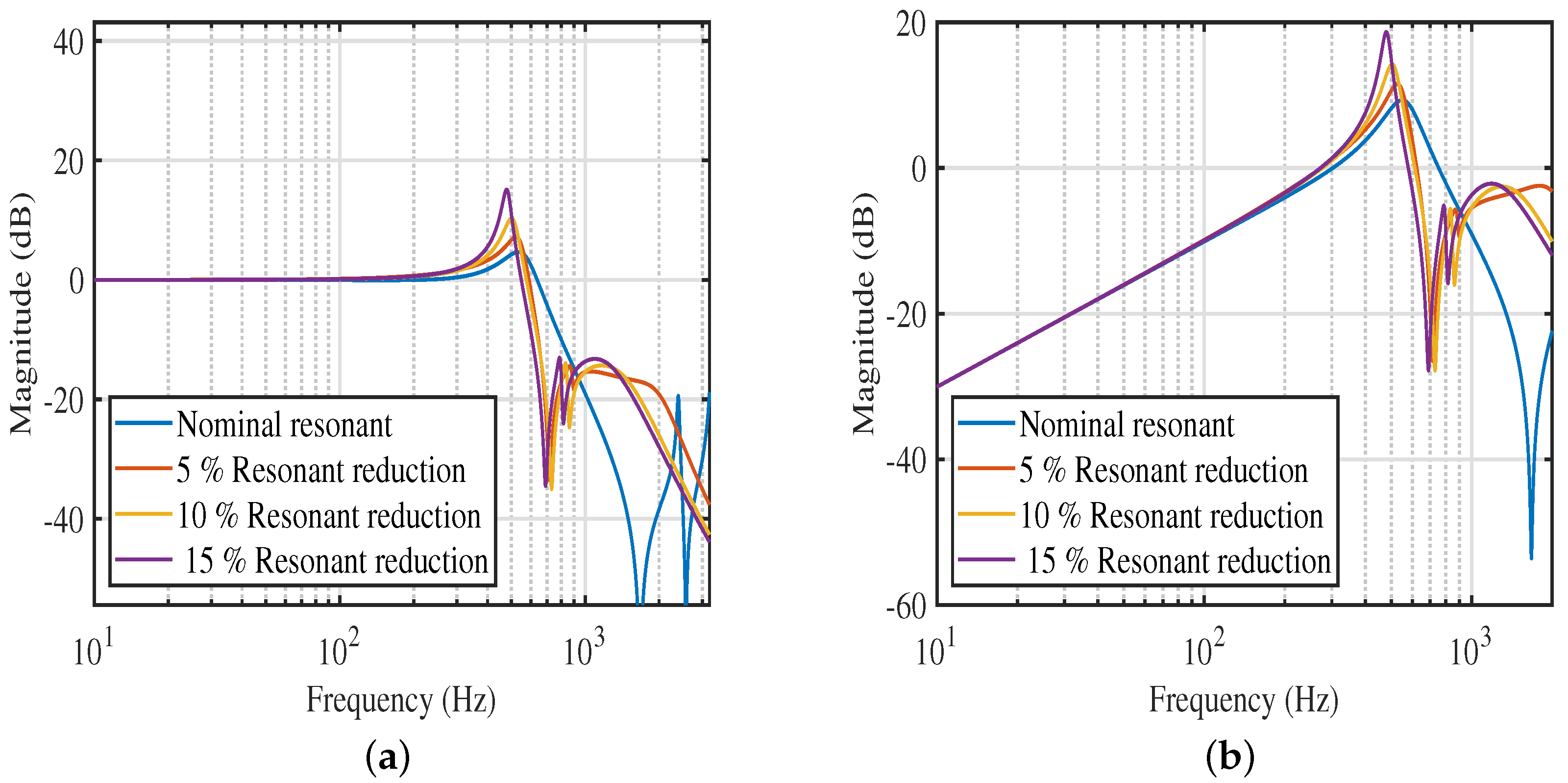
Closed-Loop Analysis against Frequency-Domain Performance Metrics

The 3-dB bandwidth criteria is a popular metric used for assessing the tracking/positioning performance of nanopositioning platforms/systems. Using the method described in Section 3, the open-loop magnitude response and closed-loop magnitude responses for the proposed PPF, PVPF, and PAVPF system using eigenstructure assignment were plotted, as shown in Figure 2. It is evident that the three damping controllers are capable of imparting adequate damping to the resonant mode of the nanopositioner and, with the corresponding integral tracking controllers, achieve significant closed-loop 3-dB bandwidth see Table 1. It can also be seen that the PAVPF + I strategy achieves the highest 3-dB bandwidth of 808 Hz. This is not a significant improvement from the 805 Hz achieved by the PVPF + I strategy but an upgrade to the 536 Hz achieved by the PPF + I strategy.
In addition, the PAVPF + I outperforms the other strategies in terms of robustness to resonant frequency shifts. Nanopositioners undergo variation in loading due to the tasks they perform or the specimens they are aimed to move during scanning applications. These load changes introduce changes in resonance frequencies. As seen in Figure 3, this is where the PAVPF + I excels. As can be seen, for successive reductions in resonance frequency, the PAVPF + I scheme (Figure 3a) has a more graceful performance degradation, while the PVPF + I scheme (Figure 4a) is the worst of the three. The disturbance rejection profiles are plotted in Figure 3b, Figure 4b and Figure 5b. At a cursory glance, it looks like the PPF + I scheme (Figure 5b) is the best of the three, never once breaching the 0 dB line. On the other hand, the PAVPF + I (Figure 3b) does breach the 0 dB line ever so slightly, especially at 10% and 15% resonance frequency shifts. Nevertheless, it is also apparent that the PPF + I shows significant amplification of noise magnitudes at the higher (uncontrolled) resonant modes. In contrast, the PAVPF + I show no increase in noise sensitivity at these frequencies. The PVPF + I show the worst noise sensitivity performance. Consequently, the PAVPF + I scheme emerges as the best-performing in the frequency domain metrics.
The time-domain positioning performance of nanopositioning systems is popularly analyzed for triangular signal inputs as they are wide-band signals and are employed to generate raster patterns used in many scanning applications. Consequently, the time-domain performance of each control scheme is assessed for triangular trajectories with fundamental frequencies of 35 Hz and 50 Hz, respectively. The tracking results and associated errors are presented in Figure 6 and Figure 7. The error trajectories as presented in Figure 6 and Figure 7b have two components: (i) the constant bias that makes the plots look like rectangular pulses—due to the closed-loop system’s phase shift and (ii) the damped ripple riding on the rectangular pulse—the actual positioning error due to tracking mismatch at individual harmonic components that make up the triangular trajectory. Note that the triangle wave is an infinite-bandwidth signal while the closed-loop system and the ADC/ DAC associated with any such experiments are band-limited. Therefore, to make a fair comparison of the positioning performance over a significant bandwidth, both RMS error and Maximum error trends for all three control schemes were simulated and plotted in Figure 8. It is clear that the PAVPF + I and PVPF + I control scheme delivers significantly improved positioning performance, especially for higher frequency trajectories.

5. Conclusions

This paper successfully extended the eigenstructure assignment-based design method to design the full family of Positive Feedback Controllers aimed at damping augmentation, namely—(i) the Positive Velocity and Position Feedback (PVPF) and (ii) the Positive Acceleration Velocity and Position Feedback (PAVPF). The three controllers were then used in tandem with suitably gained integral tracking controllers, and their efficacy in improving the positioning performance of a piezo-actuated nanopositioner was quantified via well-known performance metrics both in the time- and frequency domain. The detailed analysis suggests that the PAVPF + I scheme is the best overall control scheme for such nanopositioners, while the PVPF + I comes in second. The PPF + I show the worst performance of the three. However, when aiming for high-speed nanopositioning (tracking trajectories with a higher fundamental frequency), the PAVPF + I outperforms the other two by a considerable margin. Due to the uniqueness of the proposed methods, their application is ideal for improving the performance of precise high-speed nanopositioning systems. Future work will aim at automating the control design and optimization combined with online estimation of the system model.

Author Contributions

A.K.B., software, investigation, data curation, writing—orginal draft; S.S.A., methodology, validation, writing—review and editing, supervision. All authors have read and agreed to the published version of the manuscript.

Funding

This research received no external funding.

Institutional Review Board Statement

Not applicable.

Informed Consent Statement

Not applicable.

Data Availability Statement

Not applicable.

Conflicts of Interest

The authors declare no conflict of interest.

References

  1. Fanson, J.L.; Caughey, T.K. Positive position feedback control for large space structures. AIAA J. 1990, 28, 717–723. [Google Scholar] [CrossRef]
  2. Bhikkaji, B.; Ratnam, M.; Fleming, A.J.; Moheimani, S.O.R. High-performance control of piezoelectric tube scanners. IEEE Trans. Control Syst. Technol. 2007, 15, 853–866. [Google Scholar] [CrossRef]
  3. Tao, Y.; Li, L.; Li, H.; Zhu, L. High-Bandwidth Tracking Control of Piezoactuated Nanopositioning Stages via Active Modal Control. IEEE Trans. Autom. Sci. Eng. 2021, 19, 2998–3006. [Google Scholar] [CrossRef]
  4. Li, L.; Li, C.X.; Gu, G.; Zhu, L.M. Positive acceleration, velocity and position feedback based damping control approach for piezo-actuated nanopositioning stages. Mechatronics 2017, 47, 97–104. [Google Scholar] [CrossRef]
  5. Syed, H.H. Comparative study between positive position feedback and negative derivative feedback for vibration control of a flexible arm featuring piezoelectric actuator. Int. J. Adv. Robot. Syst. 2017, 14, 1729881417718801. [Google Scholar] [CrossRef] [Green Version]
  6. Liu, Y.; Chen, H. Adaptive sliding mode control for uncertain active suspension systems with prescribed performance. IEEE Trans. Syst. Man Cybern. Syst. 2020, 51, 6414–6422. [Google Scholar] [CrossRef]
  7. Devasia, S.; Eleftheriou, E.; Moheimani, S.O.R. Survey of Control Issues in Nanopositioning. IEEE Trans. Control. Syst. Technol. 2007, 15, 802–823. [Google Scholar] [CrossRef]
  8. Aphale, S.S.; Bhikkaji, B.; Moheimani, S.O.R. Minimizing scanning errors in piezoelectric stack-actuated nanopositioning platforms. IEEE Trans. Nanotechnol. 2008, 7, 79–90. [Google Scholar] [CrossRef]
  9. Wang, X.; Li, L.; Zhu, Z.; Zhu, L. Simultaneous damping and tracking control of a normal-stressed electromagnetic actuated nanopositioning stage. Sens. Actuators Phys. 2022, 338, 113467. [Google Scholar] [CrossRef]
  10. Russell, D.; Fleming, A.J.; Aphale, S.S. Simultaneous Optimization of Damping and Tracking Controller Parameters Via Selective Pole Placement for Enhanced Positioning Bandwidth of Nanopositioners. ASME 2015, 137, 101004. [Google Scholar] [CrossRef]
  11. Babarinde, A.K.; Li, L.; Zhu, L.; Aphale, S.S. Experimental validation of the simultaneous damping and tracking controller design strategy for high-bandwidth nanopositioning—A PAVPF approach. IET Control Theory Appl. 2020, 14, 3506–3514. [Google Scholar] [CrossRef]
  12. Visalakshi, V.; Khare, S.; Moheimani, S.O.R.; Bhikkaji, B. Design of Positive Position Feedback Controllers for Collocated Systems. In Proceedings of the American Control Conference (ACC), Atlanta, GA, USA, 25–28 May 2021; pp. 4791–4796. [Google Scholar]
  13. Mahmoud Abdallah, M.; Fareh, R. Fractional order active disturbance rejection control for trajectory tracking for 4-DOF serial link manipulator. Int. J. Model. Identif. Control. 2020, 36, 57–65. [Google Scholar] [CrossRef]
  14. Algrnaodi, M.M.; Maarouf Saad, M.; Saad, M.; Fareh, R.; Brahmi, A. Trajectory tracking for mobile manipulator based on nonlinear active disturbance rejection control. Int. J. Model. Identif. Control 2021, 37, 95–105. [Google Scholar] [CrossRef]
Figure 1. Block diagram of the traditional dual-loop damping and tracking control scheme employed in precision positioning applications. In the context of this work, the damping controller is one of PPF/ PVPF/ PAVPF family and the tracking controller is an adequately gained integrator.
Vibration 05 00050 g001
Figure 2. The comparison of magnitude responses of the systems in open-loop and closed-loop under the proposed PPF, PVPF and PAVPF controllers using Eigenvector method.
Vibration 05 00050 g002
Figure 3. (a) Closed-loop magnitude response under resonant frequency changes for PAVPF scheme; (b) Disturbance rejection profile for various resonant frequency changes for PAVPF scheme.
Vibration 05 00050 g003
Figure 4. (a) Closed-loop magnitude response under resonant frequency changes for PVPF scheme; (b) Disturbance rejection profile for various resonant frequency changes for PVPF scheme.
Vibration 05 00050 g004
Figure 5. (a) Closed-loop magnitude response under resonant frequency changes for PPF scheme; (b) Disturbance rejection profile for various resonant frequency changes for PPF scheme.
Vibration 05 00050 g005
Figure 6. (a) Time domain traces by the proposed PPF, PVPF and PAVPF controllers for 35 Hz triangular wave input; (b) Measured error by proposed PPF, PVPF and PAVPF controller for 35 Hz triangular wave input.
Vibration 05 00050 g006
Figure 7. (a) Time domain traces by the proposed PPF, PVPF and PAVPF controllers for 50 Hz triangular wave input; (b) Measured error by proposed PPF, PVPF and PAVPF controller for 50 Hz triangular wave input.
Vibration 05 00050 g007
Figure 8. RMS error (a) and Maximum error (b) trends while tracking triangular trajectories of fundamental frequencies ranging from 5 Hz to 50 Hz and a displacement range of ±1 μ m for PPF + I, PVPF + I and PAVPF + I schemes designed using the presented eigenstructure assignment method.
Vibration 05 00050 g008
Table 1. Controller transfer function.
ControllerDampingTracking ± 3 dB Bandwidth (Hz)
PPF + I C d ( s ) = 5.5 × 10 7 s 2 + 1.173 × 10 4 s + 9.856 × 10 7 C t ( s ) = 1620 s 536
PVPF + I C d ( s ) = 9.48 × 10 4 s 4.743 × 10 7 s 2 + 2.929 × 10 4 s + 3.588 × 10 8 C t ( s ) = 1800 s 805
PAVPF + I C d ( s ) = 600 s 2 2.05 × 10 7 s + 4.418 × 1 0 10 s 2 + 1.845 × 10 6 s + 4.83 × 1 0 10 C t ( s ) = 3050 s 808
Publisher’s Note: MDPI stays neutral with regard to jurisdictional claims in published maps and institutional affiliations.

