Influence of Voltage, Pulselength and Presence of a Reverse Polarized Pulse on an Argon–Gold Plasma during a High-Power Impulse Magnetron Sputtering Process

Abstract

This work aims to provide information about the deposition of gold via bipolar high-power impulse magnetron sputtering (HIPIMS) in order to identify suitable process parameters. The influences of voltage, pulse length and the kick-pulse on an argon–gold plasma during a bipolar high-power impulse magnetron sputtering deposition process were analysed via optical emission spectroscopy (OES) and oscilloscope. The voltage was varied between 700 V and 1000 V, the pulse length was varied between 20 µs and 100 µs and the process was observed once with kick-pulse and once without. The influence of the voltage on the plasma was more pronounced than the influence of the pulse width. While the intensity of several Au I lines increased up to 13-fold with increasing voltages, only a less-than linear increase in Au I brightness with time could be identified for changes in pulse length. The intensity of excited argon is only minimally affected by changes in voltages, but follows the evolution of the discharge current, with increasing pulse lengths. Contrary to the excited argon, the intensity emitted by ionized argon grows nearly linearly with voltage and pulse length. The reverse polarised pulse mainly affects the excited argon atoms in the plasma, while the influence on the ionized argon is less pronounced, as can be seen in the the spectra. Unlike the excited argon atoms, the excited gold atoms appear to be completely unaffected by the kick-pulse. No ionization of gold was observed. During the pulse, a strong rarefaction of plasma takes place. Very short pulses of less than 50 µs and high voltages of about 1000 V are to be preferred for the deposition of gold layers. This paper offers a comprehensive overview of the gold spectrum during a HIPIMS process and makes use of optical emission spectroscopy as a simple measuring approach for evaluation of the reverse polarized pulse during a bipolar process. Future uses of the process may include the metallization of polymers.

1. Introduction

1.1. High-Power Impulse Magnetron Sputtering (HIPIMS)

Low-temperature plasmas find a lot of applications in various fields. Non-thermal plasma, atmospheric plasma and physical vapour deposition (PVD) are several examples. An overview of actual applications of plasma in areas such as medicine, agriculture, added manufacturing or propulsion in space can be found in [1]. Non-thermal plasmas have found various biomedical and environmental applications [2]. PVD encompasses various processes like DC-PVD, RF-PVD or HIPIMS. The last one mentioned, HIPIMS, is a relatively new PVD process that was described by Kouznetsov in 1999 [3]. There have been several works that laid the foundation for the process, one of them by Mozgrin [4]. HIPIMS belongs to the group of IPVD (ionized PVD) processes, which allows us to achieve high levels of ionization. Various approaches have been realized [5,6] ([7], p. 241ff). The distinctive feature of HIPIMS is the use of short pulses, which allows high-power pulses that allow us to achieve higher levels of ionization than DC-PVD while keeping the average power input low enough to avoid damage to the targets [8]. The pulse lengths vary between several microseconds [9] for short pulses—50 µs in the initial work on HIPIMS [3]—up to 1000 µs [10,11] for long pulses. The relation between on and off-time, the so-called duty cycle, is between 1% and 10% for HIPIMS pulses [12].

During the pulse, the waveform of the voltage pulse can be rectangular, with a sharp increase to operating voltage and a sudden drop at the end of the pulse. On the contrary, the current waveform can take on various other shapes depending on the voltage level, material, use of reactive gases and other parameters. A schematic illustration of currents during a pulse can be found in [12]. At first, the current rises to a peak value, at which it will either decrease until no current flows or stay at a high level. This behaviour is described in detail in [12].

The waveform is influenced by various parameters. One of them is voltage. Another is the rarefaction that limits the current after peak current is achieved. Depending on several parameters, the current either stays at a high level, or is decreased. These parameters are described by the term

$${\mathrm{\Pi }}_{SS}=\alpha \beta Y_{SS},$$

(1)

whereby $\alpha$ is the probability that atoms are ionized, $\beta$ is the return probability, $Y_{SS}$ is the sputter yield and ${\mathrm{\Pi }}_{SS}=1$ is the condition for sustained self-sputtering. While the first two cannot be influenced and are smaller than one, the latter can be influenced [12]. Once $\mathrm{\Pi }$ is bigger than one, the plasma state changes from low-density discharge to high-density discharge [13,14]. For voltages below a certain threshold, only a low-density discharge forms, which leads to an increase in the current, followed immediately by a decrease. Once the voltage is above a threshold voltage, a high-density discharge forms and the current stays at a high level after the current hits its peak value.

Another aspect is the rarefaction of gas in front of the target, which is caused by the sputtered atoms, leading to a peak and a later decrease in the current. After the decrease, the volume in front of the targets fills up with argon again to start a second round of ionization and repeat the rarefaction, which leads to a second, smaller peak [10].

The relation between discharge current and voltage follows the equation:

$$I=k{V}^n,$$

(2)

where k is a factor that can depend on various parameters like target material, pressure etc. The equation is described in detail in [15]. The exponent n is bigger for sputter processes, in which a small increase in voltage leads to a strong increase in current. Due to rarefaction or the inability to trap electrons efficiently, n becomes closer to one.

For the observation of the plasma, optical emission spectroscopy (OES) was used. This approach offers an advantage: it does not interact with the plasma. OES is an often-used tool in the process observation of HIPIMS processes [16,17,18,19]. The underlying principles are thoroughly described in [20]. Optical emission spectroscopy can be used for feedback-controlled deposition via HIPIMS-processes.

1.2. Bipolar HIPIMS

One approach to improving the quality of thin films deposited via the HIPIMS process is the bipolar HIPIMS, in which the main pulse is followed by a second, reverse-polarized, pulse. In this paper, this reverse polarized pulse is referred to as the kick-pulse. The voltage of that second pulse is usually smaller than the main pulse, and it is reverse polarized in order to accelerate the ions away from the target. This approach has shown several useful outcomes, like increased film thickness [21] compared to the standard HIPIMS-process and increased film density [22,23,24]. The improvements could be found for various ion acceleration strategies [25]. As can be seen in SEM images, it is evident that as the energy increases, the films become more dense [26]. While improvements in the film thickness were measured, a decrease in brightness for bipolar HIPIMS was mentioned in [21]. The properties of the resulting plasma were analysed [27,28,29,30]. The energy of the ions is comparable to the level of voltage during the kick-pulse [31,32]. Apart from energy distribution and electrical properties, a comparison to DCMS-plasma was carried out, whereby OES was used for measurements [32].

1.3. This Work

The aim of this work was to further the knowledge of HIPIMS processes, with regards to deposition of gold. With this aim, measurements of optical spectra and discharge currents were undertaken. This work provides a possible basis for future deposition of gold via HIPIMS, which could be of interest for the metallization of polymers [33], among other applications. While there is analysis of the plasma emission spectrum during a bipolar HIPIMS-process, this work aims to compare the OES measurements over a several hundred nanometer wavelength range to evaluate the influence of the kick-pulse on the process.

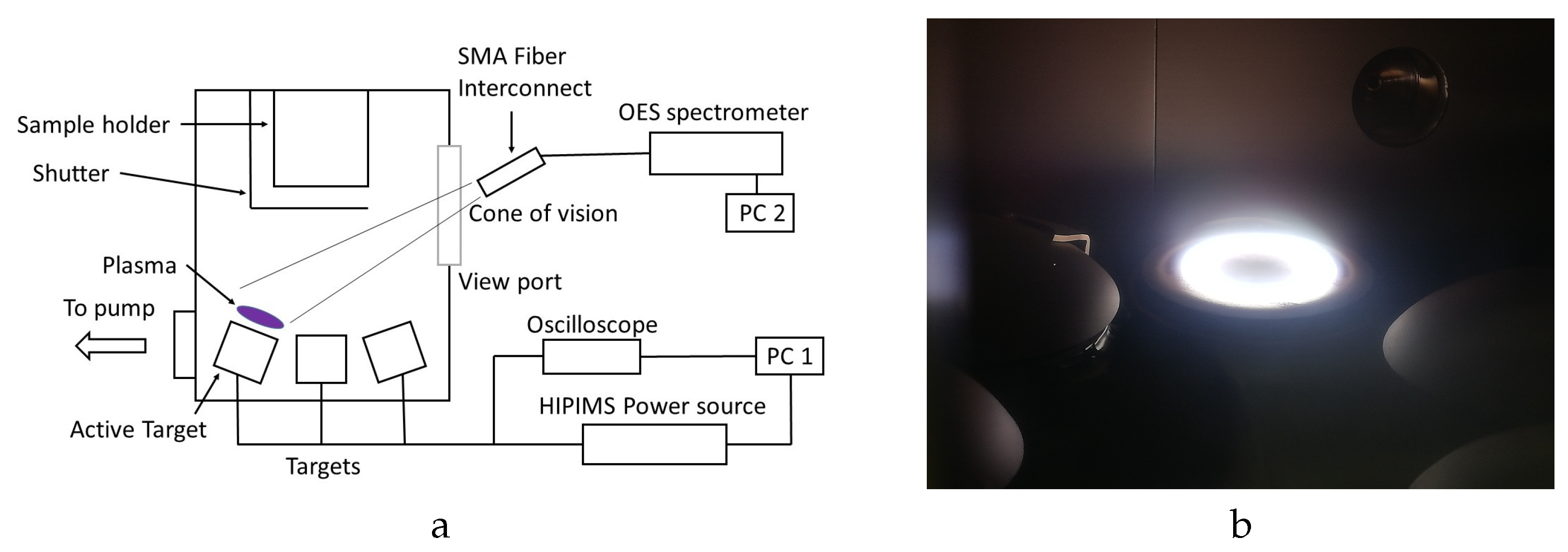
2. Materials and Methods

For the deposition, a Lesker PRO Line PVD 75 machine with a DC-power supply and a Starfire built pulse-unit, which regulates the HIPIMS-pulse and the kick-pulse, as well as a 3-inch gold target, were used. During the pulse, argon flow and pressure were regulated to 70 sccm and 5 mTorr, respectively. The employed measurement instruments are a digital oscilloscope, model Picoscope 2205A-D2, and a spectrometer, model Avantes ULS2048CL-EV, with a 25 µm slit that allows observations in the wavelength range between 200 nm and 1100 nm. For the OES measurements, an optical fibre with a diameter of 200 µm was directed from outside of the vacuum chamber towards the plasma, aimed down onto the racetrack under an oblique angle. The fibre was connected with the spectrometer and a SMA fibre interconnector, which allowed us to more easily direct the fibre and provided a narrow cone of vision, as the interconnector blocked the surrounding light. While light from the room illumination was also present in the spectrum, it was easily detectable, as the intensity was constant, and due to the nature of the illumination, only a few peaks stemmed from that light source. No collimator was used, as the light emanating from the plasma was deemed sufficiently bright for the measurements. Due to the lack of transparency of the viewport to UV-light, analysis of radiation at wavelengths shorter than 390 nm was not possible. The scheme of the used apparatus can be seen in Figure 1. The spectra were taken in a time-integrated mode with an integration time of 32 ms. Six targets were present in the machine. The targets were positioned in a circle with the targets tilted towards the sample holder. For experiments in this work, the gold target was on the furthermost position from the view port and was tilted towards the sample holder, while also being tilted towards the optical fibre. To avoid formation of metal films on the view port, a shutter was used, which is not included in Figure 1. This shutter was placed in front of the view port and opened for measurements. This allowed us to avoid distortion of the measured spectra.

The intensity depends on various factors, such as the concentration of a species, the plasma temperature, the electron density, the electron temperature, …expressed in equation $I=n_n{n}_{e}X(n_e,T_e\dots )$ [20], with $n_e$ being the electron density, $n_n$ being the density of the species and $X(\dots )$ being the effective emission rate coefficient depending on several factors.

For the estimation of the amount of gold in the plasma during a pulse, the line ratio was used. The ratio was simplified to:

$$\frac{I_1}{I_2}=k\frac{n_1}{n_2},$$

(3)

During the analysis, the following lines were used: Ar I (811 nm), Ar II (488 nm) and Au I (751 nm). For the identification of the peaks, the NIST spectral database was used [34]. These peaks are marked with straight arrows in Figure A1. The area of those peaks was integrated, while for all other mentioned peaks, only the peak height was used.

Due to the pulsed nature and variations within the pulse, time-resolved measurements, especially of electron density and temperature, would be useful for a further analysis. Additionally, an analysis of the resulting layers would be useful with regard to film density and thickness.

Other means of gold deposition are DC-PVD, RF-PVD and filtered arc deposition (FAD). The mentioned cases of DC-PVD [35] made use of low power input of 10 to 50 W [36,37] for the deposition of gold films with a thickness of 167.5 nm [36]. RF-PVD made use of similar power levels of 20 to 125 W [38,39]. Attempts to use arc deposition were also made [40] and compared to gold films deposited with thermal evaporation and magnetron sputtering. In similar conditions (ambient temperature, no substrate bias), the layers resulting from FAD were the smoothest. The use of HIPIMS for the deposition is quite new [41]. Usually, argon is the preferred gas for PVD-processes. The use of krypton and xenon for gold sputtering was reported in [42]. In [42], a quartz crystal microbalance was used for an analysis of the resulting films and the ionization.

3. Results

The results of variation in voltage, pulse length and the influence of the kick-pulse are described in this section. As an initial condition, a pulse length of 20 µs was chosen with a voltage of 1000 V and a frequency of 1 kHz, followed by a kick-pulse with an after-glow time of 5 µs, a voltage of 195 V and a width of 50 µs, in order to clearly demonstrate how the plasma is affected by the kick-pulse. Voltage and pulse lengths were varied for the measurements and the frequency was adapted for the longer pulse lengths. To analyse the effect of the kick-pulse, measurements were undertaken with the kick-pulse switched off and compared to a process in which the kick-pulse was utilized.

For further analyses of the plasma, the intensities of two argon-lines were considered and compared to evaluate the ionization. Due to its intensity, the Ar I line at 811 nm and the Ar II line at 488 nm were chosen, as both are clearly identifiable and both peaks are sufficiently separated from nearby peaks. The intensities of these lines differ by one order of magnitude. The scales in the diagrams were chosen in such a way that relative changes would be equally proportional.

Additionally the Au I line at 751 nm was chosen, as it has a similar size as the Ar I line. The choice of the mentioned Au I and Ar II lines also has an advantage in that the noise around those lines was sufficiently small, unlike that around the Ar II lines between 400 nm and 450 nm. Due to the absence of Au II peaks, no similar analysis could be carried out for gold.

The current curves were averaged from five measurements.

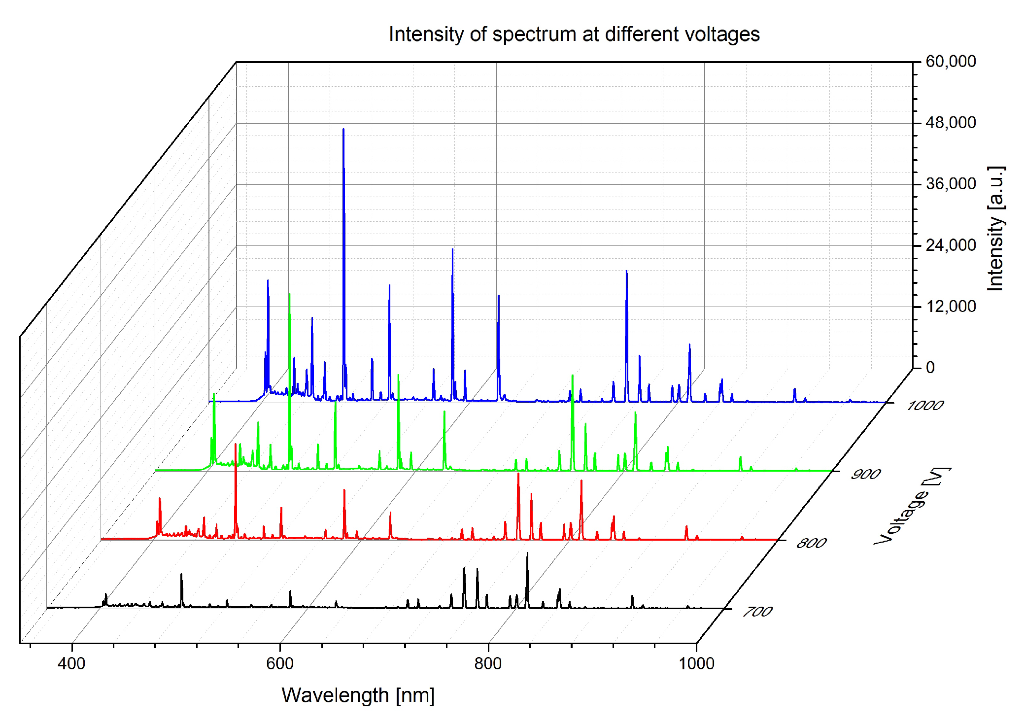
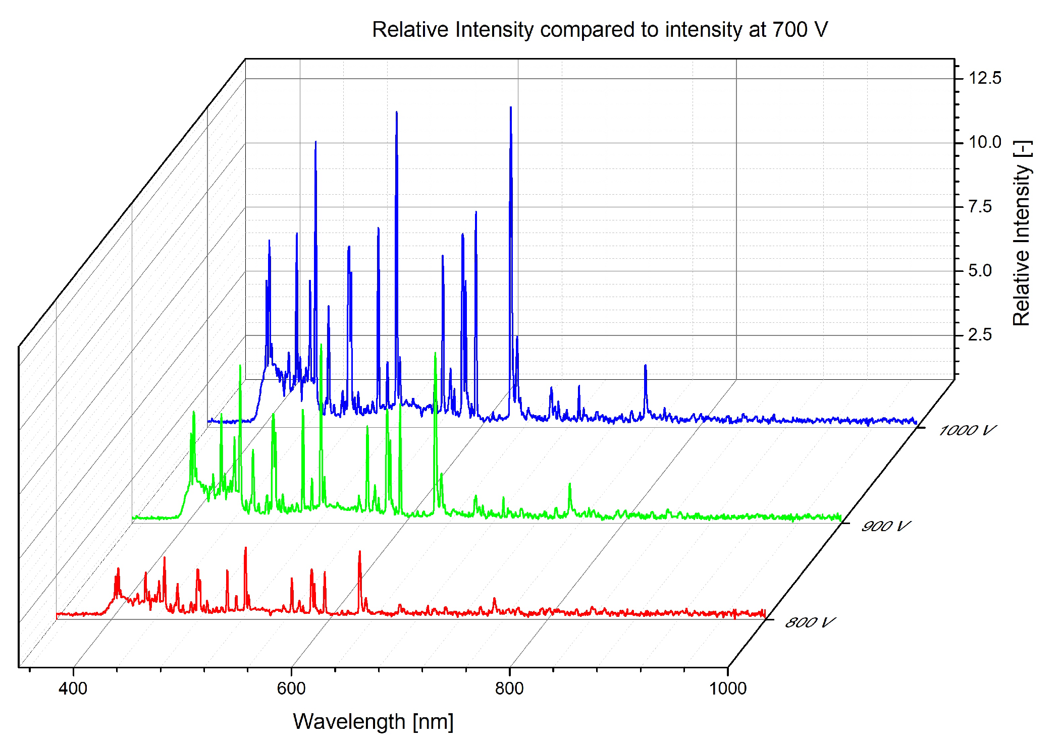
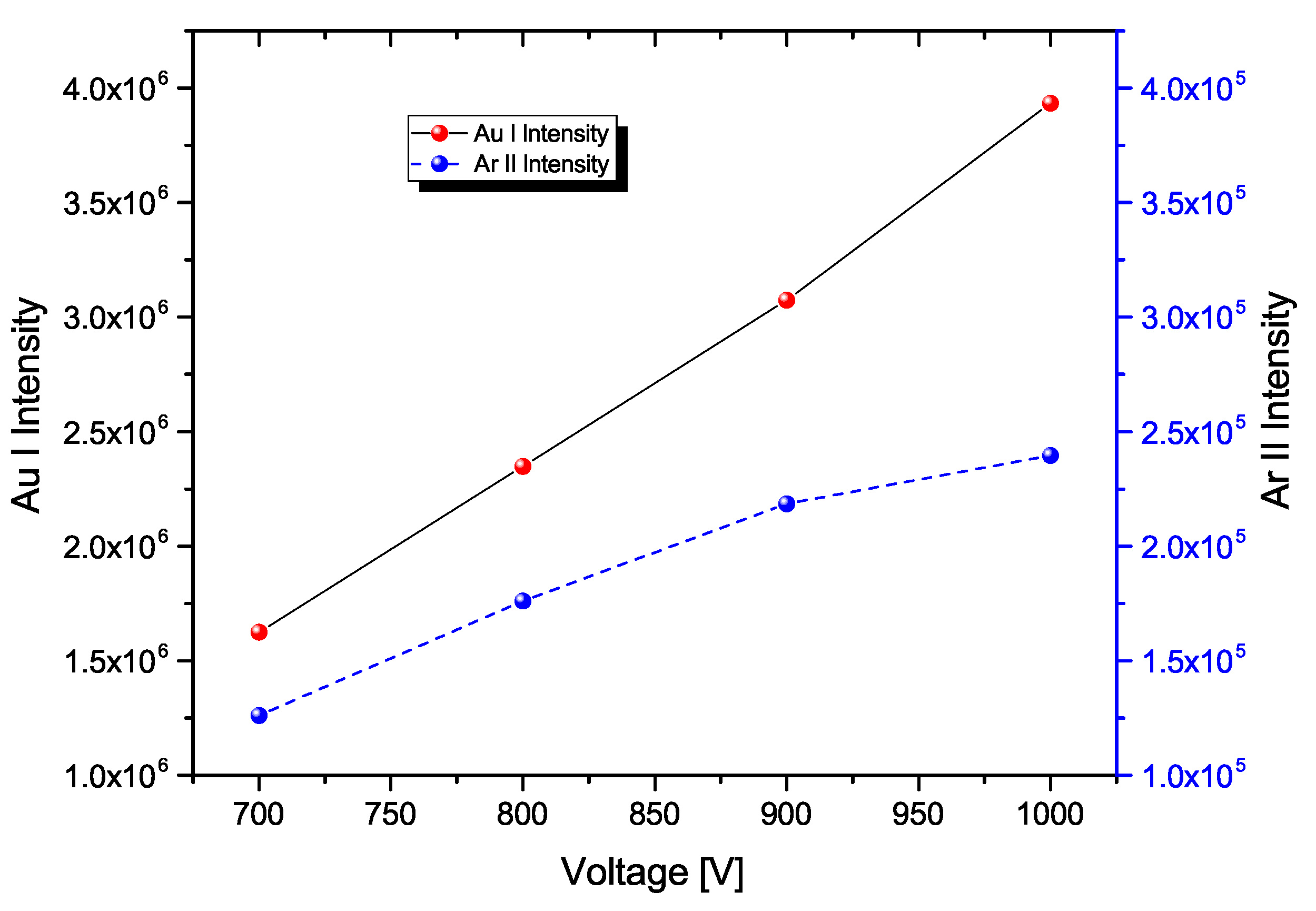
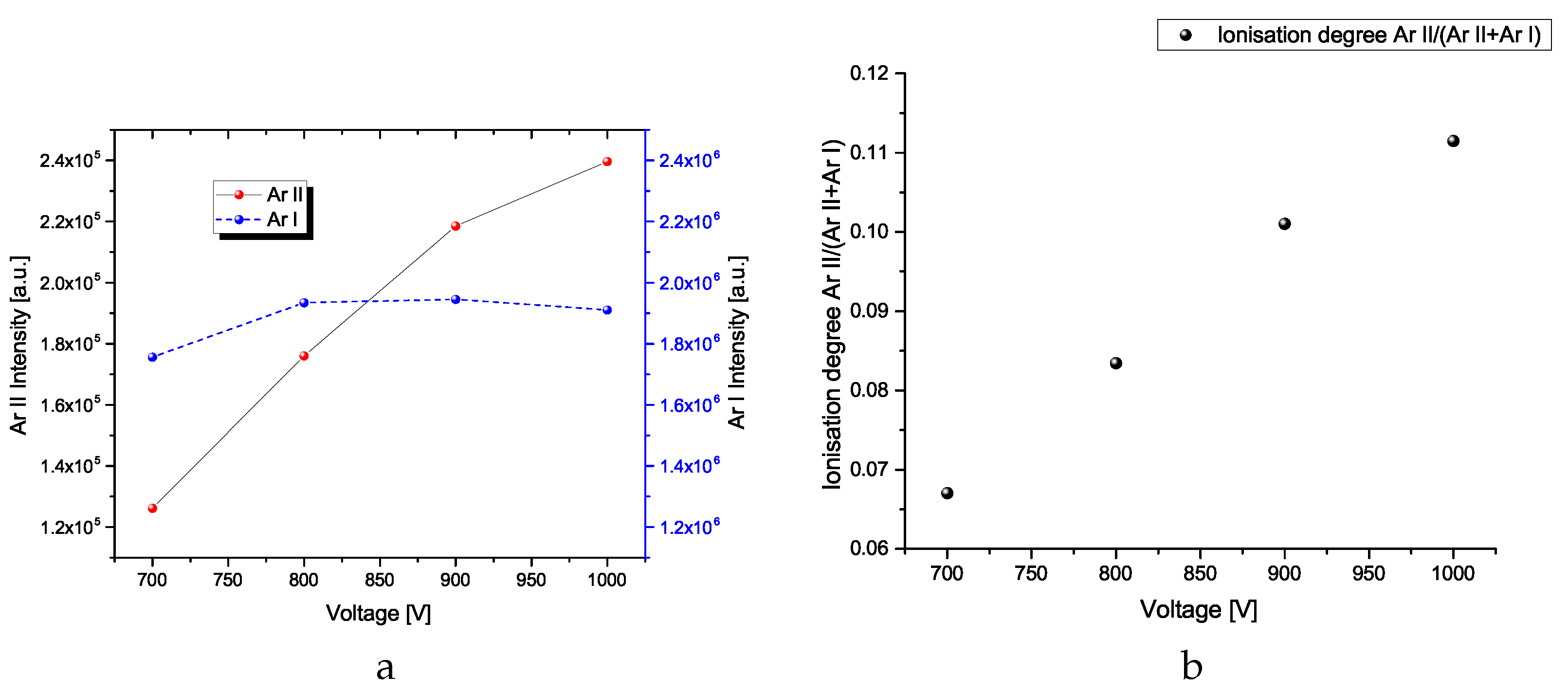
3.1. Influence of Voltage

The influence of voltage of the main pulse was analysed. The voltage was varied from 700 V to 1000 V using 100 V steps. The pulse-width was at 20 µs at a frequency of 1 kHz. The main pulse was followed by the kick-pulse with an after-glow time of 5 µs, a width of 50 µs and a voltage of 195 V.

As can be seen in Figure 2, the change in voltage leads to a considerable change in current.

The peak currents were measured shortly before the end of the 20 µs pulse. At 700 V, the peak current was equal to 121 mA/cm², rising to 179 mA/cm² at 800 V, 241 mA/cm² at 900 V and then growing to 317 mA/cm². Every 100 V increase from 700 V to 900 V led to a linear increase of approximately 60 mA/cm², and a final growth to 80 mA/cm² for the last step. While during the first 5 µs, the rising current was strongest for voltages over 800 V, for the rest of the pulse, the current increase was less pronounced. At 700 V, the current grew linearly with time. The peak current density was at the end of the pulse. Once the pulse ended, the current density decreased until the onset of the kick-pulse, which quenched the current below 0 mA/cm² for all cases.

The comparably slow increase in current indicates lower values of n in Equation (2) during the deposition of gold. The reason for that increase might be the rarefaction of plasma after the peak current was achieved or a decrease in electron trapping efficiency [11,12,15,43]. The reverse polarized kick-pulse accelerated the species away from the target, leading to an abrupt decrease in the current.

The spectrum of the process can be seen in Figure 3. At the shorter wavelengths below 650 nm, Au I peaks are clearly visible. The brightness of Au I outweighs the brightness of the Ar I peaks. While Ar I can be clearly seen at wavelengths above 650 nm, the peaks of the Ar II at shorter wavelengths are much smaller, and show growth with increasing voltage. No Au II peaks were found. If gold is ionized, the emissions are below the measurement sensitivity.

Contrary to the increase in current density, the changes in peak intensity are more pronounced, as can be seen in Figure 4. Here, the measurements at different voltages were compared to the initial measurement at 700 V, in order to see a change with increasing voltage. While Au I and Ar I are clearly very bright, the changes in voltage have a greater impact on the intensities of the Au I peaks, between the wavelengths of 400 nm and 650 nm. Equally, the intensities of the Ar II lines grow, albeit by a far smaller amount. Clearly, the brightness of the Au I changed, as can be seen in the up to 13-fold rise in the Au I peaks at 523 nm and 627 nm. Several other lines grow about eightfold. Contrary to the strong changes in Au I intensity, the peak height of Ar I does not change, as can be seen from the Ar I peaks between 700 nm and 800 nm, especially in case of the peak at 811 nm. While several Ar I peaks are present at wavelengths above 650 nm, the only peak that has a change in intensity in that wavelength range is the Au I peak at 751.45 nm. The changes in relative intensity are listed in

Table 1. Several Au I peaks can be seen in Figure 4. Relative changes in intensity between the respective voltages and the initial spectrum, measured at a voltage of 700 V, are listed.

Wavelength [nm]	800 V	900 V	1000 V
565.51	2.4	4.6	7.4
583.75	2.7	5.2	8.3
595.91	2.6	5.4	9.2
627.93	3.4	7.5	13.2

, with several lines roughly doubling every 100 V, thus having an exponential growth. A more exhaustive list can be found in

Table A1. Changes in Au I line intensities depending on voltage relative to a spectrum at 700 V.

Wavelength [nm]	800 V	900 V	1000 V
404	2.4	4.3	6.5
406	2.8	5.1	8.1
431	2.6	5.1	8.4
443	2.3	4.1	6.5
449	3.2	7	11.9
460	2.2	3.7	5.2
479	2.7	5.1	7.8
506	2.7	5.2	8.5
523	3.6	7.7	13.1
565	2.4	4.6	7.4
583	2.7	5.2	8.3
595	2.6	5.4	9.2
627	3.4	7.5	13.2
665	1.4	1.8	2.4
751	1.6	2.3	3.2

in Appendix A. The brightest Au I peaks stem from the transitions 7s → 6p (431 nm, 449 nm, 460 nm, 523 nm, 565 nm, 583 nm, 595 nm and 751 nm), 6p → 6s (404 nm, 506 nm and 627 nm) and 6d → 6p (406 nm and 479 nm).

Figure 5 shows the change in intensities of Au I and Ar II lines. As the voltage increases from 700 V to 900 V, both the Au I and the Ar II intensities increase linearly. A further voltage increase from 900 V to 1000 V leads to visible differences in the behaviour of the two lines. Contrary to the Ar II line, where the increase is less pronounced, the Au I lines increase even more. The Au I intensity follows the peak currents with changes in voltage.

The Figure 6 shows the intensities of both argon lines with rising voltage. While Ar I rises slightly from 700 V to 800 V and remains nearly unchanged, with a voltage increase up to 900 V, a slight decrease is visible once the voltage is at 1000 V. Contrary to Ar I, the Ar II intensity rises linearly from 700 V to 900 V, with a less pronounced increase towards 1000 V. The increase in ionization is linear from 700 V to 900 V, with a less pronounced increase from 900 V to 1000 V. The ionization degree is depicted in Figure 6.

An increase in Au I intensity becomes apparent as the voltage increases, while the Ar I intensity remains mostly constant. Starting from the increasing ratio of Au I to Ar I, we can assume an increase in the presence of gold in plasma, and thus an increase in the deposition rate. This result is supported by [42]. Whether an improvement in film quality can be expected is unclear, as here, an increase in ionization of the sputtered species is needed, but only an increase in argon ionization is observed.

A visual depiction of the plasma at initial conditions (1 kV, 1 kHz, 20 µs pulse length) can be seen in Figure 1. The change in brightness of the Au I lines translates into a change in the plasma colour from a faint violet glow at 700 V to a bright white glow at 1000 V. As the peaks are evenly spread out over the whole spectrum and have a mostly similar intensity, the plasma appears white.

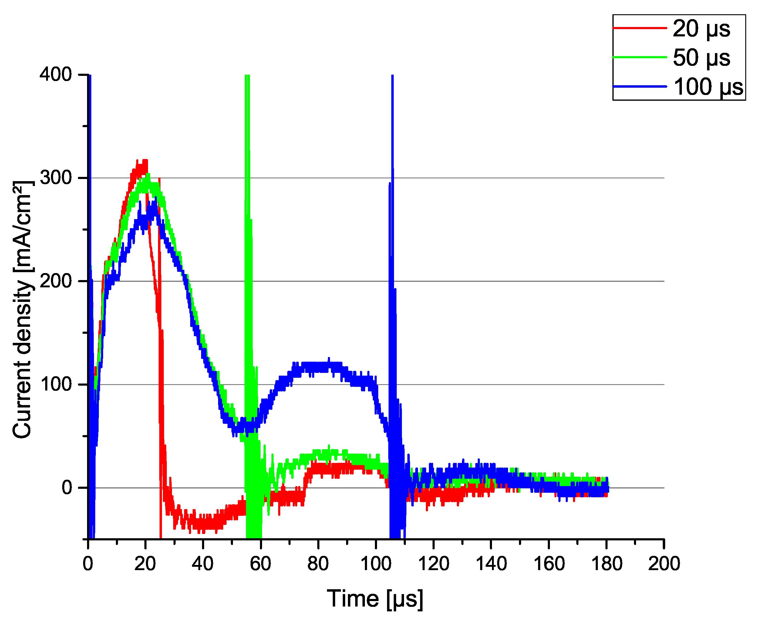
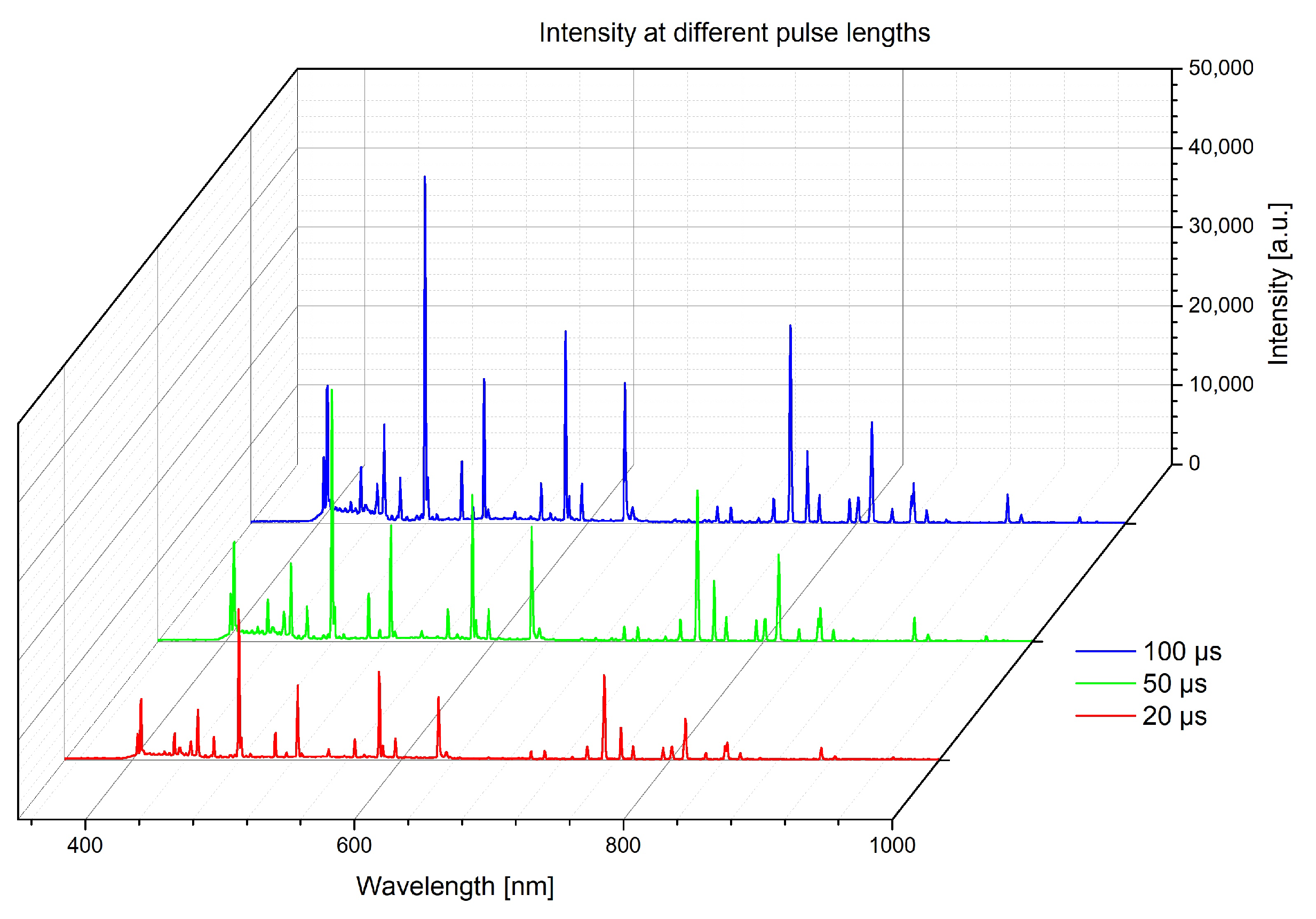
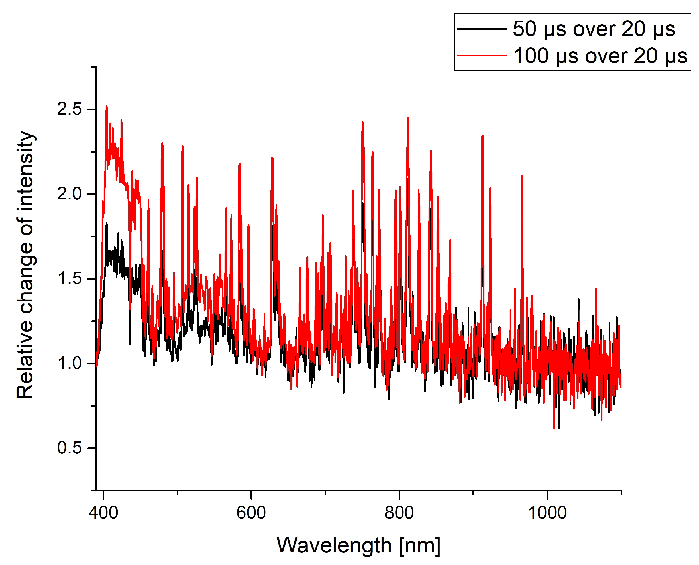
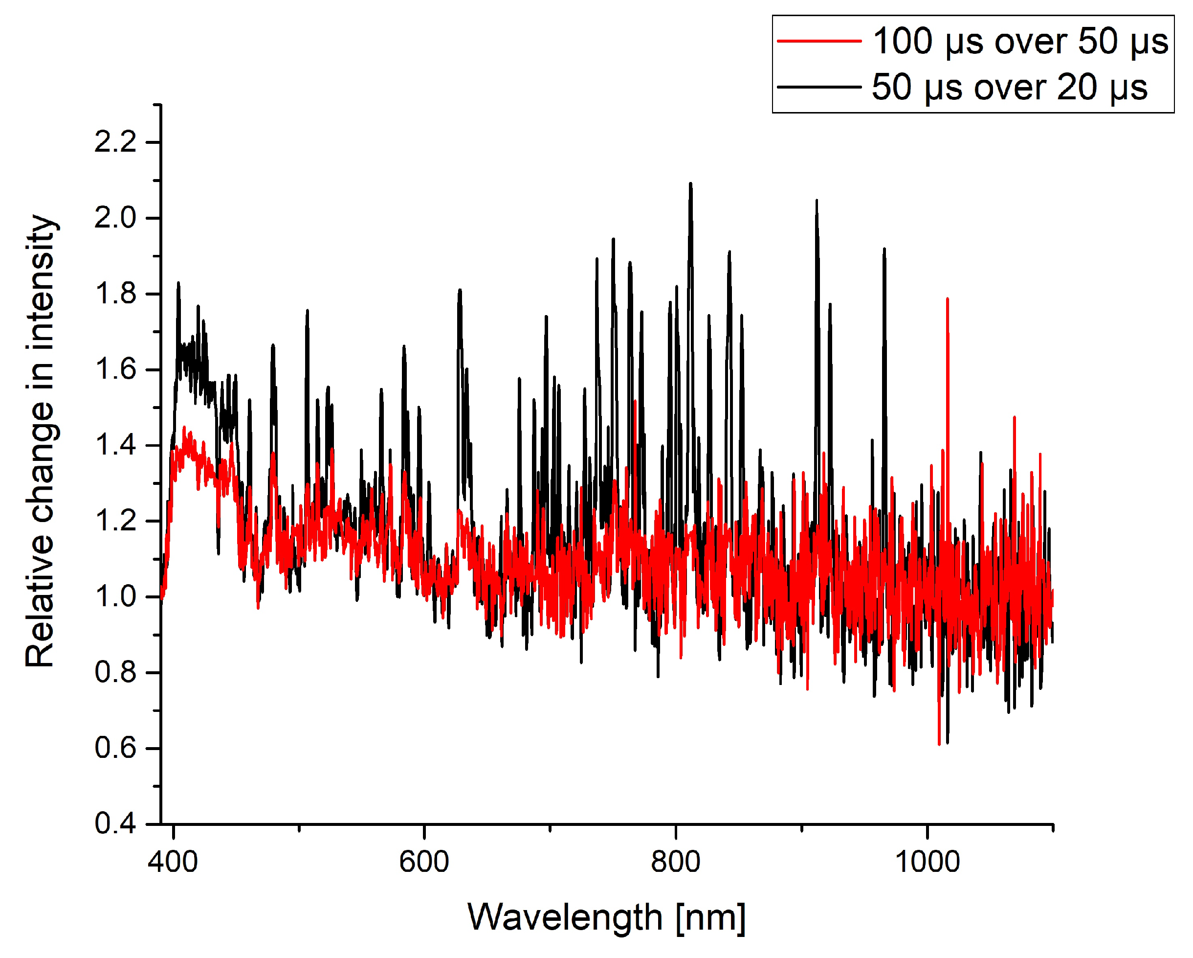
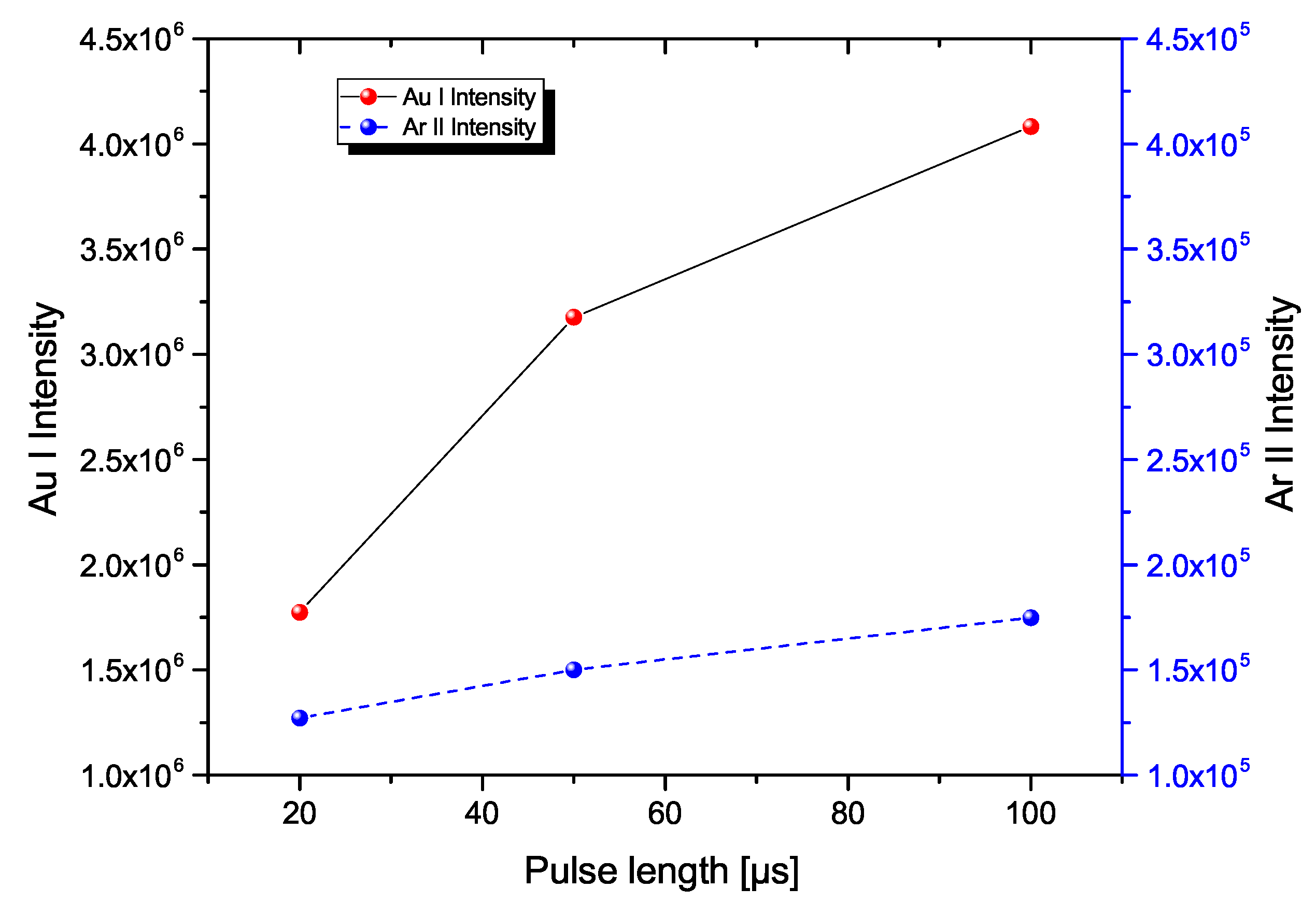
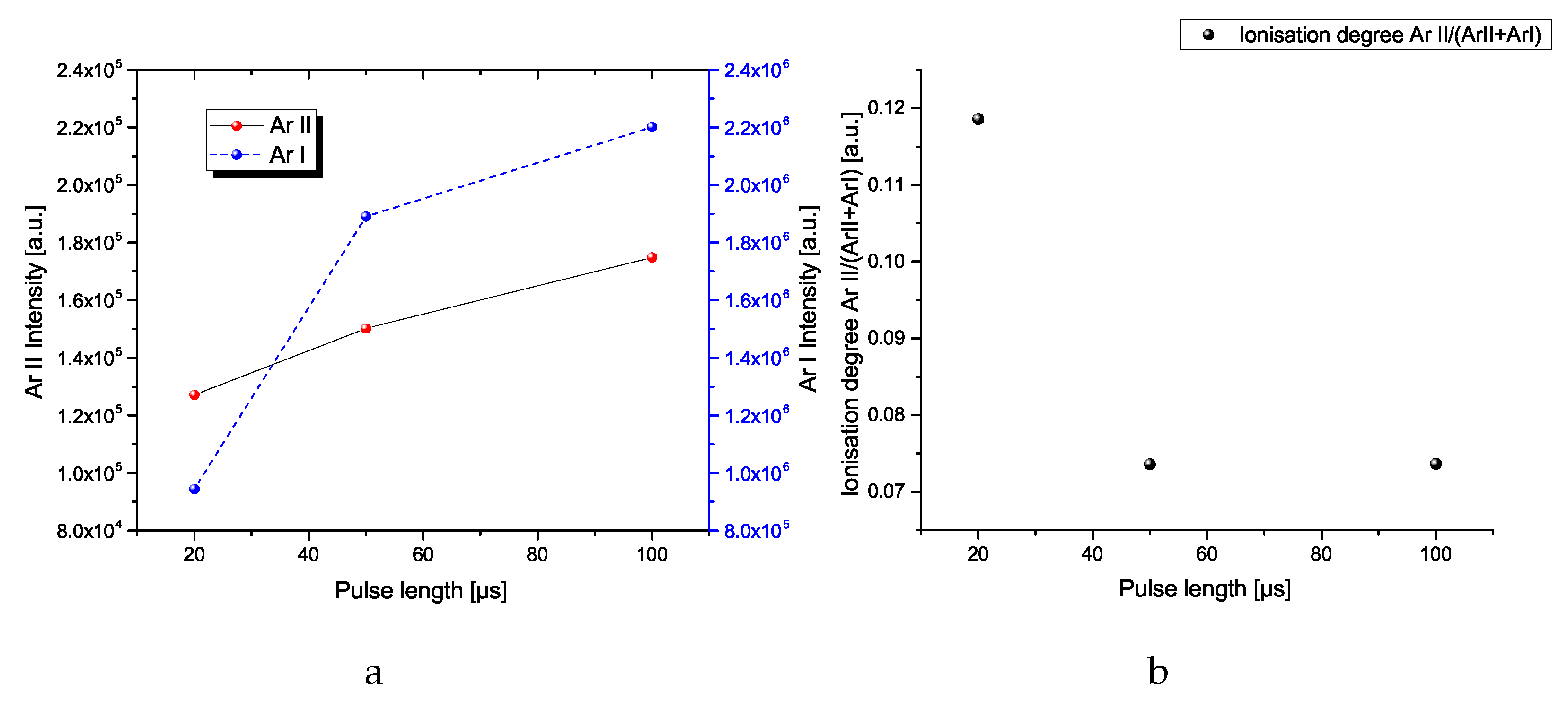
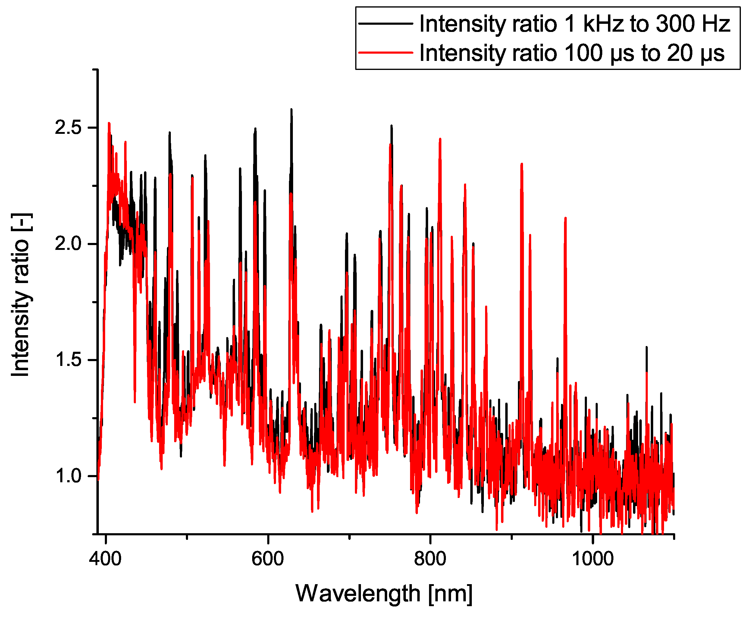
3.2. Influence of Pulse Length

For the analysis of the influence of different pulse lengths, three pulse lengths were chosen, namely 20 µs, 50 µs and 100 µs, followed by a reverse polarized pulse 5 µs after the end of the pulse, which had a voltage of 195 V and a length of 50 µs. The frequency was limited to 300 Hz for the spectroscopic measurements, as pulse lengths longer than 20 µs at a frequency of 1 kHz would result in power consumption above the limit of the power supply.

The current densities over time can be seen in Figure 7. For 20 µs and 50 µs, similar peak current densities of 300 mA/cm² are achieved, with slightly smaller values of around 275 mA/cm² for the 100 µs pulse. The shorter the pulse, the higher the peak current, which is at its highest for the 20 µs pulse with 317 mA/cm², 303mA/cm² for the 50 µs pulse and at its lowest at 281 mA/cm² for the 100 µs pulse. The peak current is achieved at 20 µs after the onset of the pulse. As for the 20 µs-pulse, the voltage falls to 0 mA/cm², and the current density also shrinks until the kick-pulse quenches any current below a current density of 0 mA/cm². After the peak, the 50 µs and the 100 µs-pulse decrease similarly to the same level, until the kick-pulse lowers the current density to 0 mA/cm². For the first 20 µs of the 100 µs pulse, similar current densities to the 50 µs pulse are achieved, peaking at about 300 mA/cm². The current density shrinks abruptly just afterwards, until it reaches a level of approximately 58 mA/cm². At about 55 µs after the peak onset, the current rises only slightly until it reaches approximately 121 mA/cm² at 77 µs, only to sink to 100 mA/cm² after 90 µs. It is then suppressed by the kick-pulse after the end of the main pulse. The reason for the waveform of the 100 µs-pulse is the rarefaction of argon after the main pulse, followed by a back-flow of argon after 60 µs, leading to a second rise and decrease in the current density.

Figure 8 shows the spectra of pulses with different pulse lengths.

The spectra for different pulse lengths increase in intensity with the increasing pulse length. The increase is not linear for Au I and Ar I, considering that the main contribution to the current occurs in the first 20 µs for all pulses and in the first 50 µs for the longer pulse lengths. Big differences for the spectra could not be expected, as the second peak of the 100 µs pulse reaches only a current density of up to 120 mA/cm², which, as described in Section 3.1, leads to peak intensities that are up to 13 times smaller compared to peaks occuring at a peak current density of 300 mA/cm². Despite the longer pulses, no Au II peak could be found. If ionization of Au II takes place, it cannot be identified, as the emission is below the measurement sensitivity. The reason for the lack of ionization may be due to the high ionization energy.

Figure 9 shows the relative difference in the spectra between the pulses. Two curves are depicted in this graph: one that shows the differences between a 50 µs pulse and a 20 µs pulse and a second one that depicts the differences between a 100 µs pulse and a 20 µs pulse. As could be expected, the brightness increases with the pulse length. The main difference concerns the Ar I peaks, which are more intense for the 100 µs pulses. Compared to the Ar I peaks, the Au I peaks are less pronounced compared to the background, indicating that while the pulse length doubled, the difference in intensity only increased by half. There is a roughly 1.6-fold increase in Au I line brightness between the 50 µs pulse and the 20 µs pulse. The 100 µs pulse leads to a 2.1-fold increase in Au I intensity compared to the initial pulse. Hence, gold is sputtered mainly in the first 10 µs of the pulse and the length of the pulse does not translate linearly into the presence of gold in the plasma. An up to twofold increase in brightness between the 50 µs pulse and the 20 µs pulse could be expected, because the longer pulse is not interrupted by the end of the voltage pulse and the kick-pulse.

In Figure 10 the relative changes in intensities between the 50 µs pulse and the 20 µs pulse are compared to the changes between the 100 µs pulse and the 50 µs pulse. With increasing pulse length, the peak height does not grow linearly. While more than doubling the pulse length from 20 µs to 50 µs leads to an about two-fold increase in peak height over the whole spectrum, the effect is not as pronounced when increasing the pulse length from 50 µs to 100 µs. For the changes from 50 µs to 100 µs, the peak intensity increases by 20% to 40%. The difference in brightness of the gold-peaks does not stand out as much from the background. A fivefold increase in pulse length does not lead to a fivefold increase of brightness. The Au I peaks do not stand out from the spectrum. This result was expected, as the second peak of the 100 µs pulse is smaller than the main peak and reaches only one-third of the current density of the main peak, which, as seen in Section 3.1 translates to an up to 13-fold difference in the peak height of several Au I peaks.

Figure 11 shows the changes in intensities of Au I and Ar II lines. Both the Au I and the Ar II lines increase in intensity. While the Ar II intensity increases linearly with increasing pulse length, the Au I intensity nearly doubles from 20 µs to 50 µs. The growth is far less pronounced for the doubled pulse length, which increases from 50 µs to 100 µs. The behaviour of the Au I line coincides with the discharge current, where the main part occurs in the first 50 µs and the second part is far less pronounced. Still, the Au I to Ar II ratio increases with the pulse length. The Au I line coincides well with the discharge current, where the main contribution to the current occurs in the first 50 µs.

Figure 12 show the evolution of Ar I and Ar II intensities for increasing pulse lengths (a) and the changes in ionization degree (b). It can clearly be seen that the intensities of Ar I and Ar II are an order of magnitude apart, with the Ar I emission being more intense. For both species, an increase in brightness can be observed, albeit with differences. While the Ar I line roughly doubles for the increase in pulse length from 20 µs to 50 µs, the increase for the doubled pulse length from 50 µs to 100 µs is only minimal, with about a tenth of additional intensity. This change follows the discharge currents in Figure 7, where the main contribution to the current is within the first 50 µs and only a minor contribution occurs for the last 50 µs. Contrary to that observation, the Ar II intensity increases in a nearly linear fashion. The nearly linear increase is similar to the evolution of the Au I intensity. The strong increase in Ar I intensity for the short pulses leads to a decrease in ionization of the argon for an increase in pulse length from 20 µs to 50 µs and a remaining low ionization degree for an increase in pulse length from 50 µs to 100 µs. Despite the pronounced rarefaction, the Ar II intensity grows with longer pulse lengths.

In general, shorter pulses are advised for a more efficient deposition [44]. With a pronounced rarefaction, the presence of gold in the plasma is reduced as can be seen based on the minor increase in Au I intensity compared to the pulse length. As such, we can expect a relative decrease in the deposition rate with regard to the on-time of the target. As no ionization is observed, which would be necessary for self-sputtering, we can assume that its contribution to the sputtering process is of minor—if any—importance.

Figure 13 offers a comparison between an increase in frequency compared to an increase in pulse length. In one case, the active time more than tripled, while in the other case, it rose fivefold. Here, red shows the relative change for increasing pulse length from 20 µs to 100 µs and black for the increase in frequency from 300 Hz to 1 kHz. Overall, we see a less efficient process with longer pulses. Despite being active over a shorter timespan, the intensity of the Au I lines is higher and the ratio of Au I lines compared to Ar I lines is visibly higher for the increased frequency. While the target is active for a shorter time, the Au I intensity and the Au I to Ar I intensity is higher. Still, increasing frequency does not translate to a linear increase in intensity.

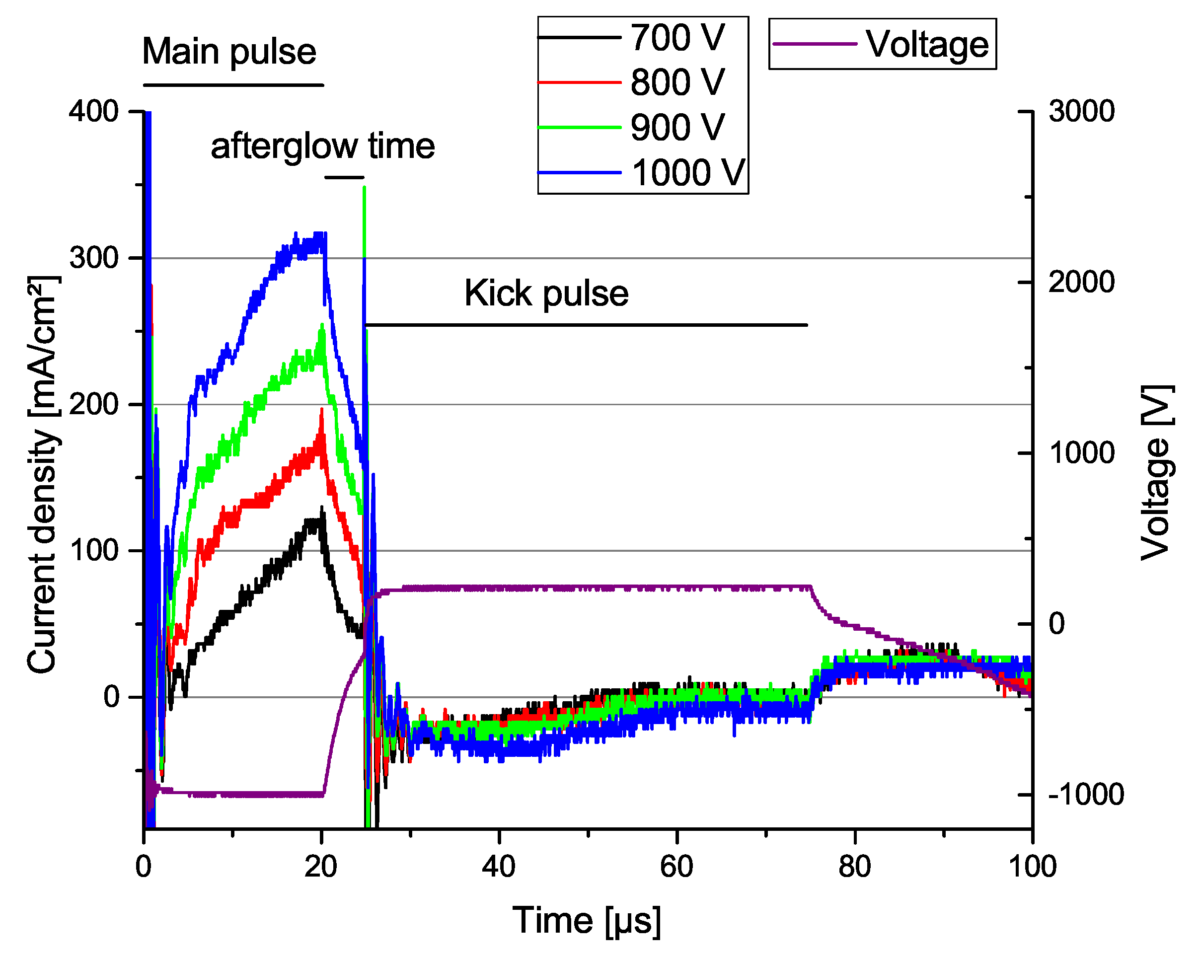
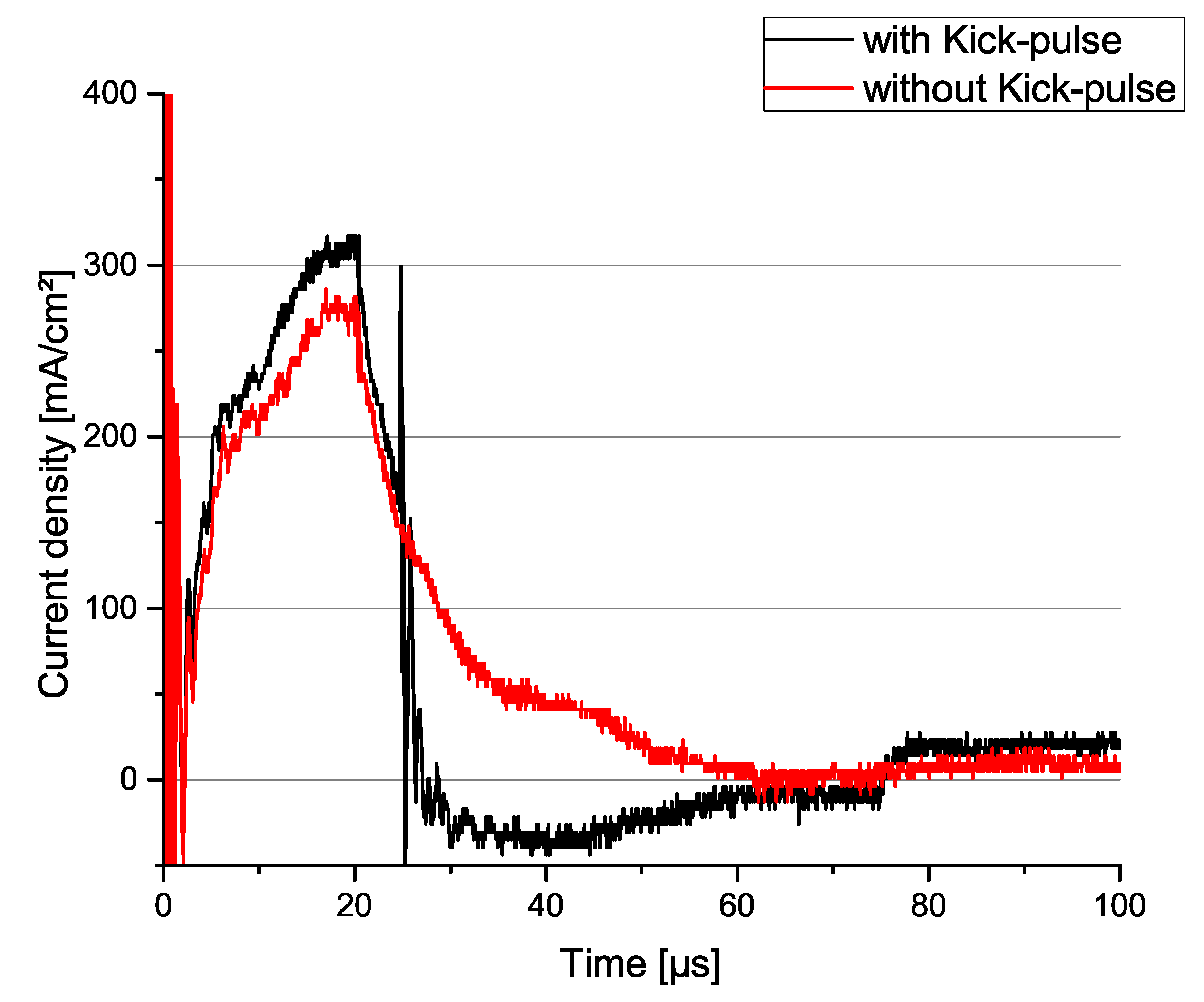
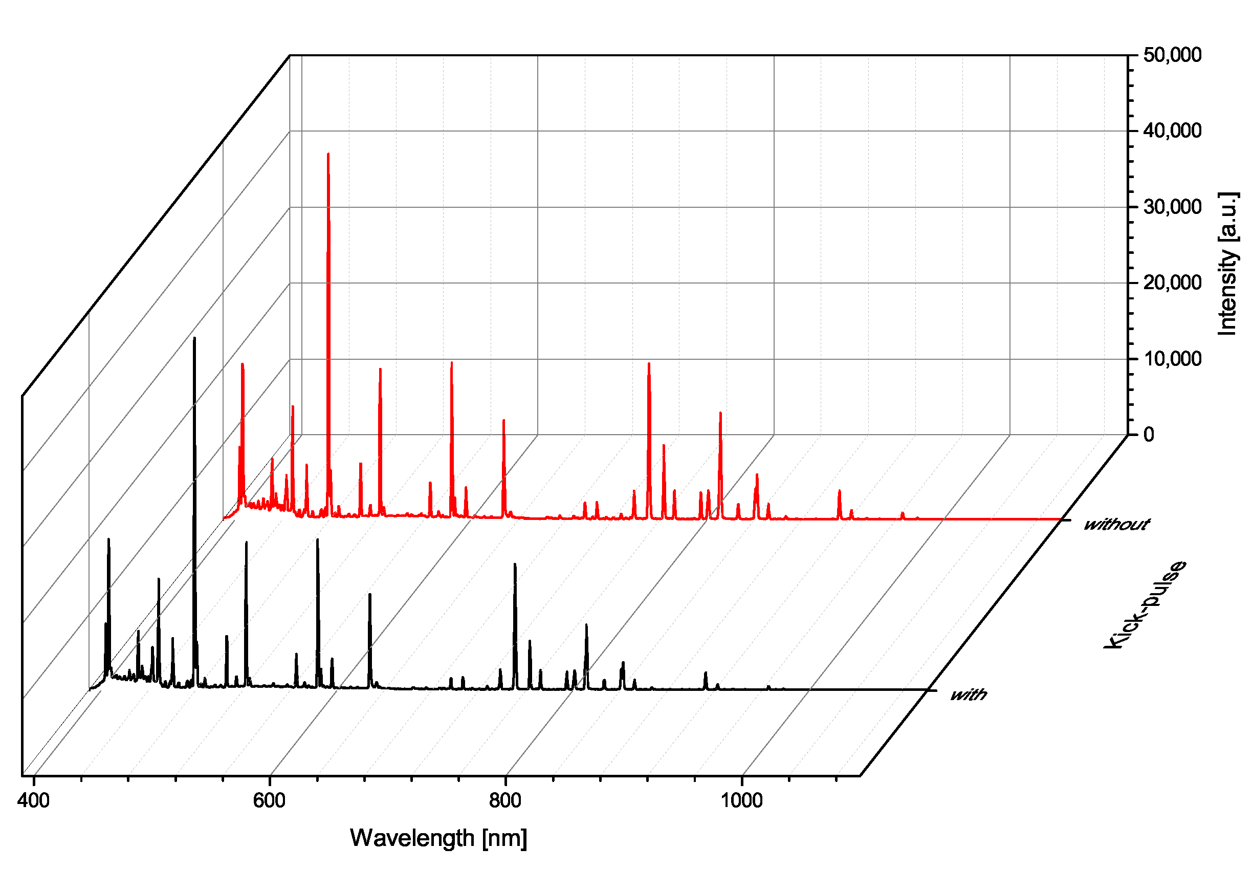
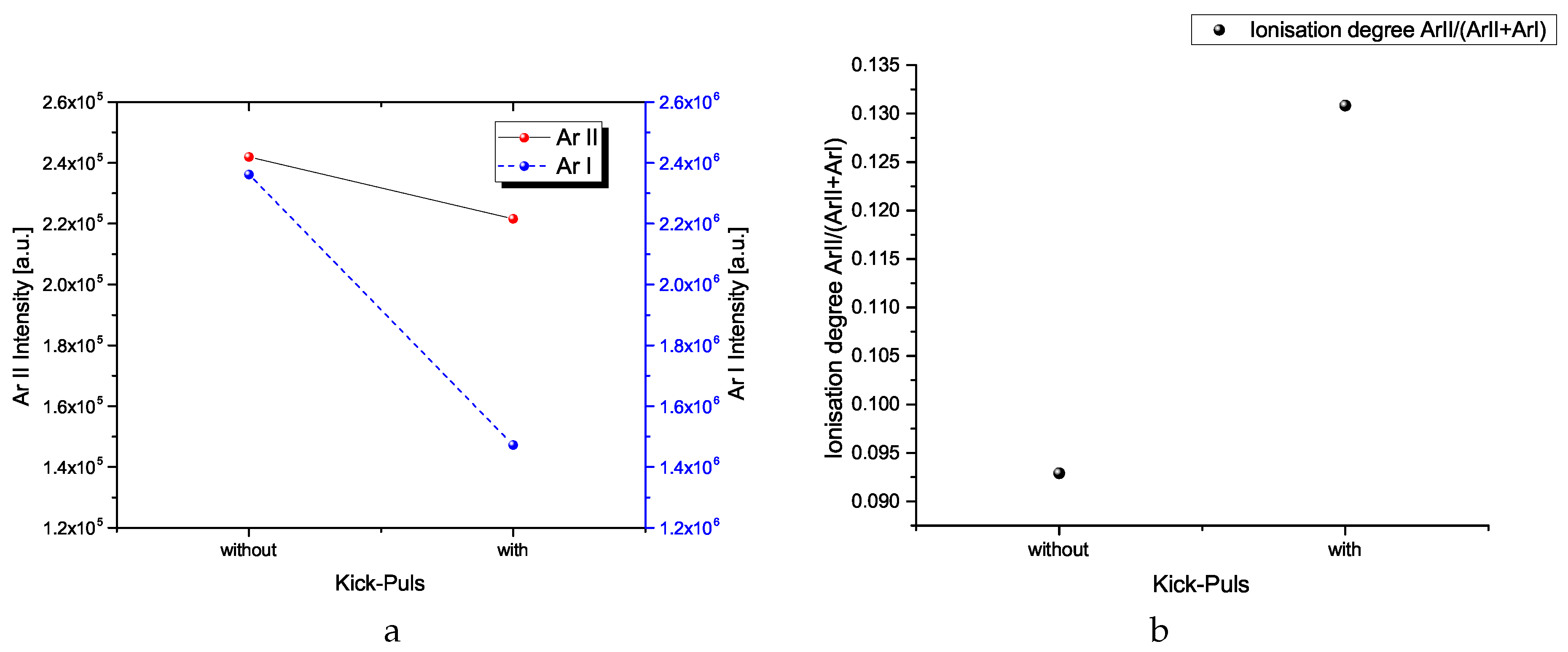
3.3. Influence of Kick-Pulse

For these measurements, a main pulse with a length of 20 µs and a voltage of 1 kV was chosen. The kick-pulse followed only 5 µs after the main pulse, with a voltage of 195 V and a width of 50 µs.

Figure 14 shows the currents during pulses with and without the kick-pulse. For the main pulse, the curves are similar until the onset of the kick-pulse, 5 µs after the end of the main pulse. Once the kick-pulse has been applied, the current is quenched below 0 mA/cm². If no kick-pulse is applied, the current density sinks below 0 mA/cm² after 60 µs and arrives at 0 mA/cm² after 80 µs. After 60 µs, the current densities are equal. A difference in the peak current is visible. While the peak current of the pulse with kick-pulse is 317 mA/cm², the pulse without kick-pulse has a peak current of only 277 mA/cm².

Figure 15 shows the different spectra during pulses with and without a kick-pulse. As shown, Ar I shows the biggest difference, being visibly brighter when the kick-pulse is absent, compared to a process with a kick-pulse. The loss of current density after the onset of the kick-pulse translates directly into a decrease in the brightness of plasma, and hence the intensity of the Ar I spectral lines. Contrary to Ar I, Ar II and Au I show no differences.

Figure 16 shows the relative changes between two spectra. The spectrum below and above 650 nm wavelength is affected in different amounts. The part with shorter wavelengths is between 400 nm and 650 nm and the longer wavelengths are between 650 nm and 1000 nm. In the wavelength range between 400 nm and 650 nm, no Au I peak stands out from the background. Only Ar I and, to a minor extent, Ar II peaks are visible.

At the same time, the impact on the Ar I is more pronounced, as is visible in the wavelength range between 650 nm and 1000 nm. For most lines, there is an an approximately 1.6-fold increase in intensity. As expected, the intensity of the plasma emissions decreases due to atoms being accelerated away from the target, which is clearly seen in the decrease in the Ar I line intensities. At the same time, virtually no change in Au I brightness could be observed, indicating an absence of gold in the plasma after the end of the main pulse, assuming that excitation of gold atoms would occur, if they were present in a sufficient amount.

Figure 17a,b show the change in intensities and the ionization degree. The difference in intensities for Ar I and Ar II is clearly visible with a more distinct relative change in intensity for the Ar I and a minor change for the Ar II peak. The reason probably stems from the difference in the presence of excited argon in the plasma after the end of the main pulse compared to ionized argon. That difference leads to changes in the ionization degree of argon, with ionization being higher for the process with kick-pulse.

The apparently smaller ionization degree from the process in which no kick-pulse was applied might be due to the presence of excited argon after the end of the main pulse. The influence of the kick-pulse is non-negligible, as the difference in the ionization degree was 41% higher for the process in which the kick-pulse was employed compared to the process where it was not.

4. Conclusions

The deposition of gold via HIPIMS is interesting, as it allows us to directly metallize polyimide. In order to provide information for future use, the influence of several parameters was analysed. Higher voltages led to a strong increase in excited gold atom presence in plasma, as can be seen in the spectra.

At the same time, an increase in voltage led to a minor increase in Ar I intensity from 700 V to 800 V and a small decrease when the voltage increased from 900 V to 1000 V. Contrary to Ar I, the intensity of Ar II increased in a mostly linear fashion with rising voltage, resulting in a linear increase in ionization.

The peak current grew linearly with increasing voltage. Analysis of the influence of various pulse lengths led to the observation that during the HIPIMS deposition of gold, a very pronounced rarefaction took place, limiting the usefulness of pulses longer than 20 µs. The presence of excited gold and argon atoms followed the evolution of the discharge current. The ionization of argon continued linearly with time, as evidenced by the increase in Ar II intensity. Longer pulses did not lead to measurable ionization of gold.

In order to achieve the step from a low-density discharge to a high-density discharge, whereby the ionization of gold and self-sputtering can be expected, a voltage above 1000 V would be necessary. The strong increase in Au I lines, while Ar I lines show only minor changes during an increase in voltage, can be exploited to control the deposition via OES, whereby the power or voltage of a process is controlled via the line-ratios of the present species of the spectrum.

The differences in a spectrum between a process with and without a kick-pulse were described. The presence of excited argon in the afterglow was strongly affected by the use of the kick-pulse. The emissions from excited gold atoms were below the measurement sensitivity and could not be identified. Ionized argon appeared to be less affected than excited argon.

Short pulses and high voltages were beneficial for the deposition, as higher voltages led to a strong increase in the amount of excited gold atoms, and short pulses appeared to be more efficient; thus, higher deposition rates could be expected.

For an evaluation of the layer quality, deposition with following analysis of the resulting would be necessary.

In future work, the relation between the intensity of gold and the resulting gold layers could be analysed, as well as the influence of the kick-pulse.

References

1. Adamovich, I.; Agarwal, S.; Ahedo, E.; Alves, L.L.; Baalrud, S.; Babaeva, N.; Bogaerts, A.; Bourdon, A.; Bruggeman, P.; Canal, C.; et al. The 2022 Plasma Roadmap: Low temperature plasma science and technology. J. Phys. Appl. Phys. 2022, 55, 373001. [Google Scholar] [CrossRef]
2. Mumtaz, S.; Khan, R.; Rana, J.N.; Javed, R.; Iqbal, M.; Choi, E.H.; Han, I. Review on the Biomedical and Environmental Applications of Nonthermal Plasma. Catalysts 2023, 13, 685. [Google Scholar] [CrossRef]
3. Kouznetsov, V.; Macak, K.; Schneider, J.M.; Helmersson, U.; Petrov, I. A novel pulsed magnetron sputter technique utilizing very high target power densities. Surf. Coat. Technol. 1999, 122, 290–293. [Google Scholar] [CrossRef]
4. Mozgrin, D.V.; Fetisov, I.; Khodachenko, G. High-current low-pressure quasi-stationary discharge in a magnetic field: Experimental research. Plasma Phys. Rep. 1995, 21, 400–409. [Google Scholar]
5. Benzeggouta, D. Etude de Procédés de Dépôts de Films Minces par Décharge Magnétron Fortement Ionisée. Ph.D. Thesis, Université Paris-Sud, Paris, France, 2008. [Google Scholar]
6. Helmersson, U.; Lattemann, M.; Bohlmark, J.; Ehiasarian, A.P.; Gudmundsson, J.T. Ionized physical vapor deposition (IPVD): A review of technology and applications. Thin Solid Film. 2006, 513, 1–24. [Google Scholar] [CrossRef]
7. Power, R.; Rossnagel, S. PVD for Microelectronics: Sputter Deposition Applied to Semiconductor Manufacturing; Academic Press: Cambridge, MA, USA, 1999; Volume 26. [Google Scholar]
8. Ehiasarian, A.P. High-power impulse magnetron sputtering and its applications. Pure Appl. Chem. 2010, 82, 1247–1258. [Google Scholar] [CrossRef]
9. Tiron, V.; Velicu, I.L.; Matei, T.; Cristea, D.; Cunha, L.; Stoian, G. Ultra-short pulse HiPIMS: A strategy to suppress arcing during reactive deposition of SiO2 thin films with enhanced mechanical and optical properties. Coatings 2020, 10, 633. [Google Scholar] [CrossRef]
10. Anders, A. Discharge physics of high power impulse magnetron sputtering. Surf. Coat. Technol. 2011, 205, S1–S9. [Google Scholar] [CrossRef]
11. Papa, F.; Gerdes, H.; Bandorf, R.; Ehiasarian, A.; Kolev, I.; Braeuer, G.; Tietema, R.; Krug, T. Deposition rate characteristics for steady state high power impulse magnetron sputtering (HIPIMS) discharges generated with a modulated pulsed power (MPP) generator. Thin Solid Film. 2011, 520, 1559–1563. [Google Scholar] [CrossRef]
12. Gudmundsson, J.; Brenning, N.; Lundin, D.; Helmersson, U. High power impulse magnetron sputtering discharge. J. Vac. Sci. Technol. Vac. Surfaces Film. 2012, 30, 030801. [Google Scholar] [CrossRef]
13. Anders, A.; Čapek, J.; Hála, M.; Martinu, L. The ‘recycling trap’: A generalized explanation of discharge runaway in high-power impulse magnetron sputtering. J. Phys. Appl. Phys. 2011, 45, 012003. [Google Scholar] [CrossRef]
14. Čapek, J.; Hála, M.; Zabeida, O.; Klemberg-Sapieha, J.; Martinu, L. Steady state discharge optimization in high-power impulse magnetron sputtering through the control of the magnetic field. J. Appl. Phys. 2012, 111, 023301. [Google Scholar] [CrossRef]
15. Rossnagel, S.M.; Kaufman, H. Current–voltage relations in magnetrons. J. Vac. Sci. Technol. Vac. Surf. Film. 1988, 6, 223–229. [Google Scholar] [CrossRef]
16. Zuo, X.; Zhang, D.; Chen, R.; Ke, P.; Odén, M.; Wang, A. Spectroscopic investigation on the near-substrate plasma characteristics of chromium HiPIMS in low density discharge mode. Plasma Sources Sci. Technol. 2020, 29, 015013. [Google Scholar] [CrossRef]
17. Vetushka, A.; Ehiasarian, A.P. Plasma dynamic in chromium and titanium HIPIMS discharges. J. Phys. Appl. Phys. 2007, 41, 015204. [Google Scholar] [CrossRef]
18. Olejnícek, J.; HubiČka, Z.; Kohout, M.; Kšírová, P.; Brunclíková, M.; Kment, Š.; Čada, M.; Darveau, S.A.; Exstrom, C.L. Optical emission spectroscopy of high power impulse magnetron sputtering (HiPIMS) of CIGS thin films. In Proceedings of the 2014 IEEE 40th Photovoltaic Specialist Conference (PVSC), Denver, CO, USA, 8–13 June 2014; pp. 1666–1669. [Google Scholar]
19. Karzin, V.; Karapets, K. Investigation of gas discharge features during HiPIMS using optical emission spectroscopy. Iop Conf. Ser. Mater. Sci. Eng. 2018, 387, 012029. [Google Scholar] [CrossRef]
20. Fantz, U. Basics of plasma spectroscopy. Plasma Sources Sci. Technol. 2006, 15, S137. [Google Scholar] [CrossRef]
21. Wu, B.; Haehnlein, I.; Shchelkanov, I.; McLain, J.; Patel, D.; Uhlig, J.; Jurczyk, B.; Leng, Y.; Ruzic, D.N. Cu films prepared by bipolar pulsed high power impulse magnetron sputtering. Vacuum 2018, 150, 216–221. [Google Scholar] [CrossRef]
22. Fernández-Martínez, I.; Santiago, J.A.; Mendez, Á.; Panizo-Laiz, M.; Diaz-Rodríguez, P.; Mendizábal, L.; Díez-Sierra, J.; Zubizarreta, C.; Monclus, M.A.; Molina-Aldareguia, J. Selective Metal Ion Irradiation Using Bipolar HIPIMS: A New Route to Tailor Film Nanostructure and the Resulting Mechanical Properties. Coatings 2022, 12, 191. [Google Scholar] [CrossRef]
23. Batková, Š.; Čapek, J.; Rezek, J.; Čerstvỳ, R.; Zeman, P. Effect of positive pulse voltage in bipolar reactive HiPIMS on crystal structure, microstructure and mechanical properties of CrN films. Surf. Coat. Technol. 2020, 393, 125773. [Google Scholar] [CrossRef]
24. Bai, X.; Cai, Q.; Xie, W.; Zeng, Y.; Zhang, X. Effect of ion control strategies on the deposition rate and properties of copper films in bipolar pulse high power impulse magnetron sputtering. J. Mater. Sci. 2022, 58, 1243–1259. [Google Scholar] [CrossRef]
25. Viloan, R.P.B.; Helmersson, U.; Lundin, D. Copper thin films deposited using different ion acceleration strategies in HiPIMS. Surf. Coat. Technol. 2021, 422, 127487. [Google Scholar] [CrossRef]
26. Avino, F.; Fonnesu, D.; Koettig, T.; Bonura, M.; Senatore, C.; Fontenla, A.P.; Sublet, A.; Taborelli, M. Improved film density for coatings at grazing angle of incidence in high power impulse magnetron sputtering with positive pulse. Thin Solid Film. 2020, 706, 138058. [Google Scholar] [CrossRef]
27. Huber, W.; Houlahan, T.; Jeckell, Z.; Barlaz, D.; Haehnlein, I.; Jurczyk, B.; Ruzic, D.N. Time-resolved electron energy distribution functions at the substrate during a HiPIMS discharge with cathode voltage reversal. Plasma Sources Sci. Technol. 2022, 31, 065001. [Google Scholar] [CrossRef]
28. Zanáška, M.; Lundin, D.; Brenning, N.; Du, H.; Dvořák, P.; Vašina, P.; Helmersson, U. Dynamics of bipolar HiPIMS discharges by plasma potential probe measurements. Plasma Sources Sci. Technol. 2022, 31, 025007. [Google Scholar] [CrossRef]
29. Michiels, M.; Godfroid, T.; Snyders, R.; Britun, N. A poly-diagnostic study of bipolar high-power magnetron sputtering: Role of electrical parameters. J. Phys. Appl. Phys. 2020, 53, 435205. [Google Scholar] [CrossRef]
30. Law, M.A.; Estrin, F.L.; Bowden, M.D.; Bradley, J.W. Diagnosing asymmetric bipolar HiPIMS discharges using laser Thomson scattering. Plasma Sources Sci. Technol. 2021, 30, 105019. [Google Scholar] [CrossRef]
31. Hippler, R.; Cada, M.; Hubicka, Z. Time-resolved diagnostics of a bipolar HiPIMS discharge. J. Appl. Phys. 2020, 127, 203303. [Google Scholar] [CrossRef]
32. Hippler, R.; Cada, M.; Stranak, V.; Hubicka, Z. Time-resolved optical emission spectroscopy of a unipolar and a bipolar pulsed magnetron sputtering discharge in an argon/oxygen gas mixture with a cobalt target. Plasma Sources Sci. Technol. 2019, 28, 115020. [Google Scholar] [CrossRef]
33. Guljakow, J.; Lang, W. Adhesion of HIPIMS-Deposited Gold to a Polyimide Substrate. Coatings 2023, 13, 250. [Google Scholar] [CrossRef]
34. NIST Atomic Spectra Database. Available online: https://physics.nist.gov/PhysRefData/ASD/lines_form.html (accessed on 7 November 2023).
35. Yahya, K. Effect of electrode separation in magnetron DC plasma sputtering on grain size of gold coated samples. Iraqi J. Phys. 2017, 15, 202–210. [Google Scholar] [CrossRef]
36. Amin, A.; Datta, S.; Keniry, M.; Touhami, A.; Huq, H. Preparation and Characterization of DC Magnetron Sputtered Thin Films of Titanium, Silver, Gold and Their Compound. In Proceedings of the 2022 IEEE Green Technologies Conference (GreenTech), Houston, TX, USA, 30 March–1 April 2022; pp. 136–141. [Google Scholar]
37. Dhawan, R.; Yadav, P. Synthesis of Gold Thin Films in Nitrogen Environment by DC Magnetron Sputtering. In Proceedings of the DAE Solid State Physics Symposium, Ranchi, India, 18–22 December 2022; pp. 278–281. [Google Scholar]
38. Syed, M.; Glaser, C.; Hynes, C.; Syed, M. Thermal Annealing of Gold Thin Films on the Structure and Surface Morphology Using RF Magnetron Sputtering. J. Mater. Sci. Eng. B 2018, 8, 66–76. [Google Scholar]
39. Syed, M.; Caleb, G.; Syed, M. Surface Morphology of Gold Thin Films using RF Magnetron Sputtering. In Proceedings of the 60th Annual Technical Conference, SVC TechCon, Providence, RI, USA, 1 May 2017; Volume 29. [Google Scholar]
40. Bendavid, A.; Martin, P.; Wieczorek, L. Morphology and optical properties of gold thin films prepared by filtered arc deposition. Thin Solid Film. 1999, 354, 169–175. [Google Scholar] [CrossRef]
41. Huang, S.Y.; Hsieh, P.Y.; Chung, C.J.; Chou, C.M.; He, J.L. Nanoarchitectonics for ultrathin gold films deposited on collagen fabric by high-power impulse magnetron sputtering. Nanomaterials 2022, 12, 1627. [Google Scholar] [CrossRef] [PubMed]
42. Cuynet, S.; Lecas, T.; Caillard, A.; Brault, P. An efficient way to evidence and to measure the metal ion fraction in high power impulse magnetron sputtering (HiPIMS) post-discharge with Pt, Au, Pd and mixed targets. J. Plasma Phys. 2016, 82, 695820601. [Google Scholar] [CrossRef]
43. Ehiasarian, A.; New, R.; Münz, W.D.; Hultman, L.; Helmersson, U.; Kouznetsov, V. Influence of high power densities on the composition of pulsed magnetron plasmas. Vacuum 2002, 65, 147–154. [Google Scholar] [CrossRef]
44. Shimizu, T.; Zanáška, M.; Villoan, R.; Brenning, N.; Helmersson, U.; Lundin, D. Experimental verification of deposition rate increase, with maintained high ionized flux fraction, by shortening the HiPIMS pulse. Plasma Sources Sci. Technol. 2021, 30, 045006. [Google Scholar] [CrossRef]
Figure 1. Schematics of the used apparatus and outside view. (a) Schematic of the used apparatus, with a spectrometer. The plasma is formed above the target. As the viewport is not transparent to UV-light, measurements were limited to the vis-IR-wavelength region. The oscilloscope was connected to the HIPIMS power source. (b) Gold–argon plasma during the HIPIMS process, as seen from close to the position, that was used for the OES measurements. Here, a voltage of 1000 V at a frequency of 1 kHz and a pulse length of 20 µs, followed by a reverse polarized pulse, were used as working parameters.
Plasma 06 00047 g001
Figure 2. Current of a HIPIMS pulse while sputtering gold. Current of the different-coloured pulses over time. Roughly linear raising peak-current density with increasing voltage is seen. Only one voltage curve, for the voltage of 1000 V, was added to avoid cluttering of the figure. The other curves would be smaller for the first 25 µs. The legend indicates the colours of the current curves for the different voltages. The same colours are used for the following figures to avoid confusion.
Plasma 06 00047 g002
Figure 3. The time-integrated spectra for the different voltages can be seen, i.e., blue for a voltage of 1000 V, etc. The Au I peaks below 650 nm and the Ar I peaks above 650 nm are clearly visible. The Ar I peaks remain similar over the different voltages, while the Au I peaks show a visible increase with increasing voltage. At wavelengths above 650 nm, only the Au I peak grows.
Plasma 06 00047 g003
Figure 4. Overview of relative changes in spectrum related to increase in voltage. The relative increase in intensity at each voltage is compared to an initial measurement at 700 V, with blue used for relative change in intensity from 700 V to 1000 V, etc. The increase in intensity clearly affects the Au I lines, while the Ar I lines stay mostly unaffected.
Plasma 06 00047 g004
Figure 5. Changes in intensity of Au I and Ar II lines. Both lines increase linearly from 700 V to 900 V. At higher voltages, Au I increases more strongly than before, and Au II increases less than at lower voltages.
Plasma 06 00047 g005
Figure 6. Intensities of Ar I and Ar II lines and ionization degree of argon over voltage. (a) Intensities of Ar I and Ar II lines. Ar I rises with increasing voltage from 700 V to 800 V, then stays constant, and decreases when voltage is increased to 1000 V. Ar II intensity increases linearly till 900 V, with a less pronounced increase from 900 V to 1000 V. (b) The ionization degree rises linearly with voltage, but stays at a very low level, as the Ar I emission is an order of magnitude higher than the emission of Ar II.
Plasma 06 00047 g006
Figure 7. Current density over time for different pulse lengths. The current curves for the different pulse lengths are depicted according to the colours in the legend. The x-axis indicates the time after onset of pulses. The intensive rarefaction leads to a strong decrease in the current after 20 µs. For the 100 µs pulse, a second peak forms, beginning 60 µs after pulse onset. That second peak reaches only one-third of the current density of the first peak.
Plasma 06 00047 g007
Figure 8. Spectra over various pulse lengths. Longer pulse lengths lead to stronger emissions, albeit the increase is not linear with the pulse length. An increase in Au I and Ar I line intensities is visible, albeit it is a less than-proportional increase, considering that while the pulse length doubles from 50 µs to 100 µs, the intensities do not. As expected, the 100 µs pulse leads to the highest intensities. The spectrum is depicted in blue for the 100 µs pulse, etc.
Plasma 06 00047 g008
Figure 9. Juxtaposition of differences of spectra of various pulse lengths relative to the spectrum of a 20 µs pulse. Black indicates the increase in intensity from a 20 µs pulse to a 50 µs pulse and red indicates the increase from 20 µs to 100 µs. It is clearly visible that over the whole spectrum, the increase in brightness of the peaks is roughly uniform, with most peaks being 2- to 2.5-fold higher for 100 µs pulses compared to 20 µs pulses.
Plasma 06 00047 g009
Figure 10. Juxtaposition of spectra differences between different pulse lengths. The spectra of the respectively shorter pulses, 100 µs pulse to 50 µs pulse and 50 µs pulse to 20 µs pulse, are compared. Red indicates the increase between 100 µs and 50 µs and black indicates the increase from 50 µs to 20 µs. While longer pulses lead to an increase in Ar I and less in Au I brightness, only an increase to 50 µs pulse length is useful. Doubling the length only leads to a minimal increase, which is indicative of rarefaction.
Plasma 06 00047 g010
Figure 11. Ratios and intensities of Au I and Ar II lines for different pulse lengths.
Plasma 06 00047 g011
Figure 12. Differences in intensities of excited and ionized argon can be seen here. (a) The intensities of the Ar I and Ar II lines can be seen. While the Ar I increases strongly for the short pulse and less for the 100 µs pulse, the Ar II appears to increase in a nearly linear fashion. (b) The ionization degree of argon appears to decrease for the increase in pulse length from 20 µs to 50 µs and remains at that level afterwards.
Plasma 06 00047 g012
Figure 13. Juxtaposition of relative changes in spectra for increasing frequency and increasing pulse length. The changes indicated in black show the change for an increase in frequency from 300 Hz to 1 kHz. And the red line shows the changes that result from an increase in the pulselength from 20 µs and 100 µs.
Plasma 06 00047 g013
Figure 14. Current densities over time in black for pulses that are followed by a kick-pulse and red without kick-pulse. The kick-pulse leads to an abrupt decrease in the current.
Plasma 06 00047 g014
Figure 15. Spectra of a plasma with and without kick-pulse. Ar I, and Au I-peaks can be clearly seen. The spectra appear extremely similar.
Plasma 06 00047 g015
Figure 16. The ratio between the intensities of processes with and without a kick-pulse is depicted. A clear difference between the wavelength regions below and above 650 nm is seen. While the peaks at wavelengths below 650 nm hardly stand out from the background, the peaks at wavelengths above 650 nm do. In both cases, these are mainly Ar I lines, and there are very few Ar II lines. Au I-lines do not stand out from the background. From the minimal changes in Au I lines, it can be concluded that the amount of gold in plasma after the end of the 20 µs pulse is minimal.
Plasma 06 00047 g016
Figure 17. Changes in intensity and ionization of argon. (a) A decrease in Ar I and Ar II intensity is clearly visible with a difference in an order of magnitude and a stronger decrease in Ar I intensity. (b) Change in ionization degree. Due to the stronger decrease in Ar I intensity, the ionization degree appears different for both pulse-lengths.
Plasma 06 00047 g017