
A Multi-Subsampling Self-Attention Network for Unmanned Aerial Vehicle-to-Ground Automatic Modulation Recognition System

Abstract
:1. Introduction
1.1. Related Work
1.1.1. Traditional AMR Methods
1.1.2. DL-Based AMR Methods
1.2. Contributions
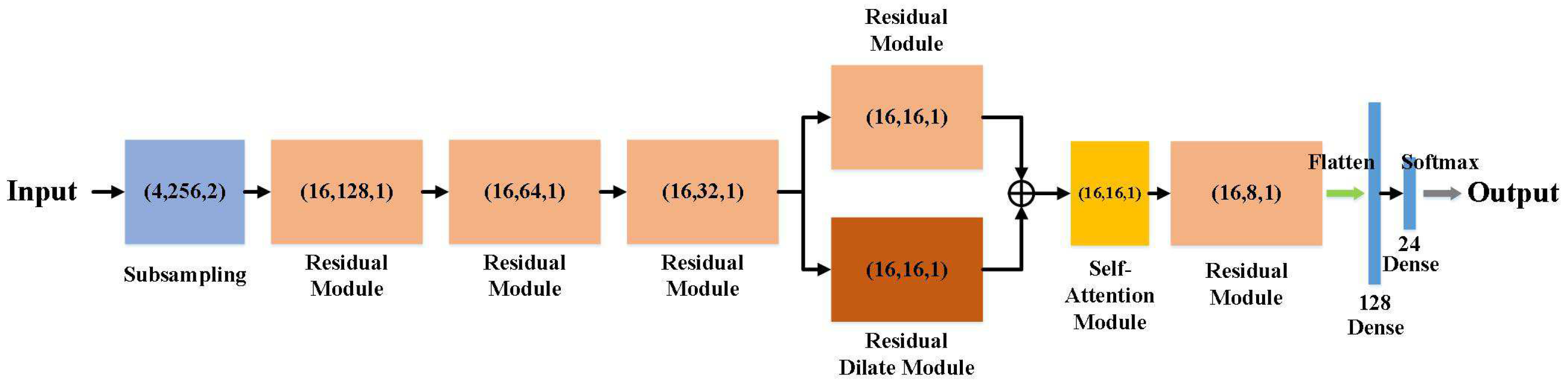
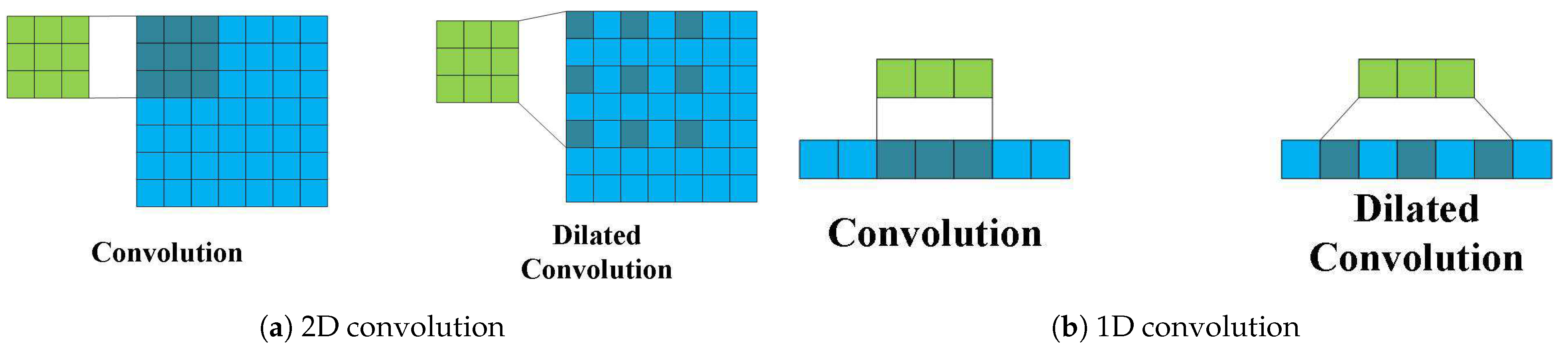
- We design an information integration module with ordinary convolution and dilated convolution branches. Dilated convolution has a larger receptive field than ordinary convolution and is more suitable for global information extraction. The sum of the two branches provides more detailed information.
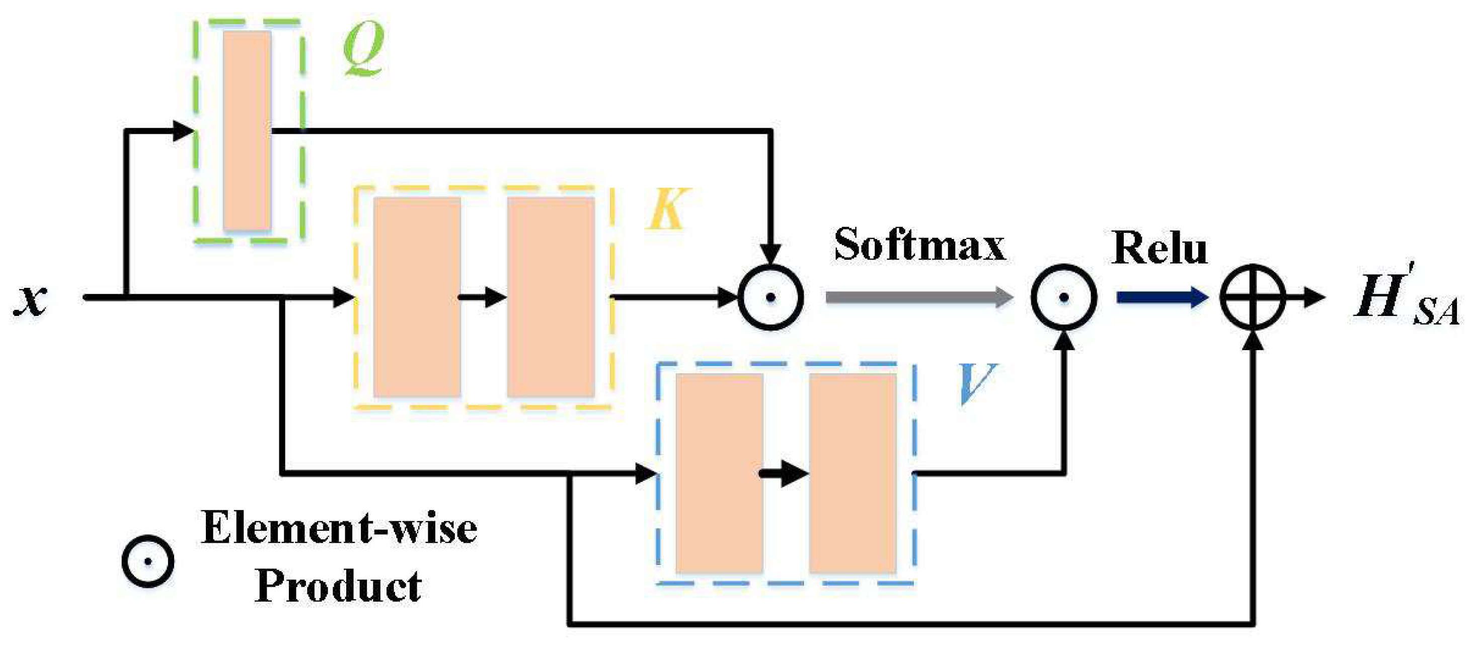
- To enhance the noise resistance, we introduce a self-attention module with a strong feature extraction capability. The module can dynamically adjust the weights of parameters to amplify the influence of those that are beneficial for modulation recognition and diminish the influence of invalid parameters during the recognition process.
- We subsample the signal into multiple signals with two branches, I and Q, and concatenate them channel-wise. We finesse the model architecture to prevent overfitting. We propose MSSAs in large, medium, and small sizes, with fewer parameters and faster speeds, which are more suitable for our UAV-to-ground AMR system.
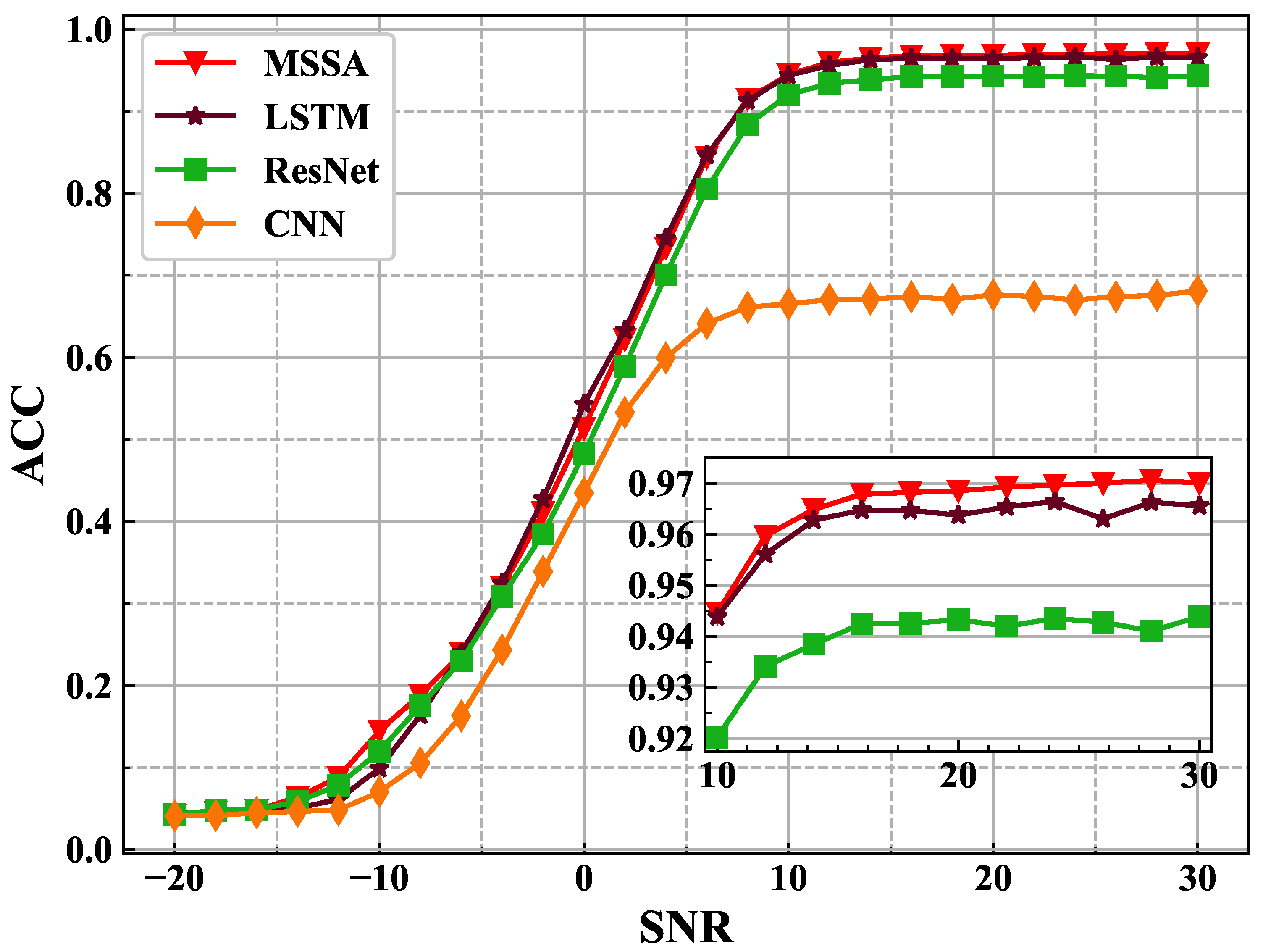
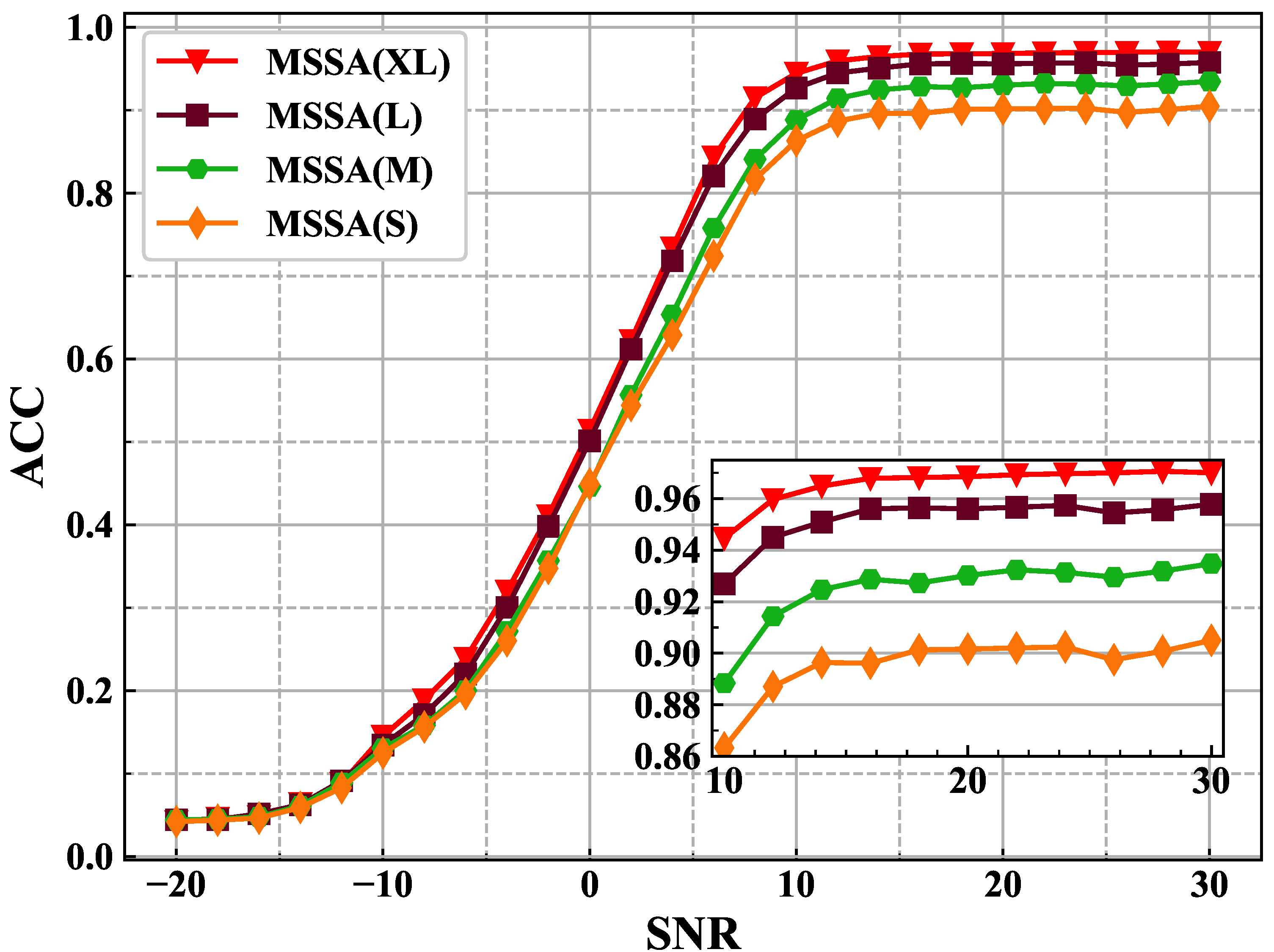
- Ablation experiments on a common dataset with current models show the ability of the proposed method in AMR. MSSA has the best performance on RML 2018.01a and accuracy when the signal-to-noise ratio (SNR) is 30 dB. Different sizes of MSSA each have their advantages in terms of accuracy, speed, and parameters. The weight file of MSSA(S) is only 652 KB.
1.3. Organization
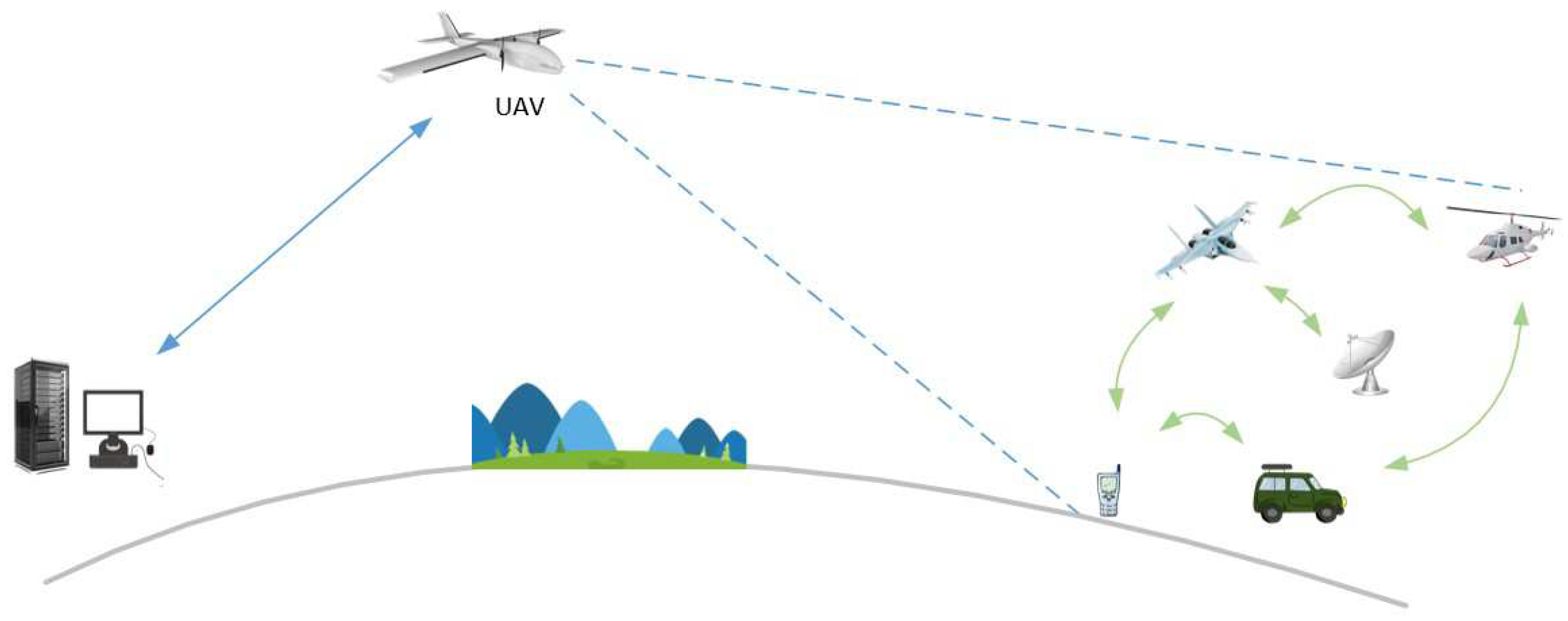
2. System Model
3. Design and Implementation of Multi-Subsampling Self-Attention Network
3.1. Architecture
3.2. Methodology
3.2.1. Enhanced Processing Range via Dilated Residual Connections
3.2.2. Enhanced Robustness of Attention Models against Noise
3.2.3. Streamlined Modeling with Subsampling Layer
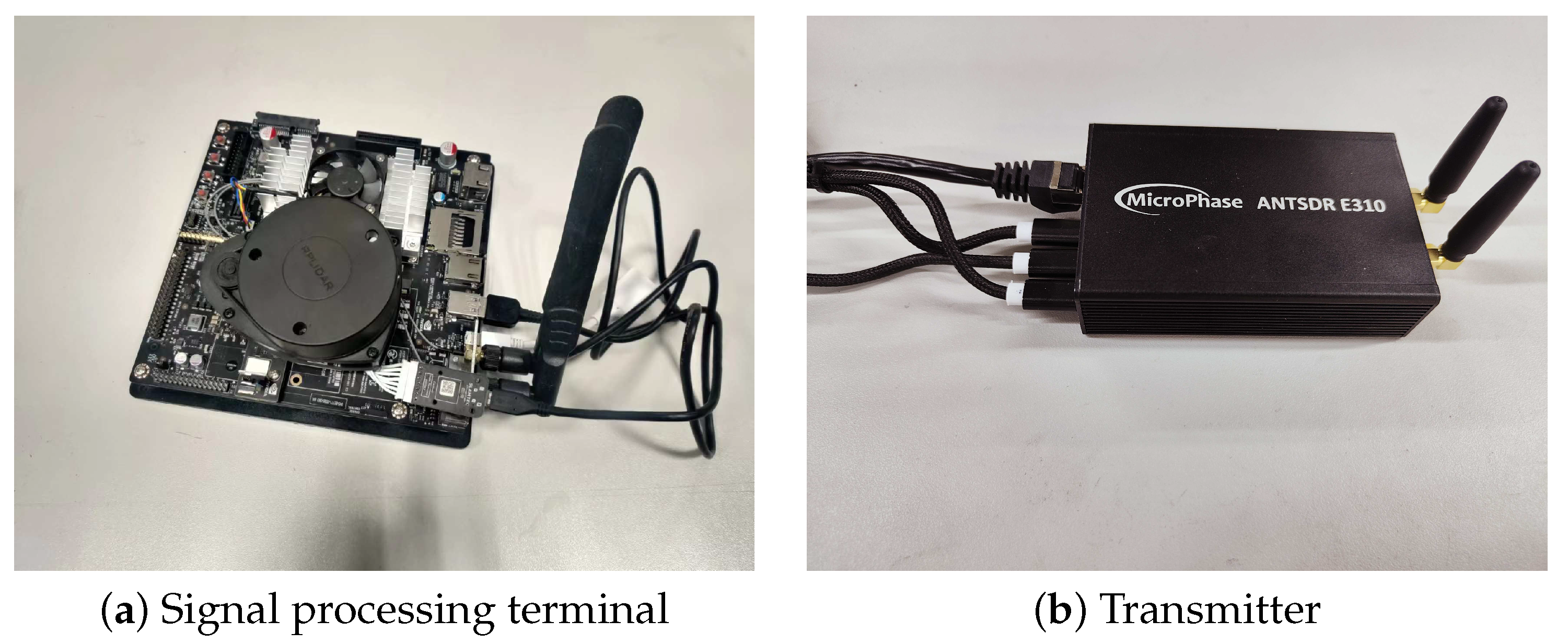
3.3. Equipment and Facilities
4. Experiments and Results
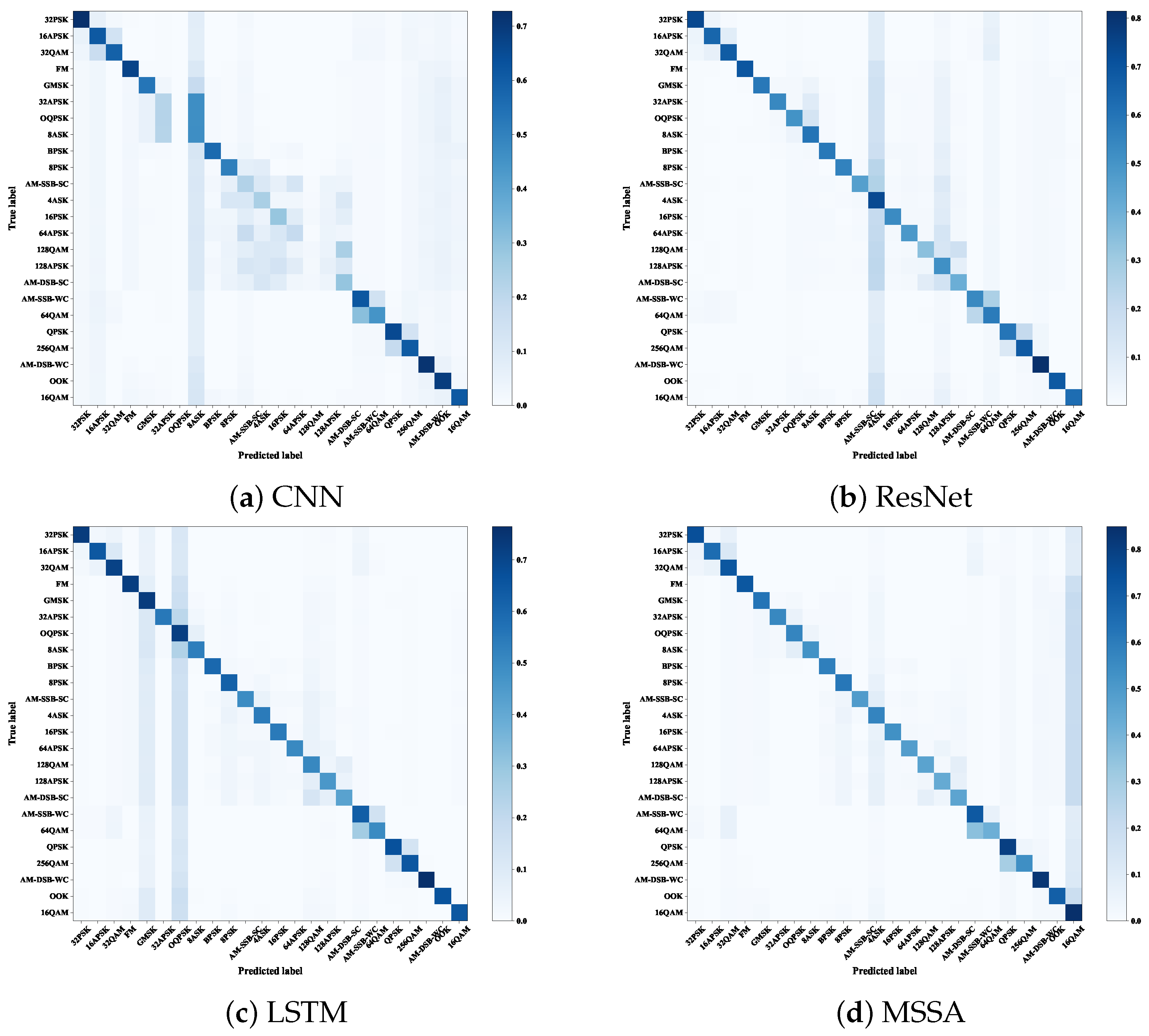
4.1. Experimental Comparison for AMR Task
4.2. Experimental Comparison on Hyperparameters
5. Conclusions
Author Contributions
Funding
Data Availability Statement
Conflicts of Interest
References
- Zhang, F.; Luo, C.; Xu, J.; Luo, Y.; Zheng, F. Deep Learning Based Automatic Modulation Recognition: Models, Datasets, and Challenges. Digit. Signal Process. 2022, 129, 103650. [Google Scholar] [CrossRef]
- Bhatti, F.A.; Khan, M.J.; Selim, A.; Paisana, F. Shared Spectrum Monitoring Using Deep Learning. IEEE Trans. Cogn. Commun. Netw. 2021, 7, 1171–1185. [Google Scholar] [CrossRef]
- Dobre, O.; Abdi, A.; Bar-Ness, Y.; Su, W. Survey of automatic modulation classification techniques: Classical approaches and new trends. IET Commun. 2007, 1, 137–156. [Google Scholar] [CrossRef] [Green Version]
- Zhang, W.; Feng, M.; Krunz, M.; Hossein Yazdani Abyaneh, A. Signal Detection and Classification in Shared Spectrum: A Deep Learning Approach. In Proceedings of the IEEE Conference on Computer Communications (IEEE INFOCOM 2021), Vancouver, BC, Canada, 10–13 May 2021; IEEE Press: Piscataway, NJ, USA, 2021; pp. 1–10. [Google Scholar] [CrossRef]
- Dulek, B. Online Hybrid Likelihood Based Modulation Classification Using Multiple Sensors. IEEE Trans. Wirel. Commun. 2017, 16, 4984–5000. [Google Scholar] [CrossRef]
- Xu, J.L.; Su, W.; Zhou, M. Likelihood-Ratio Approaches to Automatic Modulation Classification. IEEE Trans. Syst. Man Cybern. Part C Appl. Rev. 2011, 41, 455–469. [Google Scholar] [CrossRef]
- Hazza, A.; Shoaib, M.; Alshebeili, S.A.; Fahad, A. An overview of feature-based methods for digital modulation classification. In Proceedings of the 2013 1st International Conference on Communications, Signal Processing, and Their Applications (ICCSPA), Sharjah, United Arab Emirates, 12–14 February 2013; pp. 1–6. [Google Scholar] [CrossRef]
- Chan, Y.; Gadbois, L.; Yansouni, P. Identification of the modulation type of a signal. In Proceedings of the IEEE International Conference on Acoustics, Speech, and Signal Processing (ICASSP ’85), Tampa, FL, USA, 26–29 April 1985; Volume 10, pp. 838–841. [Google Scholar] [CrossRef]
- Hong, L.; Ho, K. Identification of digital modulation types using the wavelet transform. In Proceedings of the IEEE Military Communications Conference (MILCOM 1999), Atlantic City, NJ, USA, 31 October–3 November 1999; Cat. No.99CH36341. Volume 1, pp. 427–431. [Google Scholar] [CrossRef]
- Liu, L.; Xu, J. A Novel Modulation Classification Method Based on High Order Cumulants. In Proceedings of the 2006 International Conference on Wireless Communications, Networking and Mobile Computing, Wuhan, China, 22–24 September 2006; pp. 1–5. [Google Scholar] [CrossRef]
- Swami, A.; Sadler, B. Hierarchical digital modulation classification using cumulants. IEEE Trans. Commun. 2000, 48, 416–429. [Google Scholar] [CrossRef]
- Yuan, J.; Zhao-Yang, Z.; Pei-Liang, Q. Modulation classification of communication signals. In Proceedings of the Military Communications Conference (IEEE MILCOM 2004), Monterey, CA, USA, 31 October–3 November 2004; Volume 3, pp. 1470–1476. [Google Scholar] [CrossRef]
- Park, C.S.; Choi, J.H.; Nah, S.P.; Jang, W.; Kim, D.Y. Automatic Modulation Recognition of Digital Signals using Wavelet Features and SVM. In Proceedings of the 2008 10th International Conference on Advanced Communication Technology, Gangwon, Republic of Korea, 17–20 February 2008; Volume 1, pp. 387–390. [Google Scholar] [CrossRef]
- O’Shea, T.J.; Corgan, J.; Clancy, T.C. Convolutional Radio Modulation Recognition Networks. In Proceedings of the 17th International Conference (EANN 2016), Aberdeen, UK, 2–5 September 2016. [Google Scholar]
- Rajendran, S.; Meert, W.; Giustiniano, D.; Lenders, V.; Pollin, S. Deep Learning Models for Wireless Signal Classification with Distributed Low-Cost Spectrum Sensors. IEEE Trans. Cogn. Commun. Netw. 2018, 4, 433–445. [Google Scholar] [CrossRef] [Green Version]
- O’Shea, T.J.; Roy, T.; Clancy, T.C. Over-the-Air Deep Learning Based Radio Signal Classification. IEEE J. Sel. Top. Signal Process. 2018, 12, 168–179. [Google Scholar] [CrossRef] [Green Version]
- Njoku, J.N.; Morocho-Cayamcela, M.E.; Lim, W. CGDNet: Efficient Hybrid Deep Learning Model for Robust Automatic Modulation Recognition. IEEE Netw. Lett. 2021, 3, 47–51. [Google Scholar] [CrossRef]
- Hu, S.; Pei, Y.; Liang, P.P.; Liang, Y.C. Deep Neural Network for Robust Modulation Classification Under Uncertain Noise Conditions. IEEE Trans. Veh. Technol. 2020, 69, 564–577. [Google Scholar] [CrossRef]
- Zhang, M.; Zeng, Y.; Han, Z.; Gong, Y. Automatic Modulation Recognition Using Deep Learning Architectures. In Proceedings of the 2018 IEEE 19th International Workshop on Signal Processing Advances in Wireless Communications (SPAWC), Kalamata, Greece, 25–28 June 2018; pp. 1–5. [Google Scholar] [CrossRef]
- Ghasemzadeh, P.; Hempel, M.; Sharif, H. GS-QRNN: A High-Efficiency Automatic Modulation Classifier for Cognitive Radio IoT. IEEE Internet Things J. 2022, 9, 9467–9477. [Google Scholar] [CrossRef]
- Wang, T.; Hou, Y.; Zhang, H.; Guo, Z. Deep Learning Based Modulation Recognition With Multi-Cue Fusion. IEEE Wirel. Commun. Lett. 2021, 10, 1757–1760. [Google Scholar] [CrossRef]
- Li, Y.; Shao, G.; Wang, B. Automatic Modulation Classification Based on Bispectrum and CNN. In Proceedings of the 2019 IEEE 8th Joint International Information Technology and Artificial Intelligence Conference (ITAIC), Chongqing, China, 24–26 May 2019; pp. 311–316. [Google Scholar] [CrossRef]
- Peng, S.; Jiang, H.; Wang, H.; Alwageed, H.; Zhou, Y.; Sebdani, M.M.; Yao, Y.D. Modulation Classification Based on Signal Constellation Diagrams and Deep Learning. IEEE Trans. Neural Netw. Learn. Syst. 2019, 30, 718–727. [Google Scholar] [CrossRef] [PubMed]
- Krizhevsky, A.; Sutskever, I.; Hinton, G.E. ImageNet classification with deep convolutional neural networks. Commun. ACM 2012, 60, 84–90. [Google Scholar] [CrossRef] [Green Version]
- Szegedy, C.; Liu, W.; Jia, Y.; Sermanet, P.; Reed, S.; Anguelov, D.; Erhan, D.; Vanhoucke, V.; Rabinovich, A. Going Deeper with Convolutions. arXiv 2014, arXiv:1409.4842. [Google Scholar]
- Ramjee, S.; Ju, S.; Yang, D.; Liu, X.; Gamal, A.E.; Eldar, Y.C. Fast Deep Learning for Automatic Modulation Classification. arXiv 2019, arXiv:1901.05850. [Google Scholar]
- Alsamhi, S.H.; Shvetsov, A.V.; Kumar, S.; Hassan, J.; Alhartomi, M.A.; Shvetsova, S.V.; Sahal, R.; Hawbani, A. Computing in the Sky: A Survey on Intelligent Ubiquitous Computing for UAV-Assisted 6G Networks and Industry 4.0/5.0. Drones 2022, 6, 177. [Google Scholar] [CrossRef]
- Hu, X.; Wong, K.K.; Yang, K.; Zheng, Z. UAV-Assisted Relaying and Edge Computing: Scheduling and Trajectory Optimization. IEEE Trans. Wirel. Commun. 2019, 18, 4738–4752. [Google Scholar] [CrossRef]
- He, Y.; Wang, D.; Huang, F.; Zhang, R.; Gu, X.; Pan, J. A V2I and V2V Collaboration Framework to Support Emergency Communications in ABS-Aided Internet of Vehicles. IEEE Trans. Green Commun. Netw. 2023; early access. [Google Scholar] [CrossRef]
- Shi, J.; Zhao, L.; Wang, X.; Guizani, M.; Gaanin, H.; Lin, N. Flying Social Networks: Architecture, Challenges and Open Issues. IEEE Netw. 2021, 35, 242–248. [Google Scholar] [CrossRef]
- Ke, Z.; Vikalo, H. Real-Time Radio Technology and Modulation Classification via an LSTM Auto-Encoder. IEEE Trans. Wirel. Commun. 2022, 21, 370–382. [Google Scholar] [CrossRef]
- Chang, S.; Huang, S.; Zhang, R.; Feng, Z.; Liu, L. Multitask-Learning-Based Deep Neural Network for Automatic Modulation Classification. IEEE Internet Things J. 2022, 9, 2192–2206. [Google Scholar] [CrossRef]
- Srivastava, R.K.; Greff, K.; Schmidhuber, J. Training Very Deep Networks. In Proceedings of the Advances in Neural Information Processing Systems 28 (NIPS 2015) Conference, Montreal, QC, Canada, 7–12 December 2015; Cortes, C., Lawrence, N., Lee, D., Sugiyama, M., Garnett, R., Eds.; Curran Associates, Inc.: Red Hook, NY, USA, 2015; Volume 28, pp. 2377–2385. [Google Scholar]
- Vaswani, A.; Shazeer, N.; Parmar, N.; Uszkoreit, J.; Jones, L.; Gomez, A.N.; Kaiser, L.; Polosukhin, I. Attention Is All You Need. In Proceedings of the Advances in Neural Information Processing Systems 30 (NIPS 2017) Conference, Long Beach, CA, USA, 4–9 December 2017. [Google Scholar]


| Hyperparameters | Inputs | Residual | Residual Module | Dense |
|---|---|---|---|---|
| Shape | Modules | Filters | Units | |
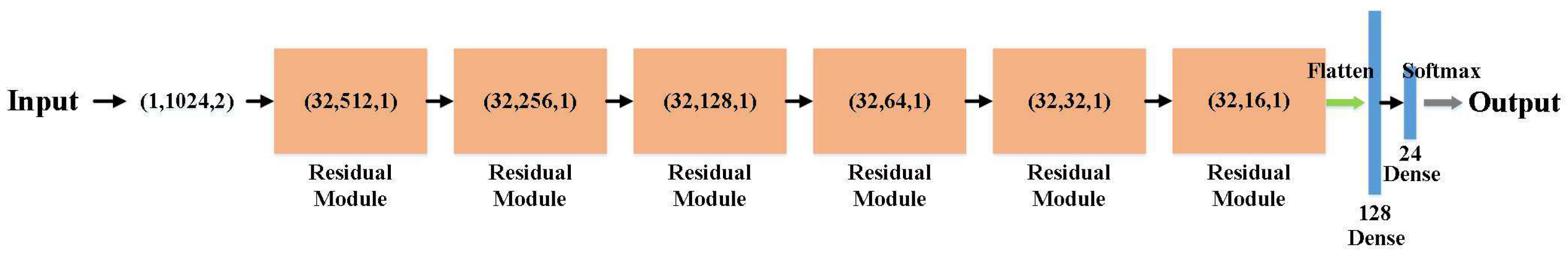
| MSSA(XL) | (1, 1024, 2) | 6 | 32 | 128 |
| MSSA(L) | (2, 512, 2) | 6 | 32 | 128 |
| MSSA(M) | (4, 256, 2) | 5 | 16 | 128 |
| MSSA(S) | (4, 256, 2) | 5 | 16 | 64 |
| Dataset | Number of Modulation Schemes | Sample Dimension | Dataset Size | SNR Range (dB) |
|---|---|---|---|---|
| RML 2016.04c | 11 | 162,060 | −20:2:18 | |
| RML 2016.10a | 11 | 220,000 | −20:2:18 | |
| RML 2016.10b | 10 | 1,200,000 | −20:2:18 | |
| RML 2018.01a | 24 | 2,555,904 | −20:2:30 |
| Acc (%) in SNR (dB) | 6 | 14 | 22 | 30 | Mean (−20:2:30) |
|---|---|---|---|---|---|
| CNN | 64.16 | 67.14 | 67.43 | 68.12 | 43.89 |
| ResNet | 80.54 | 93.85 | 94.20 | 94.39 | 58.81 |
| LSTM | 84.65 | 96.28 | 96.54 | 96.59 | 60.22 |
| MSSA | 84.38 | 96.49 | 96.93 | 97.00 | 60.90 |
| Time (Second/Epoch) | Parameters | SNR = 6 (dB) Acc (%) | SNR = 30 (dB) Acc (%) | Mean Acc (%) | |
|---|---|---|---|---|---|
| CNN | 367 | 13,064,524 | 64.16 | 68.12 | 43.89 |
| ResNet | 171 | 139,192 | 80.54 | 94.39 | 58.81 |
| LSTM | 1242 | 202,766 | 84.65 | 96.59 | 60.22 |
| MSSA(XL) | 283 | 218,200 | 84.38 | 97.00 | 60.90 |
| MSSA(L) | 171 | 152,696 | 82.09 | 95.78 | 59.70 |
| MSSA(M) | 99 | 54,632 | 75.80 | 93.48 | 57.01 |
| MSSA(S) | 99 | 36,648 | 72.43 | 90.50 | 55.25 |
Disclaimer/Publisher’s Note: The statements, opinions and data contained in all publications are solely those of the individual author(s) and contributor(s) and not of MDPI and/or the editor(s). MDPI and/or the editor(s) disclaim responsibility for any injury to people or property resulting from any ideas, methods, instructions or products referred to in the content. |
© 2023 by the authors. Licensee MDPI, Basel, Switzerland. This article is an open access article distributed under the terms and conditions of the Creative Commons Attribution (CC BY) license (https://creativecommons.org/licenses/by/4.0/).
Share and Cite
Shen, Y.; Yuan, H.; Zhang, P.; Li, Y.; Cai, M.; Li, J. A Multi-Subsampling Self-Attention Network for Unmanned Aerial Vehicle-to-Ground Automatic Modulation Recognition System. Drones 2023, 7, 376. https://doi.org/10.3390/drones7060376
Shen Y, Yuan H, Zhang P, Li Y, Cai M, Li J. A Multi-Subsampling Self-Attention Network for Unmanned Aerial Vehicle-to-Ground Automatic Modulation Recognition System. Drones. 2023; 7(6):376. https://doi.org/10.3390/drones7060376
Chicago/Turabian StyleShen, Yongjian, Hao Yuan, Pengyu Zhang, Yuheng Li, Minkang Cai, and Jingwen Li. 2023. "A Multi-Subsampling Self-Attention Network for Unmanned Aerial Vehicle-to-Ground Automatic Modulation Recognition System" Drones 7, no. 6: 376. https://doi.org/10.3390/drones7060376