


Deep Reinforcement Learning for the Visual Servoing Control of UAVs with FOV Constraint

Abstract
:1. Introduction
2. Preliminaries
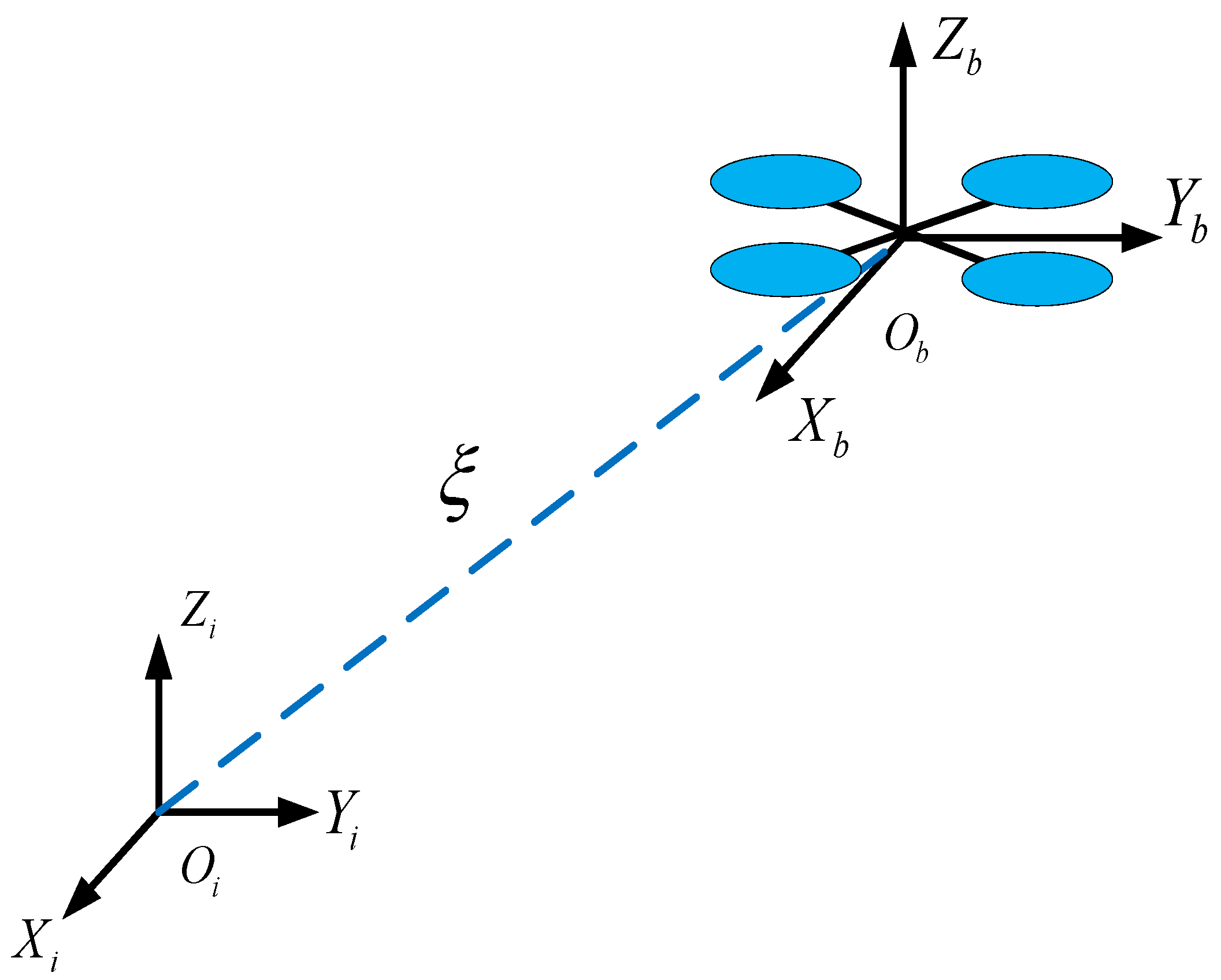
2.1. Quadrotor Model Description
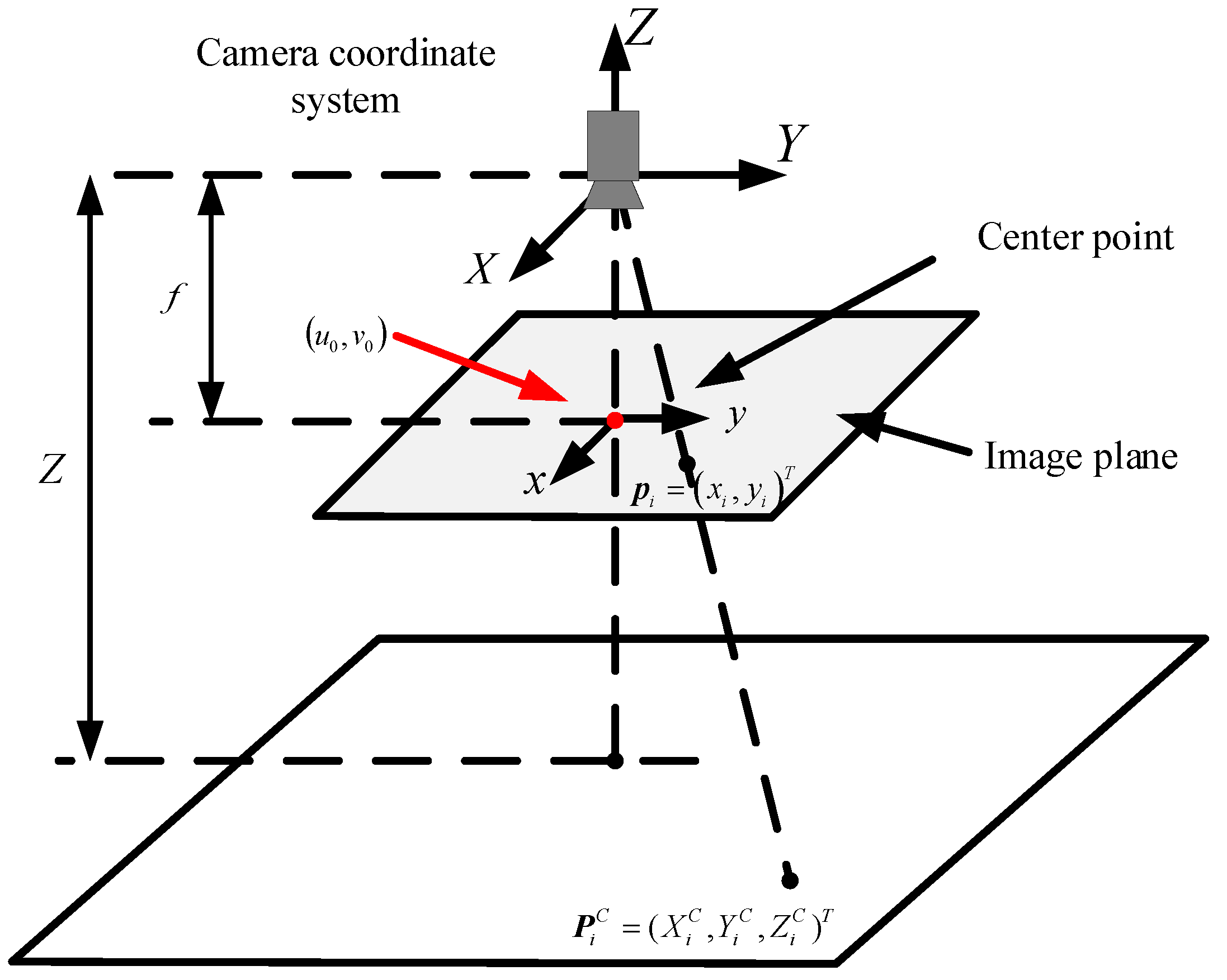
2.2. The Classical IBVS Method
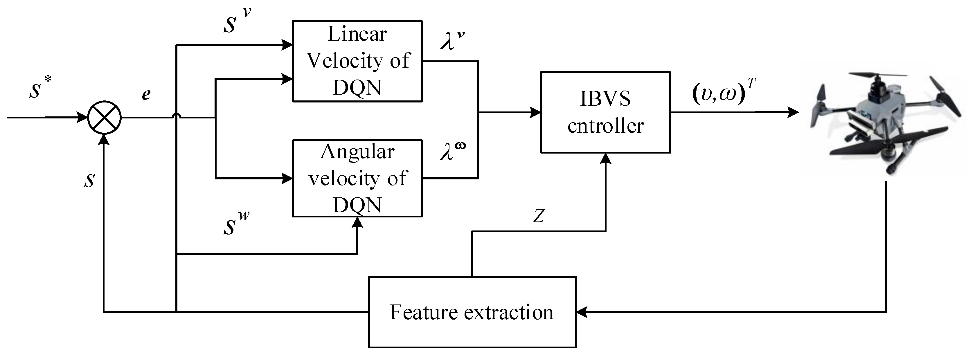
3. IBVS with Deep Reinforcement Learning
3.1. The Markov Decision Process Model
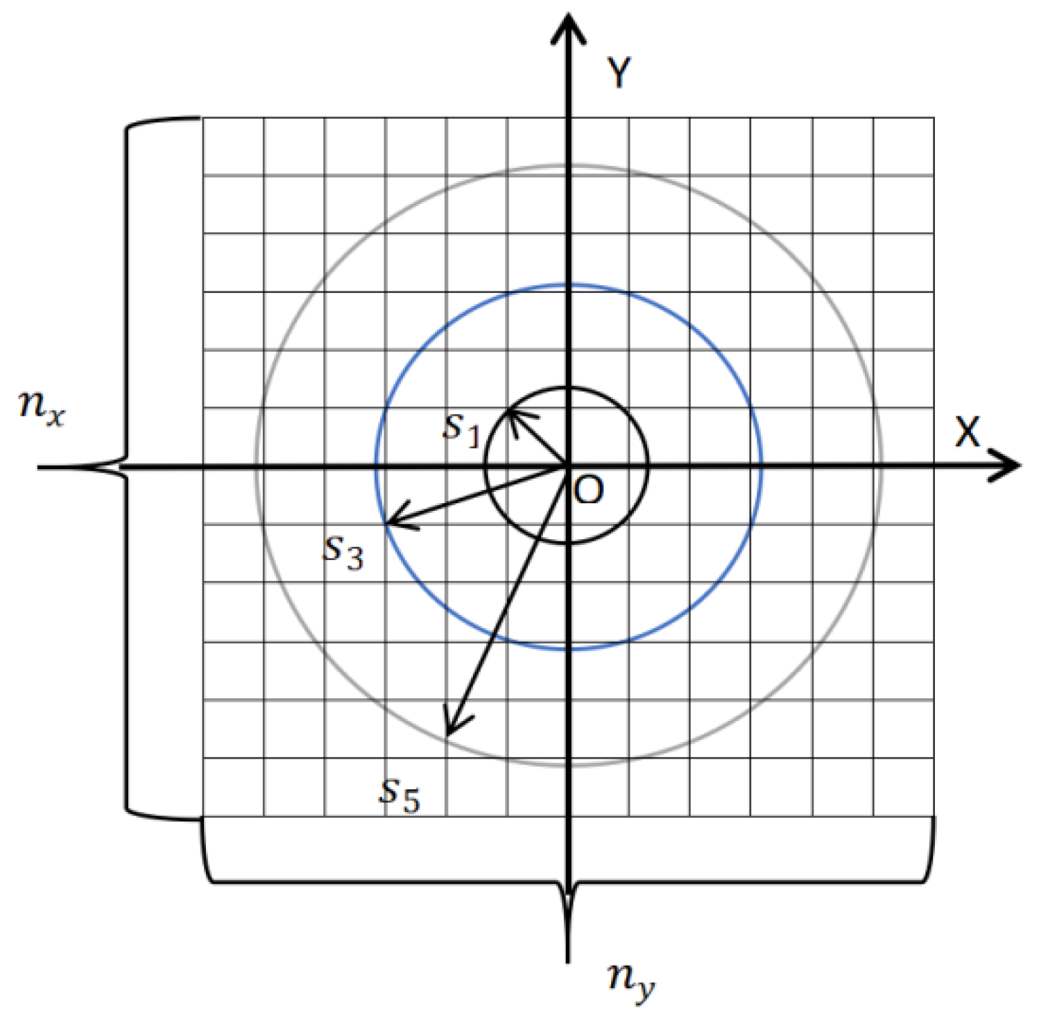
- State Space
- Action Selection
- Reward Function
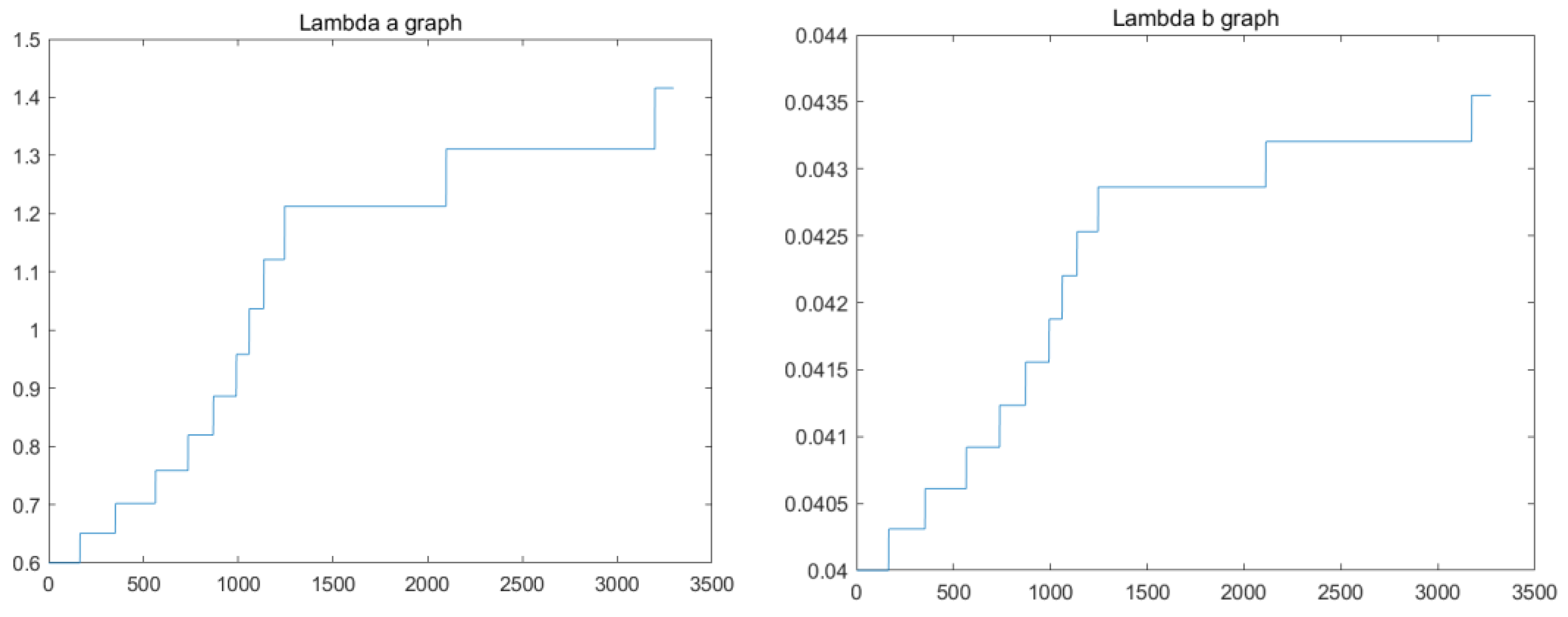
3.2. DQN Algorithm
- Target Network: With only one network, updating the Q function in real time can result in a chaotic trajectory and poor training. To avoid instability caused by updating the Q function while simultaneously acquiring the Q value, a target network is used. The target network provides a stable Q value for the Q function to be updated. The target network is updated with the new Q function to improve performance.
- Experience Replays: Experience replays will build a replay buffer . The replay buffer is also called replay memory. Instead of using the samples in the standard sequence, small batches are randomly selected from the data set for training to diminish the relativity between training samples.
| Algorithm 1: DQN-based IBVS method |
| Initialization; For episode = 1: For = 1: If or (Termination condition); Break End Generate random number:; If < Random selection of action ; Else Select the corresponding strategic actions ; obtain the rewards , and servo gains and ; and are substituted to ; Observe the next State ; Store the experience replay with ; ; End If Experience replay full Randomly selected datasets of buffer ; Train the network by gradient descent method and updating network parameters according to (24); After training a certain number of times, update the target network according to (25); End End End |
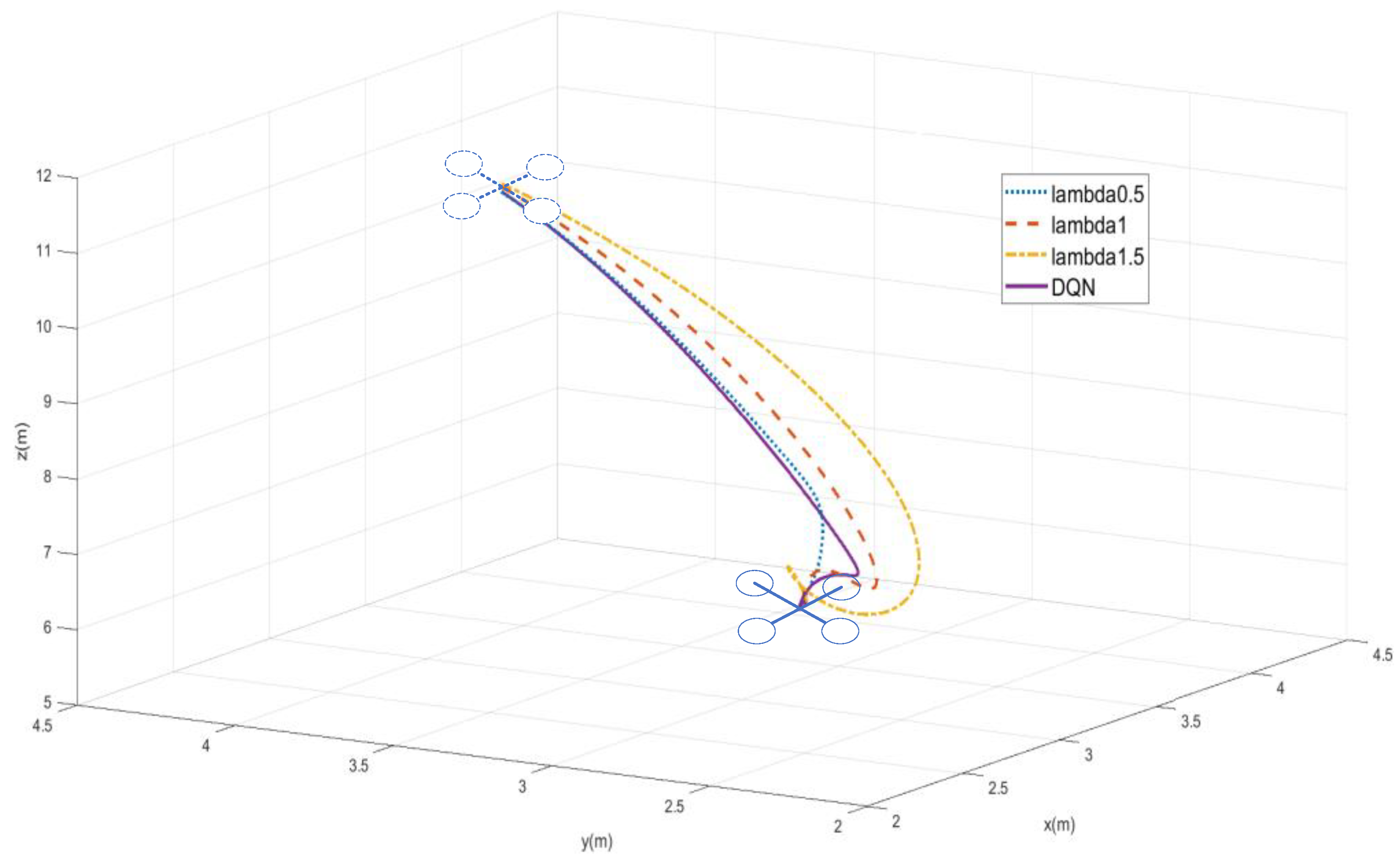
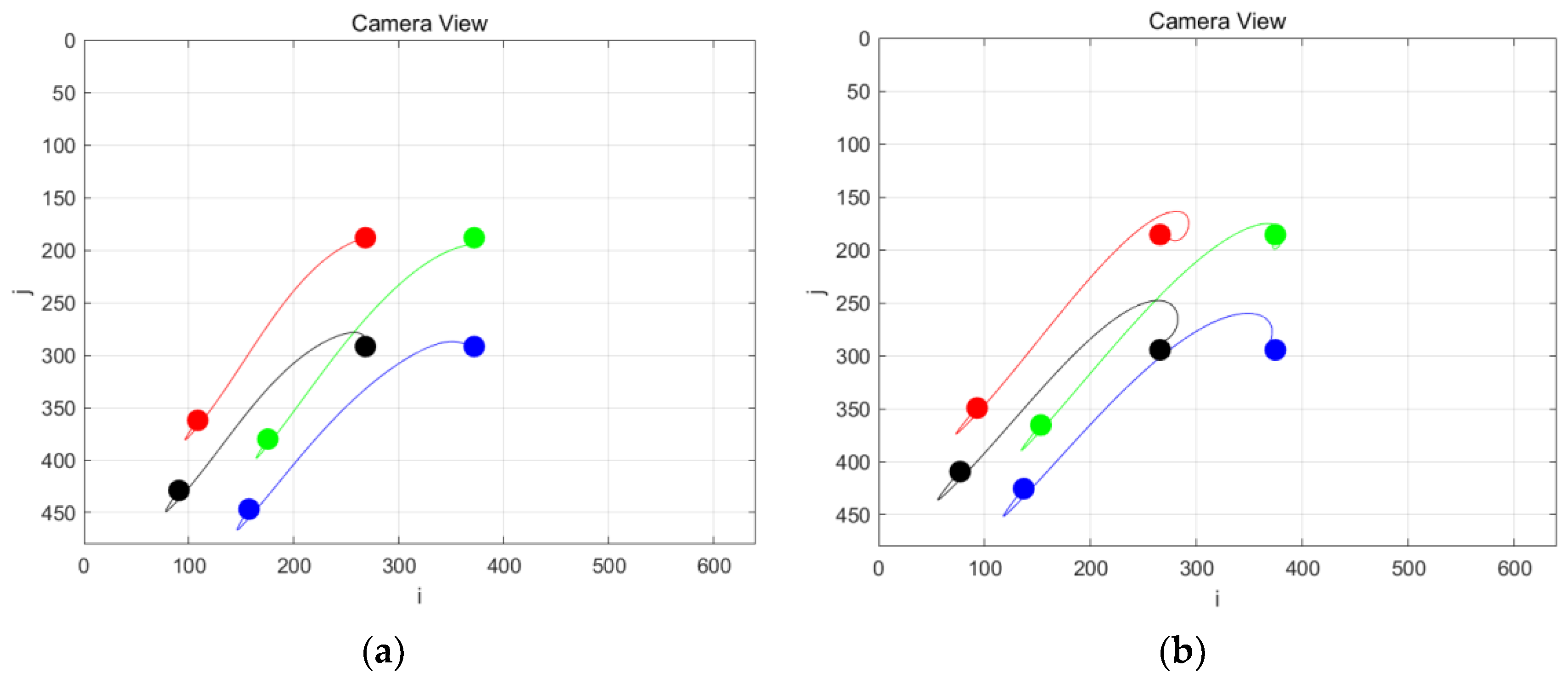
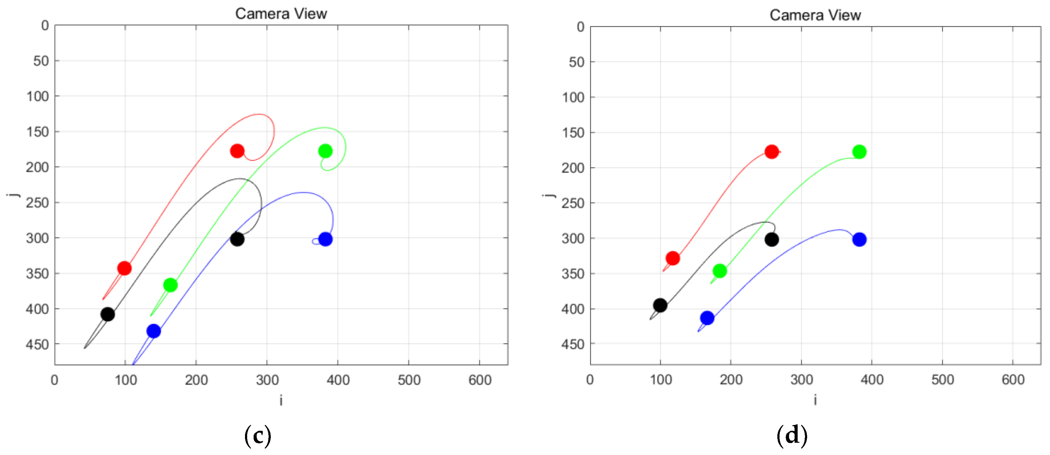
4. Simulations and Experiments
5. Conclusions
Author Contributions
Funding
Institutional Review Board Statement
Informed Consent Statement
Data Availability Statement
Conflicts of Interest
Abbreviations
| UAV | unmanned aerial vehicle |
| FOV | field of view |
| DRL | deep reinforcement learning |
| DQN | deep Q-network |
| PBVS | position-based visual servoing |
| IBVS | image-based visual servoing |
| WMRs | wheeled mobile robots |
| MPC | model predictive control |
References
- Alzahrani, B.; Oubbati, O.S.; Barnawi, A.; Atiquzzaman, M.; Alghazzawi, D. UAV assistance paradigm: State-of-the-art in applications and challenges. J. Netw. Comput. Appl. 2020, 166, 102706. [Google Scholar] [CrossRef]
- Mahony, R.; Kumar, V.; Corke, P. Multirotor Aerial Vehicles: Modeling, Estimation, and Control of Quadrotor. IEEE Robot. Autom. Mag. 2012, 19, 20–32. [Google Scholar] [CrossRef]
- Zhen, Z.; Chen, Y.; Wen, L.; Han, B. An intelligent cooperative mission planning scheme of UAV swarm in uncertain dynamic environment. Aerosp. Sci. Technol. 2020, 100, 105826. [Google Scholar] [CrossRef]
- Liu, Y.; Liu, H.; Tian, Y.; Sun, C. Reinforcement learning based two-level control framework of UAV swarm for cooperative persistent surveillance in an unknown urban area. Aerosp. Sci. Technol. 2020, 98, 105671. [Google Scholar] [CrossRef]
- Wu, Y.; Hu, X. An online route planning method for multi-rotor drone in urban environments. Control. Decis. 2021, 36, 2851–2860. [Google Scholar]
- Zheng, D.; Wang, H.; Wang, J.; Chen, S.; Chen, W.; Liang, X. Image-Based Visual servoing of a quadrotor using virtual camera approach. IEEE/ASME Trans. Mechatron. 2017, 22, 972–982. [Google Scholar] [CrossRef]
- Chaumette, F.; Hutchinson, S. Visual servo control. I. Basic approaches. IEEE Robot. Autom. Mag. 2006, 13, 82–90. [Google Scholar] [CrossRef]
- Chen, C.; Tian, Y.; Lin, L.; Chen, S.; Li, H.; Wang, Y.; Su, K. Obtaining World Coordinate Information of UAV in GNSS Denied Environments. Sensors 2020, 20, 2241. [Google Scholar] [CrossRef]
- Abdessameud, A.; Janabi-Sharifi, F. Image-based tracking control of VTOL unmanned aerial vehicles. Automatica 2015, 53, 111–119. [Google Scholar] [CrossRef]
- Zhang, X.; Fang, Y.; Li, B.; Wang, J. Visual servoing of nonholonomic mobile robots with uncalibrated Camera-to-Robot parameters. IEEE Trans. Ind. Electron. 2017, 64, 390–400. [Google Scholar] [CrossRef]
- Zhang, X.; Fang, Y.; Zhang, X.; Jiang, J.; Chen, X. Dynamic Image-Based Output Feedback Control for Visual Servoing of Multirotors. IEEE Trans. Ind. Inform. 2020, 16, 7624–7636. [Google Scholar] [CrossRef]
- Ceren, Z.; Altuğ, E. Image based and hybrid visual servo control of an unmanned aerial vehicle. J. Intell. Robot. Syst. 2012, 65, 325–344. [Google Scholar] [CrossRef]
- Liu, N.; Shao, X.; Yang, W. Desired compensation RISE-based IBVSS control of quadrotor for tracking a moving target. Nonlinear Dyn. 2019, 95, 2605–2624. [Google Scholar] [CrossRef]
- Santamaria-Navarro, À.; Andrade-Cetto, J. Uncalibrated image based visual servoing. In Proceedings of the 2013 IEEE International Conference on Robotics and Automation, Karlsruhe, Germany, 6–10 May 2013; pp. 5247–5252. [Google Scholar]
- Miao, Z.; Zhong, H.; Lin, J.; Wang, Y.; Chen, Y.; Fierro, R. Vision-Based Formation Control of Mobile Robots With FOV Constraints and Unknown Feature Depth. IEEE Trans. Control. Syst. Technol. 2021, 29, 2231–2238. [Google Scholar] [CrossRef]
- Lopez-Nicolas, G.; Aranda, M.; Mezouar, Y. Formation of differential-drive vehicles with field-of-view constraints for enclosing a moving target. In Proceedings of the 2017 IEEE International Conference on Robotics and Automation (ICRA), Singapore, Singapore, 29 May–3 June 2017; IEEE: Piscataway, NJ, USA, 2017; pp. 261–266. [Google Scholar]
- Bhagat, S.; Pb, S. UAV Target Tracking in Urban Environments Using Deep Reinforcement Learning. In Proceedings of the 2020 International Conference on Unmanned Aircraft Systems (ICUAS), Athens, Greece, 1–4 September 2020. [Google Scholar]
- Bruno, H.M.S.; Colombini, E.L. LIFT-SLAM: A deep-learning feature-based monocular visual SLAM method. Neurocomputing 2021, 455, 97–110. [Google Scholar] [CrossRef]
- Hajiloo, A.; Keshmiri, M.; Xie, W.F.; Wang, T.T. Robust Online Model Predictive Control for a Constrained Image-Based Visual Servoing. IEEE Trans. Ind. Electron. 2016, 63, 2242–2250. [Google Scholar]
- Chesi, G. Visual Servoing Path Planning via Homogeneous Forms and LMI Optimizations. IEEE Trans. Robot. 2009, 25, 281–291. [Google Scholar] [CrossRef]
- Huang, Y.; Zhu, M.; Zheng, Z.; Low, K.H. Homography-based visual servoing for underactuated VTOL UAVs tracking a 6-DOF moving ship. IEEE Trans. Veh. Technol. 2022, 71, 2385–2398. [Google Scholar] [CrossRef]
- Zhang, X.; Fang, Y.; Zhang, X.; Shen, P.; Jiang, J.; Chen, X. Attitude-Constrained Time-Optimal Trajectory Planning for Rotorcrafts: Theory and Application to Visual Servoing. IEEE/ASME Trans. Mechatron. 2020, 25, 1912–1921. [Google Scholar] [CrossRef]
- Zheng, D.; Wang, H.; Wang, J.; Zhang, X.; Chen, W. Toward Visibility Guaranteed Visual Servoing Control of Quadrotor UAVs. IEEE/ASME Trans. Mechatron. 2019, 24, 1087–1095. [Google Scholar] [CrossRef]
- Krichen, M.; Mihoub, A.; Alzahrani, M.Y.; Adoni, W.Y.H.; Nahhal, T. Are Formal Methods Applicable To Machine Learning And Artificial Intelligence? In Proceedings of the 2022 2nd International Conference of Smart Systems and Emerging Technologies (SMARTTECH), Riyadh, Saudi Arabia, 9–11 May 2022; pp. 48–53. [Google Scholar]
- Seshia, S.A.; Sadigh, D.; Sastry, S.S. Toward Verified Artificial Intelligence. Commun. ACM 2022, 65, 46–55. [Google Scholar] [CrossRef]
- Sutton, R.S.; Barto, A.G. Reinforcement Learning: An Introduction; MIT Press: Cambridge, MA, USA, 2018. [Google Scholar]
- Wang, Y.; Lang, H.; De Silva, C.W. A Hybrid Visual Servo Controller for Robust Grasping by Wheeled Mobile Robots. IEEE/ASME Trans. Mechatron. 2010, 15, 757–769. [Google Scholar] [CrossRef]
- Shi, H.; Li, X.; Hwang, K.S.; Pan, W.; Xu, G. Decoupled visual servoing with fuzzy Q-learning. IEEE Trans. Ind. Inform. 2018, 14, 241–252. [Google Scholar] [CrossRef]
- Shi, H.; Shi, L.; Sun, G.; Hwang, K.S. Adaptive Image-Based Visual Servoing for Hovering Control of Quad-rotor. IEEE Trans. Cogn. Dev. Syst. 2020, 12, 417–426. [Google Scholar] [CrossRef]


| Reference | Object | Method |
|---|---|---|
| [19] | Six-DOF robot manipulator | The constraints due to actuator limitations and visibility constraints can be taken into account using MPC strategy and computational complexity. |
| [20] | Six-DOF articulated arm | Trajectory in the 3D space satisfying FOV constraints. It depends on accurate environmental and system models. |
| [21] | VTOL UAVs | Generate the constrained control inputs to ensure the nonsingular attitude extraction and FOV. |
| [22] | Quadrotor | FOV is indirectly guaranteed by attitude constraints. |
| [23] | Quadrotor | The system is bounded by a visible set. Control barrier function |
| [27] | WMRs | Using Q-learning to design a controller, the action is simple. |
| [28,29] | Quadrotor | Using Q-learning to design adaptive laws, the control effectiveness is improved without considering the FOV |
| Ours | Quadrotor | Using DQN to design adaptive laws, the control effectiveness is improved considering the FOV |
| Parameters | Value |
|---|---|
| 5 pixels | |
| 0.8 | |
| 0.9 | |
| 0.04 | |
| 0.6 | |
| episode | 500 |
Disclaimer/Publisher’s Note: The statements, opinions and data contained in all publications are solely those of the individual author(s) and contributor(s) and not of MDPI and/or the editor(s). MDPI and/or the editor(s) disclaim responsibility for any injury to people or property resulting from any ideas, methods, instructions or products referred to in the content. |
© 2023 by the authors. Licensee MDPI, Basel, Switzerland. This article is an open access article distributed under the terms and conditions of the Creative Commons Attribution (CC BY) license (https://creativecommons.org/licenses/by/4.0/).
Share and Cite
Fu, G.; Chu, H.; Liu, L.; Fang, L.; Zhu, X. Deep Reinforcement Learning for the Visual Servoing Control of UAVs with FOV Constraint. Drones 2023, 7, 375. https://doi.org/10.3390/drones7060375
Fu G, Chu H, Liu L, Fang L, Zhu X. Deep Reinforcement Learning for the Visual Servoing Control of UAVs with FOV Constraint. Drones. 2023; 7(6):375. https://doi.org/10.3390/drones7060375
Chicago/Turabian StyleFu, Gui, Hongyu Chu, Liwen Liu, Linyi Fang, and Xinyu Zhu. 2023. "Deep Reinforcement Learning for the Visual Servoing Control of UAVs with FOV Constraint" Drones 7, no. 6: 375. https://doi.org/10.3390/drones7060375