Path Planning of Autonomous Mobile Robots Based on an Improved Slime Mould Algorithm

Abstract

Path planning is a crucial component of autonomous mobile robot (AMR) systems. The slime mould algorithm (SMA), as one of the most popular path-planning approaches, shows excellent performance in the AMR field. Despite its advantages, there is still room for SMA to improve due to the lack of a mechanism for jumping out of local optimization. This means that there is still room for improvement in the path planning of ARM based on this method. To find shorter and more stable paths, an improved SMA, called the Lévy flight-rotation SMA (LRSMA), is proposed. LRSMA utilizes variable neighborhood Lévy flight and an individual rotation perturbation and variation mechanism to enhance the local optimization ability and prevent falling into local optimization. Experiments in varying environments demonstrate that the proposed algorithm can generate the ideal collision-free path with the shortest length, higher accuracy, and robust stability.

1. Introduction

With the rapid development of artificial intelligence technology, the intelligence and automation of autonomous mobile robots (AMRs) have advanced significantly. AMRs are widely used in many high-tech aspects, such as smart homes, intelligent logistics, and autonomous vehicles. Path planning, which is a crucial component of the AMR system, aims to generate a feasible, safe, and smooth path from the starting point to the target point in an unknown or known environment [1]. However, with the increasing types and scales of AMR applications, existing path-planning approaches cannot fulfill all demands due to constraints such as complexity and nonlinearity [2]. As a challenging research hotspot, it has attracted several studies on performance improvement in terms of effectiveness and efficiency [3].

Many traditional path-planning methods do not consider complexity and randomness, resulting in locally optimal solutions [4]. Meta-heuristic algorithms, on the other hand, utilize global search to find the best approximate solution by exploring and exploiting the overall search space [5]. Meta-heuristic algorithms can be categorized into evolutionary algorithms, such as simulated annealing, and swarm intelligence algorithms (SIAs), which simulate the behavior of biological groups in nature and exchange information and experience to solve global optimization problems [6].

In recent years, researchers have used many algorithms based on swarm intelligence to solve the path-planning problem of robots. Commonly used meta-heuristic algorithms include the genetic algorithm (GA) [7], particle swarm optimization (PSO) [8], ant colony optimization (ACO) [9], monarch butterfly optimization (MBO) [10], whale optimization algorithm (WOA) [11], grey wolf optimization (GWO) [12], and slime mould algorithm (SMA) [13]. SIAs are a combination of a stochastic algorithm and local search and perform well in solving highly nonlinear and multi-modal optimization problems [14]. However, SIAs still face some challenges, such as local optimization and slow convergence. GA simulates the evolution laws of the biological world. Although GA has great global optimization capability, it requires a large population and broad search space, which can result in local optimization and slow convergence in the search process [7]. In PSO, the flying process of particles is the individual’s search process. The flying speed of particles can be dynamically adjusted based on the individual’s historical best position and the population’s historical best position. PSO is prone to early convergence when solving complex optimization problems [13]. ACO divides the search space into grids in the field of path planning and utilizes the state transition probability and pheromone updating method to solve the algorithm [15]. However, the convergence speed of ACO can be slow, resulting in an extensive calculation [16]. MBO, WOA, and SMA are also known to experience slow local convergence, while GWO exhibits poor population diversity and slow convergence speed in later stages. In the robot path-planning field, PSO, WOA, GWO, and SMA are generally used algorithms for comparison. This paper will also compare these algorithms, which are common in mainstream practice.

The SMA is a meta-heuristic algorithm that was first proposed by Nagataki in 2000 [17]. It has been successfully applied to various areas, such as the selection of traffic network nodes [18], economic emission dispatch [19], robot path planning [20], medical image classification [21], and feature selection [22]. In 2020, Li et al. [23] proposed an SMA optimization for studying the activity and dynamics of slime moulds. Due to the excessive randomness in the meta-heuristic optimization process, it is essential to strike a proper balance between exploration and exploitation to optimize the algorithm effectively. In various studies, it has been found that SMA achieves excellent exploitation, while maintaining a significant balance with exploration. In multiple benchmark functions, SMA has shown outstanding performance compared to other algorithms, such as WOA, GWO, and PSO [14]. However, there is still limited research on using the SMA algorithm for AMR navigation. Additionally, in some cases or functions, SMA may present defects, such as failure to converge to the global optimal or slow convergence, and it may lack an effective escape mechanism.

This paper builds upon the work of Agarwal and Bharti [20] and proposes a path-planning algorithm called Lévy flight-rotation SMA (LRSMA) that updates the variable neighborhood Lévy mechanism to improve the algorithm’s convergence accuracy. It also introduces a real-time convergence stagnation monitoring strategy based on tolerance, which guides the population out of local optima using individual rotation perturbation and mutation mechanisms. The mobile robot considered in this paper is autonomous, a type of dynamic remotely operated navigation equipment (DRONE). Besides, it is easy to apply to other types of drones, such as aerial robots. The main contributions of this study are summarized as follows:

(a) A path-planning solution is proposed to generate the shortest no-collision curve path with robustness for AMRs.

(b) A perturbation mutation method based on rotation transformation is applied to increase the probability of finding the best solution near the suboptimal solution.

This paper is structured as follows. The first chapter introduces the research background, as mentioned above. The second chapter discusses related work. The third chapter introduces the SMA. The fourth chapter presents path planning based on the proposed LRSMA. The fifth chapter compares the LRSMA with other algorithms to verify its effectiveness in path planning. The last chapter provides the conclusion.

2. Related Work

Traditional path-planning algorithms, such as the A star algorithm [24], the artificial potential field method [25], the rapidly exploring random tree (RRT) algorithm [26], fuzzy logic [27], and neural networks [28], are widely used in robot path planning. However, these algorithms face challenges in complex environments due to poor adaptability and slow convergence. The A star algorithm requires prior information about the environment, which can optimize the path but is inefficient under large-scale complex conditions [24]. The artificial potential field method is often used in real-time dynamic environments but can easily fall into planning stagnation and local optimization in complex environments with obstacles [25]. The RRT can quickly search an unknown space and solve complex constraints with few parameters through a simple structure, but there are still issues in improving search efficiency and obtaining the optimal path [26]. The fuzzy logic algorithm is applied to handle scenarios with uncertain environment information, but the rule database needs to be updated frequently during path planning, and it has a high computational cost under complex conditions [27]. The neural network method does not require prior information about the environment and has broad applicability to real-time dynamic scenarios, but in complex environments with obstacles, the processing of massive networks results in a significant computational burden [28]. Although traditional path-planning algorithms have shown excellent performance in solving path planning under specific conditions [29], they cannot adequately satisfy the requirements for path planning in complex environments due to inadequate adaption, slow convergence, and other factors [30].

The path-planning problem can be transformed into the problem of finding the optimal path with the minimum cost function value [31]. Thanks to the optimization advantages in solving discontinuous, non-smooth, and discrete variable problems, SIAs have been commonly applied to path planning. Researchers are continuously improving these algorithms and exploring ones with higher planning efficiency, better optimization ability, and greater robustness [32].

For example, Wang et al. [33] proposed an ant colony path-planning algorithm in a 3D environment, which improves the global pheromone and designs a heuristic function with a safe value. This solves the problems of easily falling into local optimization and having a long search time in 3D path planning. Teng et al. [34] proposed a GWO based on PSO and used nonlinear control parameters to balance the local and global search. They also introduced PSO to update the positions of grey wolves, preventing the algorithm from falling into local optimization. Fernandes et al. [35] proposed a Quantum-behaved Particle Swarm Optimization (QPSO) algorithm that can produce a diverse population of peak values, effectively avoiding stagnation in the optimization process and solving path planning in both static and dynamic scenarios. Dai et al. [11] proposed an optimized WOA, adopted adaptive technology to improve the convergence speed, and set virtual obstacles and improved potential field factors to enhance the dynamic obstacle avoidance ability of AMRs. The WOA has a strong search ability despite its slow computation.

Slime molds belong to the Polycephalum family. The Physarum polycephalum algorithm requires numerous iterations and initial parameters, making it redundant for complex problems. The SMA proposed by Li et al. [23] simulates the behavior and morphological changes of Physarum polycephalum myxomycetes during foraging. The front end of slime molds is fan-shaped, and the back is an interconnected venous network. When the venous network approaches food, the biological oscillator of the slime mold produces a diffusion wave that changes the flow of cytoplasm in the vein, and the slime mold moves to a higher-quality food. The SMA adjusts search modes according to the fitness value. Additionally, slime molds will shrink to the optimal position and separate into multiple individuals to explore other spaces.

The SMA has strong global optimization due to a multiple exploration mechanism. It has diverse applications, such as the selection of traffic network nodes [18], robot path planning [20], medical image classification [21], and feature selection [22]. However, the SMA has unstable optimization and can easily fall into local optimization due to its simple optimization mechanism. Achievable improvements are applied to solve this problem, which can divide into three categories. The first is optimizing the population position update mechanism. Yu et al. [36] applied the quantum rotation gate and water cycle strategies, keeping the population balanced between exploration and exploitation, thus solving local optimization and slow convergence problems in later iterations. Nguyen et al. [37] proposed an improved SMA that adjusted the weight coefficient and introduced a reverse learning strategy to enhance optimization performance when updating the positions of slime molds. The second category is expanding the search space of the population. Rizk-Allah et al. [38] adopted the chaos-opposition-enhanced strategy to expand the search space and avoid premature algorithm convergence. Houssein et al. [39] integrated improved opposition-based learning and orthogonal learning mechanisms to prevent the algorithm from falling into local optimization due to rapid population assimilation. The third approach is introducing mutation operators. Houssein et al. [40] employed an adaptive guided differential evolution algorithm to improve the population’s local search ability, increase the population’s diversity, and avoid premature convergence. Liu and Liu [41] used quasi-reverse and quasi-reflective learning to expand the search space and introduce an unscented transformation sigma point to guide the search of the SMA, thereby solving the problems of search stagnation and poor stability.

While previous research has improved the performance of the SMA, optimizing the multi-objective function in path planning remains unsolved. Additionally, few studies have reported on robot path planning with obstacle avoidance in various environments. In other words, it is necessary to develop practical applications and further improvements in path planning. Hence, this paper proposes the LRSMA to achieve the shortest and collision-free path with robustness and efficiency for AMRs. The effectiveness and efficiency of the LRSMA are compared with those of the GWO, WOA, PSO, and SMA to validate its performance.

3. Overview of the SMA

The SMA uses a mathematical model to simulate the slime molds’ foraging behavior and morphological changes when approaching and surrounding food [23]. If slime molds find food while foraging, they generate interconnected vein networks of varying thicknesses between multiple food sources based on the quality and density of the food source. Slime molds spread into food, creating positive and negative feedback through diffusion waves, enabling them to search for higher-quality food. The whole process contains three stages.

• Approach food stage

Slime mold individuals approach food based on odor. Suppose the population of slime molds in a $D$-dimensional searching space is $N$. The updated position of a slime mold $X\left(t+1\right)$ at the $t$th iteration when approaching food can be expressed as follows:

$$X\left(t+1\right)=\left\{\begin{array}{l}X\_best\left(t\right)+vb\times (W\times X_{r1}\left(t\right)-X_{r2}\left(t\right)),{rand}_1<p,\\ vc\times X\left(t\right),{rand}_1\ge p,\end{array}\right.$$

(1)

where $t$ is the current iteration index, $X\left(t\right)$ is the position of a slime mold, and $X\left(t+1\right)$ is the new updated position of the slime mold. $X\_best\left(t\right)$ is the position of the best solution at the $t$th iteration. $X_{r1}\left(t\right)$ and $X_{r2}\left(t\right)$ are the positions of two slime molds randomly selected from the population. $vc$ is a control parameter that evaluates the changes in the use of historical data by slime molds, whose value decreases linearly from 1 to 0. ${rand}_1$ is a random number in the range [0, 1].

$p$ is a control parameter that determines the position update mode of slime molds and can be obtained as follows:

$$p=tanh\left|S\left(i\right)-DF\right|,i\in \left\{\mathrm{1,2},\dots ,N\right\},$$

(2)

where $i$ is the slime mold index, $S\left(i\right)$ is the fitness of the $i$th slime mold, and $DF$ is the fitness of the best solution.

$vb$ is a random number in the range [−$a$, $a$] regarded as a control parameter; its value range decreases with the decrease in $a$. Parameter $a$, used to simulate the gradual and dynamic contraction of veins when slime molds approach food, is expressed as follows:

$$a=arctanh\left(-\frac{t}{{IT}_{max}}+1\right),$$

(3)

where ${IT}_{max}$ is the maximum number of iterations.

The weight coefficient $W$ represents the oscillation frequency of the biological oscillator, which changes with food concentration when the slime molds approach food. If the food where the slime molds are located has a high concentration, there is positive feedback to the slime molds, and vice versa. $W$ is defined as

$$\left\{\begin{array}{l}W\left(SIndex\left(i\right)\right)=\left\{\begin{array}{c}{1+r}_2\times lg\left(\frac{bF-S\left(i\right)}{bF-wF}+1\right),condition,\hfill \\ {1-r}_2\times lg\left(\frac{bF-S\left(i\right)}{bF-wF}+1\right),others,\hfill \end{array}\right.\\ SIndex\left(i\right)=sort\left(N\right),\end{array}\right.$$

(4)

where $r_2$ is a random number in the range [0, 1]; $SIndex\left(i\right)$ is the sort index of the slime mold, and $bF$ and $wF$ indicate the best fitness and the worst fitness, respectively. $lg$ is used to reduce the change rate of the fitness, $condition$ indicates slime molds with the fitness ranking of the first half of the population, and $others$ denotes the remaining slime molds.

• Wrap food stage

When slime molds wrap around food, if the concentration of the searched food is greater than that of the current food, the oscillation wave of the biological oscillator becomes stronger, and the flow speed of the cytoplasm increases. Although slime molds may find the current best food sources, it is necessary to adjust search strategies and randomly assign a portion of the slime molds to explore other search spaces to locate better food sources. The random mechanism helps maintain the diversity of the slime mold population. The positions of slime molds are updated as follows:

$$X\left(t+1\right)=\left\{\begin{array}{l}rand\times \left(UB-LB\right)+LB,rand<z,\\ X\_best\left(t\right)+vb\times \left(W\times X_{r1}\left(t\right)-X_{r2}\left(t\right)\right),rand\ge z and {rand}_1<p,\\ vc\times X\left(t\right),rand\ge z and {rand}_1\ge p,\end{array}\right.$$

(5)

where $UB$ and $LB$ indicate the upper and low bound constraints of the search space, respectively; $rand$ and ${rand}_1$ are two random numbers in the interval [0, 1]; and $z$ represents the proportional parameters of randomly distributed slime mold individuals in the population.

• Oscillation stage

In the oscillation process, slime molds dynamically adjust the width of a vein based on the quality and density of the food. They then use the oscillation of the biological oscillator to adjust the flow speed of cytoplasm in the vein and adjust the oscillation mechanism through parameters $W$, $vb$, and $vc$. This completes the search for optimal food in the search space.

4. Path Planning Based on the LRSMA

4.1. Elite Learning Strategy Based on Variable Neighborhood Lévy Flight

Lévy flight can describe the foraging path of many creatures in nature [42]. The random walk mode of Lévy flight is special, mixing short and long distances. The random distance follows the Lévy distribution, and the Lévy distribution follows the power function distribution, which is given by

$$\left\{\begin{array}{c}Levy\left(\beta \right)=\frac{\mu }{{\left|\nu \right|}^{1/\beta }},\\ \mu ~N\left(0,{\sigma }_{\mu }^2\right),\\ \genfrac{}{}{0pt}{}{\nu ~N\left(0,{\sigma }_{\nu }^2\right),}{{\sigma }_{\mu }={\left\{\frac{\Gamma \left(1+\beta \right)\times sin\left(\pi \beta /2\right)}{\Gamma \left[\left(1+\beta \right)/2\right]\times \beta \times 2^{\left(\beta -1\right)/2}}\right\},}^{1/\beta }}\end{array}\right.$$

(6)

where $Levy\left(\beta \right)$ is the random distance processed by the Mantegna algorithm [43], $\Gamma \left(*\right)$ is a gamma function, and $\beta$ is a constant. $\mu$ and $\nu$ are two normal stochastic variables with standard deviations ${\sigma }_{\mu }$ and ${\sigma }_{\nu }$, ${\sigma }_{\nu }$= 1, respectively.

To ensure effective algorithm convergence without compromising optimization precision, the elite learning strategy based on variable neighborhood Lévy flight is applied. The elite slime mold is the global best solution, and variable neighborhood Lévy flight is adopted to generate the elite mutation. Selecting the positions of the elite before and after the Lévy flight provides a better position with more suitable fitness.

Variable neighborhood Lévy flight is given by

$$\left\{\begin{array}{c}{X\_best\left(t\right)}_l=\alpha \times \left(X_{best\left(t\right)}+stepsize\times Levy\left(\beta \right)\right),\\ \alpha =1+index\times r_l,\end{array}\right.$$

(7)

where $t$ is the index of the iteration, $\alpha$ is the variable neighborhood coefficient, ${X\_best\left(t\right)}_l$ is the new position of the best solution after Lévy flight, and ${X\_best\left(t\right)}_i$ is the position of the best solution. $stepsize$ is a step factor whose goal is simply to adjust the random search range. $Levy\left(\beta \right)$ is the random Lévy flight distance. $index$=$\left\{\mathrm{0,1},2\right\}$. If the fitness of ${X\_best\left(t\right)}_l$ is less than the fitness of ${X\_best\left(t\right)}_i$, or if $index$ is equal to 2, the search of $index$ is abandoned, and Lévy flight is stopped. $r_l$ is a random number in the range $\left[0, 0.5\right]$.

4.2. Tolerance-Based Rotation Perturbation Mutation Mechanism of Slime Mold Individuals

The SMA can obtain the optimization solution, but local exploration can be further improved. In the later stages of the iteration, the SMA converges slowly and may even stagnate. To address this issue, this paper proposes a rotation perturbation mutation mechanism based on the tolerance of slime mod individuals. First, a convergence stagnation monitoring strategy based on tolerance is proposed. Then, a perturbation mutation method based on rotation transformation is introduced to aid in the search for the best solution in the hypersphere zone for slime molds with higher fitness ranks. The probability of finding the best solution near the suboptimal solution is increased to enhance the algorithm’s local search capabilities during the local search.

Tolerance parameter $\tau$ denotes the count variable for convergence state monitoring. After completing one iteration, the tolerance parameter $\tau$ can be updated according to the following formula:

$$\tau (t+1)=\left\{\begin{array}{l}\tau \left(t\right)+1,if T\left(t\right)<Tmax and \left|△F\left(t\right)\right|<Fmin,\\ 0,if \left(T\left(t\right)==Tmax and \left|△F\left(t\right)\right|<Fmin\right) or \left|△F\left(t\right)\right|>Fmin,\end{array}\right.$$

(8)

where $t$ is current iteration index and $\tau (t+1)$ is the newly updated tolerance parameter. $\tau \left(t\right)$ is the tolerance parameter at the $t$th iteration. Here, $t\in \left\{0,\dots ,Tmax\right\}$, and $Tmax=2$. $\left|△F\left(t\right)\right|$ is the absolute value of the best solution’s fitness difference at the $t$th iteration and $\left(t-1\right)th$ iteration and is calculated by $\left|△F\left(t\right)\right|=\left|F\left(t\right)-F\left(t-1\right)\right|$. The threshold value of fitness difference $Fmin$ is a fixed value.

When $\tau \left(t\right)\ge 0$, the algorithm may or may not be in the stagnation state. When $T\left(t\right)==Tmax\mathrm{a}\mathrm{n}\mathrm{d}\left|△F\left(t\right)\right|<Fmin$, it can be considered that the algorithm falls into local optimization. Furthermore, the slime mold needs to be redirected to improve the diversity of the distribution. Rotation transformation is used to conduct stochastic perturbation of slime mold individuals within the $\omega$ radius of the self-centered hypersphere, which is expressed as follows:

$${X\left(t\right)}_r=X\left(t\right)+\omega \times \frac{1}{{‖X\left(t\right)‖}_2}\times \left(R·X\left(t\right)\right),$$

(9)

where $X\left(t\right)$ is the position of the slime mold individual at the $t$-th iteration. ${X\left(t\right)}_r$ represents its new rotated position. The rotation transformation factor $\omega$ is in the range of [0.1, 1]. Let D be the dimension of the search space and R be a uniform random $1\times D$ vector in [−1, 1]. $R·X\left(t\right)$ is the dot product of the $R$ vector and the position $X\left(t\right)$, while ${‖X\left(t\right)‖}_2$ represents the 2-norms (Euclidean norms).

Since there is no guarantee that the fitness values of slime molds after perturbation are more optimal, the greedy principle is adopted to select the positions of slime molds. When comparing the fitness values of slime molds before and after perturbation, if the fitness value after the perturbation is better, the position of the slime mold will be replaced with the new position after the perturbation. Otherwise, the position will not be replaced.

4.3. Elite Simulated Annealing Strategy

To enhance the population’s diversity and fully utilize the evolutionary potential of the current best solution, the simulated annealing algorithm introduces the Metropolis criterion [44] to generate suboptimal solutions with probabilities. The elite slime mold currently possesses the current best solution. A new best solution is obtained through a perturbation mutation method based on rotation transformation. Let ${DF}_r$ represent the new fitness of the best solution after rotation transformation, $DF$ represent the fitness of the global best solution, and ${rand}_S$ be a random number within the range of $\left[\mathrm{0,\; 1}\right]$. If ${DF}_r$ is less than $DF$, the position of the global best solution is replaced with the new position. However, if ${DF}_r$ is greater than or equal to $DF$, a random number ${rand}_S$ is generated. If ${exp}^{-\left({DF}_r-DF\right)/T}<{rand}_S$, then ${DF}_r$ is accepted, and the position of the global best solution is replaced with the new position. The default value for T is set to 1000.

4.4. Fitness Function Construction

Cubic spline interpolation is a classic method of piecewise interpolation that generates a smooth curve based on several interpolation point intervals defined by a cubic polynomial [45]. The resulting curve is smooth, which is ideal for the dynamic characteristics of AMRs. Therefore, this paper combines the LRSMA with the cubic spline interpolation method to solve optimal path-planning problems for AMRs. The turning point of each interpolation segment is the path node, and each slime mold individual represents all path nodes on one path. Assume that the coordinates of $m$ path nodes are $\left(x_{n\_1},y_{n\_1}\right),\left(x_{n\_2},y_{n\_2}\right),\dots ,\left(x_{n\_m},y_{n\_m}\right)$. There is a start point $\left(x_s,y_s\right)$ and an end point $\left(x_e,y_e\right)$. By applying cubic spline interpolation in the $x$ and $y$ directions, the coordinates of $n$ interpolation points are produced, i.e., $\left(x_1,y_1\right),\left(x_2,y_2\right),\dots ,\left(x_n,y_n\right)$. These start points, $n$ interpolation points, and end points are then connected to form a smooth, continuous path.

The fitness values are used to evaluate paths and are determined by the fitness function. To search for the shortest collision-free path, the fitness function is defined as follows:

$$S={\eta }_1\times f_1+{\eta }_2\times f_2$$

(10)

where $S$ is the fitness function designed to find the minimum value in this work. $f_1$ is the path length, which represents the length of the curve connecting the start point and the end point by each interpolation point in sequence. ${\eta }_1$ is the path length penalty coefficient and is set as 1.$f_2$ is the average distance between all interpolation points and all obstacles. If there is a collision in the path, $f_2>0$. If the path does not pass through the coverage area of obstacles, $f_2=0$. ${\eta }_2$ is the collision penalty coefficient and is set as 1000. Note that the higher the value of ${\eta }_2$, the lower the collision of the final path.

4.5. Path-Planning Process Based on the LRSMA

The flow diagram of LRSMA is shown in Figure 1. The detailed steps of the LRSMA are shown as follows.

(1) Initialize the algorithm parameters and population, including the population size $N$; the maximum number of iterations $T_{max}$; the upper and lower bound constraints of the search space $UB$ and $LB$, respectively; the start point $\left(x_s,y_s\right)$; the end point $\left(x_e,y_e\right)$; the proportion of slime molds perturbed by the perturbation mutation method based on rotation transformation $p_r$; and the path nodes (the position of a slime mold) $\left(x_{n\_1},y_{n\_1}\right),\left(x_{n\_2},y_{n\_2}\right),\dots ,\left(x_{n\_m},y_{n\_m}\right)$.

(2) Obtain the coordinates of interpolation points $\left(x_1,y_1\right),\left(x_2,y_2\right),\dots ,\left(x_n,y_n\right)$ between the start point, path nodes, and end point using cubic spline interpolation.

(3) Calculate and rank the fitness of each slime mold. Determine the best fitness $bF$ and the worst fitness $wF$.

(4) Update the weight coefficients of slime molds $W\left(SIndex\right)$ using Equation (4).

(5) Update the positions of all slime molds according to Equations (1)–(5).

(6) Apply the variable neighborhood Lévy flight strategy using Equations (6) and (7), and select and save the best solution.

(7) Monitor whether the population is in a state of convergence stagnation. If the population is stagnating, rotate the positions of the slime molds with higher fitness ranks using Equation (9) based on rotation transformation. If the new fitness of a slime mold after perturbation is less than its past fitness, update the position of the slime mold.

(8) Compare the new fitness of the best solution after perturbation with the past fitness, update the global best solution using the simulated annealing mechanism, and save the fitness and positions of the global best solution.

(9) Repeat Steps (2)–(8) until the maximum number of iterations is reached. Once reached, terminate the iteration, obtain the fitness and positions of the best solution, and output the optimal path.

The pseudocode for the LRSMA is shown in Algorithm 1.

Algorithm 1 LRSMA pseudocode
1:	Initialize the population
2:	while it < no. of iterations do
3:	for each slime mold individual do
4:	Calculate the fitness of each slime mold individual
5:	Calculate the local best by Equation (4)
6:	end for
7:	Update the local and global best by Equation (7)
8:	If $T\left(t\right)==Tmax \mathrm{a}\mathrm{n}\mathrm{d} \left|△F\left(t\right)\right|<Fmin$ then
9:	Update a portion of the population individuals by Equation (4)
10:	Update the global by annealing algorithm
11:	end if
12:	Update the population
13:	end while

5. Simulation Results and Analysis

The goal of the LRSMA is to plan the shortest path without collision. To verify its performance, the path length and planning time were taken as the evaluation indicators, and the minimum, mean, and standard deviation of these indicators were compared.

5.1. Experimental Environment

To simplify the calculation, circles with different radii were used as obstacles, while the center points of the robot were used to represent the AMR. The size of the mobile was ignored during path planning. All simulations were carried out in Visual Studio Code1.68.1 on a laptop (Windows 10 64-bit, Intel Xeon E3-1231 v3 CPU, 16GB RAM). To verify the robustness of the algorithm, three scenarios with different numbers and distributions of obstacles were designed. Moreover, a light blue circle denotes obstacles in Figure 2, Figure 3 and Figure 4. There were 12 obstacles in the first and second scenarios, and 24 in the third scenario. Detailed parameters are shown in

Table 1. Type of scenario.

	Start Point	End Point	Obstacle Number	Obstacle Coordinate and Size (x, y, r)
Scenario 1	[−10, −10]	[10, 10]	12	Coordinate x: [−5.3, 7.6, 5.0, 3.5, −4.4, 0.0, −2.9, 0.0, 7.3, −3.6, 0.4, 2.4] Coordinate y: [−6.3, −7.0, 6.1, −1.4, −1.9, 2.6, −5.2, 6, 4.4, 2.3, −3.1, 1.4] Size r: [0.5, 1.0, 1.0, 0.5, 1.0, 1.0, 0.5, 0.5, 0.5, 1.0, 1.0, 1.0]
Scenario 2	[−10, −10]	[10, 10]	12	Coordinate x [−2.5, −7.6, 6.7, 6.6, −6.5, 0.0, −2.0, 0.0, 3.5, −3.6, 2.6, 2.4] Coordinate x [−6.4, −7.0, 3.5, −1.1, −1.1, 2.6, −2.2, 6, 7, 2.3, −3.8, 1.4] Size r: [1.0, 1.0, 2.0, 2.0, 1.0, 1.0, 2.0, 0.5, 2.0, 2.0, 1.0, 1.0]
Scenario 3	[−10, −10]	[10, 10]	24	Coordinate x: [−7.0, −6.7, −2.5, −2.5, 2.0, 1.6, 6.8, 7.1, −6.2, −5.9, 1.0, 0.8, −4.0, 4.2, 4.1, 5.1, 5.6, −3.7, −8.6, −8.1, −8.7, −4.5, −3.7, 6.0] Coordinate y: [−7.0, −6.7, −2.5, −2.5, 2.0, 1.6, 6.8, 7.1, −6.2, −5.9, 1.0, 0.8, −4.0, 4.2, 4.1, 5.1, 5.6, −3.7, −8.6, −8.1, −8.7, −4.5, −3.7, 6.0] Size r: [0.5, 0.5, 0.5, 1.0, 0.5, 0.5, 0.5, 0.5, 0.5, 0.5, 0.5, 0.5, 1.0, 1.0, 1.0, 1.0, 1.0, 1.0, 1.0, 1.0, 1, 1.0, 1.0, 1.0]

.

5.2. Parameter Setting

The performance of the LRSMA was compared with those of the GWO [46], WOA [47], PSO [35], and SMA [20]. The parameter settings of the comparison algorithms were consistent with those in the reference papers. In GWO, $a$ is a linear convergence factor. In WOA, $a$ is a linearly decreasing convergence factor. For the PSO, the individual experience learning factor $c1$ and the group experience learning factor $c2$ determine the individual and group experience effect on particle trajectories, respectively. The number of path nodes is $m=3$ for all of the algorithms. All of the algorithms were run 100 times in each scenario and took the maximum number of iterations as the termination condition.

The detailed parameter settings are shown in

Table 2. Detailed parameters of all algorithms.

	Population Size	Iteration Number	Parameter Value
GWO	30	30	$a_{max}=2,a_{min}=0$
WOA	30	30	$a_{max}=2,a_{min}=0$
PSO	30	30	$c1=0.4$, $c2=0.4,\omega =1$, $m=3$
SMA	30	30	$z=0.3$, $m=3$
LRSMA	30	30	$z=0.3$, $Fmin=1,\mathrm{m}=3$, $p_r=0.5$

.

5.3. Simulation Results and Discussion

Table 3. Performance of the four algorithms.

		Path Length			Planning Time
		Minimum	Mean	Standard Deviation	Processing the Best Optimal Path	Mean
Scenario 1	GWO	29.15	30.14	0.71	2.00	2.00
	WOA	29.10	29.92	0.38	2.08	2.07
	PSO	29.37	30.25	0.37	1.73	1.76
	SMA	29.10	29.88	0.62	2.02	2.01
	LRSMA	29.11	29.81	0.55	2.16	2.18
Scenario 2	GWO	29.13	37.23	12.75	1.95	1.97
	WOA	30.51	33.43	15.70	2.08	2.09
	PSO	31.52	34.31	4.50	1.91	1.85
	SMA	31.52	32.50	1.04	1.97	1.97
	LRSMA	29.11	32.32	0.91	2.06	2.08
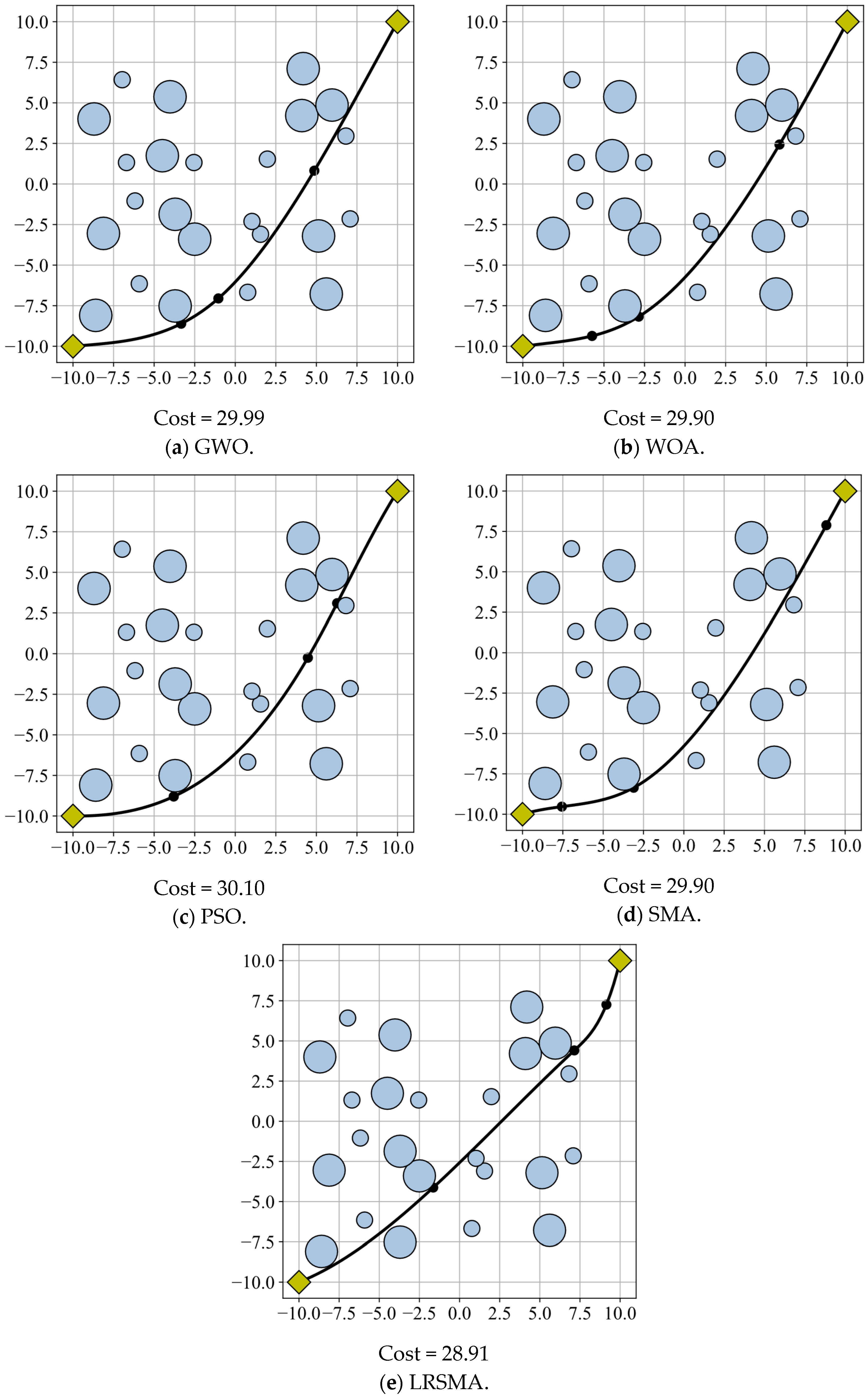
Scenario 3	GWO	30.03	42.52	22.78	2.80	2.81
	WOA	29.90	37.38	93.64	3.11	3.04
	PSO	30.10	37.61	9.46	2.81	2.68
	SMA	29.90	35.82	9.04	2.97	2.94
	LRSMA	28.91	34.58	4.81	2.97	2.98

shows the overall performance of the four algorithms in three scenarios, including the minimum, mean, and standard deviation of the path length for the best solution, the planning time required to obtain the best optimal path, and the mean planning time. Each scenario and algorithm were tested 100 times.

Figure 2, Figure 3 and Figure 4 show the collision-free shortest path results generated by each algorithm, indicating that all algorithms can generate collision-free paths. In these figures, blue circles represent obstacles, with larger radii indicating larger obstacles. Black dots represent the coordinates of path nodes, while yellow diamonds represent the starting and ending points. A comparison of path lengths between the LRSMA and other algorithms is shown in

Table 4. Comparison of the percentage change in the minimum path length for the best solution among the LRSMA and three other algorithms.

	GWO-LRSMA % Change in Minimum	WOA-LRSMA % Change in Minimum	PSO-LRSMA % Change in Minimum	SMA-LRSMA % Change in Minimum
Scenario 1	0.14	−0.03	0.82	−0.03
Scenario 2	0.07	4.59	7.65	7.65
Scenario 3	3.73	3.31	3.95	3.31

and

Table 5. Comparison of the percentage change in the mean path length for the best solution among the LRSMA and three other algorithms.

	GWO-LRSMA % Change in Mean	WOA-LRSMA % Change in Mean	PSO-LRSMA % Change in Mean	SMA-LRSMA % Change in Mean
Scenario 1	1.09	0.37	1.42	0.23
Scenario 2	13.19	3.32	5.80	0.55
Scenario 3	18.67	7.49	8.06	3.46

.

Figure 2a–d shows the best solutions generated by all the algorithms in the first scenario. In the first scenario, the LRSMA had a slight difference in the minimum and mean path length compared to the other algorithms. The PSO has the shortest solving time, followed by the SMA, WOA, GWO, and LRSMA. This is because the LRSMA’s variable neighborhood flight consumes time. In simple scenarios, the LRSMA has little advantage over the other three algorithms. The SMA is less likely to fall into local optimization in simple scenarios, so the LRSMA’s rotation perturbation mechanism has difficulty functioning effectively. The LRSMA’s planning time is greater than that of the SMA due to its need to monitor the population state and perturb it if it is stagnating.

Figure 3a–d shows the best solution generated by all the algorithms in the second scenario. In the second scenario, the LRSMA reduces the minimum of the path length by 0.07% compared with the GWO, 4.59% compared with the WOA, 7.65% compared with the PSO, and 7.65% compared with the SMA. Meanwhile, the LRSMA reduces the mean of the path length by 13.19% compared with the GWO, 3.32% compared with the WOA, 5.80% compared with the PSO, and 0.55% compared with the SMA. Moreover, the LRSMA is better than the GWO, WOA, PSO, and SMA in terms of the standard deviation of the path length. In addition, the planning time of the GWO, SMA, PSO, and LRSMA differs by 0.1 and is less than that of the WOA. There is a difference of 0.2 between the planning time of the best optimal path and the mean planning time for all algorithms. In complex scenarios, the GWO, WOA, PSO, and SMA take longer as the scenario complexity increases. The strategy proposed by LRSMA accelerates the algorithm’s convergence, making the planning times similar across all algorithms. Furthermore, the time consumed by the LRSMA is relatively stable in all scenarios. This indicates that the proposed rotation perturbation mechanism in this paper can improve the algorithm’s global search and local exploitation capabilities, therefore improving the convergence efficiency of the algorithm and finding shorter paths.

Figure 4a–d shows the best solution generated by all the algorithms in the third scenario. In the third scenario, the LRSMA reduces the minimum path length by 3.37% compared with the GWO, 3.31% compared with the WOA, 3.95% compared with the PSO, and 3.31% compared with the SMA. Meanwhile, the LRSMA reduces the mean of the path length by 18.67% compared with the GWO, 7.49% compared with the WOA, 8.06% compared with the PSO, and 3.46% compared with the SMA. Moreover, the standard deviation of path length for the best solution obtained by the LRSMA is 4.81, which is less than those of the GWO, WOA, SMA and PSO. Moreover, the LRSMA and SMA have longer planning times than the GWO and PSO and shorter planning times than WOA. In addition, there is a difference of 0.1 between the planning time of the best optimal path and the mean planning time for all algorithms. In complex scenarios, the GWO, WOA, PSO, and SMA take longer time as the scenario complexity increases. The strategy proposed by LRSMA accelerates the algorithm’s convergence, making the planning times similar across all algorithms. Furthermore, the time consumed by the LRSMA is relatively stable in all scenarios. This is because the Lévy algorithm enhances the global search capability of the algorithm, while the rotation perturbation increases the local development capability of the algorithm. This indicates that the path modification of LRSMA is the most stable, and the rotation perturbation mechanism proposed in this paper can monitor the algorithm state and jump out of local optima, finding a shorter path.

Overall, the LRSMA produces more stable, collision-free, and shorter paths in both simple and complex scenarios compared with the other algorithms, especially in complex scenarios with obstacles on the path from the starting point to the destination.

Figure 5 shows the iteration curves of the four algorithms in the third scenario, revealing that LRSMA convergence requires more iterations than the SMA. GWO stopped at the 26th iteration. The WOA suddenly finds the most optimal solution at 25 iterations. The PSO has difficulty improving its results after 17 iterations, while SMA has difficulty improving after 19 iterations. By contrast, the LRSMA slowly converges from the beginning to the later stages of iteration, indicating that the strategy proposed by the LRSMA can detect local optimal traps and achieve slow convergence.

Figure 6 illustrates the iterative path planning curve obtained using the LRSMA in both the first and second scenario. The LRSMA demonstrates a gradual evolution throughout. Moreover, the convergence times in the first scenario are shorter than those in the second scenario. As per the LRSMA’s definition, it requires time to converge after detecting that the population has entered the local optimum. The convergence then takes place after a sufficient number of iterations. Figure 5 and Figure 6 suggest that 30 iterations can achieve satisfactory performance across all scenarios.

6. Conclusions

This paper proposes a path-planning algorithm using the improved SMA for AMRs, achieving shorter and more stable path solutions. The proposed algorithm addresses the issues of local optima trapping and the lack of an effective escape mechanism in SMA path planning. By introducing an elite learning strategy utilizing variable neighborhood Lévy flight and an individual rotational perturbation and variation mechanism based on tolerance, the proposed algorithm enhances the SMA’s global search and local exploitation capabilities and planning capabilities. The experiments conducted on three different obstacle distributions demonstrate that the collision-free path generated by our algorithm has the shortest length, highest accuracy, and greatest stability. However, the LRSMA does not outperform the WOA, PSO, and SMA in terms of time consumption, especially in optimizing the best position variation. The computational cost must be further improved. Additionally, path planning based on SMA in dynamic environments is also an important research direction. Moreover, the algorithm needs to be tested in multi-robot scenarios.

In terms of real-world applications, this algorithm can be applied to autonomous vehicles or slow-moving robots in situations without no road constraints. For autonomous vehicles, it can be used for mapping specific locations, monitoring, or filming scenes. For robots, it can be used in logistics for sorting delivery routes, guiding underground parking in transportation, and other applications. Since this algorithm requires convergence time, it is suitable for situations that do not require urgent and quick responses. For instance, in rescue missions, faster algorithms are needed.

References

- Cui, P.; Yan, W.; Cui, R.; Yu, J.; Ju, Z. Smooth path planning for robot docking in unknown environment with obstacles. Complex 2018, 2018, 4359036. [Google Scholar] [CrossRef] [Green Version]
- Zhao, M.; Lu, H.; Yang, S.; Guo, Y.; Guo, F. A fast robot path planning algorithm based on bidirectional associative learning. Comput. Ind. Eng. 2021, 155, 107173. [Google Scholar] [CrossRef]
- Patle, B.K.; Babu L, G.; Pandey, A.; Parhi, D.R.K.; Jagadeesh, A. A review: On path planning strategies for navigation of mobile robot. Def. Technol. 2019, 15, 582–606. [Google Scholar] [CrossRef]
- Barraquand, J.; Langlois, B.; Latombe, J.-C. Numerical potential field techniques for robot path planning. In Proceedings of the Fifth International Conference on Advanced Robotics 'Robots in Unstructured Environments, Pisa, Italy, 19–22 June 1991; Volume 1012, pp. 1012–1017. [Google Scholar]
- Hao, K.; Zhao, J.; Yu, K.; Li, C.; Wang, C. Path planning of mobile robots based on a multi-population migration genetic algorithm. Sensors 2020, 20, 5873. [Google Scholar] [CrossRef] [PubMed]
- Mu, Y.; Li, B.; An, D.; Wei, Y. Three-dimensional route planning based on the beetle swarm optimization algorithm. IEEE Access. 2019, 7, 117804–117813. [Google Scholar] [CrossRef]
- Wang, H.J.; Fu, Z.J.; Zhou, J.J.; Fu, M.Y.; Ruan, L. Cooperative collision avoidance for unmanned surface vehicles based on improved genetic algorithm. Ocean Eng. 2021, 222, 25. [Google Scholar] [CrossRef]
- Ajeil, F.H.; Ibraheem, I.K.; Sahib, M.A.; Humaidi, A.J. Multi-objective path planning of an autonomous mobile robot using hybrid PSO-MFB optimization algorithm. Appl. Soft Comput. 2020, 89, 106076. [Google Scholar] [CrossRef] [Green Version]
- Sun, Y.; Wang, H.P. A novel A* method fusing bio-inspired algorithm for mobile robot path planning. Eai Endorsed Trans. S 2022, 9, 12. [Google Scholar] [CrossRef]
- Feng, Y.H.; Deb, S.; Wang, G.G.; Alavi, A.H. Monarch butterfly optimization: A comprehensive review. Expert Syst. Appl. 2021, 168, 11. [Google Scholar] [CrossRef]
- Dai, Y.; Yu, J.; Zhang, C.; Zhan, B.; Zheng, X. A novel whale optimization algorithm of path planning strategy for mobile robots. Appl. Intell. 2022. [Google Scholar] [CrossRef]
- Luo, J.; Liu, Z.W. Novel grey wolf optimization based on modified differential evolution for numerical function optimization. Appl. Intell. 2020, 50, 468–486. [Google Scholar] [CrossRef]
- Zhang, L.; Zhang, Y.J.; Li, Y.F. Mobile robot path planning based on improved localized particle swarm optimization. IEEE Sens. J. 2021, 21, 6962–6972. [Google Scholar] [CrossRef]
- Zhang, Y.; Gong, D.-W.; Zhang, J.-H. Robot path planning in uncertain environment using multi-objective particle swarm optimization. Neurocomputing 2013, 103, 172–185. [Google Scholar] [CrossRef]
- Wu, L.; Huang, X.D.; Cui, J.G.; Liu, C.; Xiao, W.S. Modified adaptive ant colony optimization algorithm and its application for solving path planning of mobile robot. Expert Syst. Appl. 2023, 215, 22. [Google Scholar] [CrossRef]
- Liu, C.; Wu, L.; Huang, X.D.; Xiao, W.S. Improved dynamic adaptive ant colony optimization algorithm to solve pipe routing design. Knowledge-Based Syst. 2022, 237, 13. [Google Scholar] [CrossRef]
- Nakagaki, T.; Yamada, H.; Ueda, T. Interaction between cell shape and contraction pattern in the physarum plasmodium. Biophys. Chem. 2000, 84, 195–204. [Google Scholar] [CrossRef]
- Cai, Z.; Xiong, Z.; Wan, K.; Xu, Y.; Xu, F. A node selecting approach for traffic network based on artificial slime mold. IEEE Access. 2020, 8, 8436–8448. [Google Scholar] [CrossRef]
- Hassan, M.H.; Kamel, S.; Abualigah, L.; Eid, A. Development and application of slime mould algorithm for optimal economic emission dispatch. Expert Syst. Appl. 2021, 182, 28. [Google Scholar] [CrossRef]
- Agarwal, D.; Bharti, P.S. Implementing modified swarm intelligence algorithm based on slime moulds for path planning and obstacle avoidance problem in mobile robots. Appl. Soft Comput. 2021, 107, 107372. [Google Scholar] [CrossRef]
- Naik, M.K.; Panda, R.; Abraham, A. An entropy minimization based multilevel colour thresholding technique for analysis of breast thermograms using equilibrium slime mould algorithm. Appl. Soft Comput. 2021, 113, 107955. [Google Scholar] [CrossRef]
- Abdel-Basset, M.; Mohamed, R.; Chakrabortty, R.K.; Ryan, M.J.; Mirjalili, S. An efficient binary slime mould algorithm integrated with a novel attacking-feeding strategy for feature selection. Comput. Ind. Eng. 2021, 153, 107078. [Google Scholar] [CrossRef]
- Li, S.; Chen, H.; Wang, M.; Heidari, A.A.; Mirjalili, S. Slime mould algorithm: A new method for stochastic optimization. Future Gener. Comput. Syst. 2020, 111, 300–323. [Google Scholar] [CrossRef]
- Dai, X.; Long, S.; Zhang, Z.; Gong, D. Mobile robot path planning based on ant colony algorithm with A* heuristic method. Front. Neurorob. 2019, 13. [Google Scholar] [CrossRef] [PubMed] [Green Version]
- Szczepanski, R.; Bereit, A.; Tarczewski, T. Efficient local path planning algorithm using artificial potential field supported by augmented reality. Energies 2021, 14, 6642. [Google Scholar] [CrossRef]
- Qi, J.; Yang, H.; Sun, H. Mod-RRT*: A sampling-based algorithm for robot path planning in dynamic environment. IEEE Trans. Ind. Electron. 2021, 68, 7244–7251. [Google Scholar] [CrossRef]
- Chang, Y.-C.; Shi, Y.; Dostovalova, A.; Cao, Z.; Kim, J.; Gibbons, D.; Lin, C.-T. Interpretable fuzzy logic control for multirobot coordination in a cluttered environment. IEEE Trans. Fuzzy Syst. 2021, 29, 3676–3685. [Google Scholar] [CrossRef]
- Qu, H.; Yang, S.X.; Willms, A.R.; Yi, Z. Real-time robot path planning based on a modified pulse-coupled neural network model. IEEE Trans. Neural Netw. 2009, 20, 1724–1739. [Google Scholar] [CrossRef]
- Nazarahari, M.; Khanmirza, E.; Doostie, S. Multi-objective multi-robot path planning in continuous environment using an enhanced genetic algorithm. Expert Syst. Appl. 2019, 115, 106–120. [Google Scholar] [CrossRef]
- Zhao, Z.; Jin, M.; Lu, E.; Yang, S.X. Path planning of arbitrary shaped mobile robots with safety consideration. IEEE Trans. Intell. Transp. Syst. 2022, 23, 16474–16483. [Google Scholar] [CrossRef]
- Cui, Y.; Hu, W.; Rahmani, A. A reinforcement learning based artificial bee colony algorithm with application in robot path planning. Expert Syst. Appl. 2022, 203, 117389. [Google Scholar] [CrossRef]
- Das, P.K.; Jena, P.K. Multi-robot path planning using improved particle swarm optimization algorithm through novel evolutionary operators. Appl. Soft Comput. 2020, 92, 106312. [Google Scholar] [CrossRef]
- Wang, L.; Kan, J.; Guo, J.; Wang, C. 3D path planning for the ground robot with improved ant colony optimization. Sensors 2019, 19, 815. [Google Scholar] [CrossRef] [PubMed] [Green Version]
- Teng, Z.-j.; Lv, J.-l.; Guo, L.-w. An improved hybrid grey wolf optimization algorithm. Soft Comput. 2019, 23, 6617–6631. [Google Scholar] [CrossRef]
- Fernandes, P.B.; Oliveira, R.C.L.; Fonseca Neto, J.V. Trajectory planning of autonomous mobile robots applying a particle swarm optimization algorithm with peaks of diversity. Appl. Soft Comput. 2022, 116, 108108. [Google Scholar] [CrossRef]
- Yu, C.; Heidari, A.A.; Xue, X.; Zhang, L.; Chen, H.; Chen, W. Boosting quantum rotation gate embedded slime mould algorithm. Expert Syst. Appl. 2021, 181, 115082. [Google Scholar] [CrossRef]
- Nguyen, T.-T.; Wang, H.-J.; Dao, T.-K.; Pan, J.-S.; Liu, J.-H.; Weng, S. An improved slime mold algorithm and its application for optimal operation of cascade hydropower stations. IEEE Access. 2020, 8, 226754–226772. [Google Scholar] [CrossRef]
- Rizk-Allah, R.M.; Hassanien, A.E.; Song, D. Chaos-opposition-enhanced slime mould algorithm for minimizing the cost of energy for the wind turbines on high-altitude sites. ISA Trans. 2022, 121, 191–205. [Google Scholar] [CrossRef]
- Houssein, E.H.; Helmy, B.E.-d.; Rezk, H.; Nassef, A.M. An efficient orthogonal opposition-based learning slime mould algorithm for maximum power point tracking. Neural Comput. Appl. 2022, 34, 3671–3695. [Google Scholar] [CrossRef]
- Houssein, E.H.; Mahdy, M.A.; Blondin, M.J.; Shebl, D.; Mohamed, W.M. Hybrid slime mould algorithm with adaptive guided differential evolution algorithm for combinatorial and global optimization problems. Expert Syst. Appl. 2021, 174, 114689. [Google Scholar] [CrossRef]
- Liu, Y.; Liu, S. Unscented sigma point guided quasi-opposite slime mould algorithm and its application in engineering problem. Appl. Res. Comput. 2022, 39, 2709–2716. [Google Scholar] [CrossRef]
- Wang, J.; Elia, N. Distributed averaging under constraints on information exchange: Emergence of lévy flights. IEEE Trans. Automat. Contr. 2012, 57, 2435–2449. [Google Scholar] [CrossRef]
- Mantegna, R.N. Fast, accurate algorithm for numerical simulation of lévy stable stochastic processes. Phys. Rev. E 1994, 49, 4677–4683. [Google Scholar] [CrossRef] [PubMed]
- Hwang, C.-R. Simulated annealing: Theory and applications. Acta Appl. Math. 1988, 12, 108–111. [Google Scholar] [CrossRef]
- Lian, J.; Yu, W.; Xiao, K.; Liu, W. Cubic spline interpolation-based robot path planning using a chaotic adaptive particle swarm optimization algorithm. Math. Probl. Eng. 2020, 2020, 1–20. [Google Scholar] [CrossRef]
- Sang-To, T.; Le-Minh, H.; Mirjalili, S.; Wahab, M.A.; Cuong-Le, T. A new movement strategy of grey wolf optimizer for optimization problems and structural damage identification. Adv. Eng. Softw. 2022, 173, 31. [Google Scholar] [CrossRef]
- Mirjalili, S.; Lewis, A. The whale optimization algorithm. Adv. Eng. Softw. 2016, 95, 51–67. [Google Scholar] [CrossRef]