Review

Change Detection Applications in the Earth Sciences Using UAS-Based Sensing: A Review and Future Opportunities

by
Christian G. Andresen
1,* and
Emily S. Schultz-Fellenz
2
1
Geography Department, University of Wisconsin Madison, Madison, WI 53706, USA
2
Earth and Environmental Sciences Division, Los Alamos National Laboratory, Los Alamos, NM 87545, USA
*
Author to whom correspondence should be addressed.
Drones 2023, 7(4), 258; https://doi.org/10.3390/drones7040258
Submission received: 24 February 2023 / Revised: 3 April 2023 / Accepted: 5 April 2023 / Published: 11 April 2023

Abstract

:
Over the past decade, advancements in collection platforms such as unoccupied aerial systems (UAS), survey-grade GNSS, sensor packages, processing software, and spatial analytical tools have facilitated change detection analyses at an unprecedented resolution over broader spatial and temporal extents and in environments where such investigations present challenges. These technological improvements, coupled with the accessibility and versatility of UAS technology, have pushed the boundaries of spatial and temporal scales in geomorphic change detection. As a result, the cm-scale analysis of topographic signatures can detect and quantify surface anomalies during geomorphic evolution. This review focuses on the use of UAS photogrammetry for fine spatial (cm) and temporal (hours to days) scale geomorphic analyses, and it highlights analytical approaches to detect and quantify surface processes that were previously elusive. The review provides insight into topographic change characterization with precise spatial validations applied to landscape processes in various fields, such as the cryosphere and geosphere, as well as anthropogenic earth processes and national security applications. This work sheds light on previously unexplored aspects of both natural and human-engineered environments, demonstrating the potential of UAS observations in change detection. Our discussion examines the emerging horizons of UAS-based change detection, including machine learning and LIDAR systems. In addition, our meta-analysis of spatial and temporal UAS-based observations highlights the new fine-scale niche of UAS-photogrammetry. This scale advancement sets a new frontier in change detection, offering exciting possibilities for the future of land surface analysis and environmental monitoring in the field of Earth Science.

1. Introduction

Remote change detection has been a key component for understanding Earth surface dynamics and associated environmental processes from local to global scales [1]. Surface dynamics are tightly coupled with the transport of mass and energy, which are critical factors that allow us to better understand and predict biophysical feedbacks and landscape evolution [2]. The ability to quantify landscape change detection is generally based on quantifying spatiotemporal differences of surfaces based on spectra or elevation to capture signatures of change. In particular, the detection of geomorphic change, relating to Earth’s surface processes, has relied on the comparison of digital surface models (DSMs) or 3D point clouds to estimate and model surface changes that can be translated to elevation and volume. Spaceborne and crewed aircraft-based remote sensing have been the standard for detection, quantification, and understanding of morphological changes and dynamics of geological processes, including glaciers, landslides, coastal change, and earthquakes (e.g., [1,3,4]). In general, geomorphic processes have been characterized infrequently at long time scales (i.e., months to years) from space and airplane platforms with moderate to coarse spatial resolution. This coarse spatial and temporal resolution may overlook key processes occurring at smaller scales and faster phases. The acquisition and analysis of fine-scale data through ground-based or surface-proximal methods allow improved constraint and understanding of the mechanisms responsible for the broad-scale surface signatures detected by higher-altitude remote sensing platforms. Therefore, the advancement of technologies for fine-scale change detection has been critical in geosciences.
Over the past two decades, change detection at fine scales has been mostly led by Terrestrial Laser Scanning (TLS) approaches, allowing mm- to cm-scale observations over a diverse range of surface processes [5,6,7]. The high resolution and accuracy of this system has made it a reliable tool that has advanced multiple fields including structural geology, seismology, natural hazards, geomorphology, and glaciology. However, its cost, intrusive deployment configurations, short range, and burdensome lack of portability (especially in remote locations) makes TLS a challenging option for change detection analysis. With the emergence of photogrammetric approaches added to advances in the use of unoccupied aerial systems (UAS) at a fraction of the cost of TLS, UAS has gained popularity as a cost-effective, versatile, and relatively accurate tool for change detection. Within this review, we define UAS as an integrated aerial system consisting of a small uncrewed aircraft and at least one onboard sensor. This pairing of the aircraft and sensor creates a complete and functional system capable of aerial data collection and analysis for various applications.
The ability to derive detailed topographic changes at fine spatial scales through UAS photogrammetric approaches has opened a new era for surface characterization of the Earth. Recent and growing technological advancements in UAS combined with cutting-edge computer vision-based digital photogrammetry, commonly known as Structure-from-Motion (SfM) [8,9], has revolutionized our understanding of and our ability to quantify surface geomorphic signatures compared to commonly used approaches, such as spaceborne, airplane-based, and ground-based approaches. In particular, UAS SfM versatility due to cost-effective sampling at high temporal and spatial scales has made topographic assessments more accessible to geoscientists, enhancing the field of detection of surface signatures and geomorphic change.
The popularity of UAS-based change detection across the Earth sciences is reflected in the sharp increase in the number of publications relying on UAS over the past decade [10,11,12]. In addition, worldwide accessibility of UAS technology which retails at a fraction of the cost compared to Light Detection and Ranging (LIDAR) technology, has boosted its use in the Earth sciences for quantification of processes at high temporal and spatial scales. The feasibility and ease of capturing multiple observations over hourly to daily scales has filled a niche in observational geosciences and has made this tool very useful for assessing geomorphic evolution and change by comparing the chronosequence of observations [13,14]. This niche, combined with the reduction of risk in traditional field data collections and the increased reliability and flexibility of UAS, will continue to be a common tool for change detection characterization of small surface signatures.
UAS-based change detection applied to the Earth sciences spans a wide array of applications and permits exploration into geomorphic signature formation mechanics and dynamics, which can facilitate expanded applications in areas such as economic geology and related industries [11,15,16]. There have been a number of reviews in recent years of UAS applications in Earth sciences [7,10,12,17,18] as well as change detection methods [1,19,20]. However, a detailed review of the capabilities of UAS-based change detection at fine spatial and temporal scales applied to Earth sciences and processes has not been presented elsewhere. Based on the increasing applications of UAS technologies for change detection, there is an imperative need for a current overview of advancements and applications. Therefore, this paper intends to provide a detailed record on change detection studies that employ fine temporal and spatial scale datasets of surface dynamics in the field of earth sciences, including both natural and anthropogenic Earth processes. This manuscript also intends to showcase trans-disciplinary methodological advances and innovative approaches in process-specific disciplines to expand the frontiers of change detection in the Earth sciences and highlight the emergent horizons in big-data analytics, data fusion, and sensor advancements and uncertainty management.

2. UAS-Based Change Detection Applications

Remote change detection or “the process of identifying differences in the state of an object or phenomenon by observing it at different times” [21] has become a key approach for understanding earth system dynamics. This study focuses on UAS photogrammetry change detection studies that characterize changes in position (2D), elevation (2.5D), and volume (3D) in the Earth sciences and employ a range of change detection algorithms, which are highlighted in Table 1 and Figure 1, and which are discussed and compared in detail by others (i.e., [1,19,20]).

2.1. Applications in Geomorphic Change Detection

2.1.1. Cryosphere

The cryosphere is experiencing significant changes in response to climate change and represents an emergent horizon for the use of UAS in observing and quantifying spatiotemporal changes in these rapidly changing systems [46]. Most notably, permafrost, glaciers, ice sheets, and sea ice enjoy growing scientific attention for change detection, analysis, and monitoring given their vulnerability to polar temperature amplification [47,48]. Most cryospheric change detection studies have utilized spaceborne data, given the remoteness of these landscapes and logistical challenges for in situ monitoring. High latitude observations have been historically limited to relatively coarse spatial and temporal scales as a result of dominant cloud coverage [49]. Furthermore, satellite constellations offer poor polar coverage, and weather difficulties make crewed aircraft-based activities high risk in these regions. Nonetheless, large-scale airborne campaigns have been undertaken in recent years, employing both passive (i.e., hyperspectral, photogrammetric) and active sensors (LIDAR, synthetic aperture radar [SAR]) to characterize and monitor climate change in high latitudes (e.g., NASA ABoVE; see [50]).
Fine-scale change detection of glacial and periglacial landscapes have been generally assessed through TLS at cm-scale [34,51]. However, emerging UAS technologies allow cryosphere studies to employ photogrammetry SfM methods and derive high spatial resolution topographic data comparable to TLS but with high temporal frequency [13,48,52], even continuous temporal monitoring and tracking [53]. Although cryospheric applications employing UAS-based change detection are broad, they concentrate in four main areas (by decreasing order): glacier, snow, landforms, and vegetation [46]. Here, we focus on cryospheric geomorphic change detection studies that focus on 3 key areas: (1) glacier, (2) snow, and (3) landforms.
Glacier studies employing UAS for change detection include quantification and timing of ablation [42,54,55], calving events [41,48,56], flow velocity [13,57], plume dynamics [13], and periglacial processes [58,59,60]. Notably, Jouvet et al. [13] employed a fixed-wing UAS to monitor intra-day (12 h interval) glacier velocity and proglacial plumes over a 12-day period in a tide-water glacier. The study revealed speed-up events (up to 170%) within 48 h of enhanced acceleration as well as the evolution of flow plumes with pulsating water jets (Figure 2). Furthermore, Adams et al. [52] characterized hourly glacier calving dynamics and observed sudden rapid deformation prior to calving (Figure 3).
The presence of snow during its seasonal coverage significantly affects various environmental factors, such as albedo, vegetation, and soil properties, including soil thermal dynamics, which are critical components of the Earth’s surface energy balance. In addition, snow quantification represents a key factor for forecasting potential hazards such as avalanches and flooding. Characterization of snow cover is fairly routine, but quantification of snow depth has been challenging and positively accomplished through change detection [61,62]. However, cm-scale snow depth measurements provide a new insight into the heterogeneity of snow distribution and, most importantly, the evolution and melt of snow over high temporal frequency. Eker et al. [14] employed UAS daily observations at cm-scale to track ablation dynamics at microscales, thus detecting “hot-spots”, areas with higher rates of snow melt, which shows how landscape properties and processes influence snow depth over fine spatial and temporal scales. Similarly, Bernard et al. [63] employed UAS seasonal surveys to characterize snow accumulation, icing, and melting dynamics. It should be noted that fine-scale observations of snow depth assume a stable ground surface under snow and soil cryogenic processes, such as ground heaving, permafrost creep, etc., can contribute to errors in the snow depth computation [64].
Permafrost landforms and processes have been investigated with UAS-based photogrammetry at high spatial and temporal resolutions. For example, seasonal monitoring of poorly drained areas in continuous permafrost showed significant uplift and settlement of up to 50 cm as a result of ice lens development and thaw in saturated soils adjacent to infrastructure [65] (Figure 4). Seasonal observations of organic peatlands revealed the development of frost boils during summer time [66]. Tracking of permafrost thaw slumps showed seasonal complexities of thaw slump development and spatial distribution at daily to decadal scales showing increases of sediment export [65].
Other examples of UAS-based change detection in the cryosphere: Li et al. [47] employedphotogrammetry methods for monitoring Antarctic sea ice without requiring the coordinated deployment of dense ground control. This innovative work has the potential to open a new frontier in high latitude ice monitoring. Similarly, UAS-based SfM has enabled unique observations on surface changes and sublimation rates in perennially frozen Antarctic lakes, as demonstrated by Ponti et al. [67]. Additionally, UAS-based photogrammetry has been employed in the study of periglacial features in Antarctica, such as solifluction landforms, coastal landforms, and patterned ground, and how it is being influenced by climate change. This approach has been shown to improve spatial analyses of these features, and has identified important periglacial features that were missed by satellite- and crewed aircraft-captured imagery, as found by [68].

2.1.2. Structural Geology and Active Fault Characterization
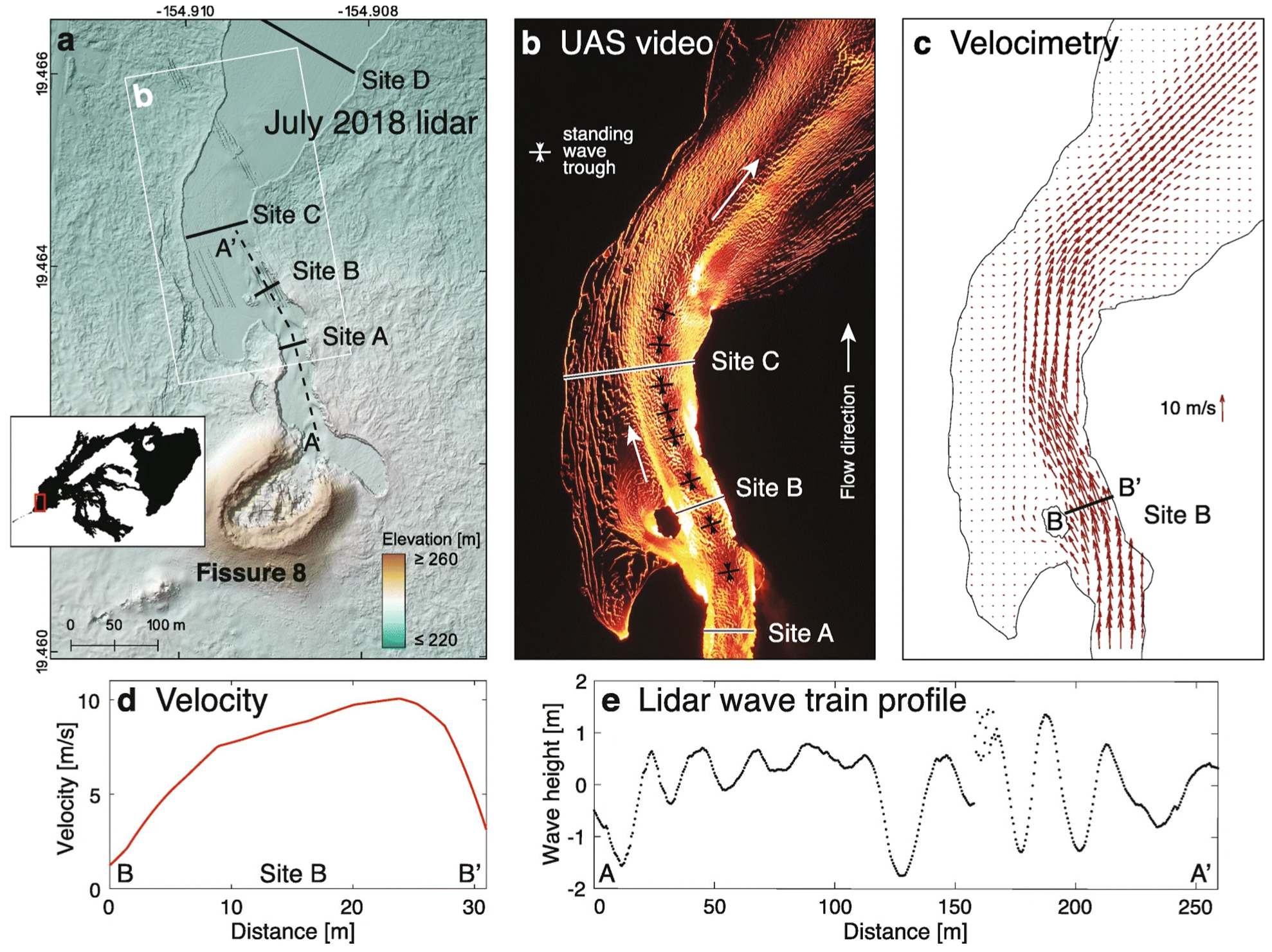
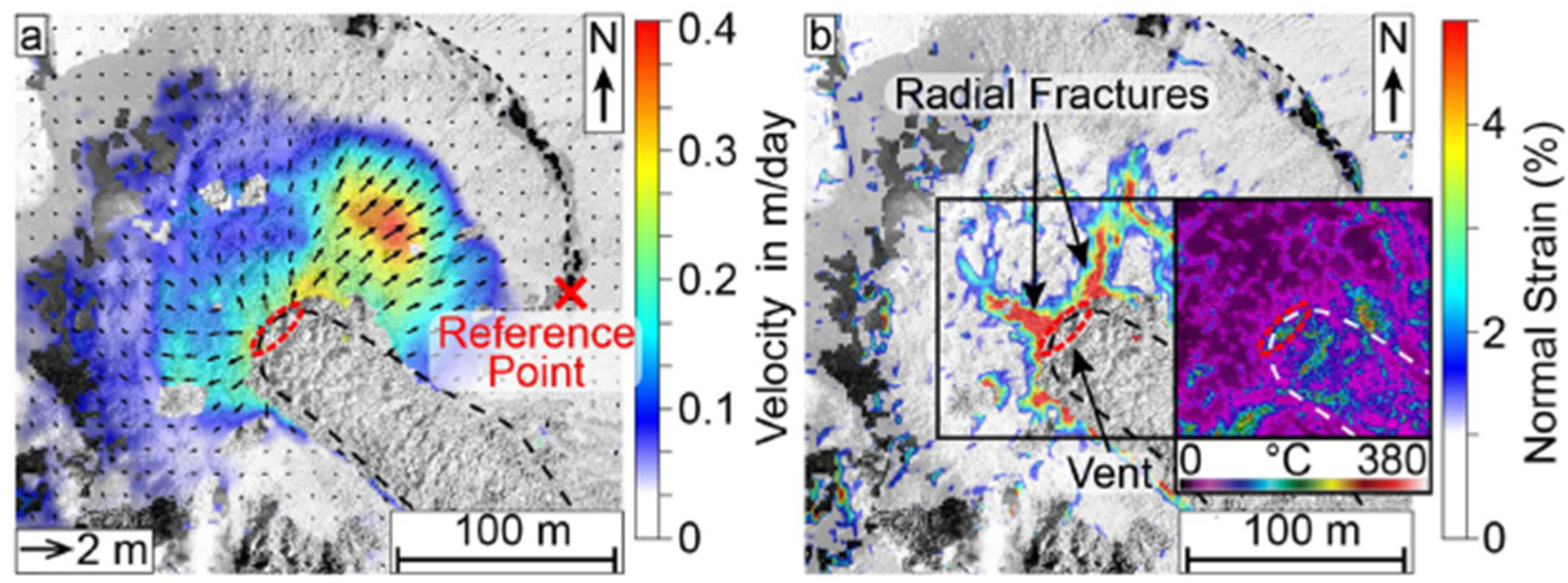
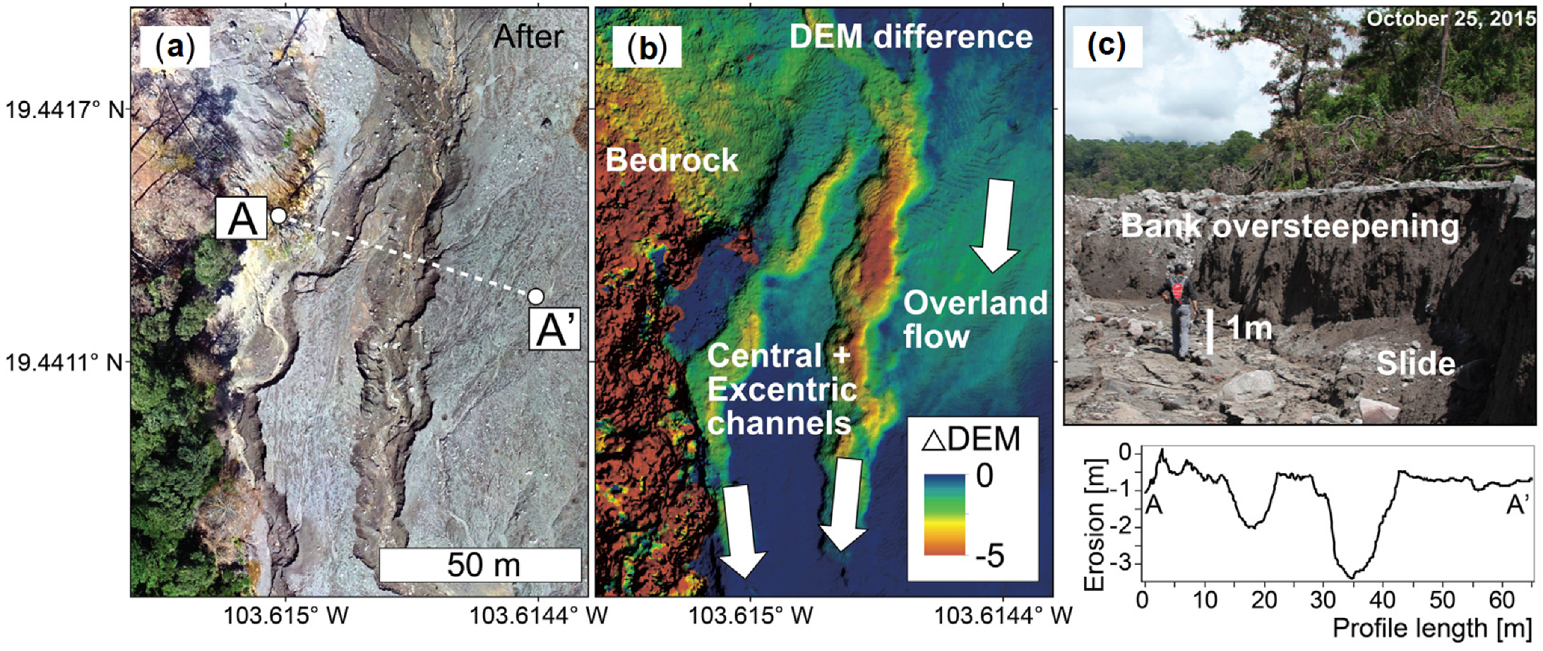
Observation and quantification of faulted landscapes and slip rate analysis have been major components for understanding the influences of tectonic processes on Earth surface dynamics, but human-collected measurements over large areas are expensive and high-risk. Satellite and crewed aircraft-based LIDAR at sub-meter spatial scale have been used for detection and monitoring of faults [69], and they have often been complemented by localized cm-scale differential GPS field surveys and TLS [70]. With modern satellite assets such as WorldView-2 satellite imagery, stereo pair satellite-derived DEM spatial resolution is high (i.e., 5 m), and in some cases up to 0.5 m. The cm-scale spatial-resolution of topographic data derived by UAS photogrammetric approaches enables the constraint of higher-accuracy spatial characteristics of fault activity, which in turn permits estimation of surface dynamics and fault slip rates compared to satellite and airplane LIDAR topographic data [71,72]. In recent years, UAS-based photogrammetry has become more prevalent in the fields of fault characterization, slip rate, and tectonic deformation due to its high spatial resolution and ability to capture detailed observations. However, while UAS photogrammetry has been useful for detecting changes over short periods of time, multi-temporal change detection approaches have utilized a combination of UAS photogrammetry with other topographic datasets such as Terrestrial Laser Scanning (TLS) and spaceborne data (as described by Török et al. [73]), plus historical aerial photogrammetry, which enables researchers to expand the temporal window of analysis.

2.1.3. Volcanology

High spatial and temporal frequency monitoring of volcanic processes with UAS is revolutionizing volcanology [74]. The nature of most volcanic processes makes UAS a great option, since ground-based data collection is generally limited and extremely high-risk. Geomorphic change associated with episodic events such as volcanic eruptions [75], lava flows [76,77], and faulting and ground deformation [37] has been assessed with UAS. Nakano et al. [75] employed a long-range fixed wing UAS to map active volcanic island emergence and expansion, and calculated a 28-fold increase in the island volume after eruption. High-resolution morphological changes of lava flow and fracture mapping are providing novel insights into volcanic structural evolution and potential hazards [37,76]. High frequency temporal monitoring employing particle image velocity on UAS-collected time-series images has allowed calculation of lava flow velocities, volume, and time-averaged discharge rates during eruption [77] (Figure 5), deformation of a lava dome expansion with estimates of normal and shear stress [78] (Figure 6), and quantification of caldera growth, eruption volume, and determination of possible flow pathways using the UAS-derived detailed topography [77]. Walter et al. [79] used UAS to monitor morphological changes, which, in turn, allowed rapid interpretations on eruption locations, timing, and dynamics. James et al. [74] highlight a gamut of other UAS applications in volcanology, including soil, water, and gas sampling from craters as well as gravity and thermal properties of volcanic processes.

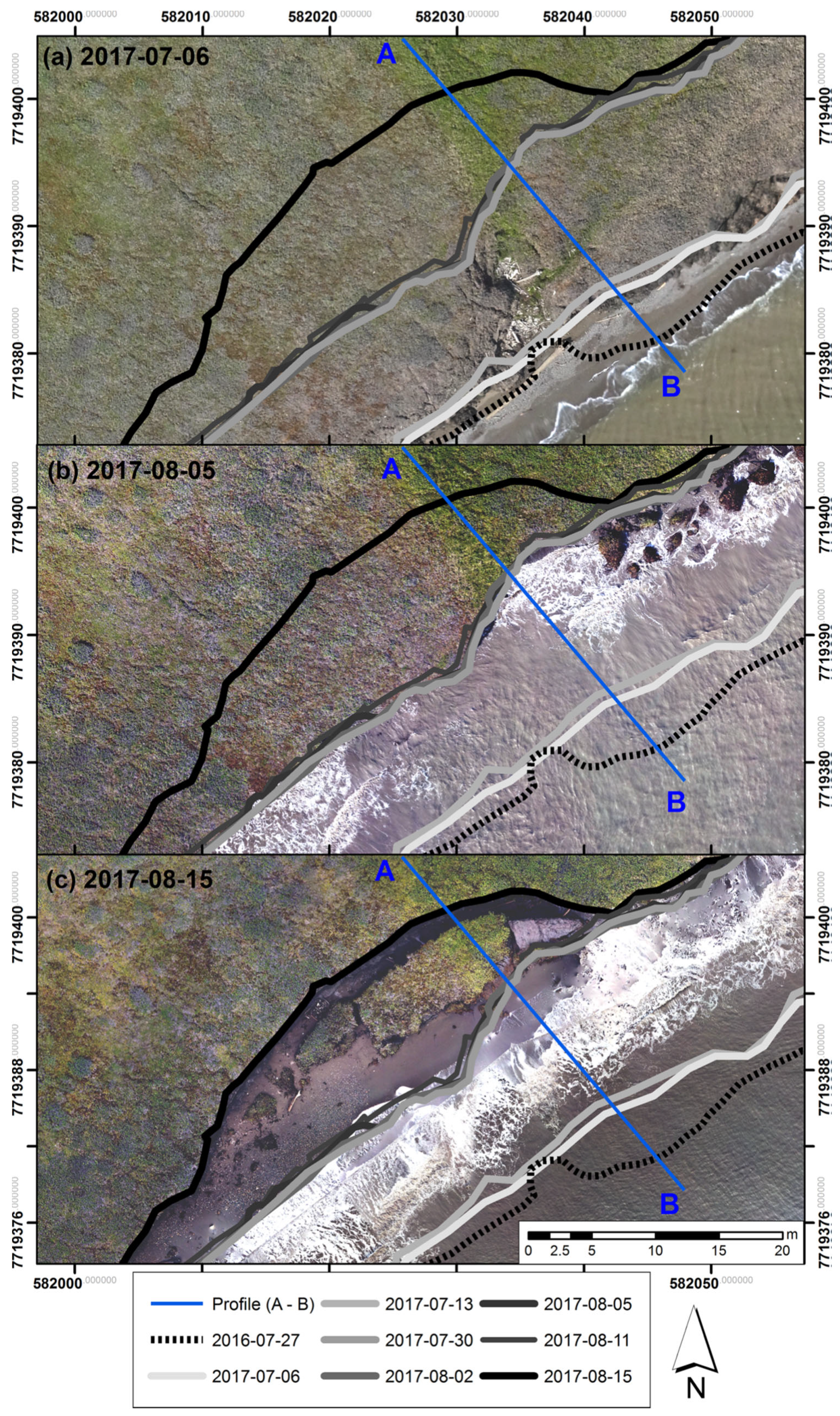
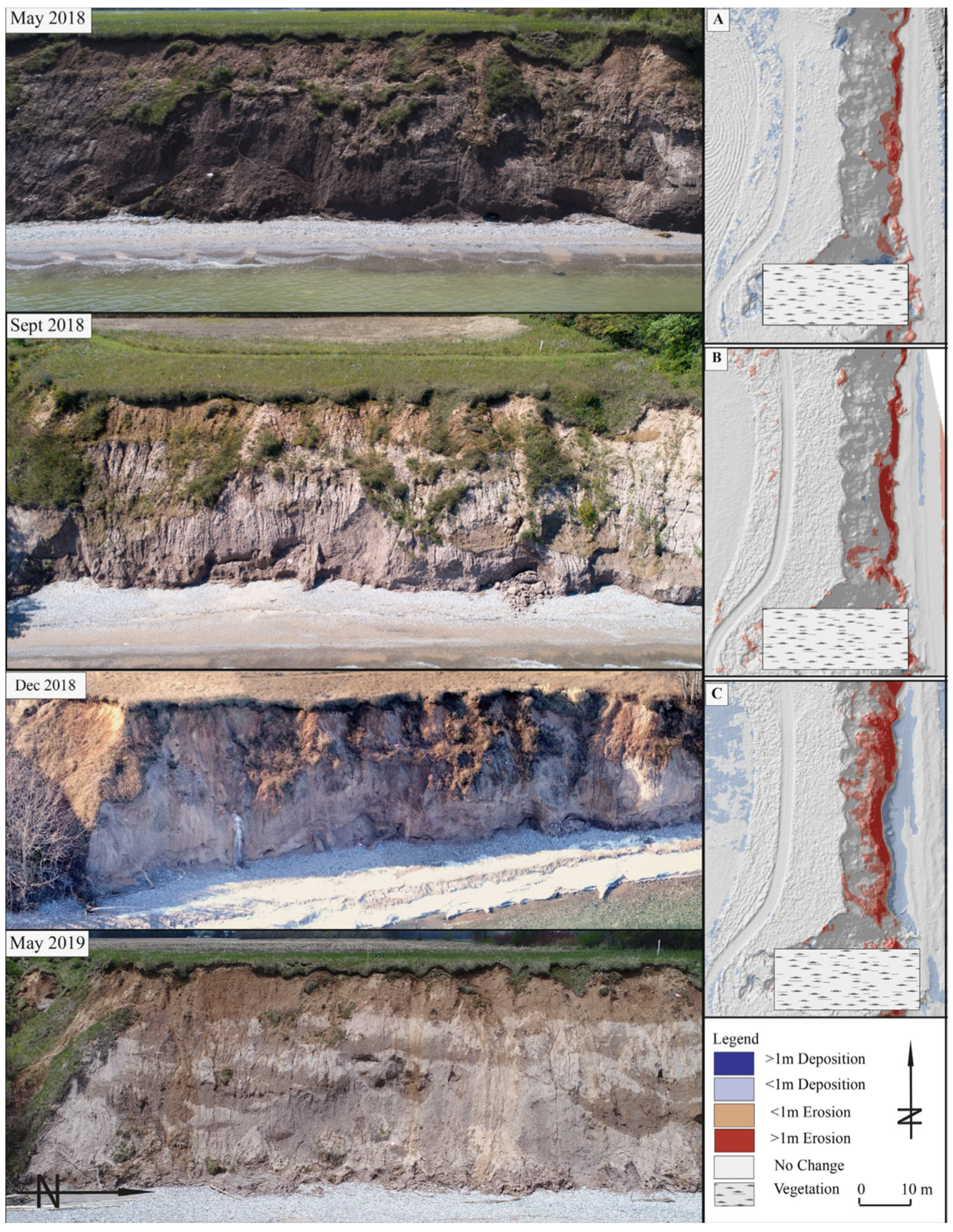
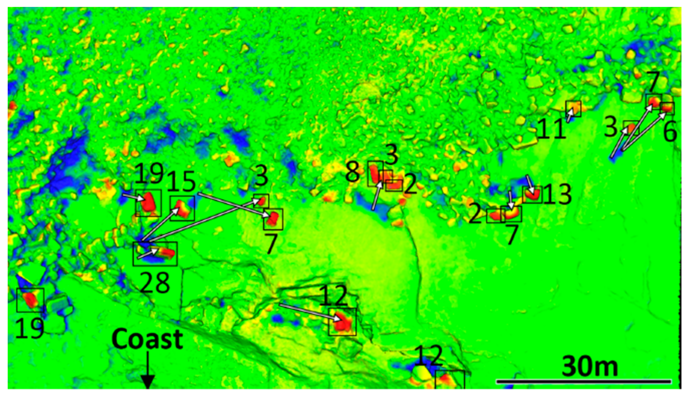
2.1.4. Coastal Geomorphology

With focus on coastal landforms (i.e., beaches, cliffs, shorefaces, etc.), the highly-dynamic coastal geomorphology mobilizes large amounts of sediment and organic matter. Therefore, in this topical area even cm-scale surface changes can translate to megatons of sediment export and/or import. This field has received greater attention given the vulnerability of the terrestrial-aquatic interfaces to climate change through hydrological cycle intensification (i.e., strengthening of storms), sea level rise [10,80], and the juncture of coastal erosion and the impact on anthropogenic infrastructure [81]. These fields have relied on high resolution satellite and airborne imagery as well as LIDAR products to estimate long-term dynamics. The accelerated increases in coastal and river bank dynamics [24,82] methods used to study these systems must increase both the temporal (i.e., hours, days) and spatial scale of surface characterization to allow for quantification of surface changes and identification of physical drivers. Most weather events such as storms, floods, etc. have a time span of hours, and monitoring systems that can cope with this demanding temporal scale are therefore key to improving understanding of the geomorphic evolution as it is impacted by the system [10]. Recent coastal mass wasting studies have assessed short-term intra-seasonal changes to pinpoint environmental controls of erosion rates. For example, Cunliffe et al. [82] recorded erosion rates of 14.5 m/year, six times the historical rate observed over a 70-year record.
By measuring bluff slumping on a weekly basis, researchers can capture short-term changes in the shoreline that may not be apparent at longer time scales. Additionally, analyzing the influence of storm events on shoreline change can provide insights into the role of extreme weather events in shaping coastal landscapes (Figure 7). Similarly, monitoring studies employing UAS SfM surface models of coastal dunes and seasonal slumping rates of lake shore bluffs highlight the importance of quantifying short-term sediment volume changes and erosion timing for managing coastal areas [23,24,80] (Figure 8). Overall, this research approach can contribute to the development of effective coastal management and adaptation strategies by enhancing our understanding of the underlying causes and patterns of shoreline change. UAS represents a practical and affordable solution for detecting the timing and intensity of both abrupt and gradual erosion processes, including the intra-seasonal erosion and accretion patterns that shape coastal landscapes.

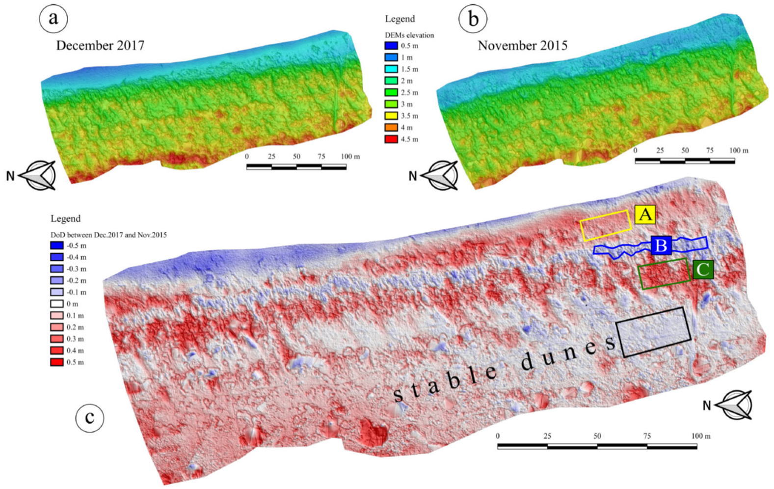
2.1.5. Aeolian Geomorphology

The patterns of dunes are closely linked to weather conditions such as wind and rainfall, making them a sensitive indicator of climate dynamics. This connection between dune formation and weather patterns applies not only to terrestrial landscapes but also to other planets, where dune fields can provide valuable insights into planetary weather conditions [83]. Therefore, the morphological characterization and dynamics of these systems at fine spatial scales is of key importance. Studies focusing on dune systems have emphasized the reliability and efficacy of UAS as a low-cost solution over satellite and LIDAR for capturing fine spatial-scale surface dynamics in dunes [84,85] (Figure 9). UAS high-temporal resolution include interannual monitoring of coastal dune systems’ progradation and erosion [80,86], development of embryo dunes [87], dune stabilization by vegetation [88], intertidal dune dynamics [89] monitoring of storm event impacts [90], and dune migration [91]. The fragility of these landscapes and the encroachment of humans into dune regions makes high-spatiotemporal characterization of dune features an important horizon for ecosystem management and regional conservation policies (e.g., [92,93]).

2.1.6. Fluvial Geomorphology
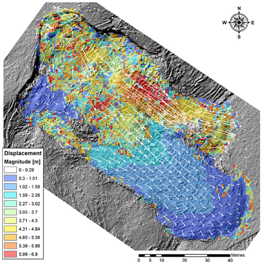
Fluvial geomorphology has benefited from the increases in both temporal and spatial resolutions provided by UAS photogrammetry. High spatial resolution (<20 cm) continuous seasonal monitoring of channel deposition and erosion through low-cost UAS photogrammetry techniques can better inform decision makers, particularly for waterways sensitive to flooding and those that are morphologically dynamic [94,95,96]. In addition, deployment flexibility with UAS has enabled the capture of transient geomorphic changes associated with weather events (i.e., storms, hurricanes) that occur on only a few days per year, such as flash floods and debris flows that can drastically alter sediment redistribution [36,97] (Figure 10). Studies lacking pre-event datasets have modeled the initial topography to perform change detection in fluvial geomorphology. For example, Ellet et al. [98] characterized post-wildfire stream channel erosion without a pre-event dataset by comparing post-event channel characterization with a synthetic DEM that simulates pre-event conditions by delineating and removing channel scoured points from post-event SfM pointcloud and fitting an interpolated surface to simulate pre-event conditions.

2.1.7. Mass Wasting

Mass wasting events include landslides, rockfalls, debris flow, mudflows, soil and rock avalanches, and soil deformational creep. The ability to detect, quantify, and monitor mass wasting enables analytical advancements in geomorphology and hazard management, especially within the built environment. Generally, mass wasting events occur on the scale of meters to kilometers and vary largely on the temporal scale from hours to decades. Thus, these processes can be captured well with the cm sensitivity of UAS, particularly in hazardous and remote locations [45,99,100]. Most mass wasting change detection studies have focused on landslides. For example, Lucieer et al. [40] tested UAS-enabled SfM to quantify terrain displacement dynamics from a landslide over seasonal scales (Figure 11). Employing fine-scale UAS surveys, Saito et al. [100] also identify 54 coseismic landslides within a 1 km2 study area, with volumes ranging from 9.1 to 3994.6 m3. Kyriou et al. [101] used UAS SfM to monitor a slow, active landslide in Greece, and facilitated novel analyses on the role that lithology plays in landslide occurrence and how temporal dynamics can affect swelling clays, which may contribute to active landslide behavior. The temporal yield of mass wasting events can help improve quantification of sediment transport and better constrain its effects on fluvial landforms [99]. Boulder deposits and dynamics have also been assessed using UAS-deployed sensors. Nagle-McNaughton and Cox et al. [33] detected and traced boulder movement documenting movement of boulders and the stochastic nature of boulder transport, where some experience movement while adjacent boulders of the same size are unaffected (Figure 12). Other studies have focused on the quantification of coastal cliff recession to estimate monthly rockfall inventory and identify possible trends in the factor of safety calculations that may be able to predict failure locations [102].

2.2. Applications in Anthropogenic Earth Processes

Anthropogenic activities have been an expanding driver of geomorphic landscape changes, including surface hydrologic alterations, exacerbating and/or restricting erosion, creating ground subsidence, and initiating mass wasting events. Change detection employing UAS has been an emergent tool for economic geology and national security applications. Below, we discuss case studies on economic geology, ground water monitoring, explosion monitoring, and border security.

2.2.1. Economic Geology

Characterization of aboveground mining activities and regions has traditionally relied on airborne and TLS LIDAR systems, which require increasing costs to deploy at a higher risk to personnel. The affordability and high-resolution of photogrammetric data collected from UAS compared to LIDAR systems has made SfM a cost-effective option for industry, particularly by enabling high temporal monitoring of these sites [103]. Both underground and aboveground mining activities increasingly employ UAS and SfM as a cost-effective, flexible tool to evaluate mine geometry [104] and define geometries of economic material boundaries [73], characterize ground surface subsidence, and estimate surface volume changes [11,105]. Additionally, this method offers aboveground mining as a rapidly deployable tool to identify and quantify potential geohazards, such as sinkholes [106]. A comprehensive topical review by Shahmoradi et al. [11] summarized and aligned the state-of-the-art in UAS-based sensing to the state-of-the-need across a range of mining applications. Surveying in open-pit mines can be as frequent as necessary to detect earthwork changes for resource management, while minimizing impact to active operations [103,107]. UAS-deployed thermal infrared imaging sensors also permit the detection and monitoring of spontaneous combustion events in open-cut coal mines [108].
Underground investigations using UAS have been conducted to identify and monitor in-mine hazards and changes, although available published studies on underground UAS mapping and change detection are extremely limited. While many UAS manufacturers and some mining companies share an interest in and have had initial successes in underground UAS use in websites, published studies are still lacking. This is in large part due to the challenging environments created by underground mines in which UAS would need to operate (e.g., dust, obstacles, limited illumination, flammable gases), and equipment and GNSS limitations. Russell et al. [15] assessed feasibility and challenges of operating UAS in underground mines for photogrammetric data capture, and while operationally successful in a limited test, the method requires improvements in terms of fixing location of data capture and efficacy of data processing. Advances in optical or vision systems are emerging for navigation in GNSS denied areas. For example, Shahmoradi et al. [11] have designed a UAS within a flexible, carbon-fiber, spherical cage to protect the aircraft and its sensors for suitable underground use; the study, however, does not discuss the system’s operational use. Other studies have used surface-based investigations to infer subsurface mine conditions and behavior––for example, [43] employed image-cross-correlation function to UAS orthomosaics to estimate surface displacement from underground mining activities (Figure 13). In addition, [109] applied photogrammetric analyses and DEM subtraction of ground surface data to infer subsidence across the working face of an underground coal mine in Mongolia, which could be compared to predictions of subsidence associated with working the coal seam.

2.2.2. Large-Scale Groundwater and Surface Water Resource Monitoring and Management

UAS-based sensing has been used with increasing frequency to monitor and manage surface water and groundwater resources. The United States Geological Survey has performed analyses with UAS-deployed LIDAR to characterize effects from two consecutive 100-year flood events at Fort Laramie, Wyoming, to help the National Park Service develop a flood management plan for resource protection [110].
UAS also offers a mechanism to integrate mining and groundwater characterization, via studies such as [111], which combine surface photogrammetric data from UAS with very low frequency electromagnetic data in order to identify subsurface zones of increased conductivity, inferred to be fracture zones that serve as preferential pathways for groundwater circulation in basement rocks.
The use of UAS in surface water monitoring and management is growing. Improvements and calibrations of hydrologic models can be realized with improved water surface elevation calculations, which can be conducted quickly and at cm-scale using UAS-deployed LIDAR for streams less than 100 m wide. A number of studies discuss UAS characterization of surface water impacts on agriculture, including for analyses of surface water stress or deficiency for crops [112] and using thermal and optical UAS data to assess soil water content for drainage assessment in soybean fields [113].

2.2.3. Underground Explosion Monitoring and Verification

Similar to applications in mining, detection of small, subtle surface changes resulting from underground explosions can support global security applications, given that UAS-deployed sensing provides an indirect measurement of anthropogenic subsurface events. In particular, capturing subtle surface geomorphic change through rapid, non-invasive, and non-destructive approaches at high resolution has been a recent focus of research and development. Schultz-Fellenz et al. [16,114] employed UAS SfM techniques paired with a network of GNSS-constrained ground control points to observe and quantify surface changes resulting from underground explosions and develop relationships between surface morphologic signatures and explosive yield based on the observable surface change. In addition, the subtle patterns of surface expression can provide an insight into the depth of explosion (Figure 14). Crawford et al. [115] propose a detailed workflow for the execution of high-resolution surface change detection supporting underground explosion monitoring, using UAS SfM methods and a network of ground control points.

2.2.4. Border Security

The United States Department of Homeland Security (DHS) utilizes UAS for a number of applications to fulfil their mission. While a large facet of their operational use of uncrewed systems focuses on monitoring, the role of Earth surface signatures and processes as a tool to address border security has been identified as important for the organization [116]. Fixed-wing UAS with onboard sensors are deployed to border regions to monitor for subtle surface changes, such as footprints or tire tracks. DHS is also exploring tools that can support 3D localization, mapping, and characterization of cross-border and border-adjacent underground tunnel complexes. However, it is critical for the U.S. government to use these systems in a way that is copacetic with state and federal regulations, and maintain privacy where required.

3. Niche of UAS Photogrammetry Change Detection

Over the last decade, the surge in studies incorporating UAS-based photogrammetry for change detection is filling a niche on the temporal and spatial resolution of geomorphic characterization. UAS photogrammetry has gained immense popularity for change detection, owing to its low cost and technological accessibility. This approach has also fostered the development of innovative techniques, as detailed in Section 2.1 and Section 2.2, and is represented by the niche “zone” of fine temporal and spatial scale UAS-based photogrammetry depicted in Figure 15. We quantitatively characterized the UAS-based photogrammetry niche in change detection in the literature by assessing the temporal and spatial resolution of the most popular remote sensing methods for 3-D characterization: (a) UAS-based photogrammetry, (b) ALS, and (c) TLS systems. While acknowledging the differences between these methods, it is important to note that LIDAR is also a prevalent technique with its own unique strengths and limitations. In addition, while there are substantial differences between photogrammetry and LIDAR methods, this study focuses on comparing the raster products as the basis for change detection signal analysis. By including examples of LIDAR in this analysis, we aim to offer readers a comprehensive understanding of change detection techniques and underscore the relative specificity of UAS photogrammetry compared to other methods. The authors did not investigate photogrammetry techniques that rely on airplanes or satellites for data collection, such as airplane-based or spaceborne photogrammetry. Figure 15 showcases the temporal and spatial resolution niche of ALS, TLS, and UAS photogrammetry studies in change detection literature. UAS photogrammetry has comparable spatial resolution to TLS, stemming from the use of high grade GNSS surveying equipment to georeference fine-scale observations. However, the temporal resolution is greater in UAS photogrammetry and likely due to UAS field portability, making it easier to deploy at study sites over short periods of time, particularly in remote areas that represent the majority of studies.
Among UAS photogrammetry applications, we observed that half of the UAS studies covered in this review employ a spatial resolution smaller than 3 cm and a temporal scale of less than 52 days. This spatial and temporal trend is consistent among research fields that employ UAS photogrammetry (Figure 16) with the exception of Cryosphere (n = 28) and Volcanology (n = 5), which skew the range of resolutions used for signature detection given that coarser scales are often used for areas and processes that are relatively large (e.g., volcanos, glaciers).

4. Emergent Horizons for UAS Change Detection

4.1. Optimization and Machine Learning Using UAS-Captured Data

As UAS facilitates rapid, high-resolution data collections over a range of spatiotemporal scales and for a growing number of application spaces, new analytical tools will emerge to semi- or fully-automate signature detection from those data streams. These analytical tools may require machine learning to assist with feature extraction in order to keep pace with the cadence of data collections and to define future investigations in a timely and scientifically informed way. These tools are at the forefront of current geomorphic change analyses, representing a new horizon in the field. Some published studies identify opportunities for advancement with machine learning processing of UAS-obtained data for river corridor monitoring and streambank erosion [117]; other studies apply supervised learning algorithms, such as support vector machines and decision trees, to automate geomorphic mapping of Martian terrain with satellite topography data [118]. Object-based image analysis has been used with crewed airborne-collected LIDAR data and optical imagery to detect and classify landforms [119], to map landslides [120], and to detect and quantify volumetric geomorphic changes due to hillslope processes [121]. While other studies have worked to evaluate multiple automated methods for estimating coastal cliff erosion using airborne LIDAR, they have found that automated algorithm performance depends strongly on the heterogeneity of the area and the range of mass movement types present [122]. Openly available Esri ArcGIS plug-in machine learning tools such as Geomorphic Change Detection (GCD) have been found to be useful in estimating morphological budgets and reach-scale dynamics in a river system in New Zealand [123].
Optimization of change detection analyses using machine learning and deep learning tools stands to further improve fundamental methods and workflows in the use of UAS-deployed sensors; for example, Osco et al. [124] offer an excellent compendium of deep learning applications to UAV-captured data. However, at the time of this paper, limited published work exists that applies machine learning analyses using UAS-captured data to Earth science-focused topics, and the limited available studies often identify challenges in tool performance, training data needs, and analytic replicability. Rożniak [125] used UAS-captured imagery and supervised deep learning with regression to acquire grain size distribution information using image texture information, instead of detection of individual grains. While this represents an intriguing new avenue to optimize fluvial systems analyses and evaluate sediment dynamics, the model performance was found to be inferior to that of human experts performing the same analyses using manual approaches, and the author suggested this could be improved with increased training data. Work by Woodget et al. [126] employs linear regression analyses together with a Gaussian Naïve Bayesian classifier scheme against UAS photogrammetry data over a submerged area to create a capability for identifying geomorphic change in active river systems. Using optical data obtained from UAS platforms, Ghorbanzadeh et al. [127] applied deep learning convolutional neural network (CNN) tools to execute slope failure detection, and the analyses found a high variability of CNN performance at different data scales and noted that a “trial and error” CNN development approach yields an inability to fully evaluate CNN design performance when applied to slope failure analysis. Catani [128] combined UAS-captured images, imagery from other autonomous sources such as satellites, and non-nadir web-crowd-sourced imagery, and employed convolutional neural network (CNN) tools to evaluate the utility of non-standard images for the automated detection of landslides and other geomorphic mass movements. This study’s evaluations determined that while these open-source CNNs classification schemes could identify geomorphic mass movement, the implementation of specific CNN should not be used on UAS captured imagery for the classification of geomorphic features, and that more research is needed to find a suitable balance between computational power needs and speed of analyses.

4.2. Emerging LIDAR Systems

Although LIDAR technology has been in use for several decades, it remains an emerging technology due to its rapidly evolving nature. Recent advancements in LIDAR systems have led to improved efficiency, affordability, and compactness, enabling their increased adoption in various applications related to earth surface processes. Furthermore, extensive research and development efforts are underway to enhance the accuracy and resolution of LIDAR systems, expand their operational range, and minimize their power requirements. For example, the development of miniaturized sensors, advancements in the accuracy of inertial measuring units (IMUs), and innovations in navigational global navigation satellite system (GNSS) hardware and software have all contributed to increasing the geolocation accuracy of LIDAR returns, particularly for mobile and handheld platforms.
The cost and accessibility of mobile LIDAR technology have long been barriers to its widespread adoption. However, in recent years, significant progress has been made in the development and affordability of UAS LIDAR systems, largely due to increasing demand from autonomous driving applications. As a result, we anticipate that the use of LIDAR technology will continue to expand, unlocking its full potential across various Earth science disciplines.
Furthermore, major tech companies such as Apple have joined the foray by integrating LIDAR capabilities into their smartphone and tablet devices, which hold great potential for field applications involving rapidly changing surface features spanning scales of varying magnitudes. Nevertheless, the nascent nature of smartphone LIDAR technology means that its accuracy still lags behind that of photogrammetry, as noted by Luetzenburg et al. [129]. It is worth noting that UAS photogrammetry, with its versatile viewing angles, offers distinct advantages over emerging mobile LIDAR platforms.
With continued advances in miniaturized LIDAR systems and the technology that underpins them, we anticipate that their adoption in the Earth sciences will grow exponentially over the next decade. These developments will undoubtedly enhance the accuracy and accessibility of LIDAR data, which will pave the way for new insights into Earth surface processes and other related fields.

4.3. Multi-Sensor Data Fusion

As UAS sensor technology advances, the integration of multi-sensor systems (such as Photogrammetry, LIDAR, Multispectral, and Hyperspectral) is likely to become more prevalent. Sensor data fusion allows for a more comprehensive understanding of surface properties and forms by combining the strengths of each individual sensor. In change detection applications, a hybrid blend of approaches offers unique advantages, such as color and texture information from photogrammetry, combined with accurate, illumination-independent 3D representation of surface properties from LIDAR. For instance, combining UAS LIDAR with photogrammetry can better characterize ground surface features and processes in vegetated areas that would not be identifiable through photogrammetry alone, but with the multi-return LIDAR ground returns [30]. Other data-fusion opportunities for change detection include improving characterization of homogeneous surfaces (such as dunes or snow) and minimizing illumination effects (such as shading or brightness) through hybrid photogrammetry-LIDAR approaches [91]. Furthermore, combining hyperspectral data with spatial data has the potential to advance not only spatial change detection but also help identify surface chemical composition, providing insights into biogeochemical processes or landform properties that can aid in determining and classifying spatial change.

5. Spatial Accuracy and Data Uncertainty

Quantification of error in a study allows both the investigator and the reader to assess the signal to noise ratios and the overall uncertainty of the surface change estimates [2]. The type and complexity of accuracy assessment should be driven by the research question pursued to guarantee that the signal of interest is larger than the observed noise [130,131]. Passalacqua et al. [2] identified three main sources of uncertainty for topographic point-cloud data that include (i) positional accuracies (e.g., sensor precision, registration), (ii) point-cloud classification (e.g., bare-earth extraction), and (iii) surface representation (e.g., resolution, interpolation). However, uncertainty analyses are often missing in change detection studies. In addition, studies that do report spatial accuracy commonly omit detailed information on how error was calculated. Because comprehensive error assessments can be difficult and not always possible in challenging field conditions (e.g., glacier, volcano), it is the responsibility of the investigator to acknowledge uncertainty and sources of error. With the advancements in spatial resolution by UAS photogrammetry, it is imperative that the Earth science community adopts error reporting as a standard protocol for assessing quality and repeatability of scientific interpretations while identifying and mitigating risks for stakeholders.
Optimum surveying techniques will be critical for pushing the boundaries of higher resolution (i.e., mm-cm) in geomorphic change detection [92]. Global Navigation Satellite Systems (GNSS) with survey-grade capabilities can typically achieve positional precision at the centimeter level. With the ongoing evolution of UAS and the integration of real-time and post-processing kinematic technology, spatial accuracy can be further improved without requiring the deployment of ground control points (GCPs). This increased versatility is particularly advantageous for UAS operations in remote locations. [48]. In particular, dual frequency GNSS and augmented Real-Time Kinematics (RTK) GNSS systems can have a competitive edge in minimizing ambiguity solutions and providing a higher accuracy than consumer-grade products. However, change-detection-focused users should cautiously assess potential systematic errors associated with erroneous solutions that can lead to co-registration discrepancies and false-positive signals.
Error propagation in multi-temporal datasets remains a pressing challenge in change detection [52,130,131,132]. However, some studies propose novel approaches for quantifying error propagation. Scott et al. [132] developed an empirical approach to measure the relative quality of surface displacements. Error is often reported as a single value for the entire grid, ignoring the spatial variation of error that can lead to misleading interpretations of targeted phenomena. Wheaton et al. [131] proposed an inference system through fuzzy logic to estimate the spatial variability of elevation uncertainty based on a range of empirically determined values. Since these studies focus on gridded products, there is a large gap for developing tools for 3D datasets. As the science of change detection continues to improve its resolution aperture (temporal and spatial), it is imperative that we continue to develop and adopt measures to characterize and constrain error propagation in change detection.
Among the current challenges for quantifying spatial accuracy is the difficulty of properly deploying ground control points in multi-temporal sampling given that it is a time-intensive and logistically challenging task. The quantity and distance of ground controls are important factors influencing spatial accuracy [133]. However, the remoteness of field campaigns and the accessibility of the terrain (i.e., glacier) often constrains the deployment and independent measurement of these anchor points [134]. Nonetheless, advances in GNSS position through RTK onboard UAS has resolved the need of GCPs with comparable accuracy of ±0.12 m horizontally and ±0.14 m vertically [48], and this technology will likely continue to improve. Some of these challenges can also be addressed with changes in UAS configuration to better adapt to conditions (i.e., longer range) [13]. The development of algorithms to automatically co-register multi-temporal UAS products represents an opportunity for semi-automatization and analysis of multi-temporal datasets. For example, Peppa et al. [134] employed the attribute of curvature in combination of scale invariant features to generate pseudo-GCPs for time-invariant curvature features.

6. Conclusions

As UAS technology advances at an unprecedented pace, the geoscience community continues exploring the capabilities for change detection, fueled by UAS unwavering reliability, portability, and cost-effectiveness. This comprehensive yet not exhaustive survey aims to provide an exclusive glimpse into the exciting advancements and niche applications of UAS change detection. The accessibility and flexibility of UAS are revolutionizing the way we measure earth processes over both space and time. Specifically, the superior temporal and spatial resolution of UAS provides an unparalleled advantage for detecting small-scale changes. Not only does UAS photogrammetry represent a major scientific breakthrough in the earth sciences, but it is also a more inclusive and equitable technology compared to current LIDAR systems. Its growing accessibility, particularly among research programs in developing countries with substantial Earth science communities, has facilitated the implementation of UAS for unraveling the complexities of earth processes in a diverse range of locations spanning Asia, Africa, and Central and South America [7]. The rapid evolution of UAS technology promises to unlock a wealth of new opportunities in the earth sciences. Nevertheless, this progress also brings fresh challenges, including those associated with big data and error estimation. Fortunately, advancements in computing and data processing optimization through Artificial Intelligence and machine learning offer a powerful solution to mitigate these challenges and maximize the potential of UAS technology in the Earth Sciences.

Supplementary Materials

The following supporting information can be downloaded at: https://www.mdpi.com/article/10.3390/drones7040258/s1, Table S1. Studies included in the meta-analysis of spatial and temporal resolutions between UAS, TLS and ALS (Figure 14). We only included studies that explicitly report raster data or product resolution and timing of data acquisitions. We considered the shortest period or smallest resolution in instances of different temporal and spatial resolutions. References [135,136,137,138,139,140,141,142,143,144,145,146,147,148,149,150,151,152,153,154,155,156,157,158,159,160,161,162,163,164,165,166,167,168,169,170,171,172,173,174] are cited in the supplementary materials.

Author Contributions

Conceptualization C.G.A. with assistance of E.S.S.-F.; investigation, C.G.A. and E.S.S.-F.; writing—original draft preparation, C.G.A. and E.S.S.-F.; writing—review and editing, C.G.A. and E.S.S.-F.; visualization, C.G.A. All authors have read and agreed to the published version of the manuscript.

Funding

Andresen research was supported by the University of Wisconsin-Madison, Office of the Vice Chancellor for Research and Graduate Education with funding from the Wisconsin Alumni Research Foundation. Schultz-Fellenz was supported by the Laboratory Directed Research and Development program of Los Alamos National Laboratory under project number 20210078DR. Los Alamos National Laboratory is operated by Triad National Security, LLC, for the National Nuclear Security Administration of U.S. Department of Energy (Contract No. 89233218CNA000001).

Institutional Review Board Statement

The information presented here is unclassified and approved for public release (LA-UR-22-24049).

Acknowledgments

The authors acknowledge the support Cathy Wilson provided to iterate early directions of this manuscript, and her advocacy in and vision for UAS-based sensing as the frontier in geomorphic applications; these have greatly and positively influenced the authors’ careers. Thank you to Katie Braun for helpful comments on the manuscript.

Conflicts of Interest

The authors declare no conflict of interest.

References

  1. Okyay, U.; Telling, J.; Glennie, C.L.; Dietrich, W.E. Airborne lidar change detection: An overview of Earth sciences applications. Earth-Sci. Rev. 2019, 198, 102929. [Google Scholar] [CrossRef]
  2. Passalacqua, P.; Belmont, P.; Staley, D.M.; Simley, J.D.; Arrowsmith, J.R.; Bode, C.A.; Crosby, C.; DeLong, S.B.; Glenn, N.F.; Kelly, S.A.; et al. Analyzing high resolution topography for advancing the understanding of mass and energy transfer through landscapes: A review. Earth-Sci. Rev. 2015, 148, 174–193. [Google Scholar] [CrossRef] [Green Version]
  3. Scaioni, M.; Corti, M.; Diolaiuti, G.; Fugazza, D.; Cernuschi, M. Local and general monitoring of forni glacier (Italian alps) using multi-platform structure-from-motion photogrammetry. Int. Arch. Photogramm. Remote Sens. Spat. Inf. Sci.—ISPRS Arch. 2017, 42, 1547–1554. [Google Scholar] [CrossRef] [Green Version]
  4. Pelletier, J.D.; Orem, C.A. How do sediment yields from post-wildfire debris-laden flows depend on terrain slope, soil burn severity class, and drainage basin area? Insights from airborne-LiDAR change detection. Earth Surf. Process. Landforms 2014, 39, 1822–1832. [Google Scholar] [CrossRef]
  5. Jaboyedoff, M.; Oppikofer, T.; Abellán, A.; Derron, M.H.; Loye, A.; Metzger, R.; Pedrazzini, A. Use of LIDAR in landslide investigations: A review. Nat. Hazards 2012, 61, 5–28. [Google Scholar] [CrossRef] [Green Version]
  6. Telling, J.; Lyda, A.; Hartzell, P.; Glennie, C. Review of Earth science research using terrestrial laser scanning. Earth-Sci. Rev. 2017, 169, 35–68. [Google Scholar] [CrossRef] [Green Version]
  7. Singh, K.K.; Frazier, A.E. A meta-analysis and review of unmanned aircraft system (UAS) imagery for terrestrial applications. Int. J. Remote Sens. 2018, 39, 5078–5098. [Google Scholar] [CrossRef]
  8. Snavely, N.; Seitz, S.M.; Szeliski, R. Modeling the world from Internet photo collections. Int. J. Comput. Vis. 2008, 80, 189–210. [Google Scholar] [CrossRef] [Green Version]
  9. Schonberger, J.L.; Frahm, J.M. Structure-from-Motion Revisited. In Proceedings of the 2016 IEEE Conference on Computer Vision and Pattern Recognition (CVPR), Las Vegas, NV, USA, 27–30 June 2016; pp. 4104–4113. [Google Scholar] [CrossRef]
  10. Casella, E.; Drechsel, J.; Winter, C.; Benninghoff, M.; Rovere, A. Accuracy of sand beach topography surveying by drones and photogrammetry. Geo-Mar. Lett. 2020, 40, 255–268. [Google Scholar] [CrossRef] [Green Version]
  11. Shahmoradi, J.; Talebi, E.; Roghanchi, P.; Hassanalian, M. A Comprehensive Review of Applications of Drone Technology in the Mining Industry. Drones 2020, 4, 34. [Google Scholar] [CrossRef]
  12. Anderson, K.; Westoby, M.J.; James, M.R. Low-budget topographic surveying comes of age: Structure from motion photogrammetry in geography and the geosciences. Prog. Phys. Geogr. 2019, 43, 163–173. [Google Scholar] [CrossRef]
  13. Jouvet, G.; Weidmann, Y.; Kneib, M.; Detert, M.; Seguinot, J.; Sakakibara, D.; Sugiyama, S. Short-lived ice speed-up and plume water flow captured by a VTOL UAV give insights into subglacial hydrological system of Bowdoin Glacier. Remote Sens. Environ. 2018, 217, 389–399. [Google Scholar] [CrossRef]
  14. Eker, R.; Bühler, Y.; Schlögl, S.; Stoffel, A.; Aydın, A. Monitoring of Snow Cover Ablation Using Very High Spatial Resolution Remote Sensing Datasets. Remote Sens. 2019, 11, 699. [Google Scholar] [CrossRef] [Green Version]
  15. Russell, E.A.; MacLaughlin, M.M.; Turner, R.M. UAV-Based Geotechnical Modeling and Mapping of an Inaccessible Underground Site. In Proceedings of the 52nd U.S. Rock Mechanics/Geomechanics Symposium, Seattle, WA, USA, 17–20 June 2018. ARMA-2018-516. [Google Scholar]
  16. Schultz-Fellenz, E.S.; Swanson, E.M.; Sussman, A.J.; Coppersmith, R.T.; Kelley, R.E.; Miller, E.D.; Crawford, B.M.; Lavadie-Bulnes, A.F.; Cooley, J.R.; Vigil, S.R.; et al. High-resolution surface topographic change analyses to characterize a series of underground explosions. Remote Sens. Environ. 2020, 246, 111871. [Google Scholar] [CrossRef]
  17. Smith, M.W.; Carrivick, J.L.; Quincey, D.J. Structure from motion photogrammetry in physical geography. Prog. Phys. Geogr. 2016, 40, 247–275. [Google Scholar] [CrossRef] [Green Version]
  18. Bhardwaj, A.; Sam, L.; Akanksha; Martín-Torres, F.J.; Kumar, R. UAVs as remote sensing platform in glaciology: Present applications and future prospects. Remote Sens. Environ. 2016, 175, 196–204. [Google Scholar] [CrossRef]
  19. Qin, R.; Tian, J.; Reinartz, P. 3D change detection—Approaches and applications. ISPRS J. Photogramm. Remote Sens. 2016, 122, 41–56. [Google Scholar] [CrossRef] [Green Version]
  20. Lague, D.; Brodu, N.; Leroux, J. Accurate 3D comparison of complex topography with terrestrial laser scanner: Application to the Rangitikei canyon (N-Z). ISPRS J. Photogramm. Remote Sens. 2013, 82, 10–26. [Google Scholar] [CrossRef] [Green Version]
  21. Singh, A. Digital Change Detection Techniques Using Remotely-Sensed Data. Int. J. Remote Sens. 1989, 10, 989–1003. [Google Scholar] [CrossRef] [Green Version]
  22. Wheaton, J.M. Uncertainty in Morphological Sediment Budgeting of Rivers. Ph.D. Thesis, University of Southampton, Southampton, UK, 2008. [Google Scholar]
  23. Volpano, C.A.; Zoet, L.K.; Rawling, J.E.; Theuerkauf, E.J.; Krueger, R. Three-dimensional bluff evolution in response to seasonal fluctuations in Great Lakes water levels. J. Great Lakes Res. 2020, 46, 1533–1543. [Google Scholar] [CrossRef]
  24. Roland, C.J.; Zoet, L.K.; Rawling, J.E.; Cardiff, M. Seasonality in cold coast bluff erosion processes. Geomorphology 2021, 374, 107520. [Google Scholar] [CrossRef]
  25. Fugazza, D.; Scaioni, M.; Corti, M.; D’Agata, C.; Azzoni, R.S.; Cernuschi, M.; Smiraglia, C.; Diolaiuti, G.A. Combination of UAV and terrestrial photogrammetry to assess rapid glacier evolution and conditions of glacier hazards. Nat. Hazards Earth Syst. Sci. Discuss. 2017, 1–61. [Google Scholar] [CrossRef] [Green Version]
  26. Girardeau-Montaut, D.; Roux, M.; Marc, R.; Thibault, G. Change Detection on Points Cloud Data Acquired With a Ground Laser Scanner. Int. Arch. Photogramm. Remote Sens. Spat. Inf. Sci. 2005, 36, 30–35. [Google Scholar]
  27. Jozkow, G.; Toth, C.; Grejner-Brzezinska, D. Uas topographic mapping with velodyne LiDAR sensor. ISPRS Ann. Photogramm. Remote Sens. Spat. Inf. Sci. 2016, 3, 201–208. [Google Scholar] [CrossRef] [Green Version]
  28. Cignoni, P.; Rocchini, C.; Scopigno, R. Metro: Measuring Error on Simplified Surfaces. Comput. Graph. Forum 1998, 17, 167–174. [Google Scholar] [CrossRef] [Green Version]
  29. Valkaniotis, S.; Papathanassiou, G.; Ganas, A. Mapping an earthquake-induced landslide based on UAV imagery; case study of the 2015 Okeanos landslide, Lefkada, Greece. Eng. Geol. 2018, 245, 141–152. [Google Scholar] [CrossRef]
  30. Cucchiaro, S.; Fallu, D.J.; Zhang, H.; Walsh, K.; Van Oost, K.; Brown, A.G.; Tarolli, P. Multiplatform-SfM and TLS Data Fusion for Monitoring Agricultural Terraces in Complex Topographic and Landcover Conditions. Remote Sens. 2020, 12, 1946. [Google Scholar] [CrossRef]
  31. Aspert, N.; Santa-Cruz, D.; Ebrahimi, T. MESH: Measuring errors between surfaces using the Hausdorff distance. In Proceedings of the IEEE International Conference on Multimedia and Expo, Lausanne, Switzerland, 26–29 August 2002; Volume 1, pp. 705–708. [Google Scholar] [CrossRef]
  32. Winiwarter, L.; Anders, K.; Höfle, B. M3C2-EP: Pushing the limits of 3D topographic point cloud change detection by error propagation. ISPRS J. Photogramm. Remote Sens. 2021, 178, 240–258. [Google Scholar] [CrossRef]
  33. Nagle-McNaughton, T.; Cox, R. Measuring change using quantitative differencing of repeat structure-from-motion photogrammetry: The effect of storms on coastal boulder deposits. Remote Sens. 2020, 12, 42. [Google Scholar] [CrossRef] [Green Version]
  34. Westoby, M.J.; Dunning, S.A.; Woodward, J.; Hein, A.S.; Marrero, S.M.; Winter, K.; Sugden, D.E. Interannual surface evolution of an Antarctic blue-ice moraine using multi-temporal DEMs. Earth Surf. Dyn. 2016, 4, 515–529. [Google Scholar] [CrossRef] [Green Version]
  35. Williams, J.G.; Rosser, N.J.; Hardy, R.J.; Brain, M.J.; Afana, A.A. Optimising 4-D surface change detection: An approach for capturing rockfall magnitude-frequency. Earth Surf. Dyn. 2018, 6, 101–119. [Google Scholar] [CrossRef] [Green Version]
  36. Cook, K.L. An evaluation of the effectiveness of low-cost UAVs and structure from motion for geomorphic change detection. Geomorphology 2017, 278, 195–208. [Google Scholar] [CrossRef]
  37. Darmawan, H.; Walter, T.R.; Brotopuspito, K.S.; Subandriyo, I.; Nandaka, I.G.M.A. Morphological and structural changes at the Merapi lava dome monitored in 2012–15 using unmanned aerial vehicles (UAVs). J. Volcanol. Geotherm. Res. 2018, 349, 256–267. [Google Scholar] [CrossRef]
  38. DiFrancesco, P.M.; Bonneau, D.; Hutchinson, D.J. The implications of M3C2 projection diameter on 3D semi-automated rockfall extraction from sequential terrestrial laser scanning point clouds. Remote Sens. 2020, 12, 1885. [Google Scholar] [CrossRef]
  39. Leprince, S.; Barbot, S.; Ayoub, F.; Avouac, J.P. Automatic and precise orthorectification, coregistration, and subpixel correlation of satellite images, application to ground deformation measurements. IEEE Trans. Geosci. Remote Sens. 2007, 45, 1529–1558. [Google Scholar] [CrossRef] [Green Version]
  40. Lucieer, A.; Jong, S.M.D.; Turner, D. Mapping landslide displacements using Structure from Motion (SfM) and image correlation of multi-temporal UAV photography. Prog. Phys. Geogr. 2014, 38, 97–116. [Google Scholar] [CrossRef]
  41. Ryan, J.C.; Hubbard, A.L.; Box, J.E.; Todd, J.; Christoffersen, P.; Carr, J.R.; Holt, T.O.; Snooke, N. UAV photogrammetry and structure from motion to assess calving dynamics at Store Glacier, a large outlet draining the Greenland ice sheet. Cryosphere 2015, 9, 1–11. [Google Scholar] [CrossRef] [Green Version]
  42. Rossini, M.; Di Mauro, B.; Garzonio, R.; Baccolo, G.; Cavallini, G.; Mattavelli, M.; De Amicis, M.; Colombo, R. Rapid melting dynamics of an alpine glacier with repeated UAV photogrammetry. Geomorphology 2018, 304, 159–172. [Google Scholar] [CrossRef]
  43. Puniach, E.; Gruszczy, W.; Cwi, P.; Matwij, W. Application of UAV-based orthomosaics for determination of horizontal displacement caused by underground mining. ISPRS J. Photogramm. Remote Sens. 2021, 174, 282–303. [Google Scholar] [CrossRef]
  44. Keane, R.D.; Adrian, R.J. Theory of cross-correlation analysis of PIV images. Appl. Sci. Res. 1992, 49, 191–215. [Google Scholar] [CrossRef]
  45. Hung, C.L.J.; Tseng, C.W.; Huang, M.J.; Tseng, C.M.; Chang, K.J. Multi-temporal high-resolution landslide monitoring based on uas photogrammetry and uas lidar geoinformation. Int. Arch. Photogramm. Remote Sens. Spat. Inf. Sci.—ISPRS Arch. 2019, 42, 157–160. [Google Scholar] [CrossRef] [Green Version]
  46. Gaffey, C.; Bhardwaj, A. Applications of unmanned aerial vehicles in cryosphere: Latest advances and prospects. Remote Sens. 2020, 12, 948. [Google Scholar] [CrossRef] [Green Version]
  47. Li, T.; Zhang, B.; Cheng, X.; Westoby, M.J.; Li, Z.; Ma, C.; Hui, F.; Shokr, M.; Liu, Y.; Chen, Z.; et al. Resolving fine-scale surface features on polar sea ice: A first assessment of UAS photogrammetry without ground control. Remote Sens. 2019, 11, 784. [Google Scholar] [CrossRef] [Green Version]
  48. Chudley, T.R.; Christoffersen, P.; Doyle, S.H.; Abellan, A.; Snooke, N. High-accuracy UAV photogrammetry of ice sheet dynamics with no ground control. Cryosphere 2019, 13, 955–968. [Google Scholar] [CrossRef] [Green Version]
  49. Stow, D.A.; Hope, A.; McGuire, D.; Verbyla, D.; Gamon, J.; Huemmrich, F.; Houston, S.; Racine, C.; Sturm, M.; Tape, K.; et al. Remote sensing of vegetation and land-cover change in Arctic Tundra Ecosystems. Remote Sens. Environ. 2004, 89, 281–308. [Google Scholar] [CrossRef] [Green Version]
  50. Miller, C.E.; Griffith, P.C.; Goetz, S.J.; Hoy, E.E.; Pinto, N.; McCubbin, I.B.; Thorpe, A.K.; Hofton, M.; Hodkinson, D.; Hansen, C.; et al. An overview of above airborne campaign data acquisitions and science opportunities. Environ. Res. Lett. 2019, 14, 080201. [Google Scholar] [CrossRef]
  51. Kukko, A.; Kaartinen, H.; Osinski, G.; Hyyppä, J. Modelling Permafrost Terrain Using Kinematic, Dual-Wavelength Laser Scanning. ISPRS Ann. Photogramm. Remote Sens. Spat. Inf. Sci. 2020, 5, 749–756. [Google Scholar] [CrossRef]
  52. Adams, M.S.; Bühler, Y.; Fromm, R. Multitemporal Accuracy and Precision Assessment of Unmanned Aerial System Photogrammetry for Slope-Scale Snow Depth Maps in Alpine Terrain. Pure Appl. Geophys. 2018, 175, 3303–3324. [Google Scholar] [CrossRef] [Green Version]
  53. Leira, F.S.; Johansen, T.A.; Fossen, T.I. A UAV ice tracking framework for autonomous sea ice management. In Proceedings of the 2017 International Conference on Unmanned Aircraft Systems (ICUAS), Miami, FL, USA, 13–16 June 2017; pp. 581–590. [Google Scholar] [CrossRef] [Green Version]
  54. Gindraux, S.; Boesch, R.; Farinotti, D. Accuracy assessment of digital surface models from Unmanned Aerial Vehicles’ imagery on glaciers. Remote Sens. 2017, 9, 186. [Google Scholar] [CrossRef] [Green Version]
  55. Bash, E.A.; Moorman, B.J.; Gunther, A. Detecting short-term surface melt on an Arctic glacier using UAV surveys. Remote Sens. 2018, 10, 1547. [Google Scholar] [CrossRef] [Green Version]
  56. Jouvet, G.; Weidmann, Y.; Seguinot, J.; Funk, M.; Abe, T.; Sakakibara, D.; Seddik, H.; Sugiyama, S. Initiation of a major calving event on the Bowdoin Glacier captured by UAV photogrammetry. Cryosphere 2017, 11, 911–921. [Google Scholar] [CrossRef] [Green Version]
  57. Immerzeel, W.W.; Kraaijenbrink, P.D.A.; Shea, J.M.; Shrestha, A.B.; Pellicciotti, F.; Bierkens, M.F.P.; De Jong, S.M. High-resolution monitoring of Himalayan glacier dynamics using unmanned aerial vehicles. Remote Sens. Environ. 2014, 150, 93–103. [Google Scholar] [CrossRef]
  58. Chandler, B.M.P.; Chandler, S.J.P.; Evans, D.J.A.; Ewertowski, M.W.; Lovell, H.; Roberts, D.H.; Schaefer, M.; Tomczyk, A.M. Sub-annual moraine formation at an active temperate Icelandic glacier. Earth Surf. Process. Landforms 2020, 45, 1622–1643. [Google Scholar] [CrossRef] [Green Version]
  59. Ely, J.C.; Graham, C.; Barr, I.D.; Rea, B.R.; Spagnolo, M.; Evans, J. Using UAV acquired photography and structure from motion techniques for studying glacier landforms: Application to the glacial flutes at Isfallsglaciären. Earth Surf. Process. Landforms 2017, 42, 877–888. [Google Scholar] [CrossRef] [Green Version]
  60. Tonkin, T.N.; Midgley, N.G.; Cook, S.J.; Graham, D.J. Ice-cored moraine degradation mapped and quantified using an unmanned aerial vehicle: A case study from a polythermal glacier in Svalbard. Geomorphology 2016, 258, 1–10. [Google Scholar] [CrossRef] [Green Version]
  61. Wilcox, E.J.; Keim, D.; de Jong, T.; Walker, B.; Sonnentag, O.; Sniderhan, A.E.; Mann, P.; Marsh, P. Tundra shrub expansion may amplify permafrost thaw by advancing snowmelt timing. Arct. Sci. 2019, 5, 202–217. [Google Scholar] [CrossRef] [Green Version]
  62. Nolan, M.; Larsen, C.; Sturm, M. Mapping snow depth from manned aircraft on landscape scales at centimeter resolution using structure-from-motion photogrammetry. Cryosphere 2015, 9, 1445–1463. [Google Scholar] [CrossRef] [Green Version]
  63. Bernard, É.; Friedt, J.M.; Tolle, F.; Griselin, M.; Marlin, C.; Prokop, A. Investigating snowpack volumes and icing dynamics in the moraine of an Arctic catchment using UAV photogrammetry. Photogramm. Rec. 2017, 32, 497–512. [Google Scholar] [CrossRef] [Green Version]
  64. Goetz, J.; Fieguth, P.; Kasiri, K.; Bodin, X.; Marcer, M.; Brenning, A. Accounting for permafrost creep in high-resolution snow depth mapping by modelling sub-snow ground deformation. Remote Sens. Environ. 2019, 231, 111275. [Google Scholar] [CrossRef]
  65. van der Sluijs, J.; Kokelj, S.V.; Fraser, R.H.; Tunnicliffe, J.; Lacelle, D. Permafrost terrain dynamics and infrastructure impacts revealed by UAV photogrammetry and thermal imaging. Remote Sens. 2018, 10, 1734. [Google Scholar] [CrossRef] [Green Version]
  66. Koroleva, E.S.; Khairullin, R.R.; Babkina, E.A.; Slagoda, E.A.; Khomutov, A.V.; Melnikov, V.P.; Babkin, E.M.; Tikhonravova, Y.V. Seasonal Thawing Local Changes Indicators for UAV-Based Cryolithozone Mapping. Dokl. Earth Sci. 2020, 491, 179–182. [Google Scholar] [CrossRef]
  67. Ponti, S.; Scipinotti, R.; Pierattini, S.; Guglielmin, M. The spatio-temporal variability of frost blisters in a perennial frozen lake along the antarctic coast as indicator of the groundwater supply. Remote Sens. 2021, 13, 435. [Google Scholar] [CrossRef]
  68. Dąbski, M.; Zmarz, A.; Pabjanek, P.; Korczak-Abshire, M.; Karsznia, I.; Chwedorzewska, K.J. UAV-based detection and spatial analyses of periglacial landforms on Demay Point (King George Island, South Shetland Islands, Antarctica). Geomorphology 2017, 290, 29–38. [Google Scholar] [CrossRef]
  69. Delong, S.B.; Prentice, C.S.; Hilley, G.E.; Ebert, Y. Multitemporal ALSM change detection, sediment delivery, and process mapping at an active earthflow. Earth Surf. Process. Landforms 2012, 37, 262–272. [Google Scholar] [CrossRef]
  70. DeLong, S.B.; Lienkaemper, J.J.; Pickering, A.J.; Avdievitch, N.N. Rates and patterns of surface deformation from laser scanning following the South Napa earthquake, California. Geosphere 2015, 11, 2015–2030. [Google Scholar] [CrossRef] [Green Version]
  71. Gao, M.; Xu, X.; Klinger, Y.; Van Der Woerd, J.; Tapponnier, P. High-resolution mapping based on an Unmanned Aerial Vehicle (UAV) to capture paleoseismic offsets along the Altyn-Tagh fault, China. Sci. Rep. 2017, 7, 8281. [Google Scholar] [CrossRef] [Green Version]
  72. Bonali, F.L.; Tibaldi, A.; Marchese, F.; Fallati, L.; Russo, E.; Corselli, C.; Savini, A. UAV-based surveying in volcano-tectonics: An example from the Iceland rift. J. Struct. Geol. 2019, 121, 46–64. [Google Scholar] [CrossRef]
  73. Török, Á.; Bögöly, G.; Somogyi, Á.; Lovas, T. Application of UAV in Topographic Modelling and Structural Geological Mapping of Quarries and Their Surroundings—Delineation of Fault-Bordered Raw Material Reserves. Sensors 2020, 20, 489. [Google Scholar] [CrossRef] [Green Version]
  74. James, M.R.; Carr, B.B.; D’Arcy, F.; Diefenbach, A.K.; Dietterich, H.R.; Fornaciai, A.; Lev, E.; Liu, E.J.; Pieri, D.C.; Rodgers, M.; et al. Volcanological applications of unoccupied aircraft systems (UAS): Developments, strategies, and future challenges. Volcanica 2020, 3, 64–114. [Google Scholar] [CrossRef] [Green Version]
  75. Nakano, T.; Kamiya, I.; Tobita, M.; Iwahashi, J.; Nakajima, H. Landform monitoring in active volcano by UAV and SFM-MVS technique. Int. Arch. Photogramm. Remote Sens. Spat. Inf. Sci.—ISPRS Arch. 2014, 40, 71–75. [Google Scholar] [CrossRef] [Green Version]
  76. De Beni, E.; Cantarero, M.; Messina, A. UAVs for volcano monitoring: A new approach applied on an active lava flow on Mt. Etna (Italy), during the 27 February–02 March 2017 eruption. J. Volcanol. Geotherm. Res. 2019, 369, 250–262. [Google Scholar] [CrossRef]
  77. Dietterich, H.R.; Diefenbach, A.K.; Soule, S.A.; Zoeller, M.H.; Patrick, M.P.; Major, J.J.; Lundgren, P.R. Lava effusion rate evolution and erupted volume during the 2018 Kīlauea lower East Rift Zone eruption. Bull. Volcanol. 2021, 83, 25. [Google Scholar] [CrossRef]
  78. Zorn, E.U.; Walter, T.R.; Johnson, J.B.; Mania, R. UAS-based tracking of the Santiaguito Lava Dome, Guatemala. Sci. Rep. 2020, 10, 8644. [Google Scholar] [CrossRef] [PubMed]
  79. Walter, T.R.; Belousov, A.; Belousova, M.; Kotenko, T.; Auer, A. The 2019 eruption dynamics and morphology at Ebeko volcano monitored by unoccupied aircraft systems (UAS) and field stations. Remote Sens. 2020, 12, 1961. [Google Scholar] [CrossRef]
  80. Laporte-Fauret, Q.; Marieu, V.; Castelle, B.; Michalet, R.; Rosebery, D. Low-Cost UAV for High-Resolution and Large-Scale Coastal Dune Change Monitoring Using Photogrammetry. J. Mar. Sci. Eng. 2019, 7, 63. [Google Scholar] [CrossRef] [Green Version]
  81. Hapke, C.J.; Kratzmann, M.G.; Himmelstoss, E.A. Geomorphic and human influence on large-scale coastal change. Geomorphology 2013, 199, 160–170. [Google Scholar] [CrossRef]
  82. Cunliffe, A.M.; Tanski, G.; Radosavljevic, B.; Palmer, W.F.; Sachs, T.; Lantuit, H.; Kerby, J.T.; Myers-smith, I.H. Rapid retreat of permafrost coastline observed with aerial drone photogrammetry. Cryosphere 2019, 13, 1513–1528. [Google Scholar] [CrossRef] [Green Version]
  83. Hayes, A. Dunes across the Solar System. Science 2018, 360, 960–961. [Google Scholar] [CrossRef]
  84. Grohmann, C.H.; Garcia, G.P.B.; Affonso, A.A.; Albuquerque, R.W. Dune migration and volume change from airborne LiDAR, terrestrial LiDAR and Structure from Motion-Multi View Stereo. Comput. Geosci. 2020, 143, 104569. [Google Scholar] [CrossRef]
  85. Hilgendorf, Z.; Marvin, M.C.; Turner, C.M.; Walker, I.J. Assessing geomorphic change in restored coastal dune ecosystems using a multi-platform aerial approach. Remote Sens. 2021, 13, 354. [Google Scholar] [CrossRef]
  86. Andriolo, U.; Gonçalves, G.; Sobral, P.; Fontán-Bouzas, Á.; Bessa, F. Beach-dune morphodynamics and marine macro-litter abundance: An integrated approach with Unmanned Aerial System. Sci. Total Environ. 2020, 749, 141474. [Google Scholar] [CrossRef] [PubMed]
  87. Taddia, Y.; Corbau, C.; Zambello, E.; Pellegrinelli, A. UAVs for structure-from-motion coastal monitoring: A case study to assess the evolution of embryo dunes over a two-year time frame in the po river delta, Italy. Sensors 2019, 19, 1717. [Google Scholar] [CrossRef] [PubMed] [Green Version]
  88. Fabbri, S.; Grottoli, E.; Armaroli, C.; Ciavola, P. Using High-Spatial Resolution UAV-Derived Data to Evaluate Vegetation and Geomorphological Changes on a Dune Field Involved in a Restoration Endeavour. Remote Sens. 2021, 13, 1987. [Google Scholar] [CrossRef]
  89. Fairley, I.; Horrillo-Caraballo, J.; Masters, I.; Karunarathna, H.; Reeve, D.E. Spatial variation in coastal dune evolution in a high tidal range environment. Remote Sens. 2020, 12, 3689. [Google Scholar] [CrossRef]
  90. Smith, A.; Lunardi, B.; George, E.; Houser, C. Monitoring Storm Impacts on Sandy Coastlines with UAVs. In Spatial Variability in Environmental Science; Intech: London, UK, 2012; p. 13. [Google Scholar]
  91. Luo, W.; Shao, M.; Che, X.; Hesp, P.A.; Bryant, R.G.; Yan, C.; Xing, Z. Optimization of UAVs-SfM data collection in aeolian landform morphodynamics: A case study from the Gonghe Basin, China. Earth Surf. Process. Landforms 2020, 45, 3293–3312. [Google Scholar] [CrossRef]
  92. Bañón, L.; Pagán, J.I.; López, I.; Banon, C.; Aragonés, L. Validating UAS-based photogrammetry with traditional topographic methods for surveying dune ecosystems in the Spanish Mediterranean coast. J. Mar. Sci. Eng. 2019, 7, 297. [Google Scholar] [CrossRef] [Green Version]
  93. Malavasi, M.; Bazzichetto, M.; Komárek, J.; Moudrý, V.; Rocchini, D.; Bagella, S.; Acosta, A.T.R.; Carranza, M.L. Unmanned aerial systems-based monitoring of the eco-geomorphology of coastal dunes through spectral rao’s q. Appl. Veg. Sci. 2021, 24, e12567. [Google Scholar] [CrossRef]
  94. Özcan, O.; Özcan, O. Multi-temporal UAV based repeat monitoring of rivers sensitive to flood. J. Maps 2020, 17, 163–170. [Google Scholar] [CrossRef]
  95. Gong, C.; Lei, S.; Bian, Z.; Liu, Y.; Zhang, Z. Analysis of the Development of an Erosion Gully in an Open-Pit Coal Mine Dump During a Winter Freeze-Thaw Cycle by Using Low-Cost UAVs. Remote Sens. 2019, 11, 1356. [Google Scholar] [CrossRef] [Green Version]
  96. Šiljeg, A.; Domazetović, F.; Marić, I.; Lončar, N.; Panđa, L. New method for automated quantification of vertical spatio-temporal changes within gully cross-sections based on very-high-resolution models. Remote Sens. 2021, 13, 321. [Google Scholar] [CrossRef]
  97. Walter, T.R.; Salzer, J.; Varley, N.; Navarro, C.; Arámbula-Mendoza, R.; Vargas-Bracamontes, D. Localized and distributed erosion triggered by the 2015 Hurricane Patricia investigated by repeated drone surveys and time lapse cameras at Volcán de Colima, Mexico. Geomorphology 2018, 319, 186–198. [Google Scholar] [CrossRef]
  98. Ellett, N.G.; Pierce, J.L.; Glenn, N.F. Partitioned by process: Measuring post-fire debris-flow and rill erosion with Structure from Motion photogrammetry. Earth Surf. Process. Landforms 2019, 44, 3128–3146. [Google Scholar] [CrossRef]
  99. Tseng, C.M.; Chang, K.J.; Chen, Y.S.; Prevention, D.; Wang, C.H.; Li, C.C.; Bureau, W.C. Evaluation of landslide yielding sediments by using multi-temporal high resolution topographies. In Proceedings of the 17th European Conference on Soil Mechanics and Geotechnical Engineering, ECSMGE 2019, Reykjavik, Iceland, 1–6 September 2019; pp. 1–8. [Google Scholar] [CrossRef]
  100. Saito, H.; Uchiyama, S.; Hayakawa, Y.S.; Obanawa, H. Landslides triggered by an earthquake and heavy rainfalls at Aso volcano, Japan, detected by UAS and SfM-MVS photogrammetry. Prog. Earth Planet. Sci. 2018, 5, 15. [Google Scholar] [CrossRef]
  101. Kyriou, A.; Nikolakopoulos, K.; Koukouvelas, I.; Lampropoulou, P. Repeated uav campaigns, gnss measurements, gis, and petrographic analyses for landslide mapping and monitoring. Minerals 2021, 11, 300. [Google Scholar] [CrossRef]
  102. Gilham, J.; Barlow, J.; Moore, R. Detection and analysis of mass wasting events in chalk sea cliffs using UAV photogrammetry. Eng. Geol. 2019, 250, 101–112. [Google Scholar] [CrossRef] [Green Version]
  103. Xiang, J.; Chen, J.; Sofia, G.; Tian, Y.; Tarolli, P. Open-pit mine geomorphic changes analysis using multi-temporal UAV survey. Environ. Earth Sci. 2018, 77, 220. [Google Scholar] [CrossRef]
  104. Chirico, P.G.; Dewitt, J.D. Mapping informal small-scale mining features in a data-sparse tropical environment with a small uas. J. Unmanned Veh. Syst. 2017, 5, 69–91. [Google Scholar]
  105. Ren, H.; Zhao, Y.; Xiao, W. A review of UAV monitoring in mining areas: Current status and future perspectives. Int. J. Coal Sci. Technol. 2019, 6, 320–333. [Google Scholar] [CrossRef] [Green Version]
  106. Suh, J.; Choi, Y. Mapping hazardous mining-induced sinkhole subsidence using unmanned aerial vehicle (drone) photogrammetry. Environ. Earth Sci. 2017, 76, 144. [Google Scholar] [CrossRef]
  107. Shahbazi, M.; Sohn, G.; Théau, J.; Ménard, P. UAV-based point cloud generation for open-pit mine modelling. Int. Arch. Photogramm. Remote Sens. Spat. Inf. Sci.—ISPRS Arch. 2015, 40, 313–320. [Google Scholar] [CrossRef] [Green Version]
  108. Malos, J.; Beamish, B.; Munday, L.; Reid, P.; James, C. Remote monitoring of subsurface heatings in opencut coal mines. In Proceedings of the 2013 Coal Operators’ Conference, University of Wollongong, Wollongong, Australia, 18–20 February 2013; Aziz, N., Kininmonth, B., Eds.; US Department of Interior: Washington, DC, USA, 2013; pp. 227–231. [Google Scholar]
  109. Dawei, Z.; Lizhuang, Q.; Demin, Z.; Baohui, Z.; Lianglin, G. Unmanned aerial Vehicle (UaV) Photogrammetry Technology for Dynamic Mining Subsidence Monitoring and Parameter Inversion: A Case Study in China. IEEE Access 2020, 8, 16372–16386. [Google Scholar] [CrossRef]
  110. Bauer, M. Informing Flood Management with Terrain Modeling from UAS-Collected Lidar; U.S. Department of the Interior: Fort Laramie, WY, USA, 2018. [Google Scholar]
  111. Cara, S.; Fais, S.; Ligas, P.; Matzuzzi, C.; Podda, F. Integrated geological-geophysical and UAS proximal sensing approach to the study of ground water movement between two open-pit pools in an abandoned mine area. In Proceedings of the EGU General Assembly, Online, 19–30 April 2021. [Google Scholar]
  112. Tiidus, T. The Feasibility, Practicality and Uses of Detecting Crop Water Stress in Southern Ontario Apple Orchards with UAS. Master’s Thesis, Wilfrid Laurier University, Waterloo, ON, Canada, 2016. [Google Scholar]
  113. Tilahun, T.; Seyoum, W.M. High-resolution mapping of tile drainage in agricultural fields using unmanned aerial system (Uas)-based radiometric thermal and optical sensors. Hydrology 2021, 8, 2. [Google Scholar] [CrossRef]
  114. Schultz-Fellenz, E.S.; Coppersmith, R.T.; Sussman, A.J.; Swanson, E.M.; Cooley, J.A. Detecting Surface Changes from an Underground Explosion in Granite Using Unmanned Aerial System Photogrammetry. Pure Appl. Geophys. 2018, 175, 3159–3177. [Google Scholar] [CrossRef] [Green Version]
  115. Crawford, B.; Swanson, E.; Schultz-fellenz, E.; Collins, A.; Dann, J.; Lathrop, E.; Milazzo, D. A New Method for High Resolution Surface Change Detection: Data Collection and Validation of Measurements from UAS at the Nevada National Security Site, Nevada, USA. Drones 2021, 5, 25. [Google Scholar] [CrossRef]
  116. Fleming, M.H.; Brannen, S.J.; Mosher, A.G.; Altmire, B.; Metrick, A.; Boyle, M.; Say, R. Unmanned Systems in Homeland Security; Homeland Security Studies and Analysis Institute: Falls Church, VA, USA, 2015. [Google Scholar]
  117. Hamshaw, S.D.; Engel, T.; Rizzo, D.M.; O’Neil-Dunne, J.; Dewoolkar, M.M. Application of unmanned aircraft system (UAS) for monitoring bank erosion along river corridors. Geomat. Nat. Hazards Risk 2019, 10, 1285–1305. [Google Scholar] [CrossRef] [Green Version]
  118. Ghosh, S.; Stepinski, T.F.; Vilalta, R. Automatic annotation of planetary surfaces with geomorphic labels. IEEE Trans. Geosci. Remote Sens. 2010, 48, 175–185. [Google Scholar] [CrossRef]
  119. Drǎguţ, L.; Blaschke, T. Automated classification of landform elements using object-based image analysis. Geomorphology 2006, 81, 330–344. [Google Scholar] [CrossRef]
  120. Lu, P.; Stumpf, A.; Kerle, N.; Casagli, N. Object-oriented change detection for landslide rapid mapping. IEEE Geosci. Remote Sens. Lett. 2011, 8, 701–705. [Google Scholar] [CrossRef]
  121. Anders, N.S.; Seijmonsbergen, A.C.; Bouten, W. Geomorphological change detection using object-based feature extraction from multioral lidar data. IEEE Geosci. Remote Sens. Lett. 2013, 10, 1587–1591. [Google Scholar] [CrossRef] [Green Version]
  122. Swirad, Z.M.; Young, A.P. Automating coastal cliff erosion measurements from large-area LiDAR datasets in California, USA. Geomorphology 2021, 389, 107799. [Google Scholar] [CrossRef]
  123. Neverman, A.J.; Fuller, I.C.; Procter, J.N. Application of Geomorphic Change Detection (GCD) to quantify morphological budgeting error in a New Zealand gravel-bed river: A case study from the Makaroro River, Hawke’s Bay. J. Hydrol. 2016, 55, 45–63. [Google Scholar]
  124. Osco, L.P.; Marcato Junior, J.; Marques Ramos, A.P.; de Castro Jorge, L.A.; Fatholahi, S.N.; de Andrade Silva, J.; Matsubara, E.T.; Pistori, H.; Gonçalves, W.N.; Li, J. A review on deep learning in UAV remote sensing. Int. J. Appl. Earth Obs. Geoinf. 2021, 102, 102456. [Google Scholar] [CrossRef]
  125. Rożniak, A. Drone Images and Deep Learning for River Monitoring in Switzerland; Swiss Federal Institute of Technology (ETH): Zurich, Switzerland, 2019. [Google Scholar]
  126. Woodget, A.S.; Dietrich, J.T.; Wilson, R.T. Quantifying below-water fluvial geomorphic change: The implications of refraction correction, water surface elevations, and spatially variable error. Remote Sens. 2019, 11, 2415. [Google Scholar] [CrossRef] [Green Version]
  127. Ghorbanzadeh, O.; Meena, S.R.; Blaschke, T.; Aryal, J. UAV-based slope failure detection using deep-learning convolutional neural networks. Remote Sens. 2019, 11, 2046. [Google Scholar] [CrossRef] [Green Version]
  128. Catani, F. Landslide detection by deep learning of non-nadiral and crowdsourced optical images. Landslides 2021, 18, 1025–1044. [Google Scholar] [CrossRef]
  129. Luetzenburg, G.; Kroon, A.; Bjørk, A.A. Evaluation of the Apple iPhone 12 Pro LiDAR for an Application in Geosciences. Sci. Rep. 2021, 11, 22221. [Google Scholar] [CrossRef] [PubMed]
  130. Gillan, J.K.; Karl, J.W.; Elaksher, A.; Duniway, M.C. Fine-resolution repeat topographic surveying of dryland landscapes using UAS-based structure-from-motion photogrammetry: Assessing accuracy and precision against traditional ground-based erosion measurements. Remote Sens. 2017, 9, 437. [Google Scholar] [CrossRef] [Green Version]
  131. Wheaton, J.M.; Brasington, J.; Darby, S.E.; Sear, D.A. Accounting for uncertainty in DEMs from repeat topographic surveys: Improved sediment budgets. Earth Surf. Process. Landforms 2010, 35, 136–156. [Google Scholar] [CrossRef]
  132. Scott, C.P.; Arrowsmith, J.R.; Nissen, E.; Lajoie, L.; Maruyama, T.; Chiba, T. The M7 2016 Kumamoto, Japan, Earthquake: 3-D Deformation Along the Fault and Within the Damage Zone Constrained From Differential Lidar Topography. J. Geophys. Res. Solid Earth 2018, 123, 6138–6155. [Google Scholar] [CrossRef]
  133. Tonkin, T.N.; Midgley, N.G. Ground-control networks for image based surface reconstruction: An investigation of optimum survey designs using UAV derived imagery and structure-from-motion photogrammetry. Remote Sens. 2016, 8, 786. [Google Scholar] [CrossRef] [Green Version]
  134. Peppa, M.V.; Mills, J.P.; Moore, P.; Miller, P.E.; Chambers, J.E. Automated co-registration and calibration in SfM photo-grammetry for landslide change detection. Earth Surf. Process. Landforms 2019, 44, 287–303. [Google Scholar] [CrossRef] [Green Version]
  135. Saroglou, C.; Asteriou, P.; Zekkos, D.; Tsiambaos, G.; Clark, M.; Manousakis, J. UAV-based mapping, back analysis and tra-jectory modeling of a coseismic rockfall in Lefkada island, Greece. Nat. Hazards Earth Syst. Sci. 2018, 18, 321–333. [Google Scholar] [CrossRef] [Green Version]
  136. Yeh, T.W.; Chuang, R.Y. Morphological analysis of Landslides in extreeme topography by UAS-SfM: Data acquisition, 3D models and change detection. Int. Arch. Photogramm. Remote Sens. Spat. Inf. Sci. 2020, XLIII, 173–179. [Google Scholar]
  137. Turner, W.; Rondinini, C.; Pettorelli, N.; Mora, B.; Leidner, A.K.; Szantoi, Z.; Buchanan, G.; Dech, S.; Dwyer, J.; Herold, M.; et al. Free and open-access satellite data are key to biodiversity conservation. Biol. Conserv. 2015, 182, 173–176. [Google Scholar] [CrossRef] [Green Version]
  138. Vincent, C.; Wagnon, P.; Shea, J.M.; Immerzeel, W.W.; Kraaijenbrink, P.; Shrestha, D.; Soruco, A.; Arnaud, Y.; Brun, F.; Berthier, E.; et al. Reduced melt on debris-covered glaciers: Investigations from Changri Nup Glacier, Nepal. Cryosphere 2016, 10, 1845–1858. [Google Scholar] [CrossRef] [Green Version]
  139. Brun, F.; Buri, P.; Miles, E.S.; Wagnon, P.; Steiner, J.; Berthier, E.; Ragettli, S.; Kraaijenbrink, P.; Immerzeel, W.W.; Pellicciotti, F. Quantifying volume loss from ice cliffs on debris-covered glaciers using high-resolution terrestrial and aerial photogrammetry. J. Glaciol. 2016, 62, 684–695. [Google Scholar] [CrossRef] [Green Version]
  140. Lousada, M.; Pina, P.; Vieira, G.; Bandeira, L.; Mora, C. Evaluation of the use of very high resolution aerial imagery for accurate ice-wedge polygon mapping (Adventdalen, Svalbard). Sci. Total Environ. 2018, 615, 1574–1583. [Google Scholar] [CrossRef]
  141. Clark, A.; Moorman, B.; Whalen, D.; Fraser, P. Arctic coastal erosion: UAV-SfM data collection strategies for planimetric and volumetric measurements. Arct. Sci. 2021, 7, 605–633. [Google Scholar] [CrossRef]
  142. Kim, S.; Park, S.; Han, J.; Son, S.; Lee, S.; Han, K.; Kim, J.; Kim, J. Feasibility of UAV photogrammetry for coastal monitoring: A case study in imlang beach, South Korea. J. Coast. Res. 2019, 90, 386–392. [Google Scholar] [CrossRef]
  143. Duró, G.; Crosato, A.; Kleinhans, M.G.; Uijttewaal, W.S.J. Bank erosion processes measured with UAV-SfM along complex banklines of a straight mid-sized river reach. Earth Surf. Dyn. 2018, 6, 933–953. [Google Scholar] [CrossRef] [Green Version]
  144. Taddia, Y.; Stecchi, F.; Pellegrinelli, A. Coastal mapping using dji phantom 4 RTK in post-processing kinematic mode. Drones 2020, 4, 9. [Google Scholar] [CrossRef] [Green Version]
  145. Gong, J.; Zhllin, L.; Zhu, Q.; Sui, H.; Zhou, Y. Effects of Various Factors on the Accuracy of DEMs: An Intensive Experimental Investigation. Photogramm. Eng. Remote Sens. 2000, 66, 1113–1117. [Google Scholar]
  146. Seier, G.; Schöttl, S.; Kellerer-pirklbauer, A.; Glück, R.; Lieb, G.K.; Hofstadler, D.N.; Sulzer, W. Riverine Sediment Changes and Channel Pattern of a Gravel-Bed Mountain Torrent. Remote Sens. 2020, 12, 3065. [Google Scholar] [CrossRef]
  147. Koutalakis, P.; Tzoraki, O.; Gkiatas, G. Using UAV to Capture and Record Torrent Bed and Banks, Flood Debris, and Riparian Areas. Drones 2020, 4, 77. [Google Scholar] [CrossRef]
  148. Long, N.; Millescamps, B.; Pouget, F.; Dumon, A.; Bertin, X. Accuracy assessment of coastal topography derived from UAV images. Int. Arch. Photogramm. Remote Sens. Spatial Inf. Sci. 2016, XLI, 12–19. [Google Scholar] [CrossRef]
  149. Pfeiffer, J.; Zieher, T.; Bremer, M.; Wichmann, V.; Rutzinger, M. Derivation of three-dimensional displacement vectors from multi-temporal long-range terrestrial laser scanning at the Reissenschuh Landslide (Tyrol, Austria). Remote Sens. 2018, 10, 1688. [Google Scholar] [CrossRef] [Green Version]
  150. Schneider, B.; Hoffmann, G.; Falkenroth, M.; Grade, J. Tsunami and storm sediments in Oman: Characterizing extreme wave deposits using terrestrial laser scanning. J. Coast. Conserv. 2019, 23, 801–815. [Google Scholar] [CrossRef]
  151. Bonneau, D.A.; Hutchinson, D.J. The use of terrestrial laser scanning for the characterization of a cliff-talus system in the Thompson River Valley, British Columbia, Canada. Geomorphology 2019, 327, 598–609. [Google Scholar] [CrossRef]
  152. Bonneau, D.A.; Jean Hutchinson, D.; DiFrancesco, P.M.; Coombs, M.; Sala, Z. Three-dimensional rockfall shape back analysis: Methods and implications. Nat. Hazards Earth Syst. Sci. 2019, 19, 2745–2765. [Google Scholar] [CrossRef] [Green Version]
  153. Podgórski, J.; Pętlicki, M.; Kinnard, C. Revealing recent calving activity of a tidewater glacier with terrestrial LiDAR reflection intensity. Cold Reg. Sci. Technol. 2018, 151, 288–301. [Google Scholar] [CrossRef]
  154. Anders, K.; Marx, S.; Boike, J.; Herfort, B.; Wilcox, E.J.; Langer, M.; Marsh, P.; Höfle, B. Multitemporal terrestrial laser scanning point clouds for thaw subsidence observation at Arctic permafrost monitoring sites. Earth Surf. Process. Landforms 2020, 45, 1589–1600. [Google Scholar] [CrossRef]
  155. Eltner, A.; Mulsow, C.; Maas, H.-G. Quantitative Measurement of Soil Erosion From Tls and Uav Data. Int. Arch. Photogramm. Remote Sens. Spat. Inf. Sci. 2013, XL-1/W2, 119–124. [Google Scholar] [CrossRef] [Green Version]
  156. Eltner, A.; Kaiser, A.; Castillo, C.; Rock, G.; Neugirg, F.; Abellán, A. Image-based surface reconstruction in geomorphome-try-merits, limits and developments. Earth Surf. Dyn. 2016, 4, 359–389. [Google Scholar] [CrossRef] [Green Version]
  157. Xu, Z.; Xu, E.; Wu, L.; Liu, S.; Mao, Y. Registration of terrestrial laser scanning surveys using terrain-invariant regions for measuring exploitative volumes over open-pit mines. Remote Sens. 2019, 11, 606. [Google Scholar] [CrossRef] [Green Version]
  158. Boehm, H.D.V.; Liesenberg, V.; Limin, S.H. Multi-temporal airborne LiDAR-survey and field measurements of tropical peat swamp forest to monitor changes. IEEE J. Sel. Top. Appl. Earth Obs. Remote Sens. 2013, 6, 1524–1530. [Google Scholar] [CrossRef]
  159. Andersen, H.E.; Reutebuch, S.E.; McGaughey, R.J.; d’Oliveira, M.V.N.; Keller, M. Monitoring selective logging in western amazonia with repeat lidar flights. Remote Sens. Environ. 2014, 151, 157–165. [Google Scholar] [CrossRef] [Green Version]
  160. Bollandsås, O.M.; Gregoire, T.G.; Næsset, E.; Øyen, B.H. Detection of biomass change in a Norwegian mountain forest area using small footprint airborne laser scanner data. Stat. Methods Appl. 2013, 22, 113–129. [Google Scholar] [CrossRef]
  161. Bull, J.M.; Miller, H.; Gravley, D.M.; Costello, D.; Hikuroa, D.C.H.; Dix, J.K. Assessing debris flows using LIDAR differencing: 18 May 2005 Matata event, New Zealand. Geomorphology 2010, 124, 75–84. [Google Scholar] [CrossRef] [Green Version]
  162. Burns, W.J.; Coe, J.A.; Kaya, B.S.; Ma, L. Analysis of elevation changes detected from multi-temporal LiDAR surveys in forested landslide terrain in western Oregon. Environ. Eng. Geosci. 2010, 16, 315–341. [Google Scholar] [CrossRef]
  163. Cao, L.; Coops, N.C.; Innes, J.L.; Sheppard, S.R.J.; Fu, L.; Ruan, H.; She, G. Estimation of forest biomass dynamics in subtropical forests using multi-temporal airborne LiDAR data. Remote Sens. Environ. 2016, 178, 158–171. [Google Scholar] [CrossRef]
  164. Cavalli, M.; Goldin, B.; Comiti, F.; Brardinoni, F.; Marchi, L. Assessment of erosion and deposition in steep mountain basins by differencing sequential digital terrain models. Geomorphology 2017, 291, 4–16. [Google Scholar] [CrossRef]
  165. Clark, K.J.; Nissen, E.K.; Howarth, J.D.; Hamling, I.J.; Mountjoy, J.J.; Ries, W.F.; Jones, K.; Goldstien, S.; Cochran, U.A.; Vil-lamor, P.; et al. Highly variable coastal deformation in the 2016 MW7.8 Kaikōura earthquake reflects rupture complexity along a transpressional plate boundary. Earth Planet. Sci. Lett. 2017, 474, 334–344. [Google Scholar] [CrossRef]
  166. Croke, J.; Todd, P.; Thompson, C.; Watson, F.; Denham, R.; Khanal, G. The use of multi temporal LiDAR to assess basin-scale erosion and deposition following the catastrophic January 2011 Lockyer flood, SE Queensland, Australia. Geomorphology 2013, 184, 111–126. [Google Scholar] [CrossRef]
  167. Daehne, A.; Corsini, A. Kinematics of active earthflows revealed by digital image correlation and DEM subtraction techniques applied to multi-temporal LiDAR data. Earth Surf. Process. Landforms 2013, 38, 640–654. [Google Scholar] [CrossRef]
  168. Dubayah, R.O.; Sheldon, S.L.; Clark, D.B.; Hofton, M.A.; Blair, J.B.; Hurtt, G.C.; Chazdon, R.L. Estimation of tropical forest height and biomass dynamics using lidar remote sensing at la Selva, Costa Rica. J. Geophys. Res. Biogeosci. 2010, 115, 1–17. [Google Scholar] [CrossRef]
  169. Ekhtari, N.; Glennie, C. High-Resolution Mapping of Near-Field Deformation with Airborne Earth Observation Data, a Comparison Study. IEEE Trans. Geosci. Remote Sens. 2018, 56, 1598–1614. [Google Scholar] [CrossRef]
  170. Howell, A.; Nissen, E.; Stahl, T.; Clark, K.; Kearse, J.; Van Dissen, R.; Villamor, P.; Langridge, R.; Jones, K. Three-Dimensional Surface Displacements During the 2016 MW 7.8 Kaikōura Earthquake (New Zealand) From Photogrammetry-Derived Point Clouds. J. Geophys. Res. Solid Earth 2020, 125, e2019JB018739. [Google Scholar] [CrossRef]
  171. Alonzo, M.; Morton, D.C.; Cook, B.D.; Andersen, H.E.; Babcock, C.; Pattison, R. Patterns of canopy and surface layer con-sumption in a boreal forest fire from repeat airborne lidar. Environ. Res. Lett. 2017, 12, 065004. [Google Scholar] [CrossRef]
  172. Behncke, B.; Fornaciai, A.; Neri, M.; Favalli, M.; Ganci, G.; Mazzarini, F. Lidar surveys reveal eruptive volumes and rates at Etna, 2007-2010. Geophys. Res. Lett. 2016, 43, 4270–4278. [Google Scholar] [CrossRef] [Green Version]
  173. Anderson, S.W.; Anderson, S.P.; Anderson, R.S. Exhumation by debris flows in the 2013 Colorado front range storm. Geology 2015, 43, 391–394. [Google Scholar] [CrossRef] [Green Version]
  174. Burvingt, O.; Masselink, G.; Russell, P.; Scott, T. Classification of beach response to extreme storms. Geomorphology 2017, 295, 722–737. [Google Scholar] [CrossRef] [Green Version]
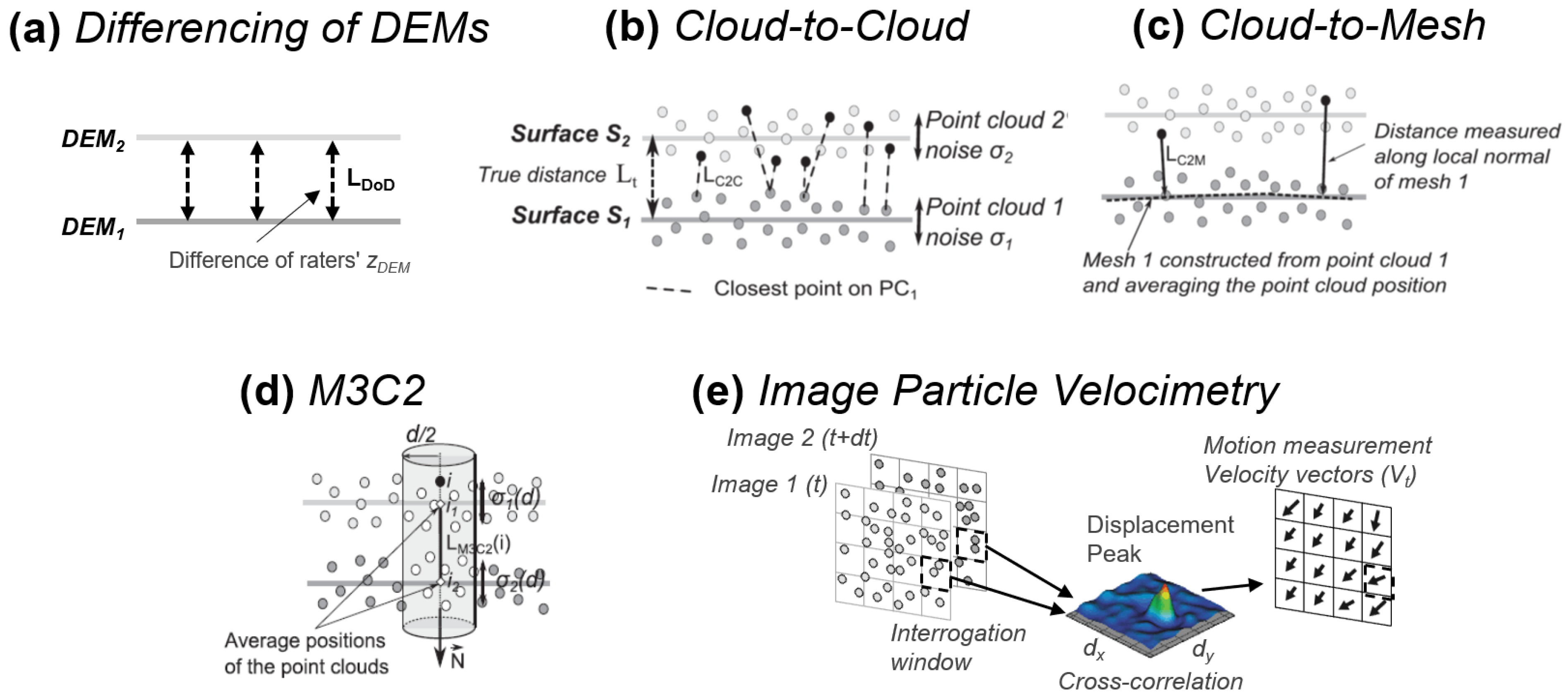
Figure 1. Comparison of common change detection methods including (a) differencing of DEMs, with distances computed vertically. (b) Cloud-to-cloud (C2C) distances are computed based on closest point distance (LC2C). (c) Cloud-to-mesh (C2M) is computed between closest points along the local normal of the mesh (LC2M). (d) Multiscale Model-to-Model Cloud Comparison (M3C2) is computed trough a cylindrical axis, which gives a mean distance along the normal direction ((bd) adapted from [20]). (e) Image Particle Velocimetry (IPV) computes velocity vectors (Vt) from pair image cross correlation.
Drones 07 00258 g001
Figure 2. UAS-derived surface velocity fields of the calving front of the Bowdoin Glacier in 12 h intervals revealed enhanced glacier velocity acceleration over short periods as well as pulsating water flow plumes at the front of the tide-water glacier. Figure adapted from [13].
Drones 07 00258 g002
Figure 3. High temporal monitoring of calving front dynamics by Adams et al. [52]. RGB images (ac) of the calving zone time-series where authors observed increased deformation (df) and velocity (gi) in the hours prior to calving with rates of 24 m day-1.
Drones 07 00258 g003
Figure 4. Seasonal surface dynamics in saturated soils from a road embankment depict uplift and settlement up to 50 cm from soil injection ice development. Inset A provides an example of a surface crack. Inset B shows an area of settlement that was affected by equipment that works to keep the road free of ice in winter. Figure adapted from [65].
Drones 07 00258 g004
Figure 5. (a) Kilauea lava flow site. Standing waves appear as undulations in the channel surface (see A-A′ profile in (e)). (b) UAS hover video frame highlights flow through the channel that is focused on the east side. The standing waves appear as dark and light bands where the crust compresses on up-wave side and pulls apart at the top and down-wave side. (c) Velocimetry analysis comparing features from video using particle image velocity for flow volume and discharge rate estimation. (d) Flow velocity profile from B-B′ across site B as shown in (c). (e) De-trended July 2018 LIDAR channel surface profile from A-A’. Figure adapted from [77].
Drones 07 00258 g005
Figure 6. (a) Deformation and (b) normal strain plot (normal in the image plane) for the lava dome expansion over the course of 3 days, showing significant movement of the northeast dome side, as well as extending radial fractures near the lava flow vent. The arrow length in (a) shows the measured displacement. Survey C was performed on 15 February 2019 at 15:20–15:33 UTC and survey D on 18 February 2019 at 14:38–14:50 UTC. The lava flow and crater rim are marked for orientation and (b) also includes a thermal view on the vent (red circle), also captured on 18 February 2019 at 11:49–12:19 UTC. This shows that active structures of the lava flow produce significant thermal anomalies, although the radial fractures associated with the slower dome growth are not visible. The lava flow and crater rim are marked for orientation, and the reference point for the shift and rotation correction is marked in (a). Figure adapted from [78].
Drones 07 00258 g006
Figure 7. Short temporal scale monitoring captures rapid shoreline change, six times faster than the long-term trend (1952–2017) in Herschel Island, Yukon Territory, Canada. Figure adapted from [82].
Drones 07 00258 g007
Figure 8. Seasonal evolution of coastal bluff mass wasting where wave energy combined with weakening of bluff sediment and thawing in the spring results in substantial bluff erosion as shown in C. (A) May to September 2018, (B) September to December 2018, and (C) December to May (Spring) 2019. Figure adapted from [23].
Drones 07 00258 g008
Figure 9. High resolution (2 cm) interannual monitoring of progradation of dune system revealed the formation of embryo dunes near the shoreline (highlighted yellow A) and the dynamic nature of the system with zones B and C showcasing a seaward displacement of the dune system. Figure adapted from [87].
Drones 07 00258 g009
Figure 10. Assessment of pre and post hurricane gully erosion (a) in the valley of volcan de Colima, western Mexico, with engraving reaching 5 m within a 4-day period based on high resolution repeat photogrammetry terrain modeling (b) and field inspection (c). Figure adapted from [97].
Drones 07 00258 g010
Figure 11. Seasonal landslide displacement magnitude in color. White vectors indicate displacement direction employing a COSI-Corr algorithm. Figure adapted from [40].
Drones 07 00258 g011
Figure 12. Mapping boulder displacement associated with coastal storms. Numbers indicate the approximate masses in tons and arrows connect the initial and final locations of boulders. Figure adapted from [33].
Drones 07 00258 g012
Figure 13. Horizontal displacement from underground mining activities captured from UAS orthomosaics at mm resolution. Figure adapted from [43].
Drones 07 00258 g013
Figure 14. Vertical and horizontal displacements shown by vectors between pre- and post-explosion depicting subtle surface changes and unique morphological signatures for two different experiments: SPE-5 (a) and SPE-6 (b). Figure from [16].
Drones 07 00258 g014
Figure 15. Meta-analysis of change detection studies employing UAS-based photogrammetry, TLS, and ALS depicting niche differences in spatial and temporal scales of geomorphic change detection. Lines merge at the average point for each method. See Table S1 for a full list of studies.
Drones 07 00258 g015
Figure 16. UAS spatial and temporal resolution for the major Earth science fields. Dashed line indicates average of all fields. See Table S1 for list of studies.
Drones 07 00258 g016
Table 1. Common change detection methods used in assessing earth surface processes.
MethodReferenceApplication Examples
DEM of Difference (DoD)Wheaton [22][23,24,25]
Cloud-To-Cloud (C2C) distanceGirardeau-Montaut et al. [26][27]
Cloud-To-Mesh (C2M) distanceCignoni et al. [28][29,30]
Mesh-To-Mesh (M2M) distanceAspert et al. [31][32,33]
Multiscale Model-to-Model Cloud Comparison M3C2Lague et al. [20][34,35,36,37,38]
Coregistration of Optically Sensed Images and correlation (COSI-Corr)Leprince et al. [39][40,41,42,43]
Particle Image Velocimetry (PIV)Keane et al. [44][13,45]
Disclaimer/Publisher’s Note: The statements, opinions and data contained in all publications are solely those of the individual author(s) and contributor(s) and not of MDPI and/or the editor(s). MDPI and/or the editor(s) disclaim responsibility for any injury to people or property resulting from any ideas, methods, instructions or products referred to in the content.

