A Deep Learning Approach for Wireless Network Performance Classification Based on UAV Mobility Features

Abstract

The unmanned aerial vehicle (UAV) has drawn attention from the military and researchers worldwide, which has advantages such as robust survivability and execution ability. Mobility models are usually used to describe the movement of nodes in drone networks. Different mobility models have been proposed for different application scenarios; currently, there is no unified mobility model that can be adapted to all scenarios. The mobility of nodes is an essential characteristic of mobile ad hoc networks (MANETs), and the motion state of nodes significantly impacts the network’s performance. Currently, most related studies focus on the establishment of mathematical models that describe the motion and connectivity characteristics of the mobility models with limited universality. In this study, we use a backpropagation neural network (BPNN) to explore the relationship between the motion characteristics of mobile nodes and the performance of routing protocols. The neural network is trained by extracting five indicators that describe the relationship between nodes and the global features of nodes. Our model shows good performance and accuracy of classification on new datasets with different motion features, verifying the correctness of the proposed idea, which can help the selection of mobility models and routing protocols in different application scenarios having the ability to avoid repeated experiments to obtain relevant network performance. This will help in the selection of mobility models for drone networks and the setting and optimization of routing protocols in future practical application scenarios.

1. Introduction

The mobile wireless network is a self-organized, centerless, dynamic topology, and mobile distributed network, which has the advantages of strong mobility, fast networking speed, the ability to adapt to harsh environments, and strong robustness [1]. It is widely used in fields such as disaster reconstruction, UAV scientific research, military warfare, and other fields. Nodes’ mobility is one of the most significant characteristics of UAV ad hoc networks [2]. Various performance indicators of the network, such as throughput, transmission delay, and routing effectiveness, are closely linked to the mobility of nodes. In UAV wireless networks, node mobility can bring greater sensing ranges, more opportunities for information interactions, and more flexible network services and applications [3]. However, node mobility also brings many problems. The movement of nodes can lead to frequent changes in network topology, which directly affects network performance, such as energy consumption, communication capacity, routing performance, etc., specifically reflected in packet loss, throughput reduction, and even network segmentation. To simulate the complex and variable motion states of nodes, mobility models are therefore proposed to describe the movement patterns, such as node position coordinates, movement speed, acceleration changes, and other information, which is an abstraction of the motion of nodes. Currently, a variety of node mobility models have been proposed, and studies have shown that different mobility models have different effects on the performance of the network protocols and algorithms [4]. As the basis for performance evaluation and network designing of related systems, protocols, and algorithms in mobile ad hoc networks, the research on network node mobility models is of great importance for improving UAV network performance.

Mobility models are important baselines in network simulation to describe the movement of nodes, including changes in their position, velocity, and acceleration. The design and research of mobility models serve as the foundation for the development and application of various protocols and technologies in UAV ad hoc networks, which will help researchers gain a better understanding of network performance and potential issues, thereby promoting the specific implementation and performance improvement in networks. In the research process of mobility models, it is common to introduce or propose a mobility model, then analyze the various characteristics of the model combined with specific connectivity evaluation methods to conduct a theoretical analysis or verify through experiments, and finally, obtain the network connectivity performance under the mobility model [5]. Ref. [6] brought forth a metric, the lifetime of link topology, to evaluate the dynamic characteristics of an ad hoc network. From the analysis of the simulation data of three classical mobility models, it can be seen that the link topology snapshots method is not only a new idea to obtain the link topology lifetime of an ad hoc network but also the ratio of link connection, the variety ratio of link topology, and the link topology lifetime curve could be derived. The movement of nodes in a network mainly depends on the network’s mobility model. In the early days, the random waypoint (RWP) model [7], the random walk (RW) model [4], and other mobility models were often used to simulate the movement of nodes to analyze the relevant characteristics of the network. Ref. [8] analyzed network connectivity performance based on the RWP model and provided an approximation of the probability that the network becomes k-connectivity. In addition, it was also found that when the network is sparse, the mobility of nodes has a positive impact on the connectivity probability of the network, while for dense networks, the opposite is true. Meanwhile, the average connection time of a network also greatly affects network connectivity probability. Based on percolation theory, Ref. [9] studied the maximum connected component in MANETs, using the proportion of the maximum connected component as an important indicator to measure network connectivity; Ref. [10] analyzed the network connectivity of MANETs under the RWP mobility model and obtained the optimal communication radius of nodes when the network satisfies k-connectivity, which is of great significance for improving the robustness and survivability of the network. Reference [11] investigated three connectivity indicators of MANETs, including node degree, average node degree, and maximum node degree, under shadowing effects, and the results provided important insights into improving connectivity and optimizing routing protocols in shadowing environments. Most of the existing research focuses on establishing different node distribution computing models to analyze the characteristics of the network. Currently, most studies on the design of indicators for describing node mobility in mobile models are relatively simple and mostly consist of the same type of indicators. The computational and analytical complexity of the mathematical models is relatively high and is only applicable to a single mobility model in most cases. Owing to the lack of generality, it is difficult to accurately quantitatively analyze or compare the characteristics of various mobility models. On the other hand, the analysis of the impact of mobility on network performance and the relationship between different mobile models is mostly qualitative. For example, in [5], each mobile scenario corresponds to one curve in network performance. If the movement scenario is more complex, a large number of simulation experiments are required to obtain the relevant results.

Deep learning (DL) is a hot research topic in the field of modern computer science [12]. It has been decades of development, from theoretical research to industrial applications. DL has obvious advantages in solving problems with complex model building. Compared to traditional machine learning (ML) algorithms [13], it can automatically learn the deep-seated characteristics of the data. Nowadays, it has been widely used in biomedical, natural language processing, image recognition, and other areas. In the field of communication, introducing DL technology into diverse aspects of wireless communication has been proven to significantly improve the performance of wireless communication systems [14,15,16,17,18]. Compared with other intelligent optimization algorithms, neural networks have the benefits of nonlinearity, input–output mapping, adaptability, fault tolerance, high-speed parallelism, and self-learning, which will definitely provide critical technical support for the development of wireless communication.

The UAV mobile wireless network is a large and complex system; the indicators that can be utilized to describe node motion relationships are complex and diverse, which also have correlations, diversity, and ambiguity characteristics between them [19]. Quantitative or qualitative analysis of network performance is complicated and generally less applicable by using these methods. Therefore, our research proposes a backpropagation-neural-network-based [20] network performance classification method (BPNN-PC). Based on the construction of motion indicators for mobility models, our approach uses five designed motion parameters as inputs to the BP neural network, and the performance of the network under the same motion parameters is introduced as labels to conduct training of the BP neural network, Finally, the BP neural network is used to map the relationship between the mobility index values and the network performance. It can solve the problems of traditional mathematical derivation-based methods, which rely on mobility model types, overly intricate descriptions of relationships between indicators, and low generalization. The final trained BPNN-PC model can output the current status of network performance in different UAV nodes motion scenarios, which is able to assist the selection of UAV network mobility models and the setting or optimization of routing protocols in practical application scenarios using less simulation and calculation.

2. Materials and Methods

2.1. Mobility Model

Considering the application and task scenarios, we have chosen the ‘’Low, slow, and small” drones as our research objective to set the mobility parameters. Among the existing mobility models, the random waypoint mobility model (RWP) [7], the Gaussian–Markov mobility model (GM) [21], and the reference point group mobility model (RPGM) [22] are often used for wireless network protocol performance analysis, routing algorithm design and optimization, network energy consumption, and capacity design [23]. Therefore, we use these representative mobility models to study the mobility characteristics of nodes and the impact of node mobility on the topology characteristics of UAV networks. The following parts describe three mobility models in detail.

2.1.1. Random Waypoint Mobility Model

The RWP [7] model is one of the most widely used node mobility models. Due to its simplicity and practicality, it quickly became the benchmark for evaluating MANET routing protocols [24]. In RWP, nodes that follow a uniform or normal distribution randomly choose the speed $v\in [V_{\min },V_{\max }]$ and direction $\theta \in [0,2\pi ]$ from their initial position. After running for a fixed time interval Δt, they will select a new speed and direction to move until the simulation ends; the motion trajectory of the node is shown in Figure 1. When initializing the network, the state and position of nodes are randomly initialized, so at the beginning, the nodes are evenly distributed throughout the entire movement area [25]. The endpoint of each motion of a node is a random location in the entire region; the speed of node movement is also randomly selected within a certain range. The model is a simple random mobility model, but according to existing simulations, there are many sharp turns in the model, which is one of the shortcomings of the model. The model is also a memoryless mobility model. The selection of node speed and direction has no correlation with the previous speed and direction, and it will move along a new route. At the same time, if the time interval or moving distance is too small, the nodes will basically move in a small area, unable to traverse various states, resulting in the uneven spatial distribution of nodes. The following is the relationship between the coordinates $\left(x_n,y_n\right)$ of the node during the n-th movement and the coordinates $\left(x_{n-1},y_{n-1}\right)$ during the n-1st movement:

$$x_n=x_{n-1}+v_{n-1}\cos {\theta }_{n-1}$$

(1)

$$y_n=y_{n-1}+v_{n-1}\sin {\theta }_{n-1}$$

(2)

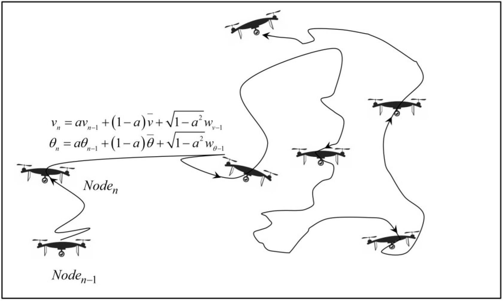
2.1.2. Gaussian–Markov Mobility Model

When the movement of a node is time-dependent, it means that the movement of the node is governed by the laws of physical kinematics, and the movement of the current moment is closely related to the movement of the previous moment. For example, the current speed of a node depends on the speed of the previous moment, and in most cases, the node moves along a given path. Gaussian–Markov (GM) [21] model was originally proposed to implement the simulation of personal communication systems. GM models can be used in networks to capture the correlation between the time and speed of nodes.

In this model, each node is initially assigned a velocity, including the value of velocity v and direction θ. For every fixed time interval Δt, the node updates the speed and direction once, and this update is based on the previous update. The calculation formula is as follows:

$$v_n=a{v}_{n-1}+\left(1-a\right)\overline{v}+\sqrt{1-a^2}{w}_{v-1}$$

(3)

$${\theta }_n=a{\theta }_{n-1}+\left(1-a\right)\overline{\theta }+\sqrt{1-a^2}{w}_{\theta -1}$$

(4)

where $\overline{v}$ and $\overline{\theta }$ are the mean values of the velocity and direction when n approaches infinity, respectively; $w_{v-1}$ and $w_{\theta -1}$ are two unrelated Gaussian random variables with a mean α value of 0 and a variance of 1; and α is an adjustable parameter within the range of [0, 1] to control the randomness of the nodes. By adjusting the value of α, the strength of the node motion correlation can be adjusted. At the n-th time interval, the current position of the node can be obtained using Formulas (1) and (2). The motion trajectory of the node is shown in Figure 2.

The model effectively solves the phenomenon of the sudden turning of nodes in a random mobility model, which is more in line with the movement of entities. However, in GM, the speed of a node at any time interval is a dependent Gaussian variable of the speed of the previous time interval, which makes it impossible to maintain the motion trajectory in a straight line under certain parameters, and the entire simulation process does not pause, which is inconsistent with the movement of UAVs in reality [3].

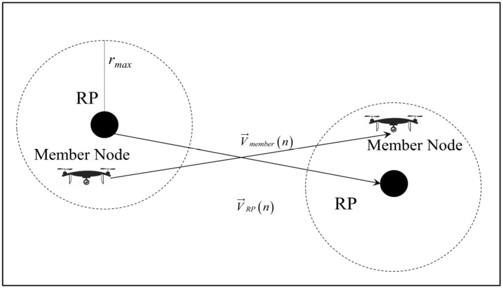
2.1.3. Reference Point Group Mobility Model

The reference point group mobility model [22] is one of the group models. In this model, each group has a reference point (RP), and the path of group members’ movement is determined by the RP. Each movement of group members is a random offset from the RP. The RPGM model is the most commonly used group mobility model, composed of one or more groups of nodes with a logical center. In the model, each group’s logical center’s motion mode determines the entire group’s motion mode, including position, velocity, direction, and acceleration. The positions of other nodes in the group will change with the position of the logical center. The RPGM model can fully describe this movement trend of nodes in a network. However, it still has the following drawbacks: When using a reference point group mobility model, we need to master the information of all nodes. The drone swarm network is distributed, and the network topology undergoes high-speed dynamic changes. It is basically impossible to obtain all the information of nodes in the network [26].

The RPGM model is shown in Figure 3. A random value of velocity and direction are generated for each node member of the group evenly at each time interval Δt. The movement of nodes in this model includes group movement and individual movement. The movement of RP and the random movement of members constitute two parts of individual movement. Generally, members are evenly distributed within a group, and each member is assigned an RP to form a group for movement. Specifically, each node member allows independent movement around the RP for each group. If the speed of RP is ${\overrightarrow{V}}_{RP}\left(n\right)$ at time n, the speed of any of its member nodes is

$${\overrightarrow{V}}_{member}\left(n\right)={\overrightarrow{V}}_{RP}\left(n\right)+\overrightarrow{R_n}$$

(5)

where $\overrightarrow{R_n}$ is a random vector offset of the member node relative to its RP, with a value between [0, r_max]; r_max is the maximum offset distance defined; and the direction of $\overrightarrow{R_n}$ is a random value between [0, 2π]. The main application case of RPGM is the logical relationship between officers and soldiers in military communications. This article selects the RPGM model as a typical representative of the spatial dependency model.

2.2. Mobility Indicator Design

As mentioned above, the primary task of establishing a mobility model is to provide the mobility scenarios required for network simulation by correctly and reasonably describing the node mobility manners. Are there any differences in the scenarios provided by different mobility models? What are the unique aspects? Does network performance vary depending on how UAV nodes move? If so, how to measure its impact, and so on, all of these issues involve correctly measuring and evaluating the motion of mobility models. The speed of movement and communication radius of a node directly affects the establishment of a communication link. During the movement of a single node, not only the movement relationship between two nodes will change, but also the movement state of a single node will affect the global connectivity and the structure of the graph. Therefore, our research considers the motion relationship between nodes when describing the motion performance of a mobility model. At the same time, the motion nodes in a network can be described as points by using graph theory, the link between two nodes can be described as the edge, and global connectivity characteristics of the network can be abstractly described as a graph. By analyzing the graph’s characteristics, we also establish global motion characteristics description indicators.

Firstly, we show the definitions and symbolic expressions of the following variables:

• Ÿ Node s is the source node, node d is the destination node for forwarding, and R is the communication radius of the node.
• $l_{x,y}(t)$ indicates the Euclidean distance between node x and node y at time t.
• $\overrightarrow{V_x}\left(t\right)$ represents the velocity vector of node x at time t; and $\left|{\overrightarrow{V}}_x(t)\right|$ represents the velocity value of node x at time t.
• $x_x\left(t\right)$ represents the x coordinate of node x at time t; and $y_x\left(t\right)$ represents the y coordinate of node x at time t.
• $RD\left({\overrightarrow{v}}_x\left(t\right),{\overrightarrow{v}}_y\left(t\right)\right)$: the relative direction (RD), or cosine of the angle between two velocity vectors, calculated by $\frac{{\overrightarrow{v}}_x\left(t\right),{\overrightarrow{v}}_y\left(t\right)}{\left|{\overrightarrow{v}}_x\left(t\right)\right|\ast \left|{\overrightarrow{v}}_y\left(t\right)\right|}$.
• $VR\left({\overrightarrow{v}}_x\left(t\right),{\overrightarrow{v}}_y\left(t\right)\right)$: the velocity ratio (VR) between two vectors, calculated by $\frac{\min \{\left|{\overrightarrow{v}}_x\left(t\right)\right|, \left|{\overrightarrow{v}}_y\left(t\right)\right|\}}{\max \{\left|{\overrightarrow{v}}_x\left(t\right)\right|, \left|{\overrightarrow{v}}_y\left(t\right)\right|\}}$.
• Ÿ N: number of mobile nodes.
• Ÿ T: time of nodes motion duration.

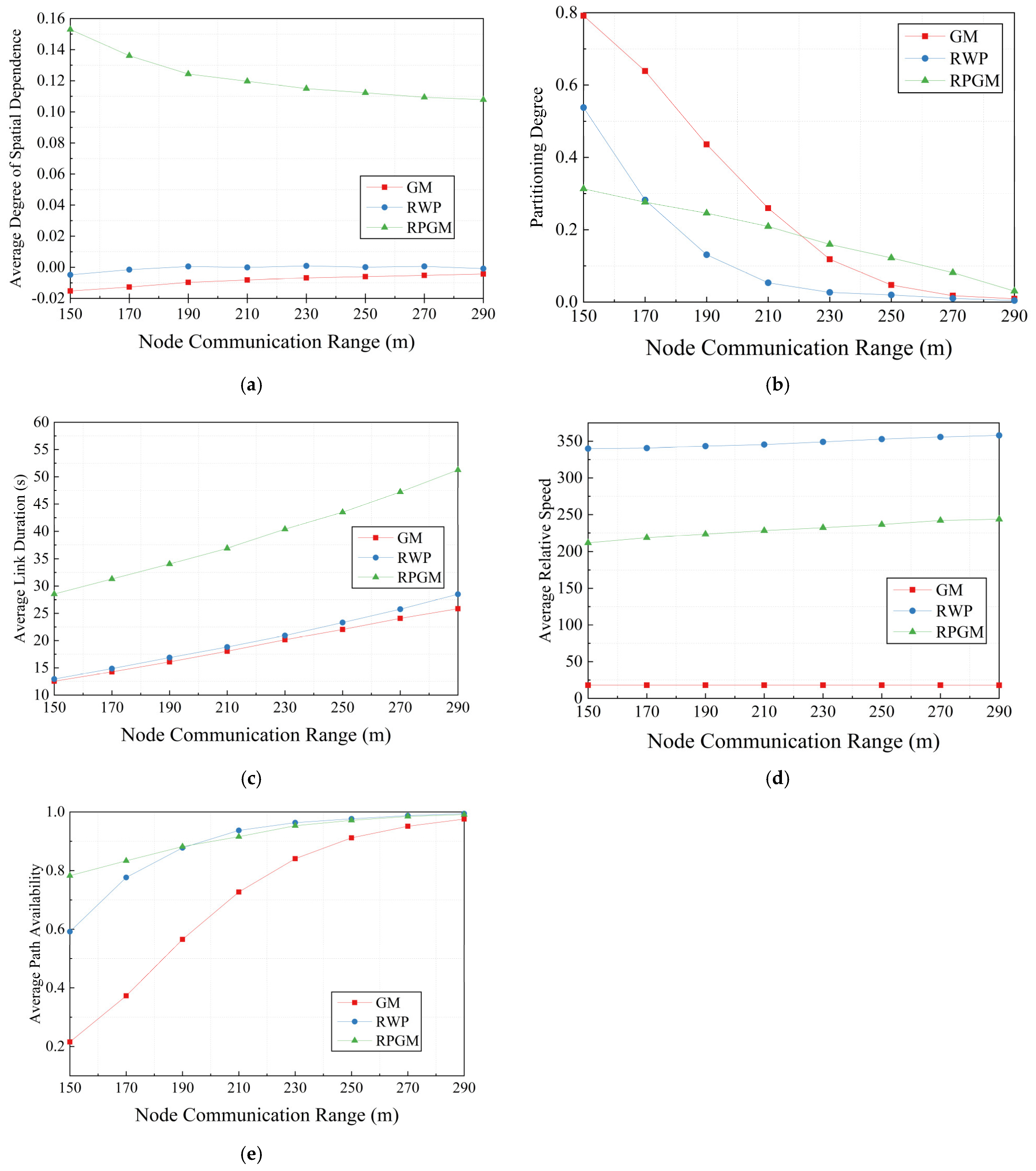
2.2.1. Spatial Dependency

We use spatial dependency (SD) to describe how much the movement of nodes is affected by each other. It is the speed similarity of two nodes that are not too far apart, which can be defined as follows:

$$D_{spatial}\left(x,y,t\right)=RD\left({\overrightarrow{v}}_x\left(t\right),{\overrightarrow{v}}_y\left(t\right)\right)\ast VR\left({\overrightarrow{v}}_x\left(t\right),{\overrightarrow{v}}_y\left(t\right)\right)$$

(6)

When node x and node y move in approximately the same direction and at almost similar speeds, the value of $D_{spatial}\left(x,y,t\right)$ is higher. However, if the ratio of relative direction or speed decreases, the value of $D_{spatial}\left(x,y,t\right)$ will decrease.

Since the motion of nodes rarely depends spatially on nodes that are farther away, the following conditions are added:

$$l_{x,y}\left(t\right)>\alpha \ast R\Rightarrow D_{spatial}{\left(x,y,t\right)}_{}=0$$

(7)

As can be seen from [27], for a value of a = 2, $D_{spatial}\left(x,y,t\right)$ can very clearly distinguish different mobility patterns. The average value of $D_{spatial}\left(x,y,t\right)$ at a specific time of a node pair is calculated as follows:

$$\overline{D_{spatial}}=\frac{{{\displaystyle \sum }}_{t=1}^T{{\displaystyle \sum }}_{x=1}^N{{\displaystyle \sum }}_{y=x+1}^N{D}_{temporal}^{}\left(x,y,t\right)}{P}$$

(8)

where P is the number of tuples $\left(x,y,t\right)$ that make $D_{spatial}\left(x,y,t\right)\ne 0$. Therefore, if the mobile nodes move independently of each other, the $D_{spatial}\left(x,y,t\right)$ value of the mobility model will be smaller. On the other hand, if node movements are coordinated by a central entity or influenced by nearby nodes, making them move in similar directions and speeds, the $D_{spatial}\left(x,y,t\right)$ value of the mobility model will be higher.

2.2.2. Partitioning Degree

Partitioning degree (PD) is used to describe the probability that two randomly selected nodes are not within the same connection component at a randomly selected time t. Because the network topology is mostly connected during the movement process, that is, for any pair of nodes, there is at least one fully connected path between them. In scenarios with more intense movement, the network topology may be divided into several disconnected sub-regions, and two nodes may locate in different sub-regions, causing network partitioning and routing algorithms to fail to work properly.

Let $G=\left(V,E\right)$ represent a graph of V nodes and E edges. There are k partitions $V_1,\cdots ,V_k$ that $V_1\cup V_2{\cup }_{\cdots }{V}_k=V$, and $V_i\cap V_j=\varnothing ,i\ne j$. At time t, if two nodes x and y lie in the same sub-region $V_i$, $Pd=0,x,y\in V_i$; else, $Pd=\mathrm{Pr}[x\in V_i]\mathrm{Pr}[y\in V_j], i\ne j$.

2.2.3. Link Duration

The link duration (LD) is the link’s average duration between two nodes x and y. It is a measure of link stability between nodes, which can be calculated as follows:

$$LD\left(x,y\right)=\left\{\begin{array}{cc}\frac{{{\displaystyle \sum }}_{t=1}^{T}C\left(x,y,t\right)}{linkchange\left(x,y\right)}\hfill & \hfill linkchange\left(x,y\right)\ne 0\\ {{\displaystyle \sum }}_{t=1}^{T}C\left(x,y,t\right)\hfill & \hfill otherwise\end{array}\right.$$

(9)

In which $C\left(x,y,t\right)$ is the indicator random variable which has a value of 1 if there is a link between nodes x and y at time t, otherwise it is 0, and $linkchange\left(x,y\right)$ is the number of link changes for a pair of nodes x and y, which is the number of times the link between them transitions from “down” to “up”.

2.2.4. Relative Speed

The relative velocity between node x and node y is defined as $v\left(x,y,t\right)$:

$$v\left(x,y,t\right)=\frac{d}{dt}\left(nod{e}_x\left(x_x(t),y_x(t)\right)-nod{e}_y\left(x_y(t),y_y(t)\right)\right)$$

(10)

The relative speed (RS) between any pair of nodes (x, y) is defined as the absolute value of their relative velocity, which is taken as the average value over the time T for measuring mobility. The formula is as follows:

$$R{S}_{nod{e}_x,nod{e}_y}=\frac{1}{T}{\displaystyle \underset{0\le t\le T}{\int }\left|v\left(x,y,t\right)\right|dt}$$

(11)

2.2.5. Path Availability

Path availability is a portion of the path availability time between two nodes x and y:

$$PA\left(x,y\right)=\left\{\begin{array}{cc}\frac{{{\displaystyle \sum }}_{t=star{t}_{(x,y)}}^{T}A\left(x,y,t\right)}{T-start\left(x,y\right)}\hfill & \hfill T-start\left(x,y\right)>0\\ 0\hfill & \hfill otherwise\end{array}\right.$$

(12)

where $A\left(x,y,t\right)$ is a random variable, such that if the path from node x to node y is available at time t, its value is 1; otherwise, its value is 0. $start\left(x,y\right)$ is the start time of communication service between nodes x and y.

Average path availability is the average value across pairs of nodes that meet specific conditions.

$$PA=\frac{{{\displaystyle \sum }}_{x=1}^N{{\displaystyle \sum }}_{y=x+1}^{N}PA\left(x,y\right)}{P}$$

(13)

In which P is the number of node pairs (x, y) that satisfy $T-start\left(x,y\right)>0$.

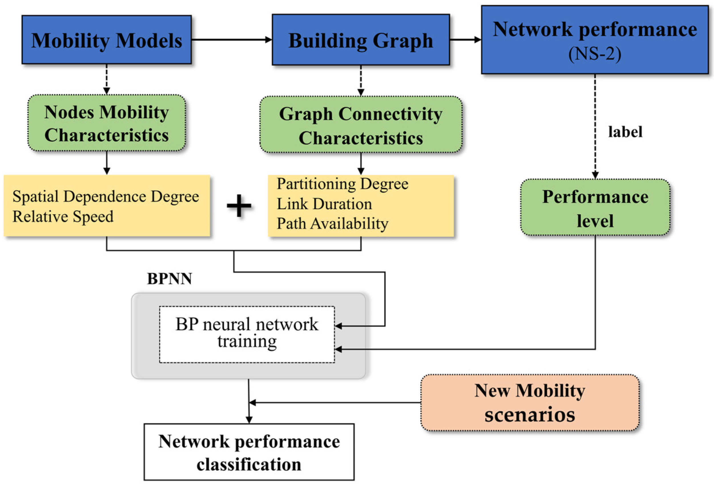
2.3. Neural Network Architecture

BP neural network [20] is the most basic neural network, which can learn and store a large number of input–output mapping relationships without revealing the mathematical equations in advance. The learning process consists of two parts: forward propagation of signals and backpropagation of errors. Its learning rule is to use the steepest descent algorithm to continuously adjust the weights and thresholds of the network through backpropagation to minimize the sum of square errors of the network. Due to the effective function approximation ability of the BP neural network, we built a BPNN to map the correlation between the five motion feature parameters of the mobility model defined in Section 2.2 and network performance. The basic structure of the BP neural network is shown in Figure 1. Our BPNN is composed of an input layer, three hidden layers, and an output layer. Each neuron algebraically sums the weighted input and the threshold (offset) vector to obtain its own output.

The input layer of the neural network is $x=(x_0,x_1,x_2,x_3,x_4)$, where $x_0,\cdots ,x_4$ are five motion metrics designed in Section 2.2. The number of hidden layers in the BP neural network used in our design is 3, and each layer contains 32, 48, and 16 neurons, respectively. Finally, the number of neurons in the output layer is 8, $y=(y_0,y_1,y_2,y_3,y_4,y_5,y_6,y_7)$, where y_i represents different network performance levels. Relu [28] activation function is used between the input layer and the hidden layer, and LogSoftmax is used as the activation function between the last hidden layer and the output layer.

For hidden layers, the input is

$$i_j={\displaystyle \sum _{i=0}^4{w}_{ij}{x}_i+b_j,j=0,\cdots n}-1$$

(14)

where n is the number of neurons in the current layer, w_ij is the weight coefficient, and b_j is the bias coefficient. If the activation function is f(x) = ReLU, the output of this hidden layer is

$$o_j=f(i_j)$$

(15)

Then o_j continues to be propagated forward as input to the next hidden layer.

To avoid the overfitting problem of BPNN, different parameter combinations need to be used to test and screen the best network model. Due to the different ranges of input and output variables, it is necessary to standardize the values of the dataset by using the normalization method to process input and output data. In addition, to ensure an accurate evaluation of the classification ability of the constructed model, the dataset is randomly divided into the training set and the validation set. Owing to the random partitioning of the dataset, both the validation and training sets contain collected data under different node motion states. Among them, the training set accounts for 80%, and the validation set accounts for 20%.

3. Experiments and Settings

Our experiment is mainly divided into three parts. Firstly, the generation and recording of node motion scenes are carried out in BonnMotion [29]. Based on this, mobility data analysis is carried out to obtain the actual values of the five motion indicators of the mobility model in different scenarios; secondly, Network Simulator 2 (NS2) [30] is used to build a wireless network environment and conduct network performance tests. After deploying the nodes and network architecture, we use the motion scene files generated in the first step to test and record network performance in sequence by writing test scripts. Finally, we design and implement the BPNN network proposed in Section 2.3, process the obtained data accordingly, and input it into the neural network for training. The flowchart of the entire process is shown in Figure 4 below.

3.1. Experimental Settings and Data Preparation

The number of mobile nodes in our simulation is 40, and the movement area is a rectangle area of 1 km * 1 km. The nodes use the above three movement models to move, with a speed of 0–140 m/s with a 10 m/s speed interval. In order to reduce the impact of randomness on the experiment, 60 random seeds are set for each model in the same speed interval to randomize the parameters in the network, and the communication radius of the nodes varies between 150 m and 290 m. Under Ubuntu 16.04 operating system, a “.sh” script file is written in the Bonnmotion software directory to simulate the above motion scenario in batches. The command in .sh file: “/home/bonnmotion-3.0.1/bin/bm -f GM_$m$h-$rr GaussMarkov -n 40 -d 500 -b -x 1000 -y 1000 -i 0 -b -g -m $m -h $h” is used to generate the motion scenario of the Gaussian Markov model. “-n” represents that there are 40 nodes; “-d” represents that the simulation time is 500 s; “-x, -y” is the range setting of the simulation area; “m” is the lower limit of the speed interval, “h” is the upper limit of the speed interval, and “rr” is the random seed variable. Then, the generated mobility model files are converted into an NS2-usable mobility files using the command: “/home/bonnmotion-3.0.1/bin/bmNSFile -f GM_$m$h-$rr”.

We tested and calculated the values of the parameters varying with the communication radius in the speed range of 0–20 m/s, as shown in

Table 1. Mobility parameters value of three mobility models.

Mobility Models	R	Spatial Dependency	Partitioning Degree	Link Duration	Relative Speed	Path Availability
GM	150 m	−0.015215	0.79171	12.54591	17.91827	0.215451
	170 m	−0.012723	0.63871	14.25538	17.92939	0.3729329
	190 m	−0.009718	0.43584	16.08956	17.91865	0.5653631
	210 m	−0.008186	0.25967	18.04655	17.89447	0.7269393
	230 m	−0.006838	0.11843	20.15201	17.88892	0.8405965
	250 m	−0.006032	0.04717	22.04167	17.89431	0.9115855
	270 m	−0.005227	0.01758	24.07127	17.88145	0.9512641
	290 m	−0.004291	0.00908	25.84114	17.8526	0.975736
RWP	150 m	−0.004837	0.5379	12.94823	339.91358	0.5918288
	170 m	−0.001533	0.28228	14.86327	340.65322	0.7765334
	190 m	0.0005551	0.13087	16.88473	343.33133	0.8776451
	210 m	−6.69 × 10−5	0.05339	18.81895	345.42728	0.9371746
	230 m	0.0008916	0.02679	20.92555	349.1127	0.9635666
	250 m	0.0001047	0.01976	23.31782	352.91237	0.9766939
	270 m	0.0006109	0.01021	25.76445	355.74068	0.9875341
	290 m	−0.000827	0.0042	28.50262	358.01649	0.9942976
RPGM	150 m	0.1529827	0.31306	28.54253	211.58224	0.7826548
	170 m	0.1360633	0.27617	31.30638	218.66965	0.8334138
	190 m	0.1243506	0.24576	34.05127	223.39237	0.8820463
	210 m	0.1196804	0.20896	36.91552	228.24037	0.9156089
	230 m	0.1149647	0.15945	40.39146	232.21462	0.9529495
	250 m	0.1122537	0.12214	43.50398	236.51875	0.9714706
	270 m	0.1093957	0.08126	47.21895	242.02399	0.9846366
	290 m	0.107786	0.03047	51.25484	243.77849	0.990941

. Different parameters exhibit different performances at the same motion speed and R. The trend of the same parameter changing with radius R also varies across different motion models. At the same time, we store and convert all the motion processes into NS2 motion files for subsequent network performance simulation in the same motion scenario. Finally, the data of each speed and index under unique random seed and communication radius are statistically recorded.

To evaluate the effect of mobility on the performance of network protocols, we carried out simulations in the NS2 environment [30] with the wireless ad hoc networking extension. The mobility patterns used were the same as mentioned above. The traffic pattern was generated by the Cbrgen tool of NS2. The traffic consisted of 10 constant bit rate (CBR) flows, of which the source–destination pairs were chosen at random. The data rate used was 4 packets/s, and the packet size was 64 bytes. We evaluated the performance of AODV [31] across this rich set of mobility models and observed that the mobility models might drastically affect protocol performance which will be discussed in detail in the next section. The network parameter settings are shown in

Table 2. Simulation parameter settings.

Simulation Parameter	Value
Transmitter range	150 m–290 m
Bandwidth	2 Mbps
Simulation time	500 s
Number of nodes	40
Speed	0 m/s–140 m/s
Environment size	1000 m × 1000 m
Traffic type	constant bit rate
Packet rate	4 packets/s
Packet size	64 bytes
Number of flows	10
Propagation model	Friis loss model
Transmit power	7.5 dBm

below.

We conducted network simulation and testing using the AODV protocol as an example in the above scenario. Figure 5 displays the result of the network packet delivery ratio obtained from the testing. Among them, we set up four groups for the RPGM model, as the node contact between the groups is relatively close, the change in packet delivery rate of RPGM is relatively small as the motion speed increases, and different communication radii have a small impact on the network performance. GM and RWP’s packet delivery rate decreases significantly with increasing speed and decreasing communication radius. Finally, it can be seen that the packet delivery rate performance of this routing protocol remains above 20%, so we divided the network performance levels with a 10% interval. correspond in sequence to (100%, 90%], (90%, 80%], …, (30%, 20%].

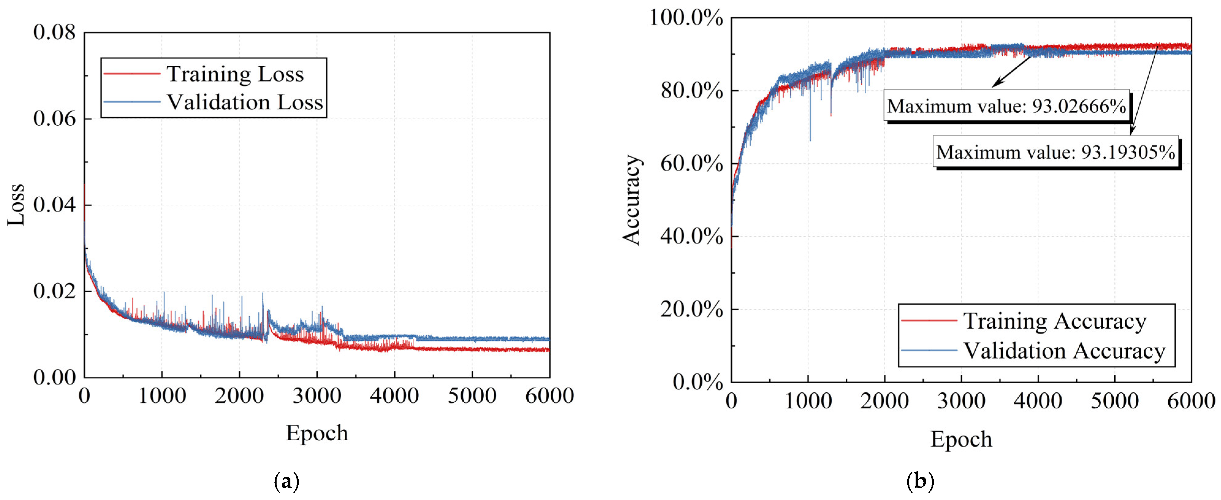
3.2. Training the Network

From the data construction, it can be seen that there are five input features, so the input layer has five nodes. Moreover, there are eight categories of GM network performance; therefore, the output layer has eight nodes. We initialized the parameters (weights, biases) of the BP network. Through forward propagation calculation, that is, iterative calculation from the input layer to the output layer, then predict the type of network performance and compare whether the prediction is correct (calculate the deviation between the predicted value and the true value through the loss function, the smaller the deviation, the closer the classification is to the truth; finally select the optimal parameter and save the neural network model).

There are h (h = 3) hidden layers, and according to the forward propagation order, the number of nodes in each hidden layer is denoted as $m_1,m_2,\cdots ,m_h$; the outputs of each hidden layer are $y^1,y^2,\cdots ,y^h$; and the weight matrices of each layer are denoted as $w^1,w^2,\cdots ,w^h,w^{h+1}$. The neural network framework is built based on PyTorch, and the above neural network is implemented and trained on a CPU (AMD Ryzen 5600H with Radeon Graphics 3.30 GHz). The following Algorithm 1 is the detailed process:

Algorithm 1 The proposed BPNN-based algorithm for the mobility model and network performance evaluation method.

1. Initialization of neural network: random initialize weights and bias; set batch size = 32 and learning rate = 0.004.

2. Input sample data with five features, $x={(x_1,x_2,\cdots ,x_n)}^T,n=5$, and calculate the output for each layer, $y_j=f\left(V_j^{T}X\right)j=1,2,\cdots ,m$ $O_k=f\left(w_j^{T}Y\right)\hspace{1em}k=1,2,\cdots ,l$.

3. Calculate loss: $E=\frac{1}{2}{\displaystyle {\displaystyle \sum }_{p=1}^p}{\displaystyle {\displaystyle \sum }_{k=1}^l}{(d_k^p-O_k^p)}^2$.

4. Calculate loss signals for each layer: $\hspace{1em}{\delta }_k^o=\left(d_k-O_k\right)\left(1-O_k\right)O_k\hspace{1em}k=1,2,\cdots ,l$ ${\delta }_j^y=\left({\displaystyle {\displaystyle \sum }_{k=1}^l}{\delta }_k^o{\omega }_{jk}\right)\left(1-y_j\right)y_j\hspace{1em}j=1,2,\cdots ,m$.

5. Adjusting the weight values of each layer: $\hspace{1em}{\omega }_{jk}\Leftarrow {\omega }_{jk}+n{\delta }_k^o{y}_i (k=1,2,\cdots ,l;j=0,1,\cdots ,m)$ $v_{ij}\Leftarrow v_{ij}+n{\delta }_j^y{x}_i (j=1,2,\cdots ,m;x=0,1,\cdots ,n)$.

6. At the end of the iteration, save the optimal neural network parameters; otherwise, continue with Step 2.

7. End.

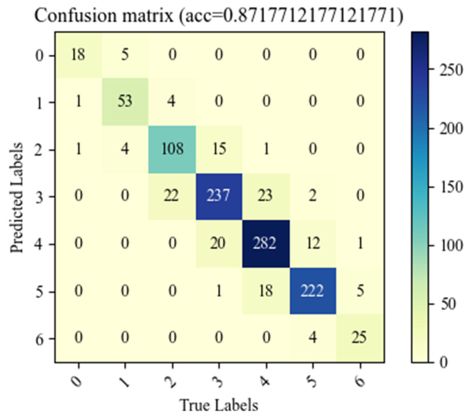
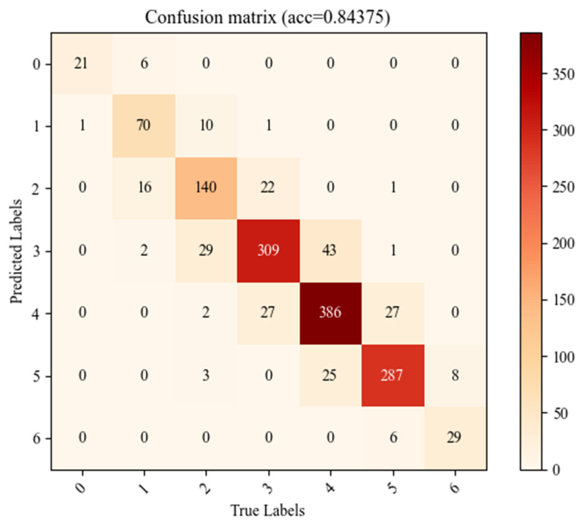
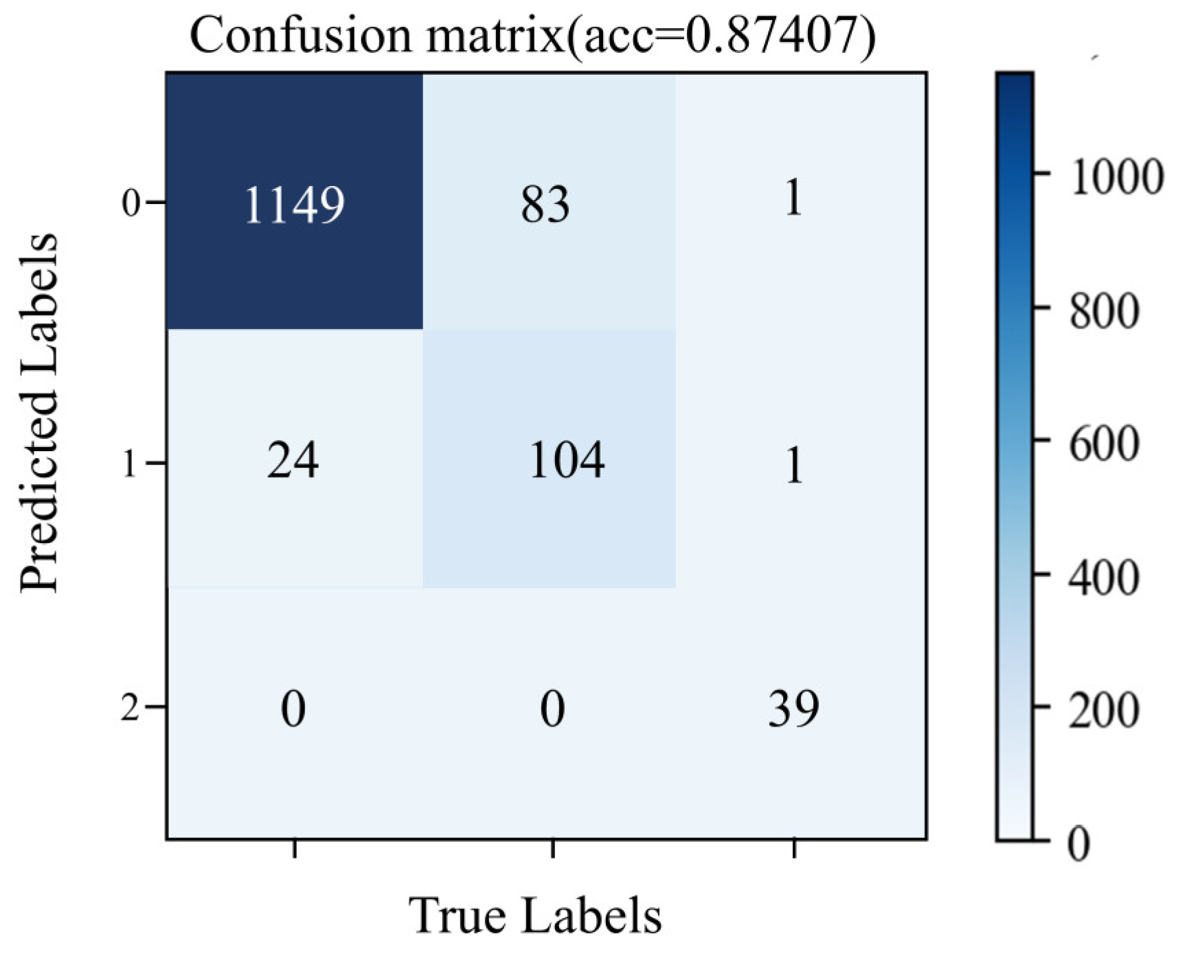
4. Results and Analysis

Firstly, we simulated five motion indicators of three Mobility models and obtained the following performance curves. The communication radius R varies between 150 m and 290 m. Figure 6 shows that as the communication radius increases, the changing trends of the five parameters are different. From Figure 6a, it can be seen that there is no spatial correlation between GM and RWP, which is consistent with the conclusion of [32]. The relative speed remains basically unchanged trend with the increase in node communication radius. However, there are significant differences in this parameter among the three mobility models: the GM with time dependence has the lowest relative speed for a single node, as its motion is time-correlated; the RWP with completely independent motion at each time interval has the highest relative velocity.

The above results show that the performance of the group mobility model RPGM is superior to that of the individual mobility models RWP and GM. In this experimental scenario, 40 motion nodes were divided into 4 groups with 10 nodes in each group, and 9 of them randomly moved around a central node. The nodes were relatively concentrated, and the network’s connectivity performance was good. As the communication radius of nodes increases, the sensing range of nodes becomes larger. The degree of the partitioning of mobility models greatly decreases, available paths increase, and the link duration of mobility models increases, with RPGM greater than RWP and GM. Because GM and RWP nodes are independent of each other, the average spatial dependence of the two is much smaller than that of the group mobility model RPGM which depends on the motion of the head of the node group.

The above indicates that the parameters we selected are basically in line with the motion characteristics of the nodes during the motion process, and the differences between different models can also be reflected in the parameters. Next, we will start training and testing the neural network. Firstly, we collected data from the GM model based on the motion scenario set in Section 3.1. The data were normalized and input into the neural network. The performance of the training and validation sets during the neural network training process is shown in Figure 7.

As the number of training epochs increases, the loss of the test and validation sets shows a decreasing trend and remains stable after 4300 epochs. The maximum value of training accuracy was 93.19305%, and the maximum value of validation accuracy was 93.02666%. In order to verify the generalization of the model, we saved the network parameters with the highest accuracy rate in the training process and then used different motion speeds and random seeds to generate a batch of new GM mobility scenes. After processing the data according to the above process, we used them as the test dataset. After using the test data as the input of the neural network, the accuracy of network performance classification is shown in Figure 8.

Table 3. Confusion matrix of classification results.

Actual Result	Predicted Result
	Positive	Negative
Positive	TP	FN
Negative	FP	TN

is the definition of the randomness and a completely independent confusion matrix, where the initialisms correspond to the following:

True positive (TP) refers to the correct number of positive samples for classification, which are predicted to be positive samples and are actually positive samples.

False positive (FP) refers to the number of negative samples mistakenly marked as positive samples; that is, the actual number of negative samples predicted to be positive samples, so they are false.

True negative (TN) refers to the correct number of negative samples for classification, which are predicted to be negative samples and are actually negative samples.

False negative (FN) refers to the number of positive samples mistakenly marked as negative samples; that is, the actual number of positive samples predicted to be negative samples, so they are false.

TP + FP + TN + FN: total number of samples. TP + FN = P: the actual number of positive samples. FP + TN = N: actual negative sample count. TP + FP: the total number of positive samples predicted, including correct and incorrect predictions. TN + FN: the total number of negative samples predicted, including correct and incorrect predictions.

The indicators below are often used to evaluate the classification performance of classifiers:

• Ÿ Precision: the ratio of the number of samples correctly identified as P to the total number of samples identified as P. In terms of the determined results, this parameter can serve as a basis for determining classification accuracy, reflecting the ability of the neural network to “find the right” positive samples.

$$P=\frac{TP}{TP+FP}$$

(16)

• Ÿ Recall: the ratio of the number of samples correctly classified as P to the total number of real P-class samples. In terms of real samples, this parameter can determine the comprehensiveness of neural networks in sample classification.

$$R=\frac{TP}{TP+FN}$$

(17)

• Ÿ Specificity: the proportion of samples classified to be correct among all negative samples, which measures the neural network’s ability to recognize negative samples.

$$S=\frac{TN}{FP+TN}$$

(18)

The following

Table 4. Three indicators of classification performance.

Network Performance Label	Precision	Recall	Specificity
0	0.783	0.9	0.995
1	0.914	0.855	0.995
2	0.837	0.806	0.978
3	0.835	0.868	0.942
4	0.895	0.87	0.957
5	0.902	0.925	0.972
6	0.806	0.806	0.996

is the performance of three indicators of each category on the test dataset. It can be seen that the trained neural network also performs well on the new data set. The classification accuracy can reach 87.2%, which verifies the feasibility of our idea.

Following the above experimental process, the RWP and RPGM models were subjected to the same experiment, and their performance on their respective test datasets was as follows:

From Figure 5, it can be seen that the overall network performance of RPGM is relatively good. Therefore, in the aforementioned motion scenario, the network performance labels are set to 3 categories: 0, 1, and 2. According to Figure 9, the trained neural network for RWP has the lowest accuracy, approximately 84%, with greater randomness and a completely independent node motion pattern. From Figure 10, it can be seen that even if the number of network classifications (label types) is changed, good classification performance can still be maintained. The classification accuracy of RPGM for the test dataset is 87.407%, further verifying the reliability of network performance classification based on our proposed five indicators for describing motion performance.

Considering the cost issue, researchers are unable to construct actual unmanned aerial vehicle (UAV) networks every time to obtain operational data. It is also difficult to deploy truly controllable UAV mobile networks for performance evaluation. Therefore, in most cases, network planning can only be achieved through simulation platforms. During this process, the choice of the mobility model will directly affect the rationality of network planning and ultimately affect the performance of network information transfer. Moreover, the selection of simulation experiment parameters for nodes’ mobility models also has a significant impact on research results. It can be seen that research on mobile models has extremely important practical significance and application value for the development of UAV wireless network systems. Under different node mobility models, the performance of the same routing protocol varies significantly, so it is crucial to select an appropriate node movement model when conducting UAV routing protocol research.

5. Conclusions

In this study, we use BPNN to explore the relationship between the motion characteristics of mobile nodes and the performance of routing protocol in mobile ad hoc networks. The BP neural network is trained by extracting five indicators that describe the relationship of node-to-node and node–global characteristics. The trained model exhibits good network performance classification accuracy on new datasets with different motion features (different speed range and communication radius), which verifies the correctness of the proposed idea, and provides a certain basis for the improvement and optimization of subsequent routing protocols. Our method also can help the selection of mobility models and routing protocols in different motion scenarios, which will have the ability to avoid a large number of repeated experiments to obtain relevant network performance. By using trained neural networks, the low or good performance of routing protocols under different mobility models can be determined, which can assist in the selection of drone network mobility models in practical application scenarios. The mobility characteristics of nodes have a significant impact on the network topology. The selection of mobility models and their parameters have a significant impact on the simulation results obtained. Therefore, the design and research of mobility models are the foundation for the development and application of various protocols and technologies in UAV networks. It will help us have a better analysis of UAV network performance and potential problems, thereby promoting the specific implementation and performance improvement in UAV networks. Given the unique nature of drone communication nodes, most existing research is based on simulation. Therefore, the evaluation of network performance under a reasonable drone node mobility model is truly reliable. Our work can provide an important basis for the selection of mobility models and the setting of various model parameters in drone networks. In future work, the dynamic graph neural network is planned to be used to model the mobile nodes so as to analyze the time-varying mobility characteristics and network performance of the network at a more fine-grained level, which can also have the ability to obtain the correlation relationship and importance level between various indicators.

References

1. Toh, C.K. Ad Hoc Mobile Wireless Networks: Protocols and Systems; Pearson Education: New York, NY, USA, 2001. [Google Scholar]
2. Khan, M.A.; Safi, A.; Qureshi, I.M.; Khan, I.U. Flying ad-hoc networks (FANETs): A review of communication architectures, and routing protocols. In Proceedings of the First International Conference on Latest Trends in Electrical Engineering and Computing Technologies (INTELLECT), Karachi, Pakistan, 15–16 November 2017; pp. 1–9. [Google Scholar]
3. Kumari, K.; Sah, B.; Maakar, S. A survey: Different mobility model for FANET. Int. J. Adv. Res. Comput. Sci. Softw. Eng. 2015, 5. [Google Scholar]
4. Camp, T.; Boleng, J.; Davies, V. A survey of mobility models for ad hoc network research. Wirel. Commun. Mob. Comput. 2002, 2, 483–502. [Google Scholar] [CrossRef]
5. Sun, Y.; Belding-Royer, E.M.; Perkins, C.E. Internet connectivity for ad hoc mobile networks. Int. J. Wirel. Inf. Netw. 2002, 9, 75–88. [Google Scholar] [CrossRef]
6. Ye, Y.; Wandong, C.; Guangli, T. Research on the link topology lifetime of mobility model in ad hoc network. In Proceedings of the International Conference on Networks Security, Wireless Communications and Trusted Computing, Wuhan, China, 25–26 April 2009; pp. 103–107. [Google Scholar]
7. Johnson, D.B.; Maltz, D.A. Dynamic source routing in ad hoc wireless networks. Mob. Comput. 1996, 353, 153–181. [Google Scholar]
8. Lassila, P.; Hyytiä, E.; Koskinen, H. Connectivity properties of random waypoint mobility model for ad hoc networks. In Challenges in Ad Hoc Networking; Springer: Cham, Switzerland, 2006; pp. 159–168. [Google Scholar]
9. Gu, X.; Feng, H. Connectivity analysis for a wireless sensor network based on percolation theory. In Proceedings of the 2010 International Computer Application and System Modeling (ICCASM), Taiyuan, China, 22–24 October 2010; pp. V5–V203. [Google Scholar]
10. Sheng, M.; Shi, Y.; Tian, Y.; Li, J.D.; Zhou, E.H. On the k-connectivity in mobile ad hoc networks. Acta Electron. Sin. 2008, 36, 1857. [Google Scholar]
11. Guo, L.; Xu, H.; Harfoush, K. The node degree for wireless ad hoc networks in shadow fading environments. In Proceedings of the 2011 6th IEEE Conference on Industrial Electronics and Applications, Beijing, China, 21–23 June 2011; pp. 815–820. [Google Scholar]
12. Sarker, I.H. Deep learning: A comprehensive overview on techniques, taxonomy, applications and research directions. SN Comput. Sci. 2021, 2, 420. [Google Scholar] [CrossRef] [PubMed]
13. Mahesh, B. Machine learning algorithms—A review. Int. J. Sci. Res. 2020, 9, 381–386. [Google Scholar]
14. Pan, J.; Ye, N.; Yu, H.; Hong, T.; Al-Rubaye, S.; Mumtaz, S.; Al-Dulaimi, A.; Chin-Lin, I. AI-driven blind signature classification for IoT connectivity: A deep learning approach. IEEE Trans. Wirel. Commun. 2022, 21, 6033–6047. [Google Scholar] [CrossRef]
15. Wu, H.; Li, X.; Deng, Y. Deep learning-driven wireless communication for edge-cloud computing: Opportunities and challenges. J. Cloud Comput. 2020, 9, 1–14. [Google Scholar] [CrossRef] [Green Version]
16. Bi, S.; Ho, C.K.; Zhang, R. Wireless powered communication: Opportunities and challenges. IEEE Commun. Mag. 2015, 53, 117–125. [Google Scholar] [CrossRef] [Green Version]
17. Sangeetha, S.K.B.; Dhaya, R. Deep learning era for future 6G wireless communications—Theory, applications and challenges. Artif. Intell. Tech. Wirel. Commun. Netw. 2022, 8, 105–119. [Google Scholar]
18. Chander, B. Approaches for Intelligent Wireless Sensor Networks. In Machine Learning and Deep Learning Techniques in Wireless and Mobile Networking Systems; CRC Press: Boca Raton, FL, USA, 2021; pp. 11–40. [Google Scholar]
19. Mozaffari, M.; Saad, W.; Bennis, M.; Nam, Y.-H.; Debbah, M. A tutorial on UAVs for wireless networks: Applications, challenges, and open problems. IEEE Commun. Surv. Tutor. 2019, 21, 2334–2360. [Google Scholar] [CrossRef] [Green Version]
20. Hecht-Nielsen, R. Theory of the backpropagation neural network. In Neural Networks for Perception; Academic Press: Cambridge, MA, USA, 1992; pp. 65–93. [Google Scholar]
21. Liang, B.; Haas, Z.J. Predictive distance-based mobility management for PCS networks. In Proceedings of the IEEE INFOCOM’99. Conference on Computer Communications. Proceedings. Eighteenth Annual Joint Conference of the IEEE Computer and Communications Societies. The Future is Now (Cat. No. 99CH36320), New York, NY, USA, 21–25 March 1999; Volume 3, pp. 1377–1384. [Google Scholar]
22. Hong, X.; Gerla, M.; Pei, G.; Chiang, C.C. A group mobility model for ad hoc wireless networks. In Proceedings of the 2nd ACM International Workshop on Modeling, Analysis and Simulation of Wireless and Mobile Systems, New York, NY, USA, 1 August 1999; pp. 53–60. [Google Scholar]
23. Davies, V.A. Evaluating mobility models within an ad hoc network. Mines Theses Diss. 2000. [Google Scholar]
24. Hyytiä, E.; Koskinen, H.; Lassila, P.; Penttinen, J.; Roszik, J.; Virtamo, J. Random waypoint model in wireless networks. Netw. Algorithms Complex. Phys. Comput. Sci. 2005, 6, 16–19. [Google Scholar]
25. Navidi, W.; Camp, T. Stationary distributions for the random waypoint mobility model. IEEE Trans. Mob. Comput. 2004, 3, 99–108. [Google Scholar] [CrossRef]
26. Bujari, A.; Palazzi, C.E.; Ronzani, D. FANET application scenarios and mobility models. In Proceedings of the 3rd Workshop on Micro Aerial Vehicle Networks, Systems, and Applications, New York, NY, USA, 23 June 2017; pp. 43–46. [Google Scholar]
27. Bai, F.; Sadagopan, N.; Helmy, A. IMPORTANT: A framework to systematically analyze the Impact of Mobility on Performance of RouTing protocols for Adhoc NeTworks. In Proceedings of the INFOCOM 2003. Twenty-Second Annual Joint Conference of the IEEE Computer and Communications, San Francisco, CA, USA, 30 March 2003–3 April 2003. [Google Scholar]
28. Anthony, M.; Bartlett, P.L.; Bartlett, P.L. Neural Network Learning: Theoretical Foundations; Cambridge University Press: Cambridge, UK, 1999. [Google Scholar]
29. Aschenbruck, N.; Ernst, R.; Gerhards-Padilla, E.; Schwamborn, M. Bonnmotion: A mobility scenario generation and analysis tool. In Proceedings of the 3rd International ICST Conference on Simulation Tools and Techniques, Institute for Computer Sciences, Social-Informatics and Telecommunications Engineering, Brussels, Belgium, 16 May 2010. [Google Scholar]
30. (Ns-2, 2005) “The Network Simulator HomePage”. Available online: http://www.isi.edu/nsnam/ns/ (accessed on 16 April 2023).
31. Perkins, C.; Belding-Royer, E.; Das, S. Ad Hoc On-Demand Distance Vector (AODV) Routing; 2003. Available online: https://datatracker.ietf.org/doc/rfc3561/ (accessed on 16 April 2023).
32. Bai, F.; Helmy, A. A survey of mobility models. Wirel. Adhoc Netw. Univ. South. Calif. USA 2004, 206, 147. [Google Scholar]
Figure 1. A node movement trajectory in RWP mobility model.
Drones 07 00377 g001
Figure 2. A node movement trajectory in GM mobility model.
Drones 07 00377 g002
Figure 3. Node movement in RPGM mobility model.
Drones 07 00377 g003
Figure 4. Framework of proposed BPNN-PP.
Drones 07 00377 g004
Figure 5. Packet delivery ratios of three mobility models under AODV routing protocol.
Drones 07 00377 g005
Figure 6. Five motion indicators’ performance of three mobility models: (a) average spatial dependency performance of three mobility models; (b) average relative speed performance of three mobility models; (c) average link duration performance of three mobility models; (d) average path availability performance of three mobility models; (e) average partitioning degree performance of three mobility models.
Drones 07 00377 g006
Figure 7. The performance of the training and validation datasets during the BPNN training process: (a) the performance of training loss and validation loss; (b) the performance of training accuracy and validation accuracy.
Drones 07 00377 g007
Figure 8. Accuracy of GM test dataset.
Drones 07 00377 g008
Figure 9. Accuracy of RWP test dataset.
Drones 07 00377 g009
Figure 10. Accuracy of RPMG test dataset.
Drones 07 00377 g010