1. Introduction
Unmanned aerial vehicles (UAVs), specifically those with multirotors, are being used in a growing number of applications that require robust and reliable performance under a variety of operating conditions. These applications cover a range of civil use cases, such as product delivery [
1], structure inspection [
2], aerial photography [
3], agriculture and search [
4], disaster relief [
5], and rescue [
6,
7]. Additionally, UAVs are used in a variety of defense applications, including reconnaissance [
8], threat identification [
9], and surveillance [
10].
Most commercially available multirotor UAVs, such as quadcopters, use PID (proportional integral derivative) controllers [
11]. These controllers have a simple and linear structure that can be easily tuned. However, due to their simple nature and low complexity, these controllers struggle under noise, latency, and external disturbances. In response to these shortcomings, researchers have modified the PID controller structure to be more robust to system disturbances and unknown parameters. For example, in [
12], Goel et al. provide a numerical investigation of the performance of the adaptive autopilot on a quadcopter and propose an adaptive PID control scheme designed for a UAV with unknown dynamics. Dong and He [
13] propose fuzzy logic PID controllers for quadcopters in simulations: a control method combining PID-ILC (iterative learning control) and fuzzy control to achieve robustness to disturbances and model uncertainties. To further improve the robustness of the controller against wind disturbances, Zhou et al. [
14] designed a cascade inner-loop PID angular rate control and an outer-loop PID attitude control for the UAV. The PID gain automatically tuned by reinforcement learning neural networks is also discussed in the field of UAV control [
15], where the proposed method demonstrates effectiveness by both software- and hardware-in-the-loop simulations.
Some researchers have moved beyond PID controllers to more complex and robust control schemes. Several adaptive and nonlinear controllers are proposed, including the nonlinear adaptive intelligent controller [
16], which incorporates fuzzy logic and neural networks, model predictive controllers (MPC) [
17], to provide a nonlinear model predictive control law, and adaptive backstepping controllers [
18,
19], which can be used for velocity field following and timed trajectory tracking. Sliding mode control offers a robust way to maintain the stability of unknown UAV dynamics [
20]. Indeed, sliding mode surface controller (SMC) can overcome uncertainties in the system and provide good control on nonlinear systems. Importantly, one can incorporate explicitly into SMC the upper bounds of uncertainties in the dynamics. Lenaick et al. [
21] theoretically show SMC’s characteristics of a fast response, simple operation, and robustness to external environmental disturbances.
The basic idea of SMC is to design a switching hyperplane (sliding surface) according to the dynamic characteristics of the system and then drive the tracking error from outside the hyperplane to this hyperplane by sliding mode controllers. Once the states reach the hyperplane, the controller then guides the error dynamics to zero. R. Guruganesh [
22] verifies a second-order sliding mode approach and implements it on a fixed-wing micro aerial vehicle (MAV). Instead of multicopters, they experimentally show that the performance of the sliding mode controller exceeds a benchmark classical controller with a fixed-wing UAV. Another work by En-Hui in [
23] demonstrates the effectiveness and robustness of a proposed SMC control method through simulations. Currently, most of the research related to sliding-mode-controlled quadcopters relies on computer simulations to validate the proposed methods and theories. Although some attempts built real-world UAV prototypes to achieve trajectory tracking tasks, such as a rectangular trajectory [
24], the prototypes were implemented in combinations of PID and SMC, i.e., partial SMC attitude controllers without disturbance observers; meanwhile, the position is controlled by a traditional PID, which leads to potential performance degradation in flight dynamics when exposed to disturbances.
In contrast to PID controllers, however, tuning SMC parameters is less intuitive. Particle swarm optimization (PSO) has been used to aid in the design and tuning of various types of controllers, including PID [
25], SMC [
26], and fuzzy logic controllers [
27]. PSO is a computationally inexpensive optimization algorithm when dealing with nonlinear functions. It works by tracking a set of particles through the parameter space of interest, searching for the best solution parameters that optimize closed-loop performance as quantified by certain metrics. The swarming behavior of the particles promotes exploring regions adjacent to both a particle’s local best solution and the swarm’s current global best solution [
28].
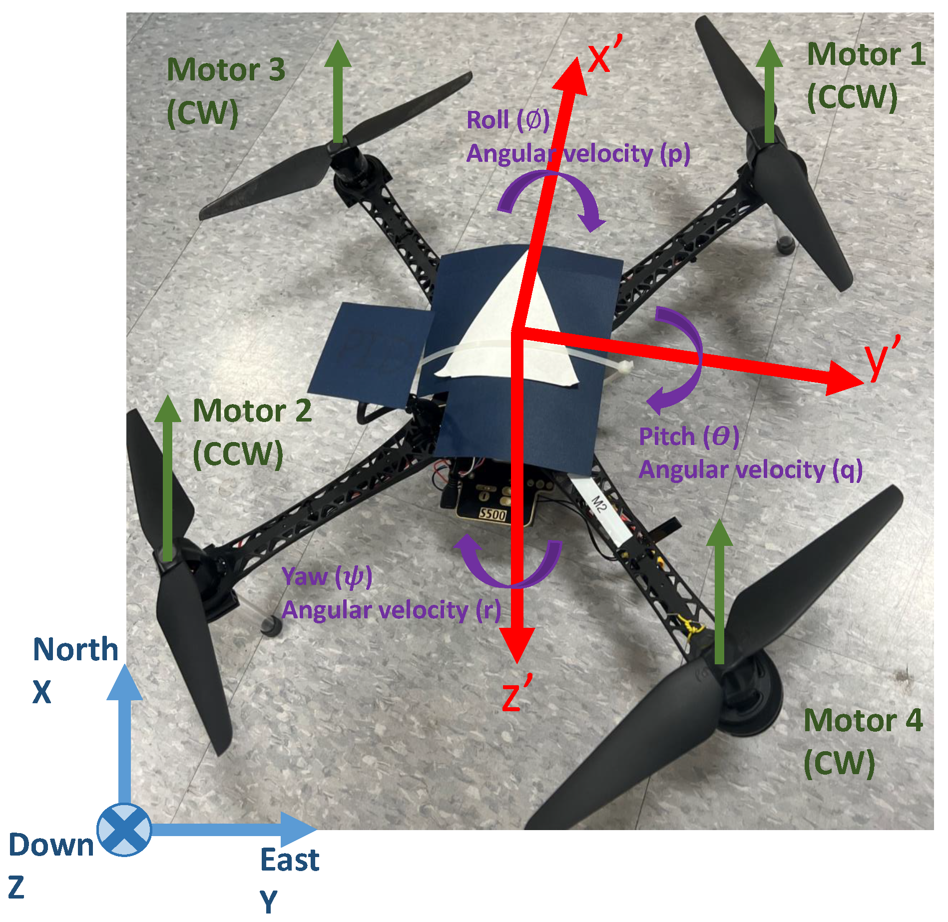
While there are a number of options for control design, one should also consider whether to design attitude controllers based on quaternions (see, e.g., [
29]) or on Euler angles (see, e.g., [
30]). Quaternions are particularly useful for describing rotations in three dimensions [
31], with the main advantage of avoiding the problem of gimbal lock that may otherwise occur with Euler angles when two of the rotation axes align [
32], causing a loss of one degree of freedom. However, Euler angles are more intuitive, representing rotations around the principal axes (X, Y, and Z) or roll, pitch, and yaw, respectively. Most sensors directly provide the measurements in Euler angles, making their integration into control systems straightforward. Moreover, Euler angles can be more computationally efficient in certain situations [
32]. Quaternion-based controllers are not short of advantages; for example, previous work demonstrates their promise in situations where aggressive drone maneuvers might be preferred [
33], including experimental results [
34] and combining them with SMC [
35]. Given the importance of continuity from our previous work [
26], we utilize here the SMC controller from the cited study with Euler angles.
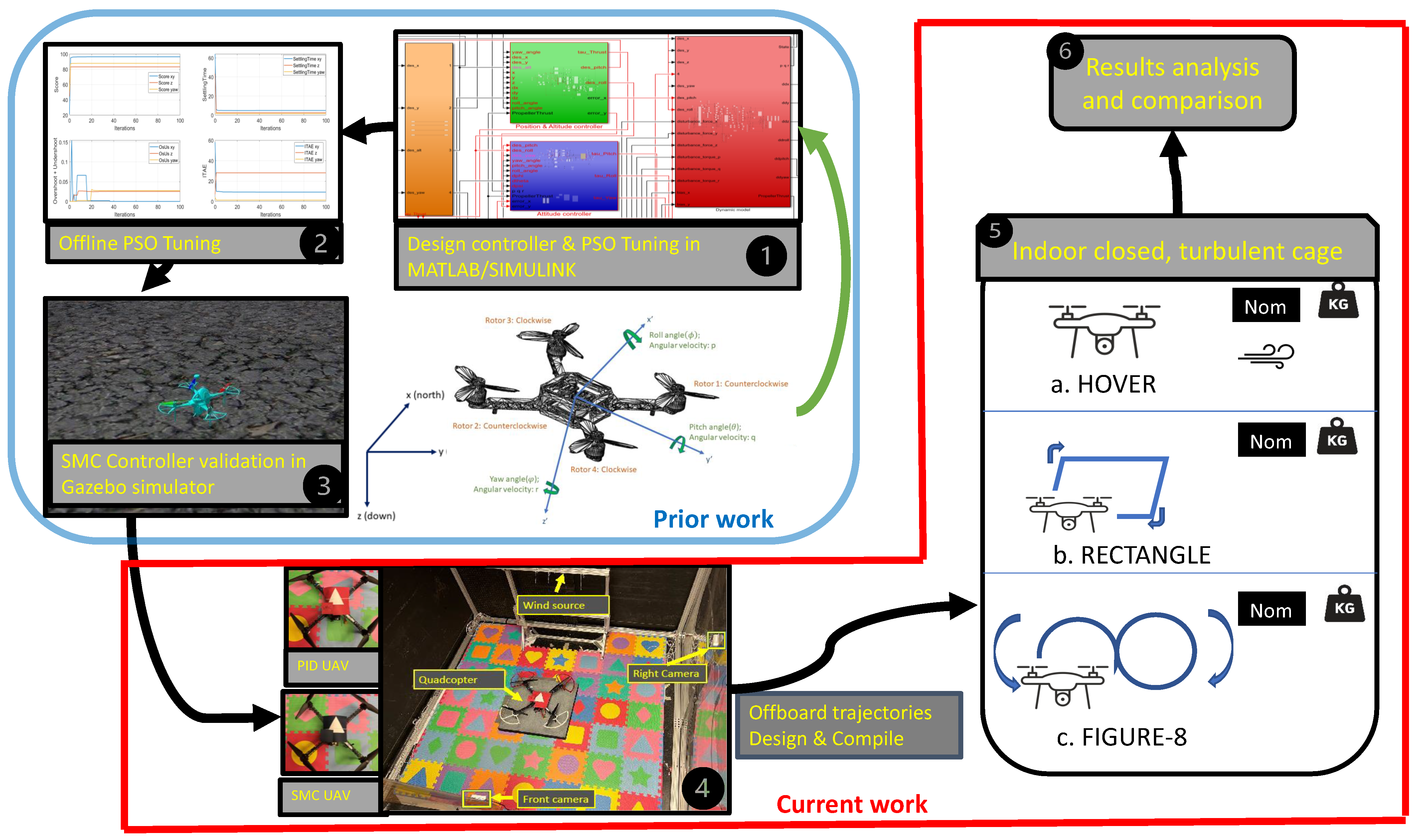
Based on our previous research [
26] regarding a PSO-optimized SMC with disturbance observers (
Figure 1: phases (1) to (3)), we have already developed the control theory and validated the controller using a simulated PX4-conducted (an open-source autopilot) quadcopter. To summarize the work, we firstly designed the SMC controllers as well as corresponding disturbance observers in MATLAB/SIMULINK for the theory validation and then optimized SMC parameters using an offline PSO method. We also built a PX4-conducted quadcopter simulator to validate the optimized SMC. In simulations, we compared this SMC with several PSO-optimized PID controllers and showed its superiority. The PSO-optimized SMC with disturbance observers facilitated more accurate and faster UAV adaptation against disturbances in the environment.
To further validate our proposed SMC controller, in this work, we designed a series of indoor experiments for an actual quadcopter as shown in
Figure 1 phases (4) to (6). In order to be compatible with the actual UAV as well as its autopilot, we upgraded the proposed control theory, improved the initialization and tuning of the PSO algorithm, optimized the control signal mixing algorithm, and tested the fine-tuned SMC parameters. Unlike most of the current theoretical research, here we validate not only the feasibility and stability of SMC through nominal flights but also the reliability of SMC against dynamic disturbances. These disturbances are designed as a series of imbalanced force/torque loads and turbulence in narrow and closed spaces as shown in
Figure 2. These disturbances were applied to the UAV to mimic the most likely future indoor scenarios and to evaluate how well SMC performs.
To the best of our knowledge, most studies on SMC rely on computer simulations and remain in the theoretical phase [
36,
37,
38,
39,
40,
41,
42,
43], while implementation of SMC on actual quadcopters is rare and limited [
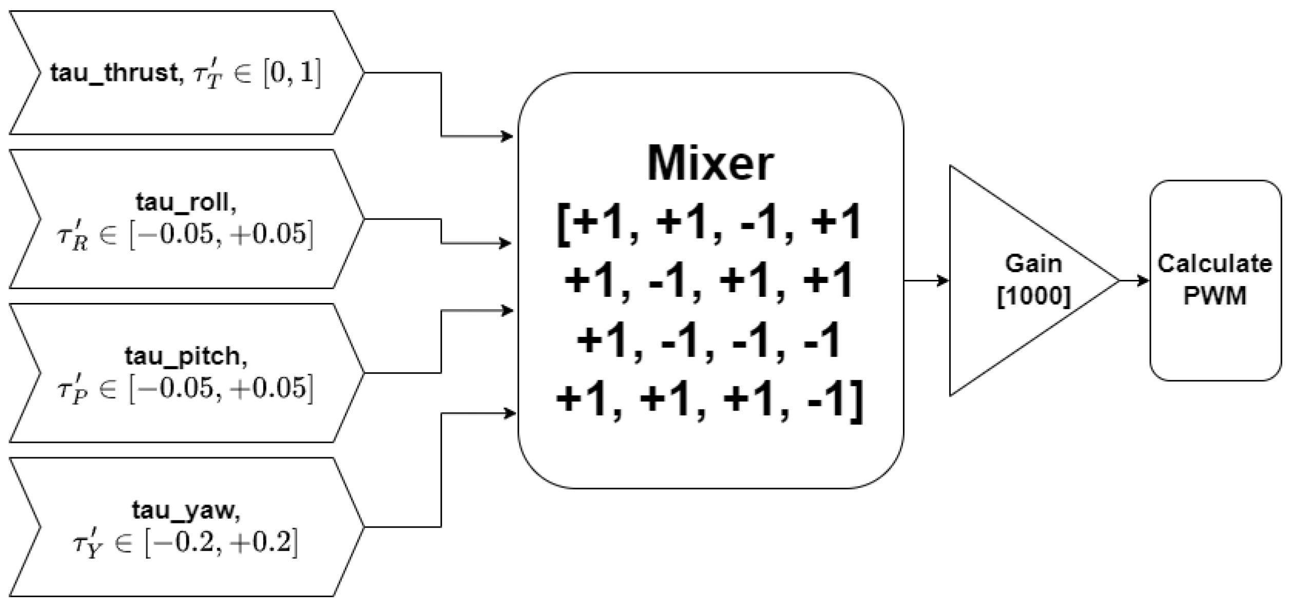
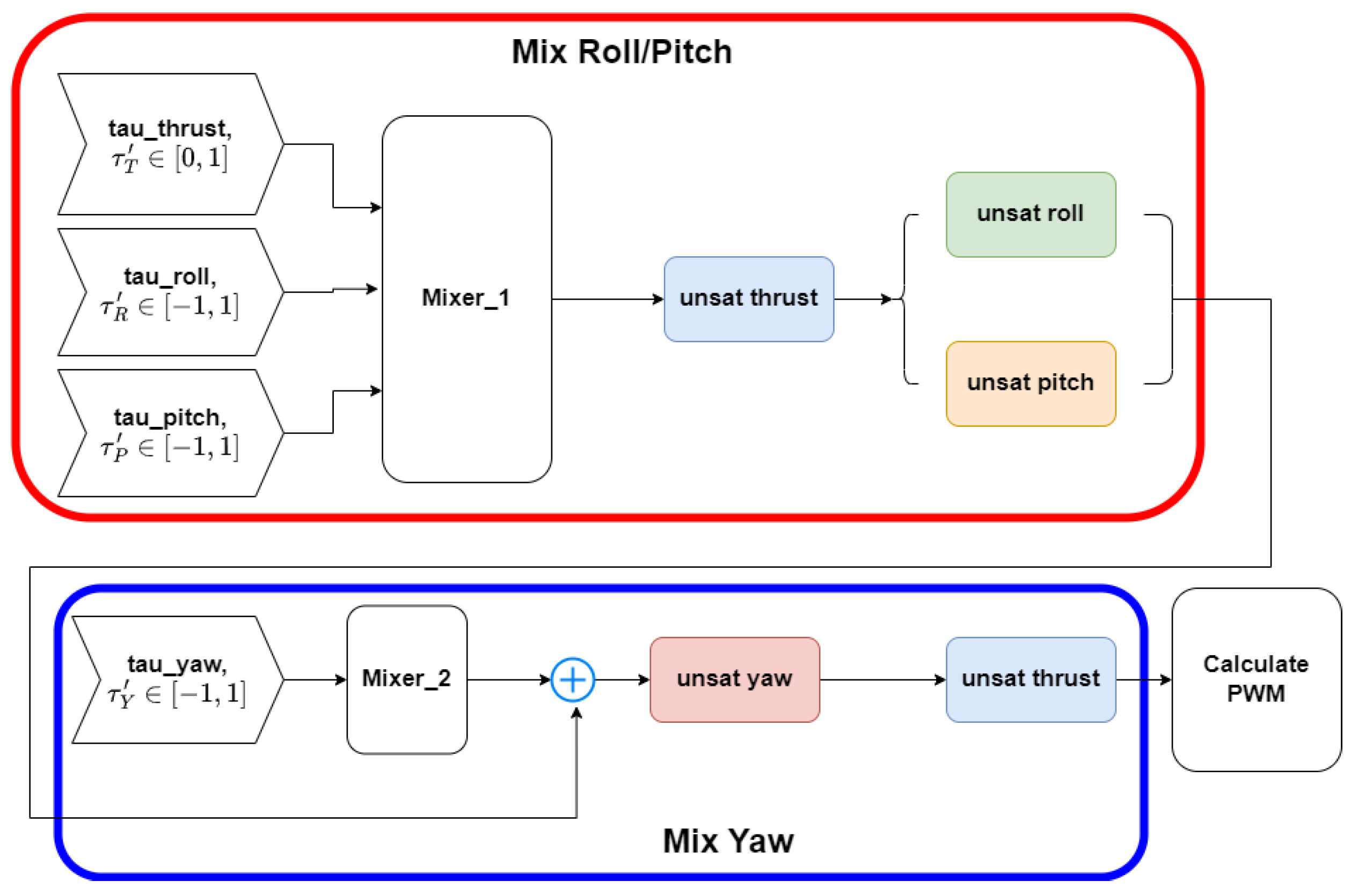
44], let alone extensive experiments in extreme environments. This is likely because the hardware implementation is quite involved and bridging theory with practice is not straightforward. First, the frequency of the control signal must not be too low to ensure the stability of the control, so the signal synchronization process becomes important. In this study, we use the PX4 open-source autopilot, which provides fixed-rate and continuous feedback of sensor signals and actuator signal outputs. However, due to hardware limitations, the control frequency cannot be too high, so the controller frequency and the fundamental sampling frequency are fixed at 250 Hz. Second, we need to filter sensor data within a reasonable bandwidth due to unavoidable sensor uncertainties, such as noise and signal gaps. Here, we use an extended Kalman filter (EKF) estimator with a cutoff frequency of 30 Hz for the IMU/GYRO sensor to reduce computational consumption and UAV vibration. Third, due to the delay and response time of the actuator, which can be negligible in simulations but critical when dealing with real UAVs, we choose a reasonable PWM update rate, which is 400 Hz, based on the type of motors utilized. At the same time, the mixing process of the actuator signals is unavoidable for the hardware implementation, without which the PWM signals can easily exceed or fall below the physical limit values, causing instability. This can be also an issue for the sensitivity of disturbance observers, which estimate dynamic disturbances and feedback these estimates to the main control loop for disturbance rejection. Therefore, including a reasonable control signal mixing is critical to ensure the aerial stability of the UAV in the real world. Fourth, the PSO algorithm is not implemented in real time because of its high computation cost and time-consuming process. Instead, the PSO tuning results are based on a purely mathematical model and take into account the theoretical stability of the SMC. In more detail, the PSO is run and iterated in conjunction with SIMULINK, after which we encode and embed PSO-tuned parameters onboard the UAV. Note that not all PSO-tuned parameters are applicable to an actual UAV; thus, a further manual tuning process is required. We modify the parameters judiciously via an initial calibration phase first, according to different orientations (pitch, roll, and yaw) and different directions (
X,
Y, and
Z) of the quadcopter. Although we have simultaneously developed an in-flight remote SMC parameter adjustment system that relies on a lightweight wireless communication protocol called MAVLink, we do not recommend adjusting parameters in-flight because of the possibility of improper adjustment leading to an accidental crash. Instead, we start a brand new flight after the hardware coding and updating of each parameter and finally evaluate the flight performance in terms of settling time, overshoot, and rise time based on the flight log data. Finally, after each iteration of parameter tuning or controller modification, we use the MATLAB code generator to automatically generate the C code and upload the new firmware to the actual UAV microcontroller board.
In view of the above discussions, the novelty of our work can be summarized as follows: We first demonstrate what additional steps are needed when transitioning from [
26] the particle swarm optimization (PSO)-tuned sliding mode control (SMC) with a disturbance observer (DOB) to real-time control, hardware implementation, and experiments. This is a topic of strong interest but with little guidance in the open literature. Next, we demonstrate how the drone performs at the face of a set of complex disturbances, such as wind and unbalanced weights under SMC, and in particular show how a combination of these disturbances can still be addressed by SMC—an experimental condition that does not exist in the literature to the best of our knowledge. Furthermore, we complement the SMC experiments with those by PID controllers as industry-standard benchmarks, for comparisons with respect to SMC. Lastly, with the use of the DOB, we demonstrate how to estimate wind direction and wind forces in real time—a critical capability in monitoring the environment and atmospheric conditions. These results add to the body of literature rapidly growing and will help support future research into the robust control of drones in challenging environments.
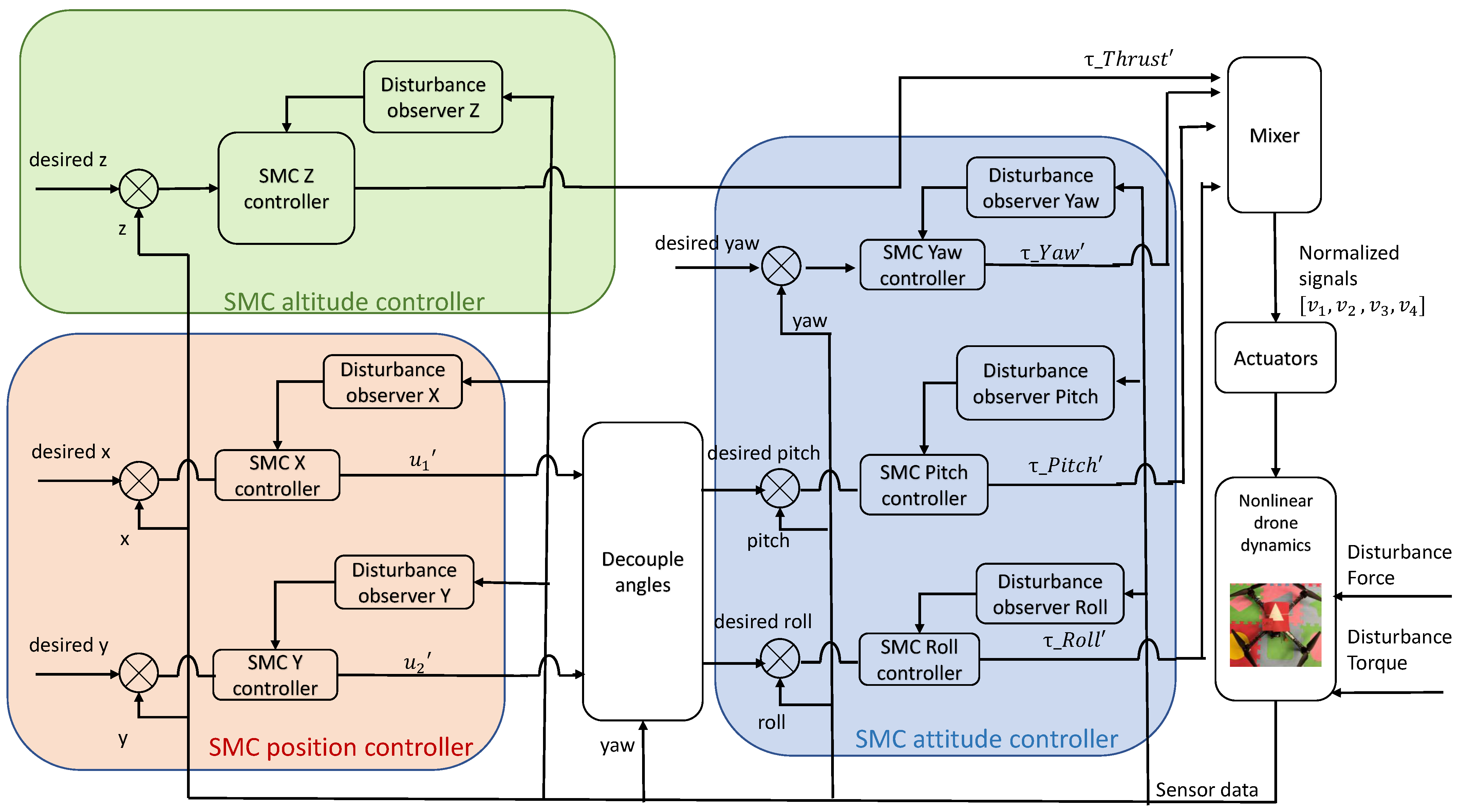
In the next section, the system is defined and the equations of motion for the quadcopter are summarized. In
Section 3, the SMC control laws are developed for the attitude and position dynamics, a disturbance observer is designed, improvements in the control signal mixing process are explained, and the tuning process on the physical UAV is outlined. Next, in
Section 4, the experimental setup is described, the step response of the SMC is evaluated, and the trajectory following capabilities of the SMC are compared to a commercial PID controller. Each controller is subject to a variety of disturbance conditions in a narrow, closed, and turbulent chamber.
4. Experimental Results
4.1. Experimental Setup
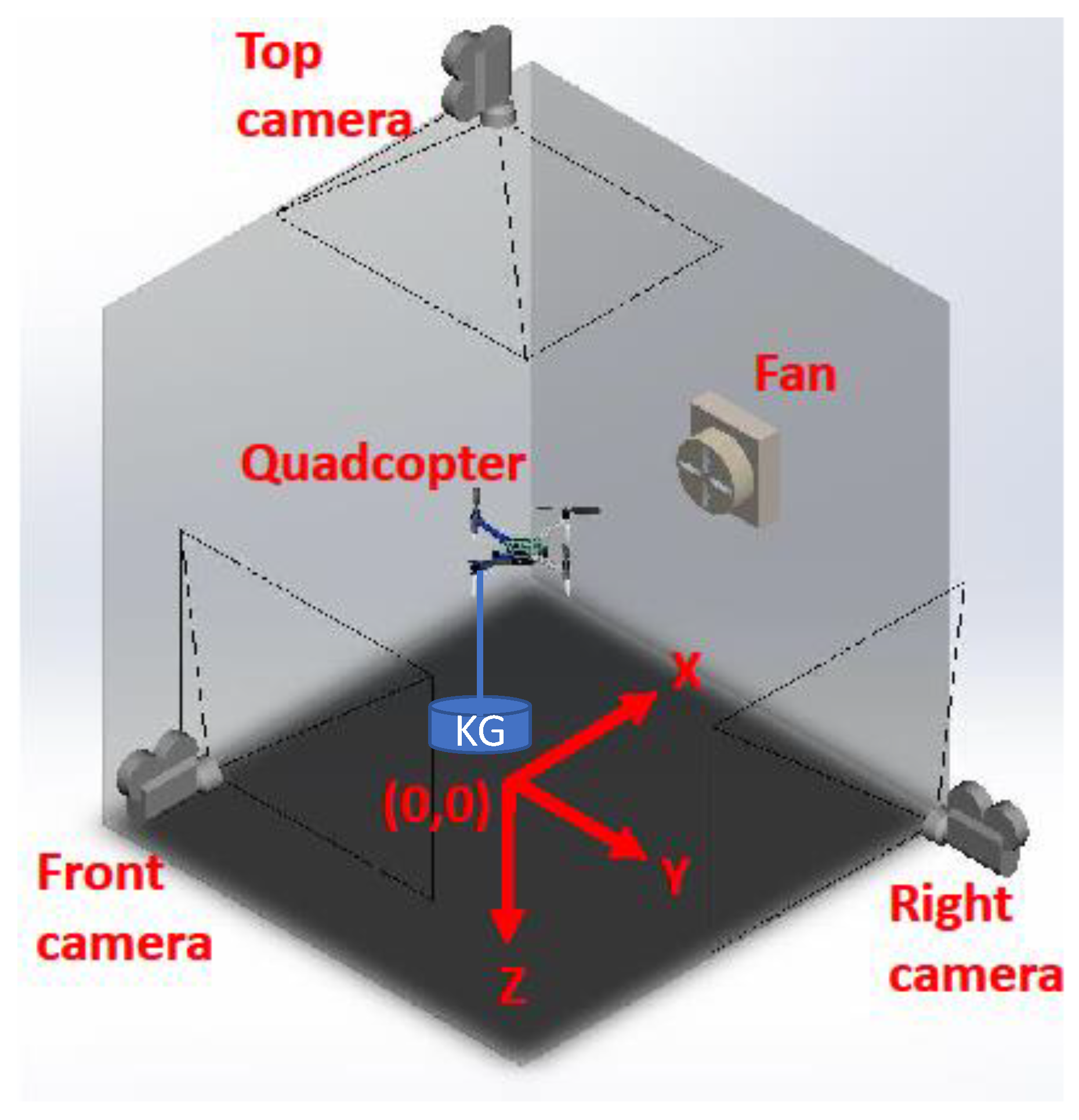
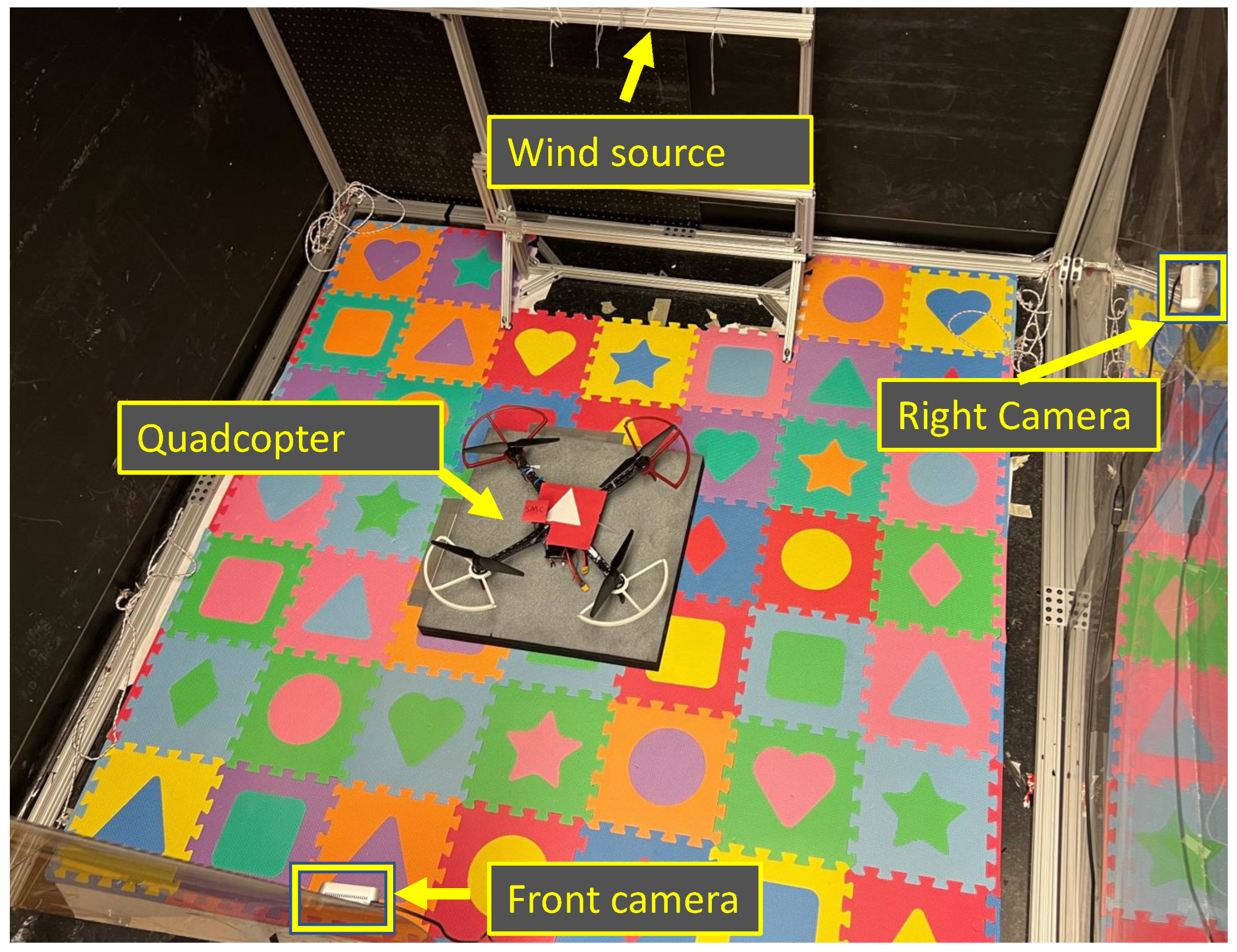
The experiments were conducted in a narrow, closed, and turbulent space, as shown in
Figure 2 and
Figure 10. The testing field was built out of transparent acrylic sheets. The chamber had a length of 2.15 m, width of 2.20 m, and height of 2.30 m. Three cameras were located along each of the NED axes. The stationary wind source (location marked in
Figure 10) was turned on before the flight and turned off after the flight. The thrust produced by the fan could be adjusted by a remote controller (RC). Rag strips were attached around the edges of the wind source in order to illustrate the wind. The indoor navigation was achieved by the onboard realistic states measurement system consisting of a visual inertial odometry (VIO) system and three redundant inertial measurement units (IMU). In addition, to validate the data from the onboard sensors, the position and trajectory of the UAV was also recorded by three external, fixed high-resolution depth cameras.
As the UAV changes its attitude frequently during the flight, winds with dynamic amplitude and changing direction generated by UAV motors combined with a stationary wind source tend to create turbulent airflow in a small, enclosed room. The inertial wind forces dominate over the viscous forces, especially at relatively low altitudes (under 1 m) or near the walls. Based on our measurements, the ratio of the length of the UAV to the length of the cage is around , which means even when the UAV is located at the center it is still easily affected by the airflow near the walls.
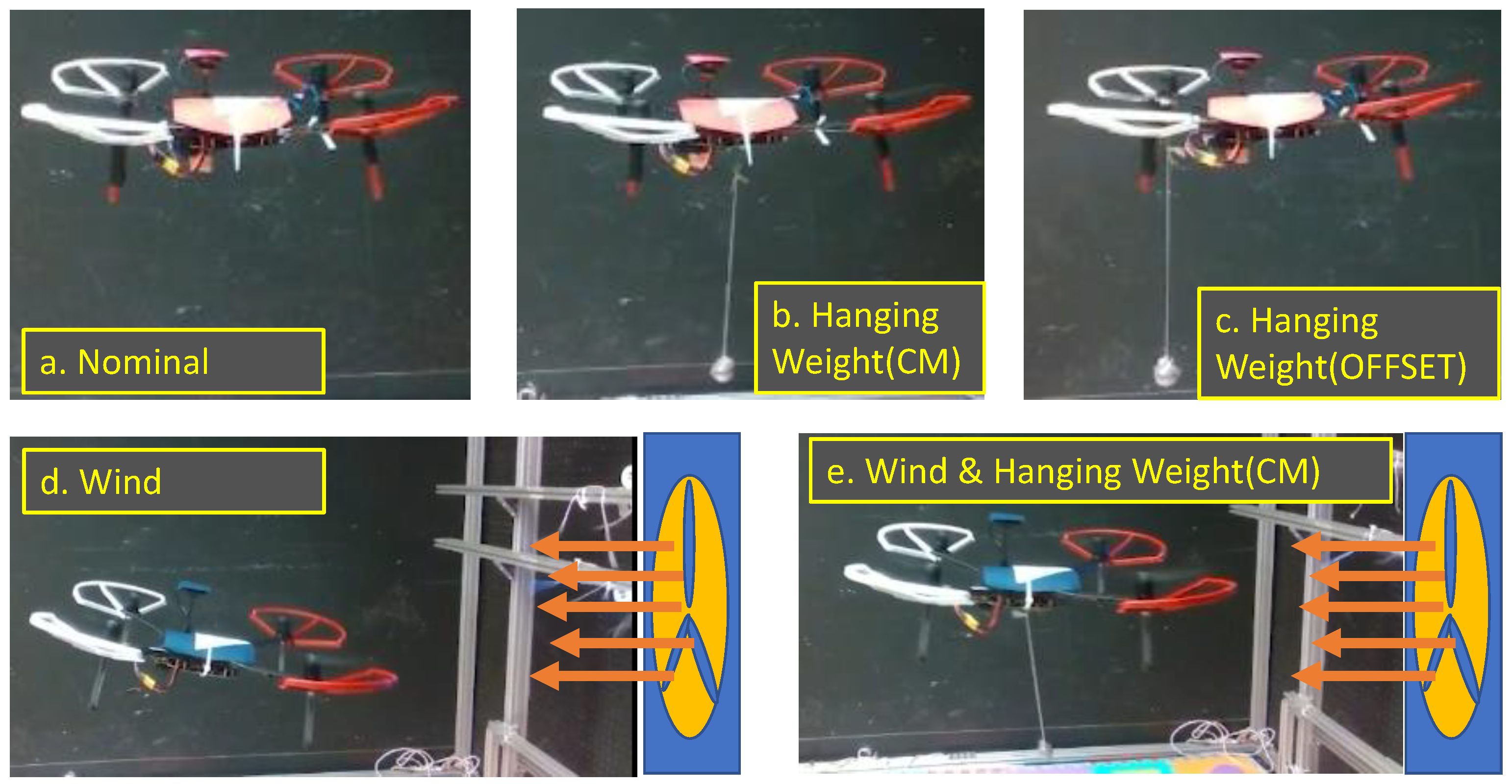
Five representative cases of experiments were designed, as shown in
Figure 11. The first case was nominal flight without intentionally added disturbances, which means the disturbances perceived by the flight controller were mainly induced by the UAV itself (physical characteristics) as well as the diffused turbulent airflow within the small testing field, for example, the imbalance caused by varying battery positions, sensor distribution, the vibration from the actuators, and the changing turbulent flow, which depends on the UAV’s position and speed. The second scenario was flying with a suspended spherical weight that was attached at the center of mass (CM) of the UAV. The length of the string was 0.35 m and its weight was negligible, and the mass of the metal ball was 131.7 g. As shown in
Figure 11b, when flying, disturbance force would be decomposed into
X–
Y–
Z directions and the force magnitude in each axis could change due to the back and forth swinging of the metal ball. The third scenario, which is shown in
Figure 11c, was similar to the second case except the suspended weight was attached to the end of the right-rear landing gear; thus, this time not only were dynamic disturbance forces in
X–
Y–
Z induced, but also variable disturbance torques in pitch roll and yaw were generated.
Due to the uncertainty of the real-world environment, such as unpredictable wind gusts, variable weather conditions, and so on, a series of comprehensive wind experiments are necessary in developing a new, reliable, robust flight controller, as shown in
Figure 11d,e. The fourth scenario was to hold the position under a unidirectional wind. This was also regarded as the wind-only case since no extra disturbance was added except the wind. From the 3D environment diagram in
Figure 2, the wind was produced directly in front of the UAV. The maximum wind speed at the position of the UAV was 9 m/s. Since the wind tends to spread and disperse over a range, the effective distance of the lateral wind would be limited, and the magnitude and direction of the wind depends on the flight position of the UAV. The fifth case of experiments, shown on the bottom-right of
Figure 11e, was an extension of the wind-only experiment, and the UAV was loaded with a spherical suspended weight.
4.2. SMC Performance Analysis
The SMC was subject to step inputs in the
X,
Y,
Z, and
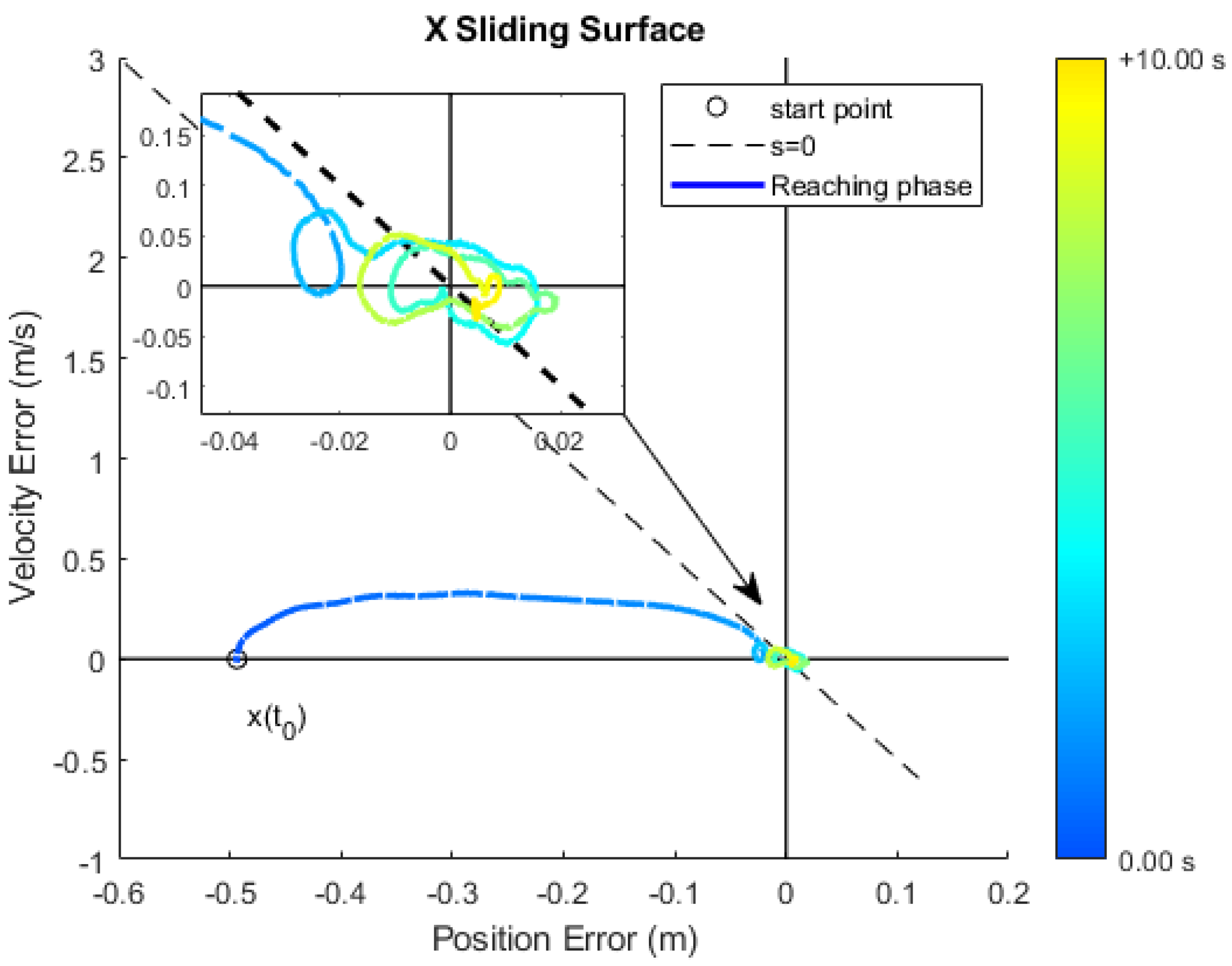
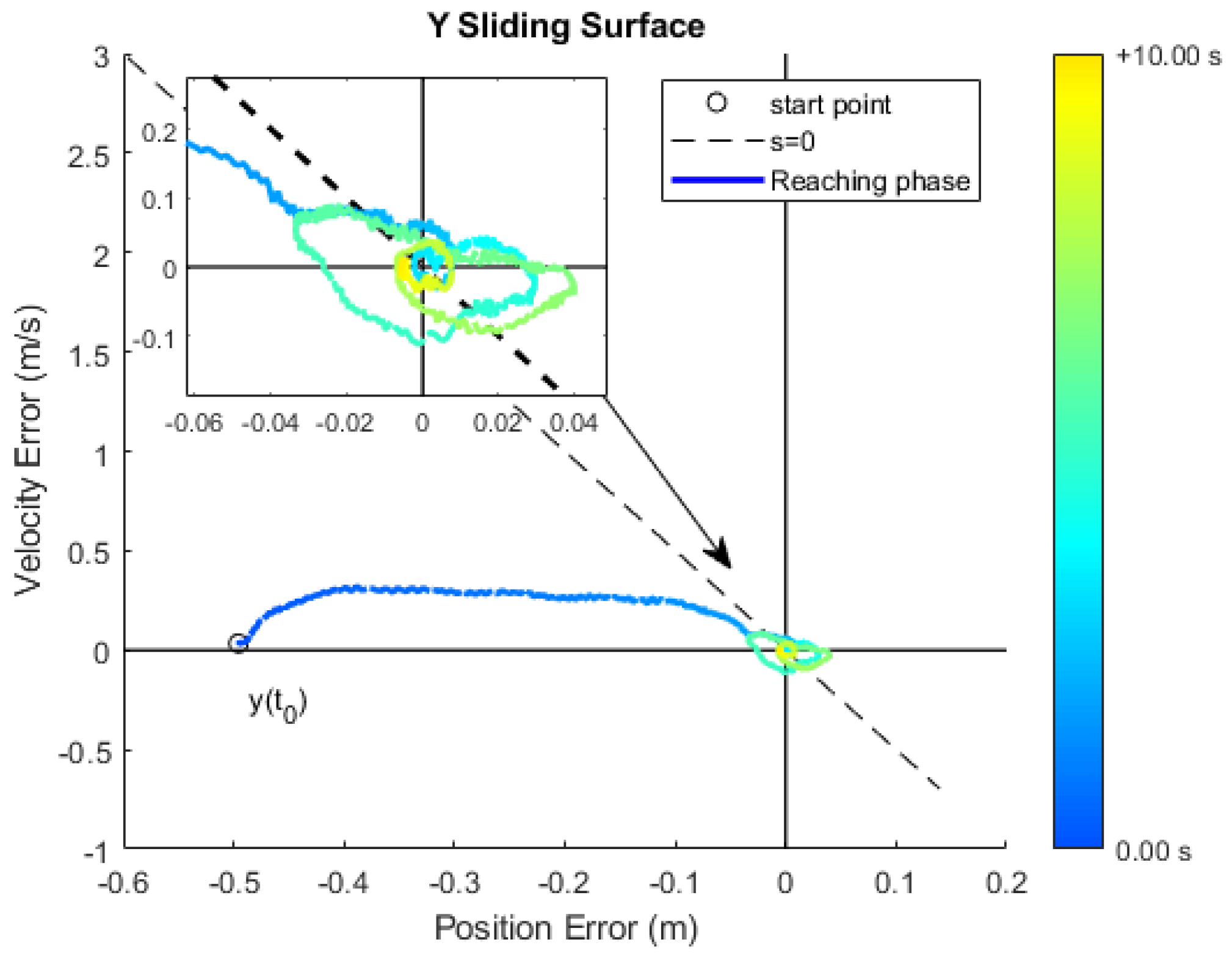
axes in four separate experiments to evaluate the error dynamics of the controller. Plots of the velocity error
against the position error
e with the s = 0 hypersurface included on the graph are described throughout this section. In the
X axis, a step input of 0.5 m was applied. The response can be seen in
Figure 12.
The error exhibits both the reaching and sliding phases, as expected. In the reaching phase, the velocity only reaches 0.5 m/s, producing a flat reaching mode response, and the sliding mode is achieved as the controller drives the error to 0 (see
Figure 12). The
Y axis was also subject to a 0.5 m step input. The error dynamics performed very similarly to the
X controller, as shown in
Figure 13. The slow reaching mode dynamics of the
X and
Y controllers is because of the nested-loop controller structure. That is, the
X and
Y responses are subject to the pitch and roll dynamics.
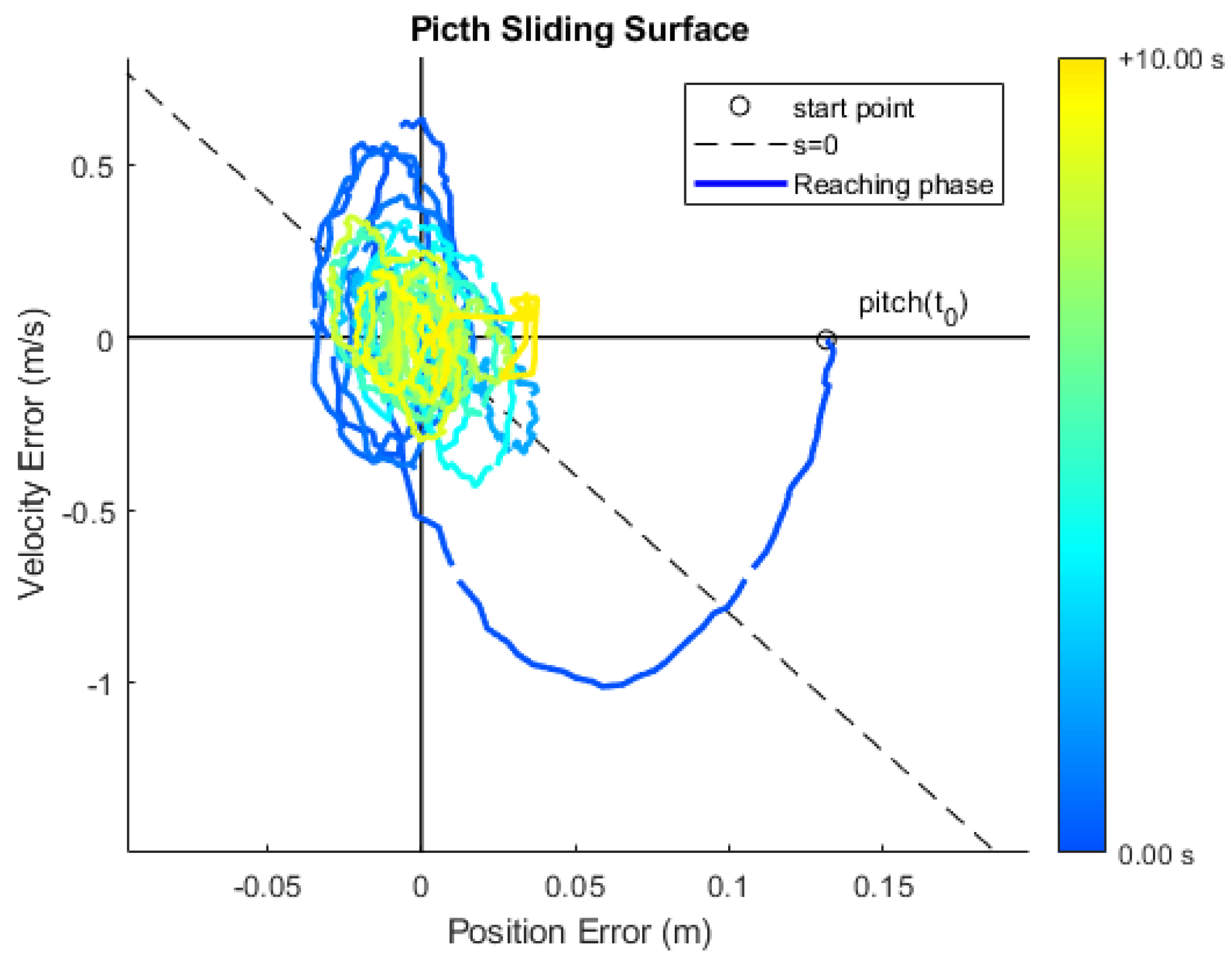
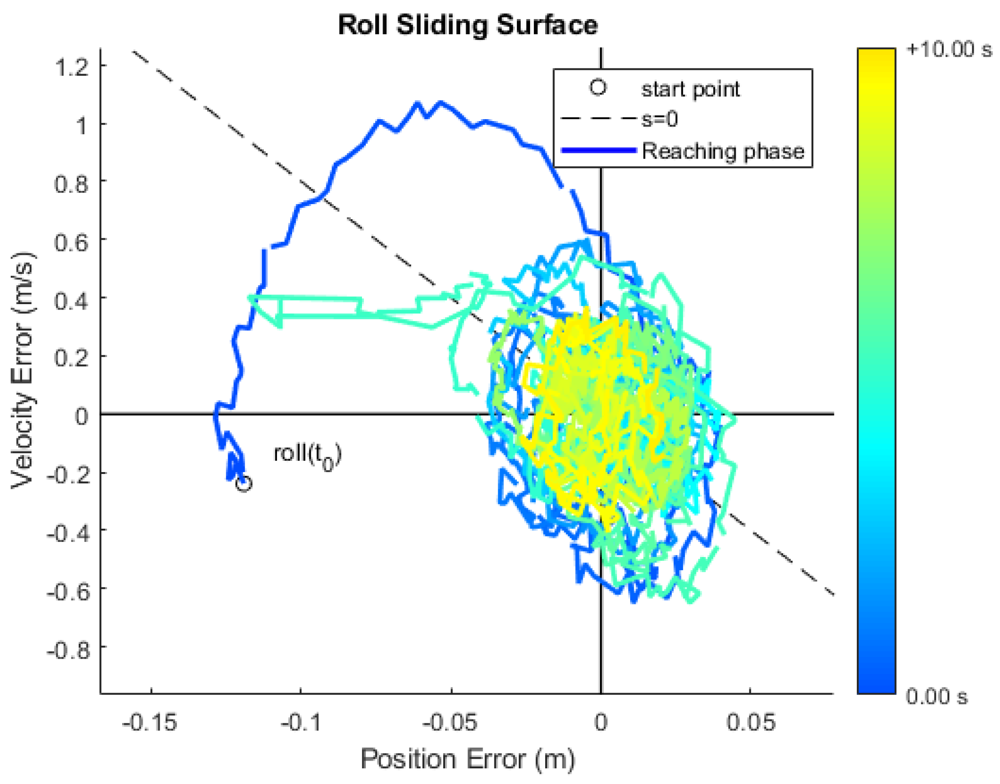
Figure 14 and
Figure 15 show the pitch and roll sliding modes during the respective
X and
Y step inputs. The pitch and roll error dynamics very quickly pass through the reaching mode and enter the sliding mode, which is what causes the flat reaching mode curves in
X and
Y.
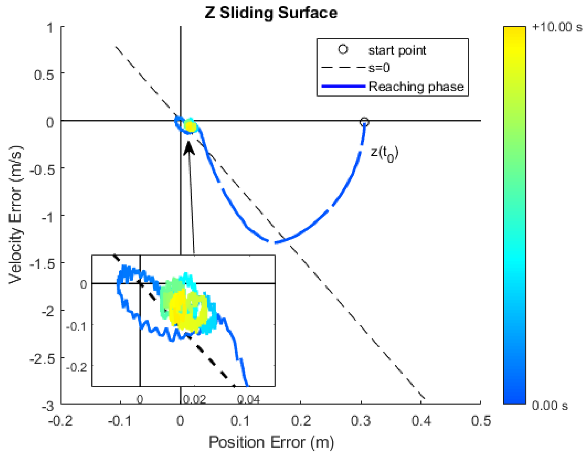
The
Z axis was subject to a 0.3 m altitude step input. As shown in
Figure 16, the reaching mode overshoots the sliding surface but then smoothly re-approaches it while entering the sliding mode. This relatively smooth oscillation about the sliding surface is allowed by the saturation function. If the saturation function were not used, the sliding mode would be achieved faster, but there would almost certainly be chatter about the sliding surface at the transition from the reaching mode to the sliding mode.
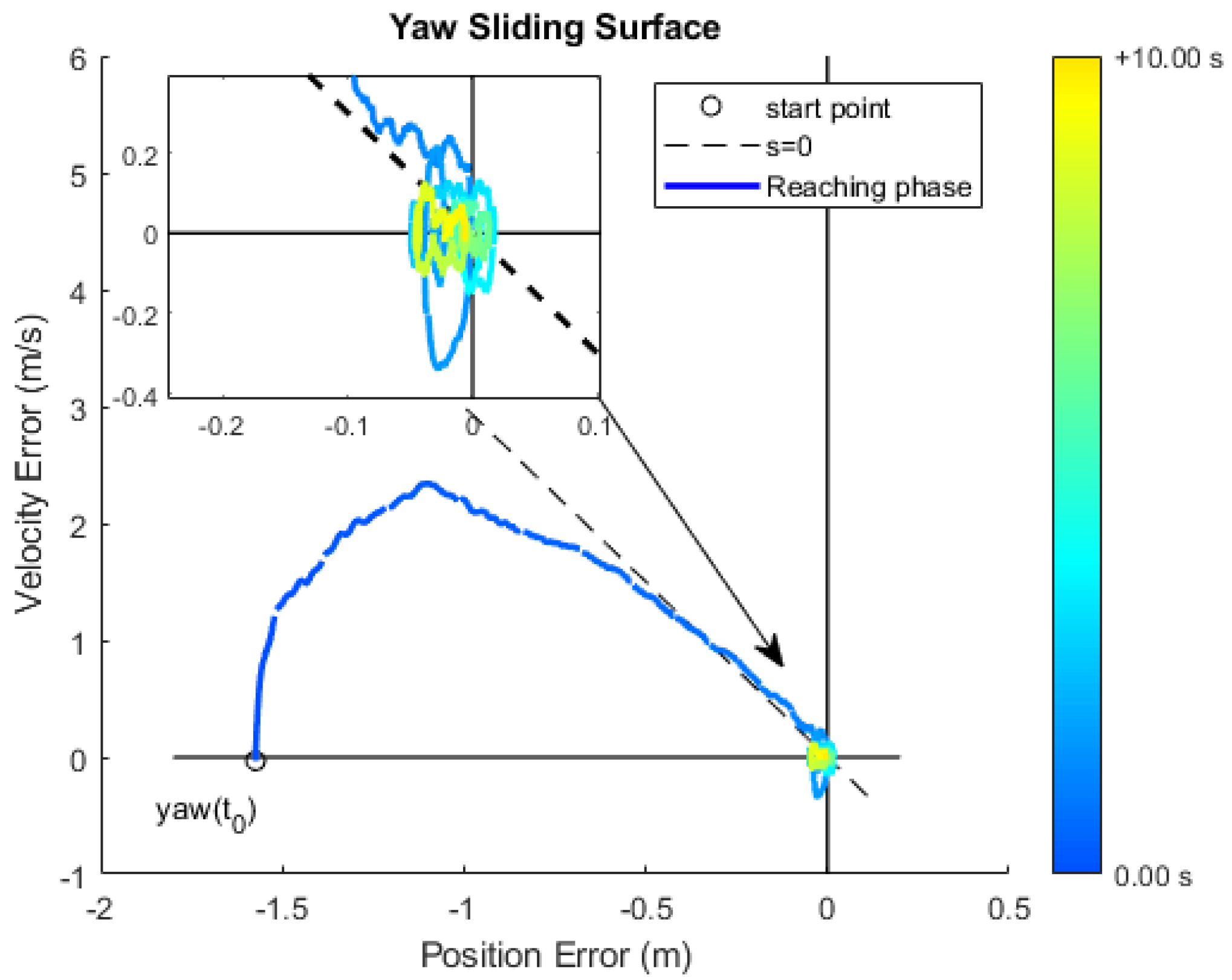
Finally, the yaw was subject to a 90 degrees clockwise step rotation (
Figure 17). Similarly to the
Z error dynamics, without the saturation function the transition from reaching mode to sliding mode would occur sooner. Instead, there is some undershoot of the sliding surface initially, then a smooth convergence towards the sliding surface. The yaw motion here may be a bit conservative, but due to the coupling of the attitude dynamics, this is required for a smooth system response. More aggressive yaw control introduces chatter into all of the attitude control variable outputs, which propagates through the system.
All of the axes subject to step inputs following the conventional reaching mode to sliding mode error dynamics, as expected. The X and Y response is limited by the attitude dynamics. The Z controller overshoots the sliding surface slightly when reaching the sliding mode, while the yaw controller undershoots the sliding surface. The overshoot and undershoot of the sliding surface are allowed by the use of the saturation functions on the switching portion of the control law, instead of a more aggressive sign function.
4.3. Trajectory Tracking
The tracking performance of the SMC was tested on three different trajectories: hovering, a rectangle, and a figure eight. In each trajectory, the UAV ascended to an altitude of 1 m at 0.1 m/s then performed the desired trajectory and returned to the ground at 0.1 m/s.
For the hovering trajectory, the setpoint (0 cm, 0 cm, 100 cm, 0 deg), in X, Y, Z, and was sent to the UAV for the entirety of the trajectory.
The rectangle was comprised of four sides with a length of 30 cm, which were traversed in 3 s each. There was a 1 s hover at each corner of the rectangle. Yaw of 0 degrees was maintained throughout the trajectory. The pattern was repeated twice before landing.
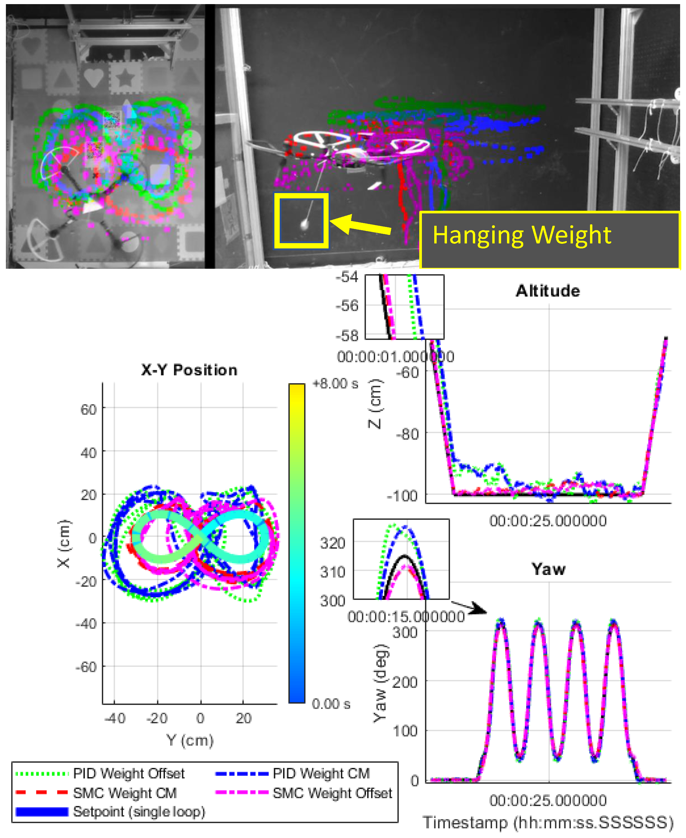
The figure-eight pattern had a radius of 30 cm and the UAV was commanded to face in the direction of travel for the entirety of the trajectory. A total of four loops of the figure eight, each 8 s in duration, were completed prior to landing.
Each of the trajectories was completed with no disturbance applied to the UAV (the nominal case); with a weight hanging from the center of mass of the UAV (weight CM case); and with a hanging weight offset under one of the motors (weight offset case). In addition to these disturbances, for the hover trajectory, the UAV was subject to a wind disturbance along the axis. This wind disturbance was applied with no weight added to the UAV (wind case) and with the hanging weight at the center of mass (wind and weight case).
The results are organized by trajectories through the remainder of this subsection in the following order: hover, rectangle, figure eight. The primary quantitative metric for comparing the performance of the controllers is the root mean square (RMS) error in each axis. The RMS error is reported in centimeters for the translational axes and degrees for the rotational axes.
4.3.1. Hover
The RMS error along each axis for the hover trajectory subject to each of the types of disturbances is summarized in
Table 2. As a general trend, the RMS error increased with each experiment to the right along the table. This suggests that, as intended, the difficulty of the control problem increased as more severe disturbances were added.
In the nominal case, the SMC had an over 2× reduction in RMS error compared to the PID for X and Y tracking. That improvement increased up to a 5–10× error reduction when disturbances, especially wind disturbances, were added. The Z error for the SMC was less than or around 2 cm for all experiments, regardless of the disturbance applied. Conversely, the PID had a Z error larger than 15 cm and a higher tracking delay for all experiments. The graphs of the experiments revealed that there was a steady-state error of 10–20 cm present for all of the PID results. The PID controller was unable to maintain the desired altitude especially under disturbances. The yaw error was 2× better with the SMC and relatively improved when the wind was added. However, the pitch and roll errors were comparable between the two controllers.
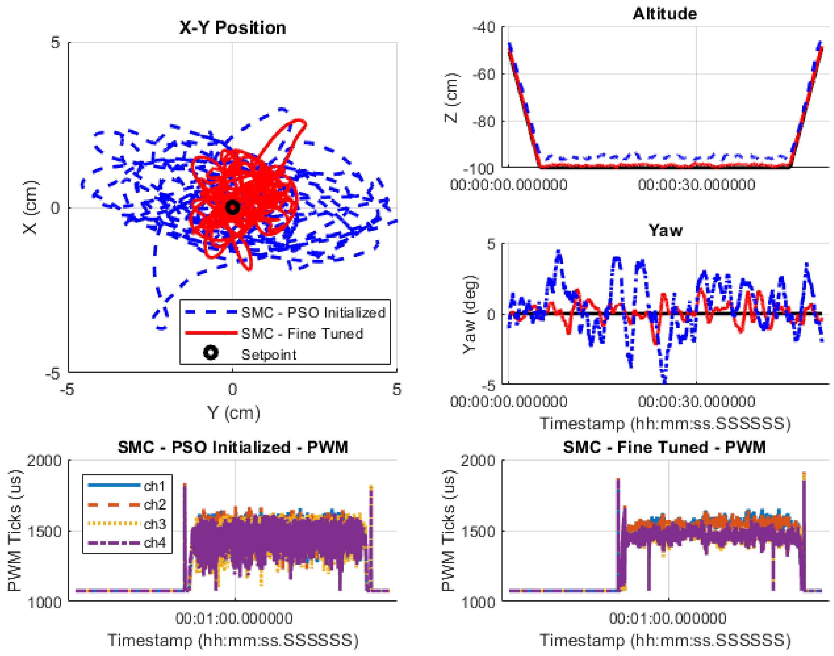
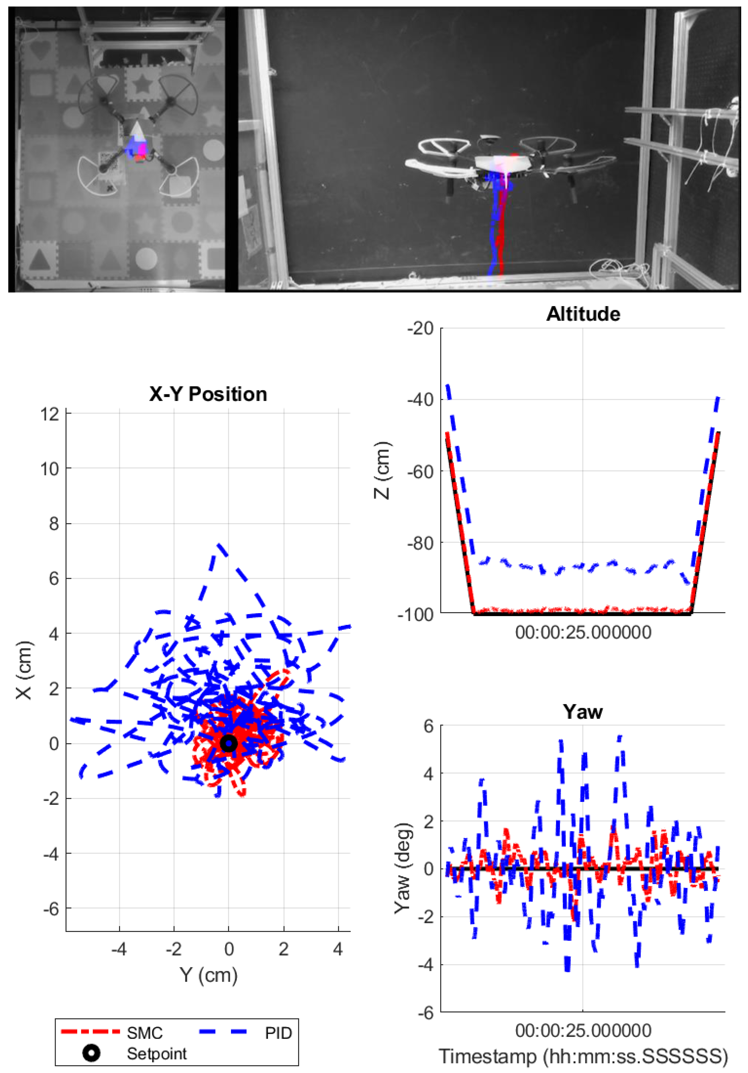
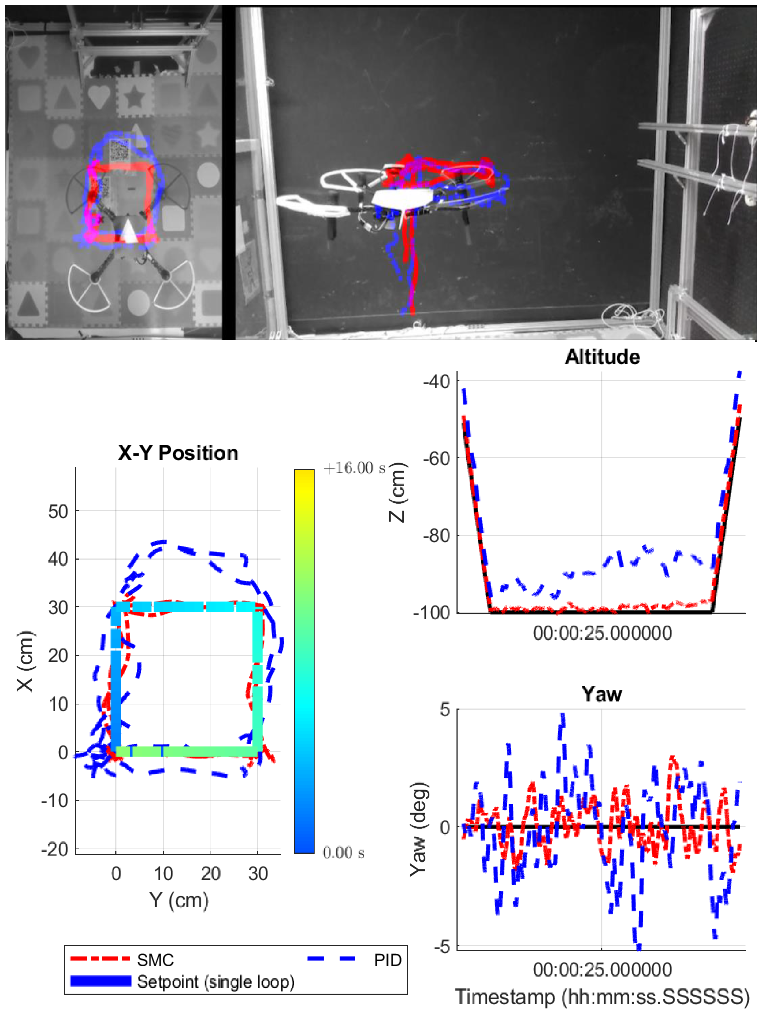
Graphs comparing the
X,
Y,
Z, and heading tracking of the PID and SMC controllers for the nominal case are presented in
Figure 18 based on the flight logs, along with overlays of the trajectories captured by the top and side cameras in top of the figure. Similar results could be obtained from the camera recording images or the onboard flight logs that the drift area of SMC was significantly smaller than that of PID during hovering. From the sensors’ data, the SMC clearly had less variance in
X,
Y, and yaw than the PID controller. Additionally, there was a steady-state error of over 15 cm for the PID controller in the
Z axis. Similar trends can be seen in
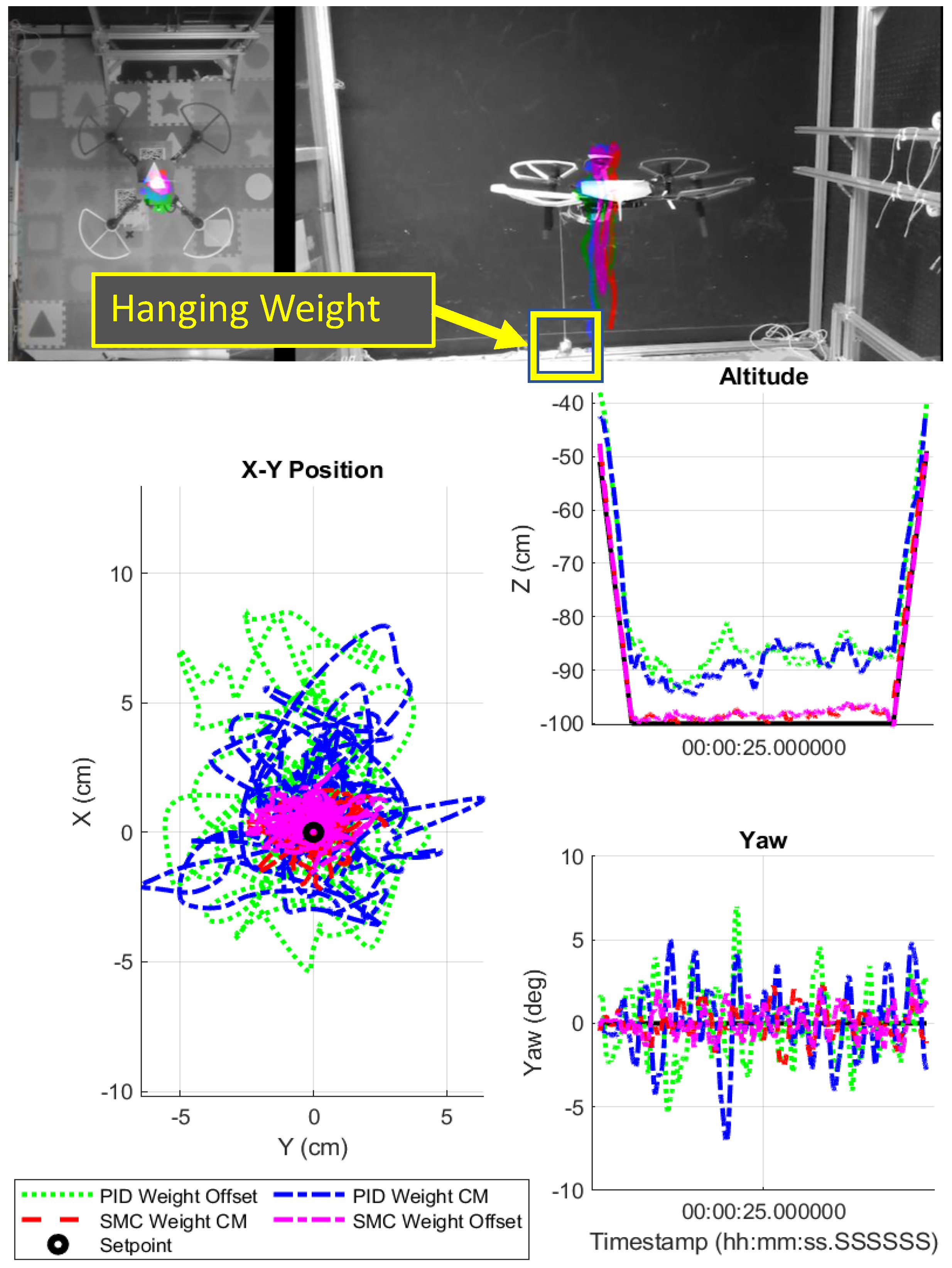
Figure 19 and
Figure 20, when the hanging weights were added. The PID had a larger fluctuation in yaw angle of over 5 degrees, while the SMC fluctuated less than 2 degrees.
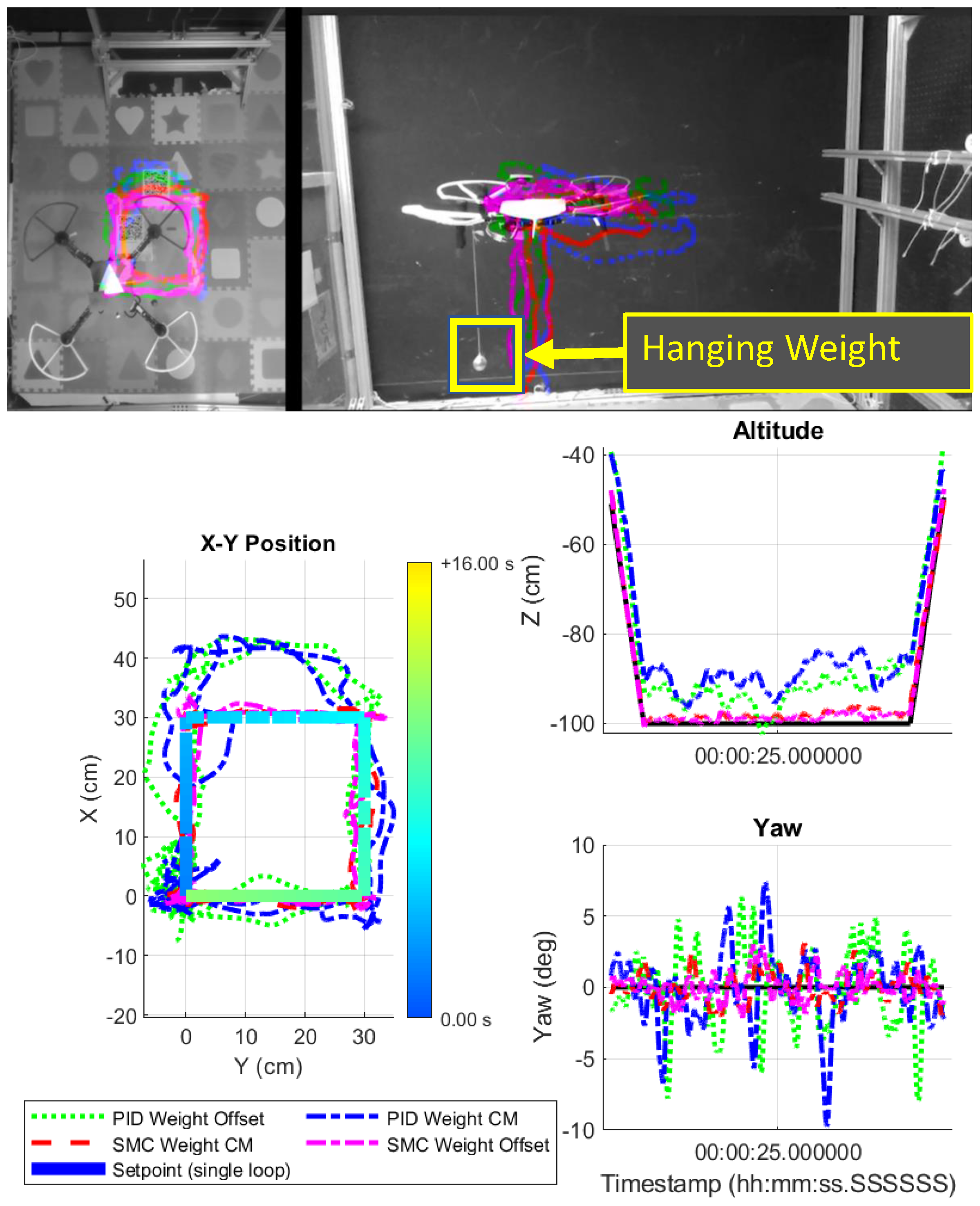
In
Figure 19, hanging weights were attached to the center of mass or to the end of the landing gear. The SMC was able to maintain its setpoints with or without the payloads. In contrast, the PID had a relatively larger position and heading error, and its drift area in the XY plane increased when an offset hanging weight was added. In addition, the suspended payload had a significant effect on the tracking of the PID in the
Z direction. From the results, the PID pulled up and down the UAV when the weights swung from side to side.
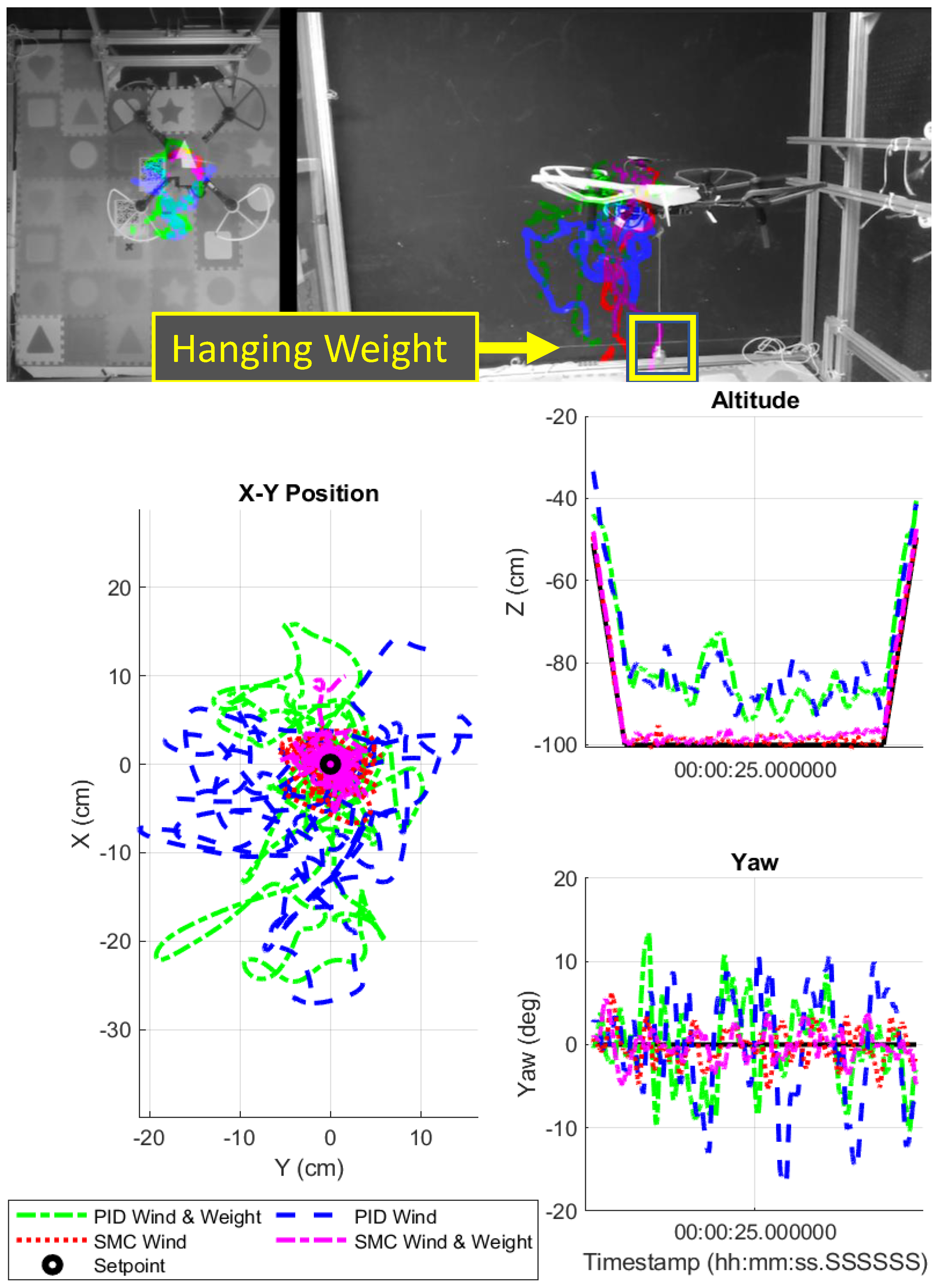
Finally, the plots and overlays for the case when the wind was added are in
Figure 20. The PID was blown in the direction of the wind on several occasions (green and blue), while the SMC was able to resist the wind disturbance and more accurately maintain the setpoint position (red and pink). There was an oscillation in the
Z axis of the PID-controlled UAV caused by it being pushed up and down in the wind. Furthermore, the SMC-controlled UAV fluctuated less than the PID-controlled UAV in terms of heading.
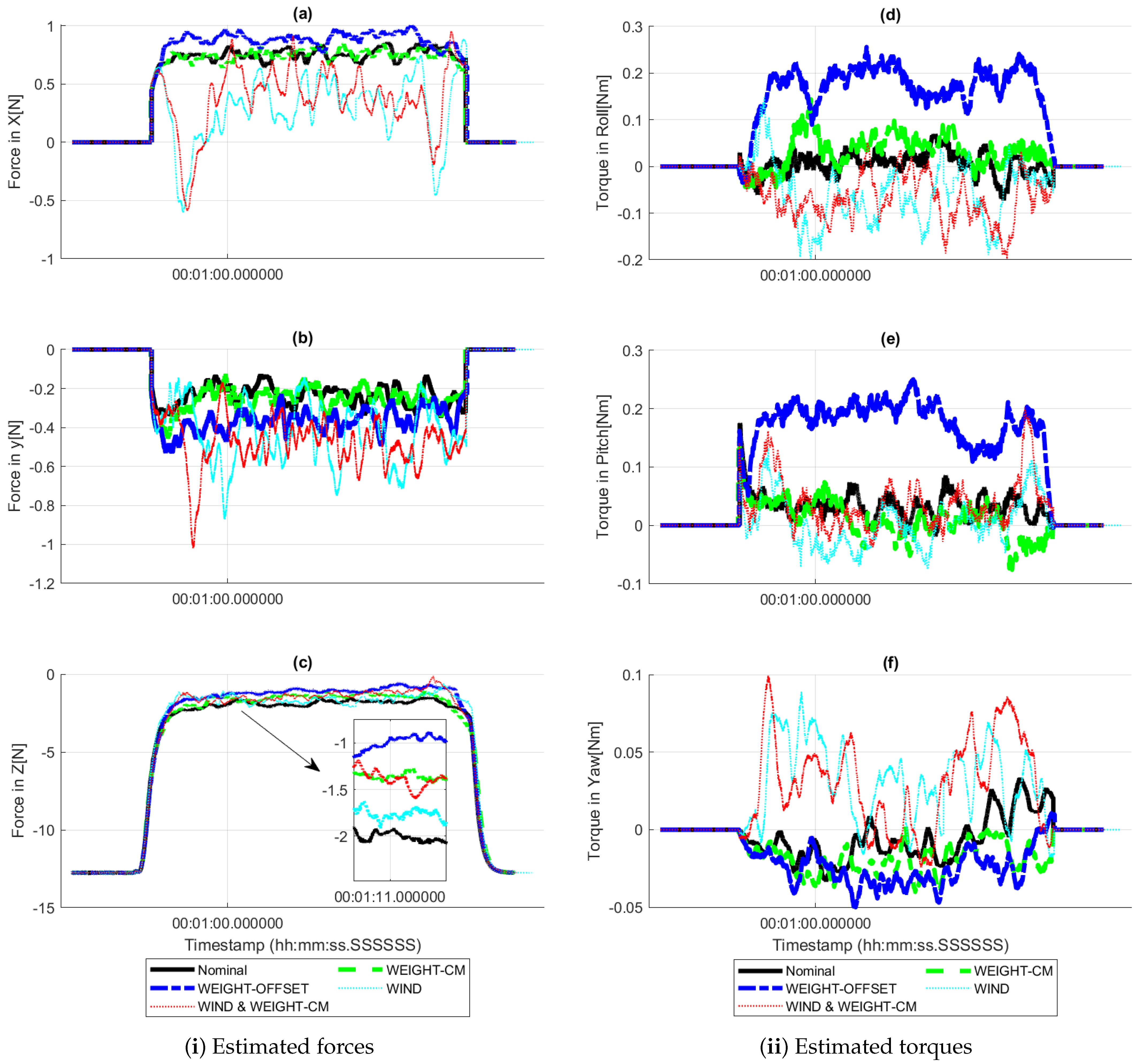
When hovering, the UAV should maintain its current position, heading, and altitude, and it was designed to actively reject any externally applied disturbances, such as forces and torques, with the help of the omnidirectional disturbance observers. In the nominal case,
Figure 21i shows nonzero disturbances of
N in the
X direction,
N in the
Y direction, and
N in the
Z direction, which remained constant throughout the experiment. These baseline disturbances might be caused by small space turbulence, i.e., airflow synthesized from forward, leftward, and downward winds. In other words, ideally, these values should be 0 N if the UAV was located in a large open and undisturbed space. When the UAV was on the ground, as shown in the beginning of experiments in
Figure 21i(c), the force in the
Z direction shows the same magnitude as the UAV’s weight of
N but in the opposite direction, which indicated a disarmed status without any propeller speed.
The force disturbances in the hanging weight cases should have no difference from the nominal case except an additional downward force in the Z direction. By analyzing the average differences between the nominal and weighted cases, we can estimate the weight of the payload to be ≈1 N, while the actual weight of the payload was 131.5 g ( N). When the hanging weight was mounted on the left-rear leg of the UAV, i.e., the weight-offset case in the figure, the observer-estimated forces increased due to the additional thrust produced to balance the torque.
Finally, the magnitude of forces increased significantly in -
X and -
Y after applying the lateral wind. The force in
X surged in the beginning and gradually stabilized at
N. We estimated the wind force in
X as ≈
N by calculating the steady state offsets between the nominal case and the wind cases, and the wind force in
Y was estimated as ≈
N.
Figure 21i shows the airflow inside the cage was blowing from north-east to south-west with an approximated angle of ≈21 degrees. The disturbance peaks in the initial and final phases represented the transition into and out of the main wind field, where the forces may change abruptly.
The torque disturbances estimated by the observers were plotted in
Figure 21ii. The roll torque means the torque around the
X axis, the pitch torque represents the torque around the
Y axis, and the yaw torque means the torque around the
Z axis, respectively. In the case of a weight offset, by comparing the differences between nominal and weighted cases, it could be seen that the torques in pitch and roll were both ≈0.2 Nm, compared to the actual torque (0.2278 Nm). In addition, because the hanging weight was mounted to the right-rear leg of the UAV, both disturbances in pitch and roll should be positive in the NED coordinates, which was validated by the blue curves in
Figure 21ii(d,e). Both nominal and weighted cases show small yaw torques that wobbled around zero.
In the wind cases, torque disturbances had more intense oscillations in pitch and roll due to a more frequent need of attitude correction, as shown in
Figure 21ii(d,e). From
Figure 21ii(f), compared with the nominal case, a clear increase in yaw could be observed, which indicated an increase in positive torque around the
Z axis. From the force estimation results in
Figure 21i, we already know the fan was located in the north-east direction relative to the UAV. However, the wind generated by the fan was still to the south, which would produce a positive yaw torque around the
Z axis. In fact, a misalignment of the center of the UAV and the center curve of the wind tunnel is a common cause of yaw torque for the indoor aerial vehicle. This misalignment could also be verified by the north-east wind in
Figure 22.
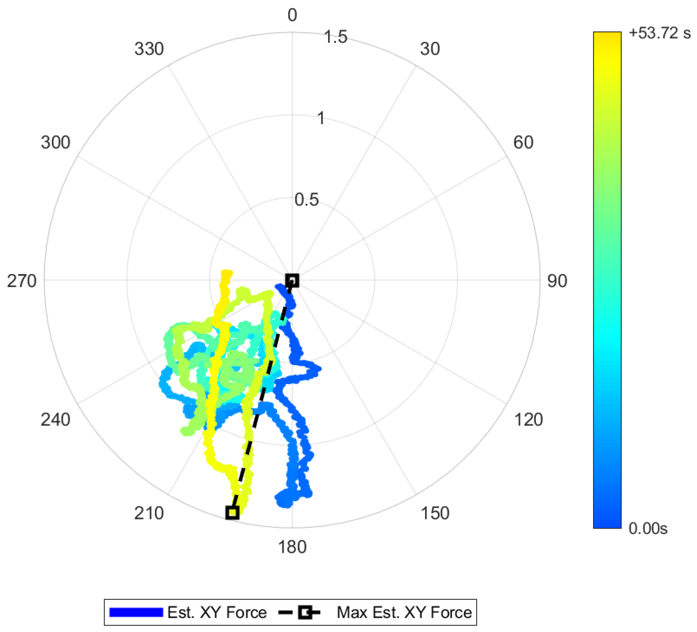
Even though we did not have the real-time information on the actual turbulence profile around the UAV, from the disturbance observer results in
Figure 21i,ii, the magnitude and direction of the airflow could be estimated. As a practical application, the disturbance observer can also be used to estimate the real-time wind direction and magnitude and sketch the wind profile. As an example, in the wind case, the horizontal force applied to the UAV was shown on the polar plot in
Figure 22. Based on the NED coordinate frame, the UAV was located at the origin, with 0 degree corresponding to the +
X and 90 degrees representing the +
Y. The wind generated by the fan was blowing in the
direction. The color bar is associated with the time-series of the experiment, starting from blue and landing at yellow, where the maximum magnitude of the wind and its corresponding direction could be retrieved after the flight. From this polar map, the wind was ≈0.5 N, blowing from the north-east towards the UAV during most of the flight, with the maximum wind occurring at the beginning and at the end.
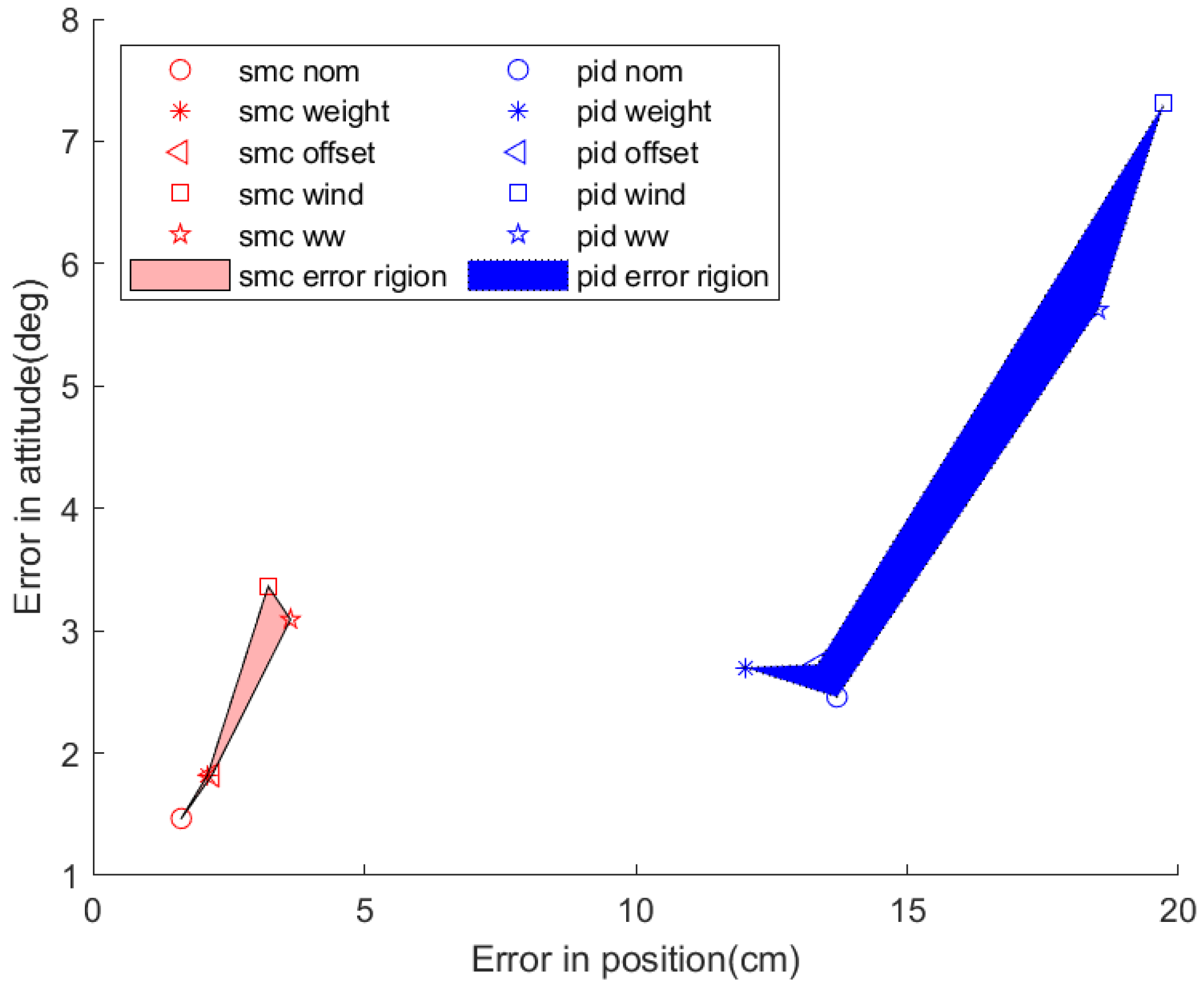
As a short summary of the hover flight experiment, the total error was calculated according to
Table 2 and by
where
denotes the total position error,
denotes the total attitude error,
i and
j represent each degree of freedom, and
x,
y,
z,
r,
p, and
correspond to
X,
Y,
Z,
,
, and
, respectively. The RMS error distribution for a particular controller in each case was scattered and formed a region in
Figure 23, with the horizontal and vertical coordinates indicating the position error and attitude error, respectively. In addition, to distinguish the differences between SMC and PID, their results were displayed in different colors and textures.
In
Figure 23, each marker denotes a different experiment. For example, comparing the SMC with the PID under the nominal condition, the blue circle was farther from the origin than the red circle, which indicated the PID has a larger position and attitude error than the SMC. The colored region enclosed by each experiment has the meaning of deviation under uncertainty, and a smaller area means better adaptation to external disturbances; in other words, the controller adapts faster when uncertainty occurs. When a hanging weight was mounted, the UAV tended to track poorly, with larger position and attitude errors compared to the nominal case, although some exceptions occur; for example, when looking at the PID weight case in
Figure 23 the PID had a smaller attitude error than the SMC. In the presence of the wind, there was no doubt that both SMC and PID had larger tracking errors compared to their own nominal cases. In short, it was clear that SMC showed a better tracking accuracy as well as a better disturbance rejection capacity than the PID controller.
4.3.2. Rectangle
The rectangle trajectory was completed for the nominal, center of mass weight, and offset weight cases. The RMS error from each of these experiments is summarized in
Table 3 for the PID and SMC.
The SMC offered more than a 4× improvement in
X and
Y position tracking. Additionally, the
Z tracking was improved by over 5× with the SMC versus the PID controller. The pitch and roll performance of the SMC was slightly worse than that of the PID. Finally, the yaw error was reduced by a factor of 2. In the yaw error plots, it can be seen that the oscillations for the PID controller are approximately double the amplitude of the SMC yaw oscillations (
Figure 24). This 2 to 1 relationship holds regardless of the applied disturbance. However, when a weight disturbance is added there are some spikes in the PID yaw angle error larger than ±5 degrees, which are not present in the nominal case.
The
position plots in
Figure 24, as well as the captured trajectories from the tracking cameras, show a consistent overshoot in +
X with the PID after the first side of the rectangle is traced. This overshoot was present both with and without added disturbances (see
Figure 25). Interestingly, despite this large and consistent overshoot, the RMS error values in
X and
Y are comparable for the PID controller, suggesting that the overshoot did not single-handedly degrade the
X tracking performance.
The
Z plots show a consistent undershoot in the altitude for the PID, regardless of the applied disturbance. This result is consistent with the 10 cm undershoot seen in the hover-trajectory tracking as well (see
Figure 24 and
Figure 25).
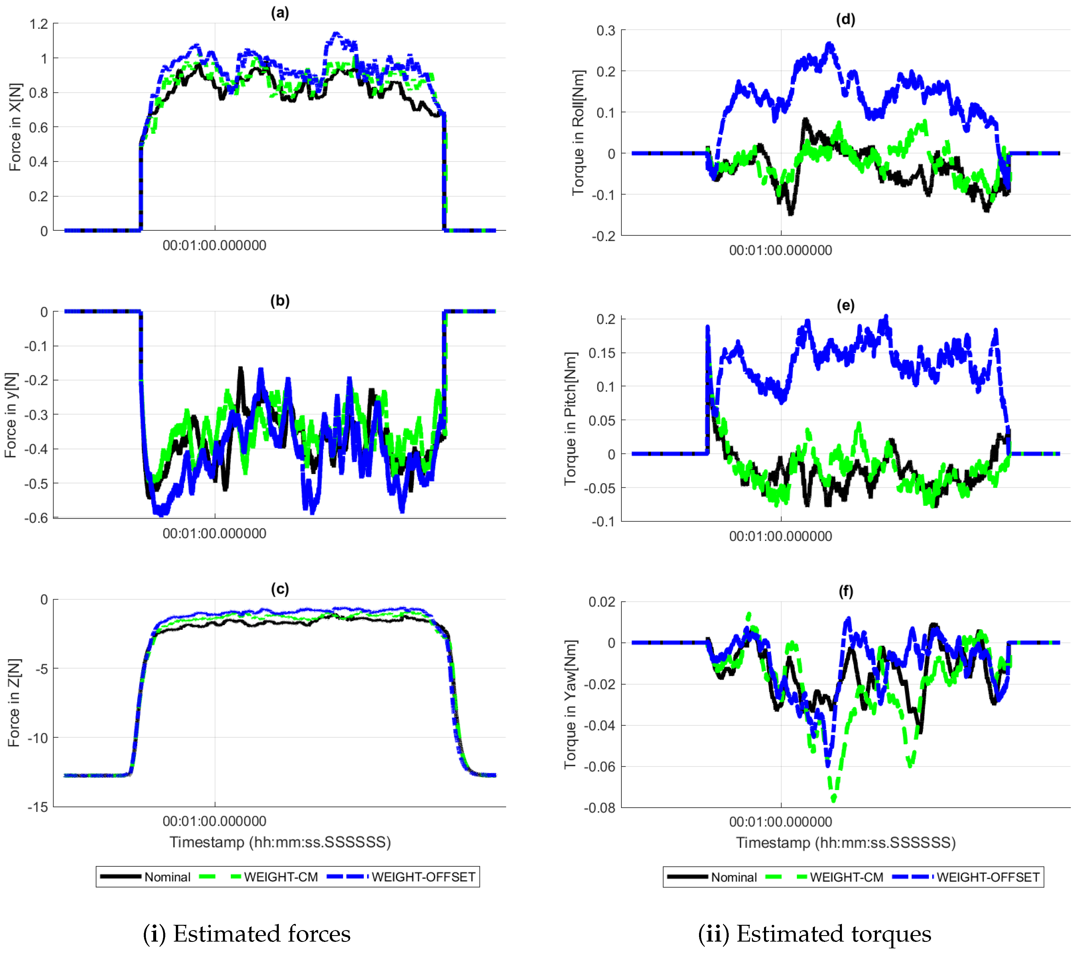
Figure 26i shows the estimated linear forces on the UAV, calculated by the SMC disturbance observer. Unlike the hover case, due to the swinging pendulum motion, there were small disturbance fluctuations with respect to
. However, the
Z disturbances were slightly larger than the nominal case due to the attached weight.
In
Figure 26ii, the estimated torque disturbances are plotted. With the offset weight, constant torque disturbances of ≈0.2 Nm can be seen in pitch and roll. There were minimal differences in yaw disturbance between the test with the center weight and the test with the offset weight; however, their fluctuations became larger compared to the nominal case due to the swinging pendulum.
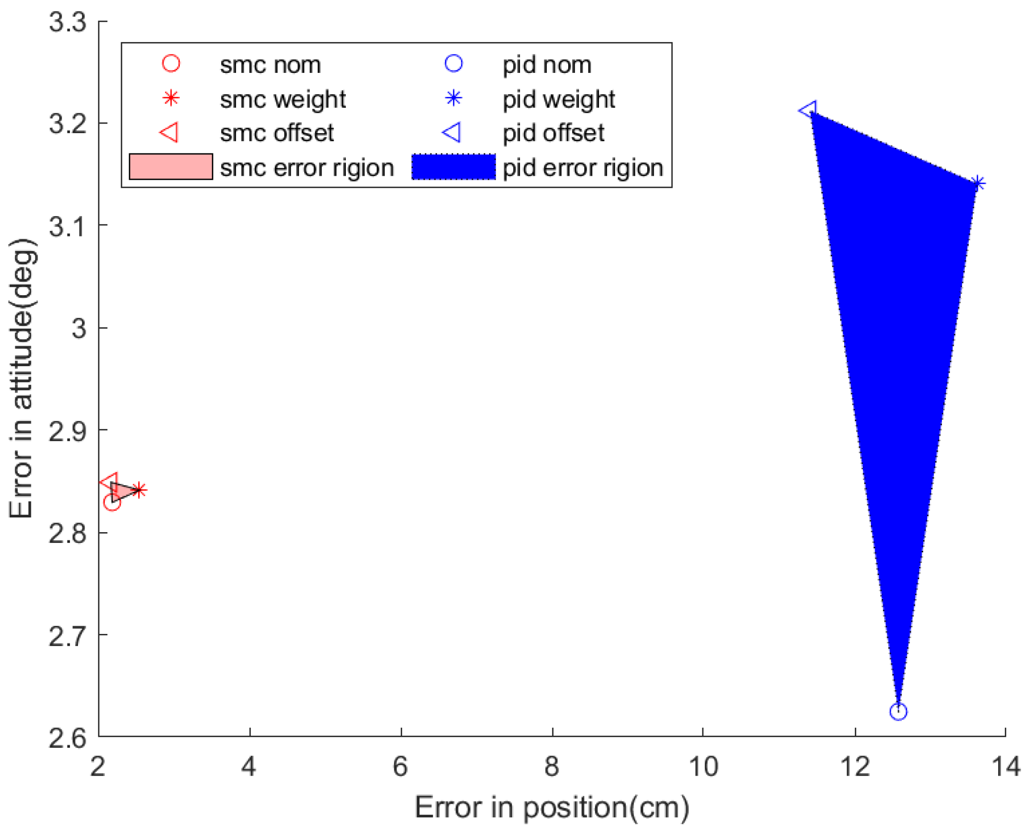
During the rectangular trajectory tracking experiments, the PID has a larger tracking error than the SMC, as shown in
Figure 27. The overall position error reached over 6× of the SMC, and the average attitude error was about the same; however, the deviation of attitude error of PID was much larger than the one of SMC (about 30×). The large blue region enclosed by three standalone experiments implies the behaviors of the PID varying under different uncertainties. Although it had a better angle tracking in the nominal scenario, PID’s performance reduced dramatically in the other disturbance scenarios. Again, from the rectangular experiment results, the SMC overwhelms the PID in both tracking accuracy and disturbance rejection.
4.3.3. Trajectory of a Figure Eight
The figure-eight trajectory was completed for the nominal case and both hanging weight cases. The RMS error from each of these experiments is summarized in
Table 4 for the PID and SMC (
Figure 28).
In the position tracking, the PID had around 1.2–1.5 times the RMS error of that of SMC. The Z tracking was a little more than 2× better with the SMC. In pitch and roll, the SMC error did not change compared to the rectangular trajectory; however, the PID error increased slightly. The difference between the two controllers for pitch and roll tracking was, again, not very significant. In yaw, the SMC outperformed the PID by a small margin with the exception of the offset weight. The PID had around 2× more error in yaw tracking with the offset weight, where the SMC’s performance did not change relative to the other cases.
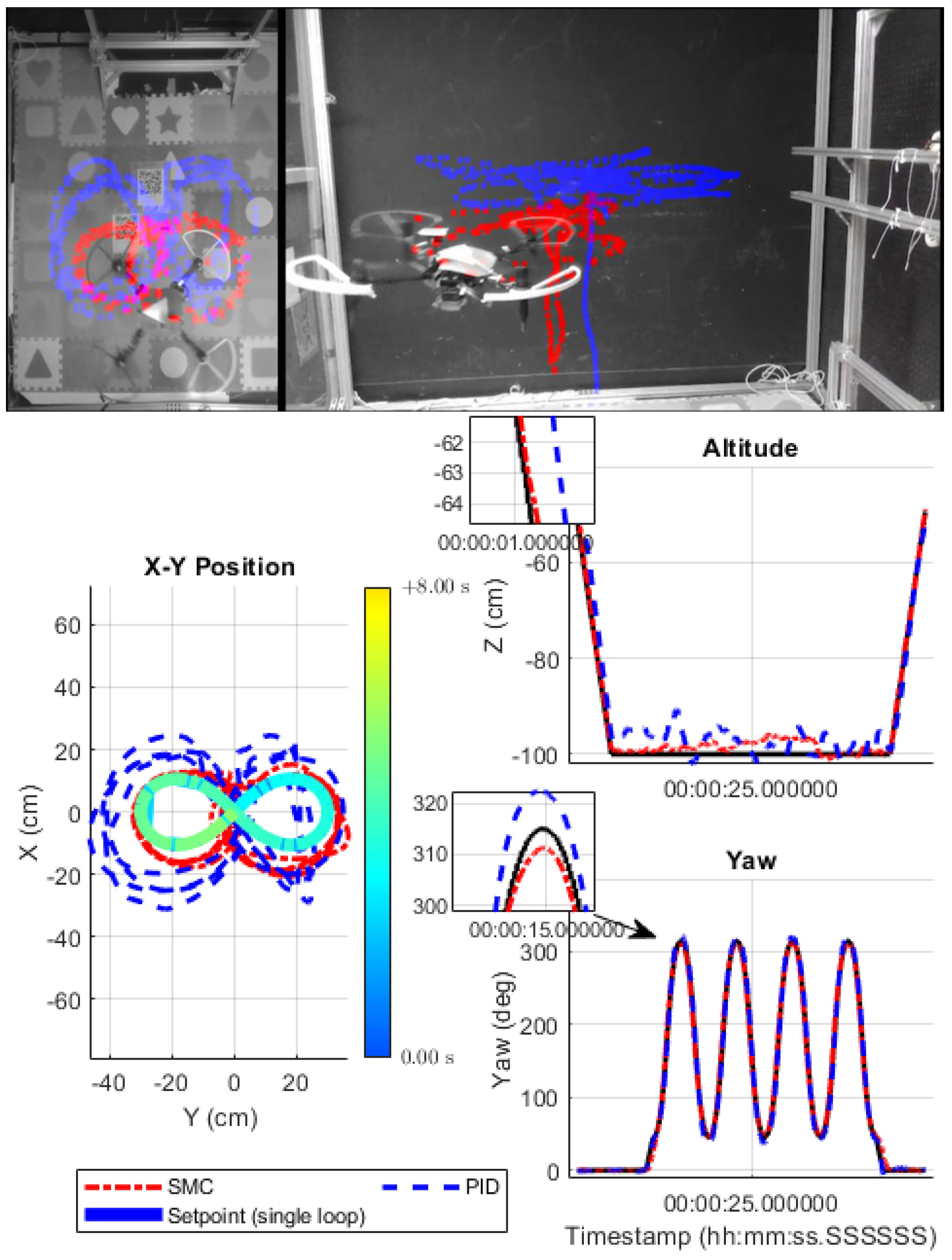
In the
position plots (
Figure 29), the SMC follows a more symmetric path than the PID. The PID has a larger circle on the second half of the trajectory, the left side, than on the first half. This difference is a result of the PID not returning to the origin between the first loop and the second loop. It overshoots the origin on the first loop and is unable to compensate in the second loop.
The Z tracking steady-state offset was not present in the PID controller for the figure-eight trajectory, unlike with the other trajectories, though there was an initial height error after takeoff that was reduced within the first 10 s of the trajectory following. The Z regulation was still poor compared to the SMC. The PID yaw tracking had a slight delay and some overshoot as the direction changed.
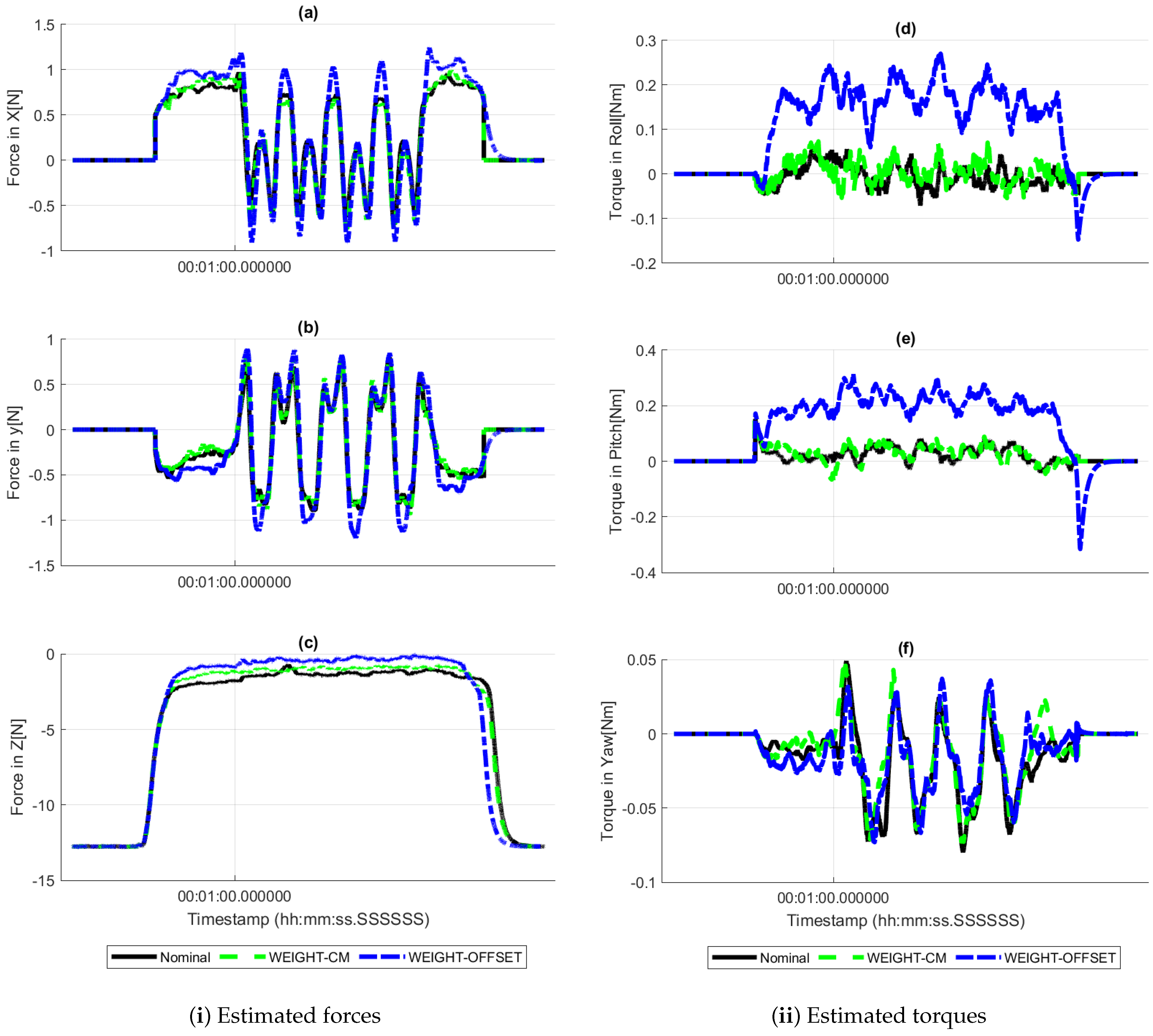
Figure 30i shows the estimated linear force disturbances, from the SMC disturbance observer. The reciprocal oscillations of disturbances in
showed the aerodynamic forces opposing the motion. As the UAV would yaw and turn, the weight would swing out accordingly. Thus, for the offset weight case, due to a larger centrifugal force, the
X and
Y disturbances grew larger, with sharper oscillations; meanwhile,
Z had a larger downward force. Because of the UAV’s aggressive flight motion and rapidly changing attitude, the offset weight could usually swing at an angle of about 30–45 deg.
The pitch and roll disturbances in
Figure 30ii show constant torque offsets of ≈0.2 Nm for the offset weight case, similarly to the rectangle and hover trajectories (
Figure 21ii and
Figure 26ii). The yaw disturbance had oscillations, which were caused by a larger aerodynamic moment as the UAV followed the figure-eight yaw setpoints (
Figure 30ii(f)).
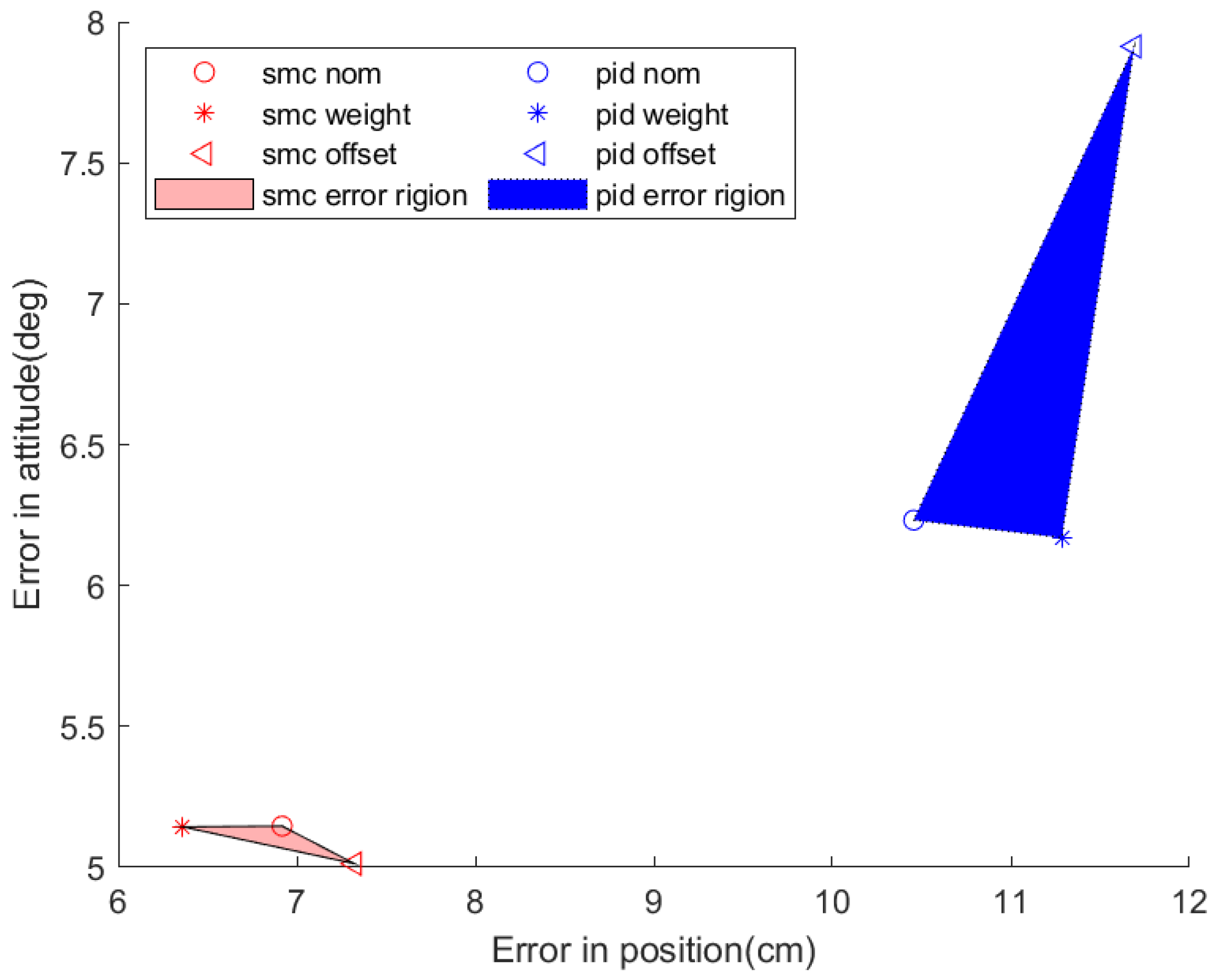
As for the complex figure-eight pattern tracking test, the UAV was commanded to change position and attitude all the time. Both the SMC and the PID have larger position and attitude errors in this case. For the figure-eight nominal case, the PID had 1.5× position error and more than 1.2× attitude error than that of SMC (
Figure 31). For the CM weight case, the PID had 1.8× position error and more than 1.2× attitude error than that of SMC. For the offset weight case, the PID had 1.6× position error and more than 1.5× attitude error than that of SMC. Overall, SMC had a better performance than the PID in this case.


