

Modular Reinforcement Learning for Autonomous UAV Flight Control

Abstract
:1. Introduction
- Six-degrees-of-freedom (6-DOF) environment: For a UAV to perform real-world tasks learned through reinforcement learning, a 6-DOF environment, including the 3D position and orientation, must be considered. However, if the state and action values are both continuous and high-dimensional features, it makes it difficult for a reinforcement learning agent in a 6-DOF environment to learn the features of the environment [9]. Thus, existing reinforcement-learning-based autonomous UAV flight research is limited to conducting experiments after simplifying the action and state spaces in the simulation environment [10,11,12,13,14,15].
- Difficulty in setting the reward: It is difficult to develop reward settings that are suitable for research purposes in the field of reinforcement learning; this difficulty increases as the agent task and environment become increasingly complex. Many researchers have explored reward engineering, which is a process of setting a reward such that the agent can act according to the researcher’s intentions [16]. UAVs need to perform tasks by using not only absolute location information, such as the target coordinates and velocity, but also the relative target point location information. This increases the amount of data that is considered when creating a suitable reward for the task, and the number and type of the location data that are used in each task differ. Therefore, setting a suitable autonomous UAV flight reward is challenging.
- Difficulty performing complex tasks: As a UAV task becomes more difficult, the number of parameters required in the artificial neural network increases. This results in a greater amount of computational resources becoming necessary. Additionally, when performing different tasks sequentially, an artificial neural network receives state and action values with distributions different from those in previous tasks; consequently, model training becomes unstable or the task performance decreases. For this reason, previous autonomous UAV flight research has been limited to performing only a single task [17,18,19,20,21,22]. Thus, research on connecting tasks is necessary for situations in which two tasks must be performed continuously or when complex tasks must be performed.
2. Background
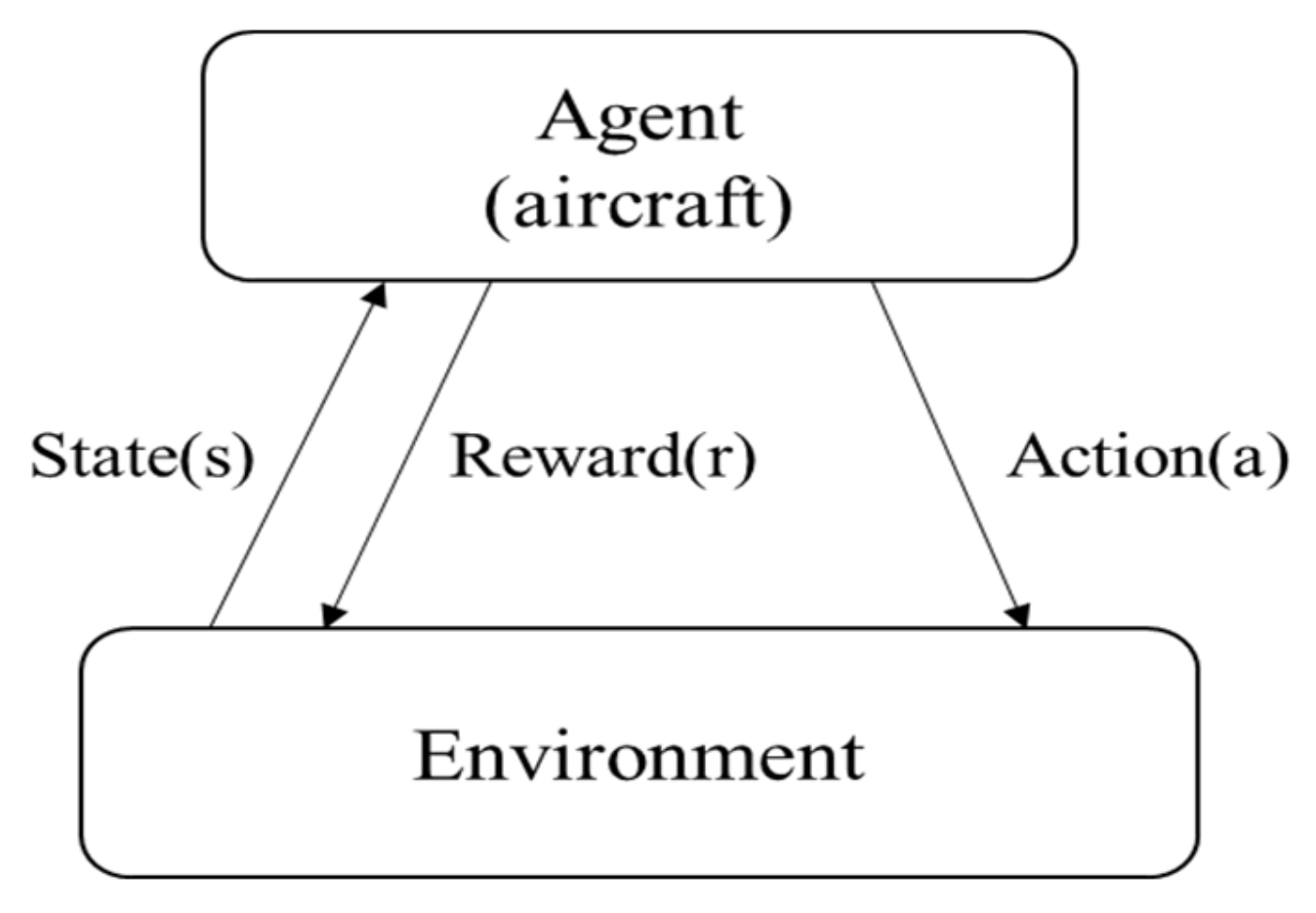
2.1. Reinforcement Learning
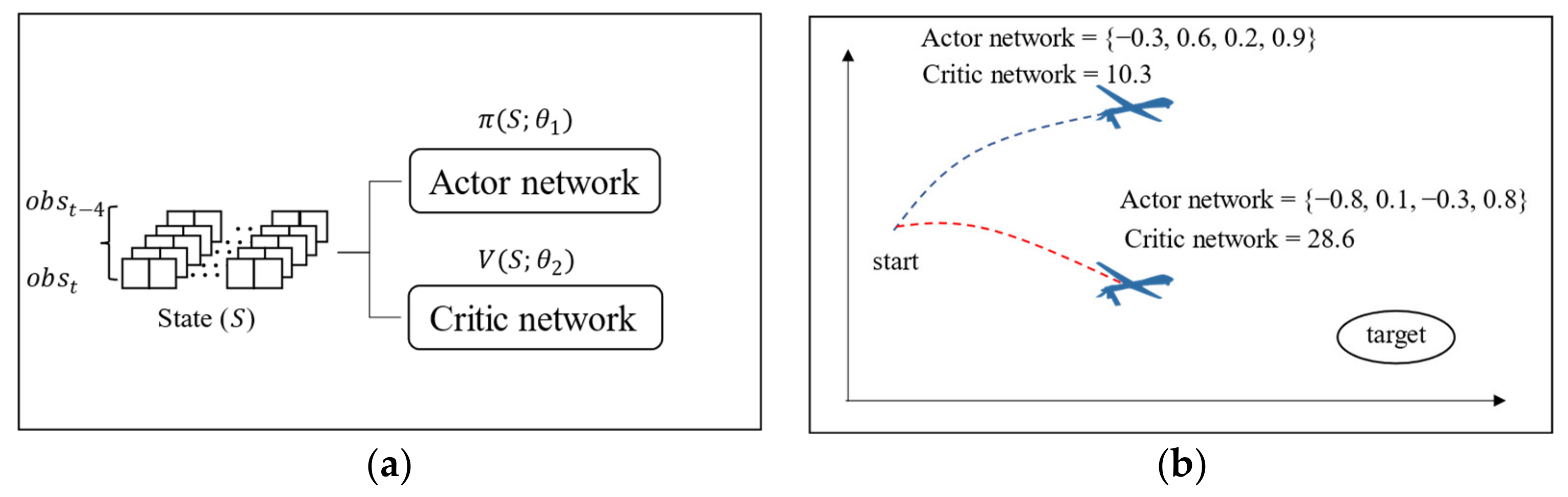
2.2. Actor-Critic Method
2.3. Soft Actor-Critic Algorithm
2.4. Autonomous UAV Maneuvering
3. Proposed Method
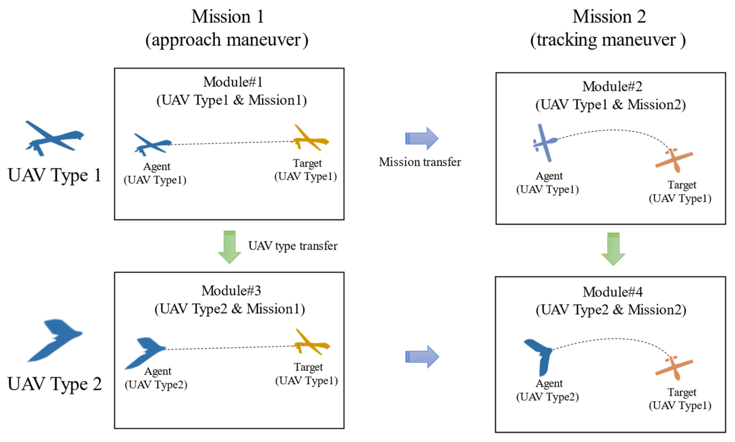
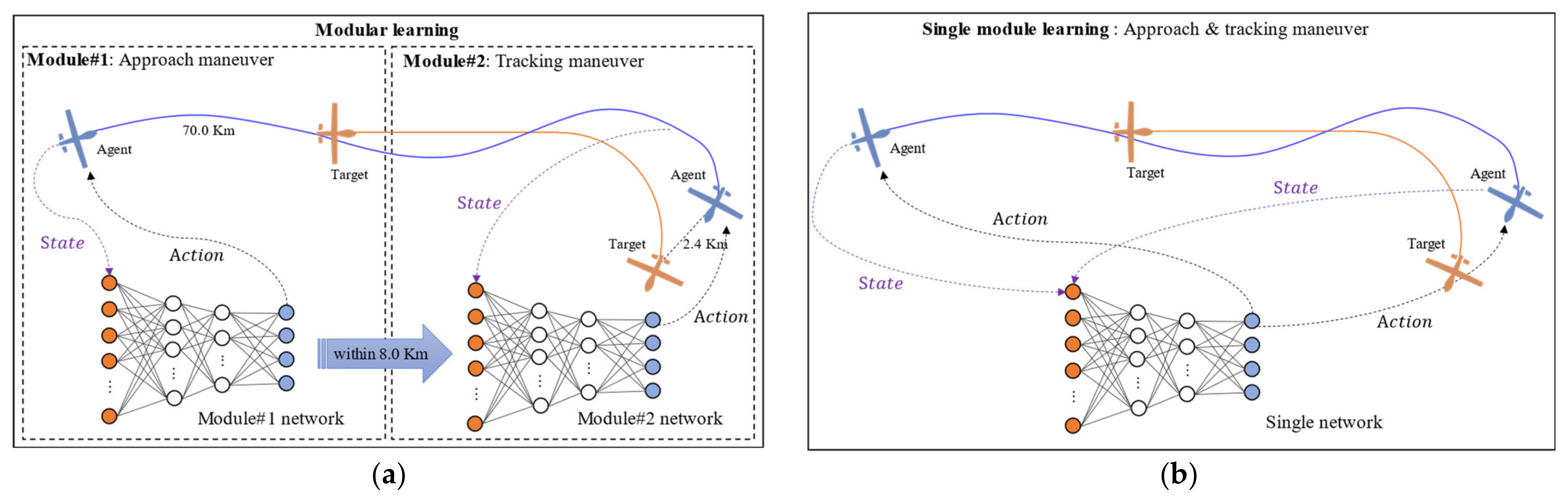
3.1. Modular Learning
3.2. Smooth Module Connection
| Algorithm 1: Soft Actor-Critic and Noise |
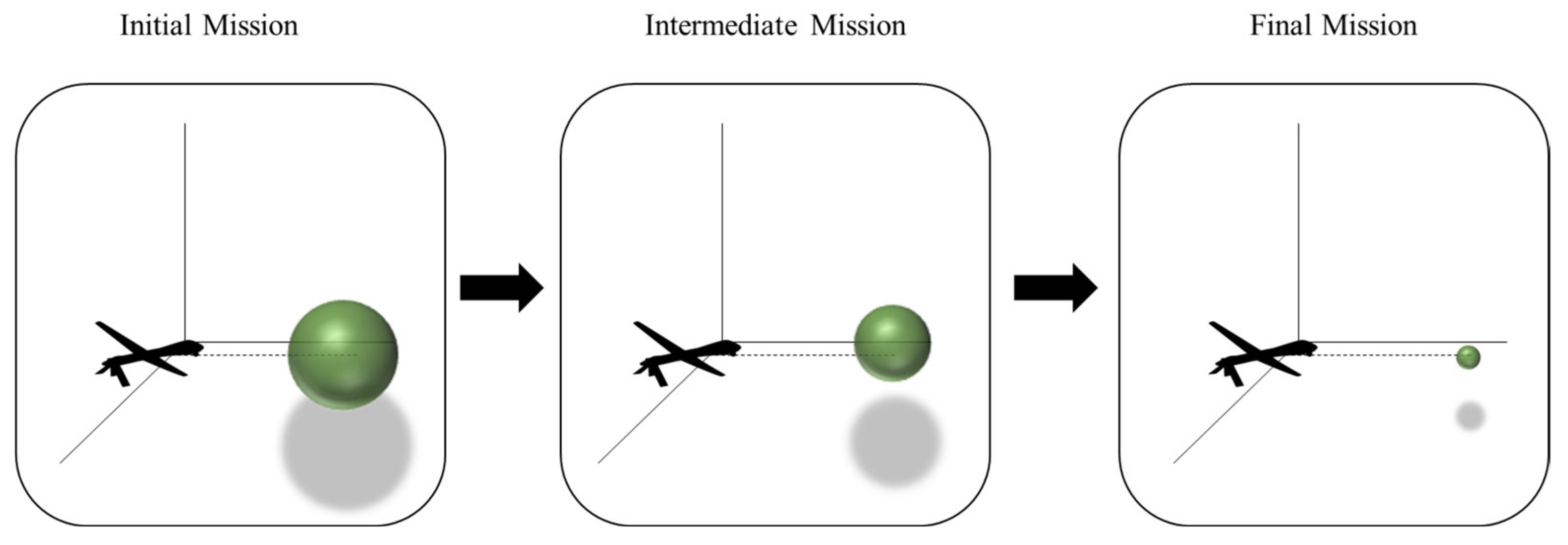
3.3. Curriculum Learning
| Algorithm 2: Soft Actor-Critic and Noise and Curriculum Learning |
4. Experiments
4.1. Simulation Environment Definition
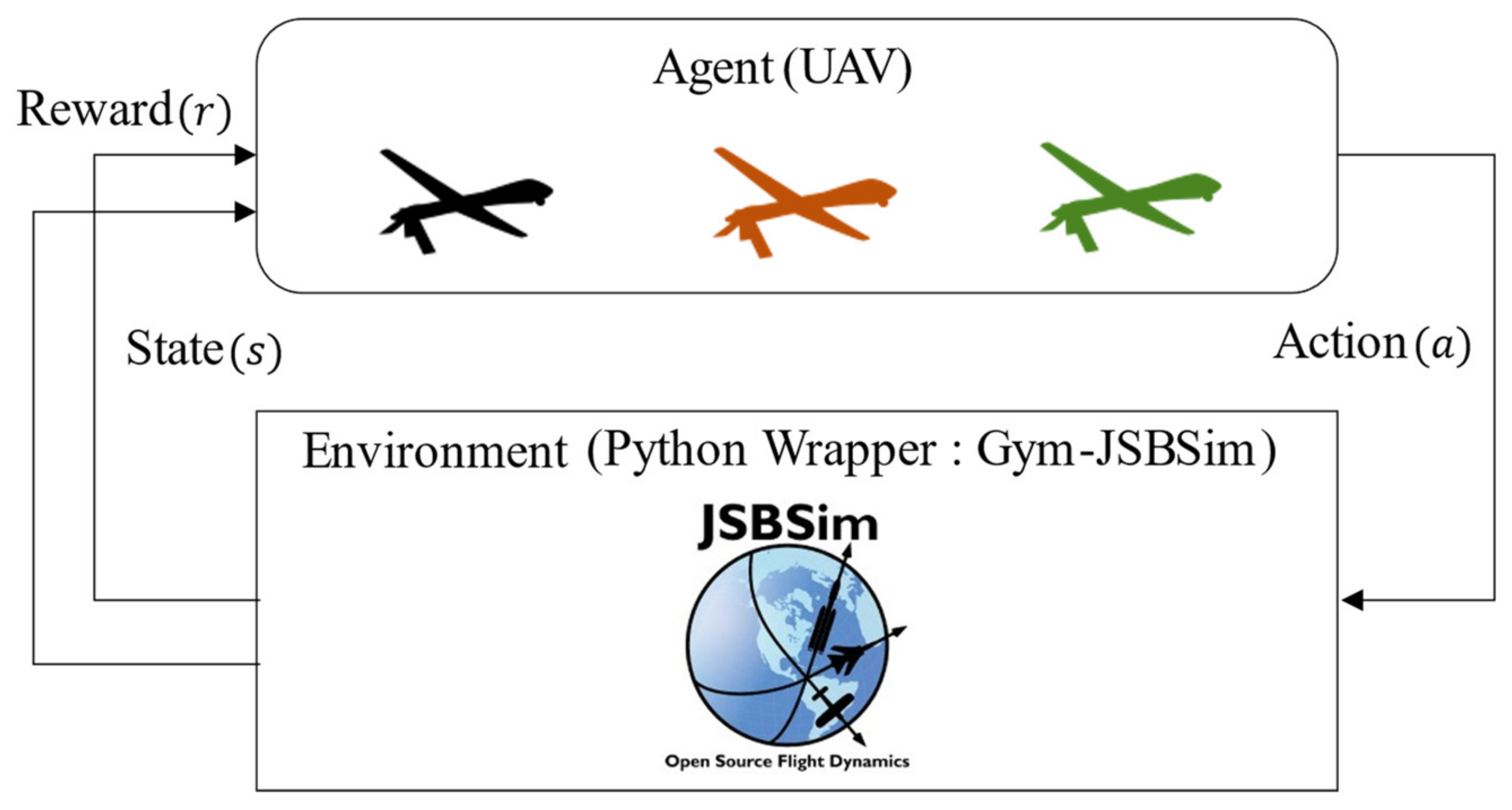
4.1.1. Environment
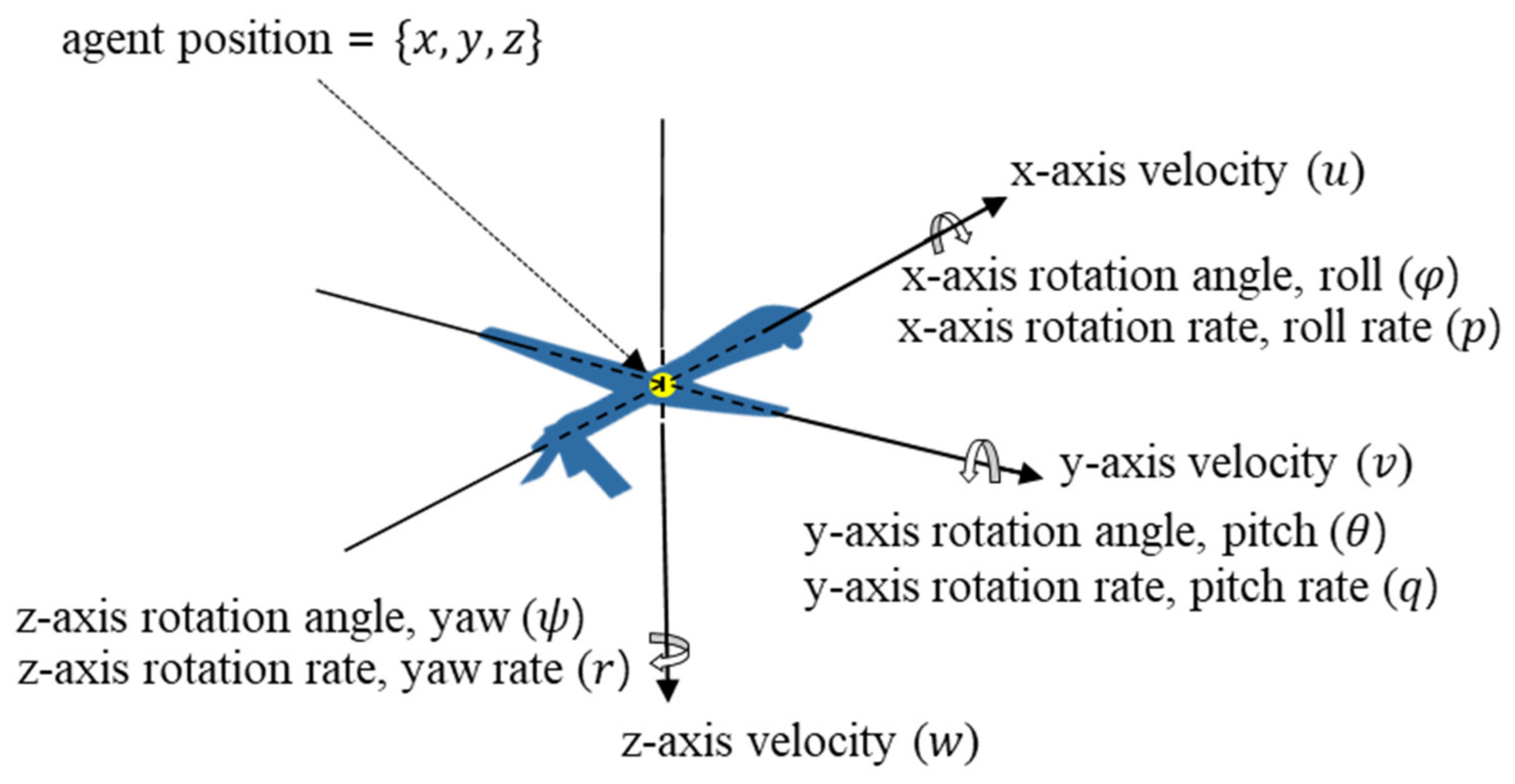
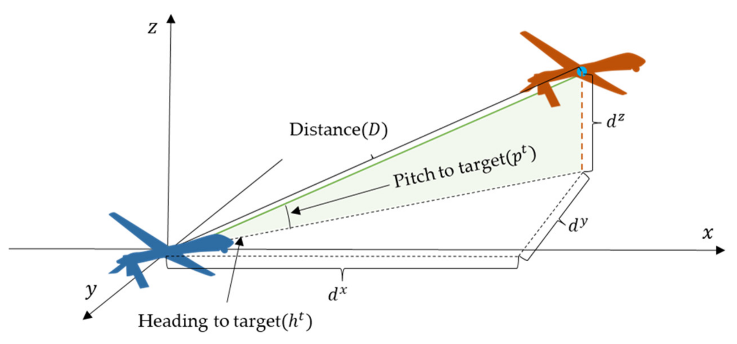
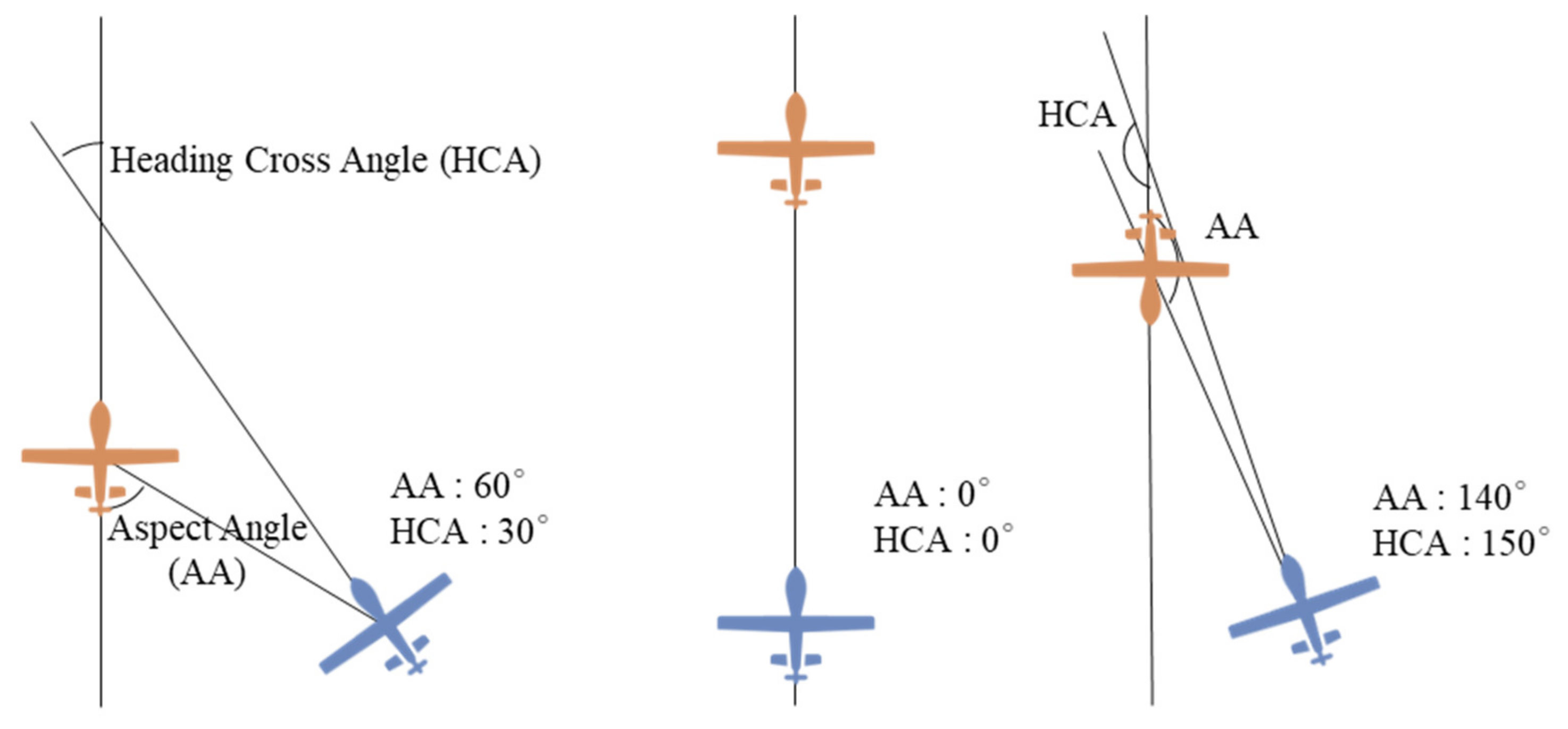
4.1.2. States
4.1.3. Action
4.1.4. Reward
4.2. Experimental Design
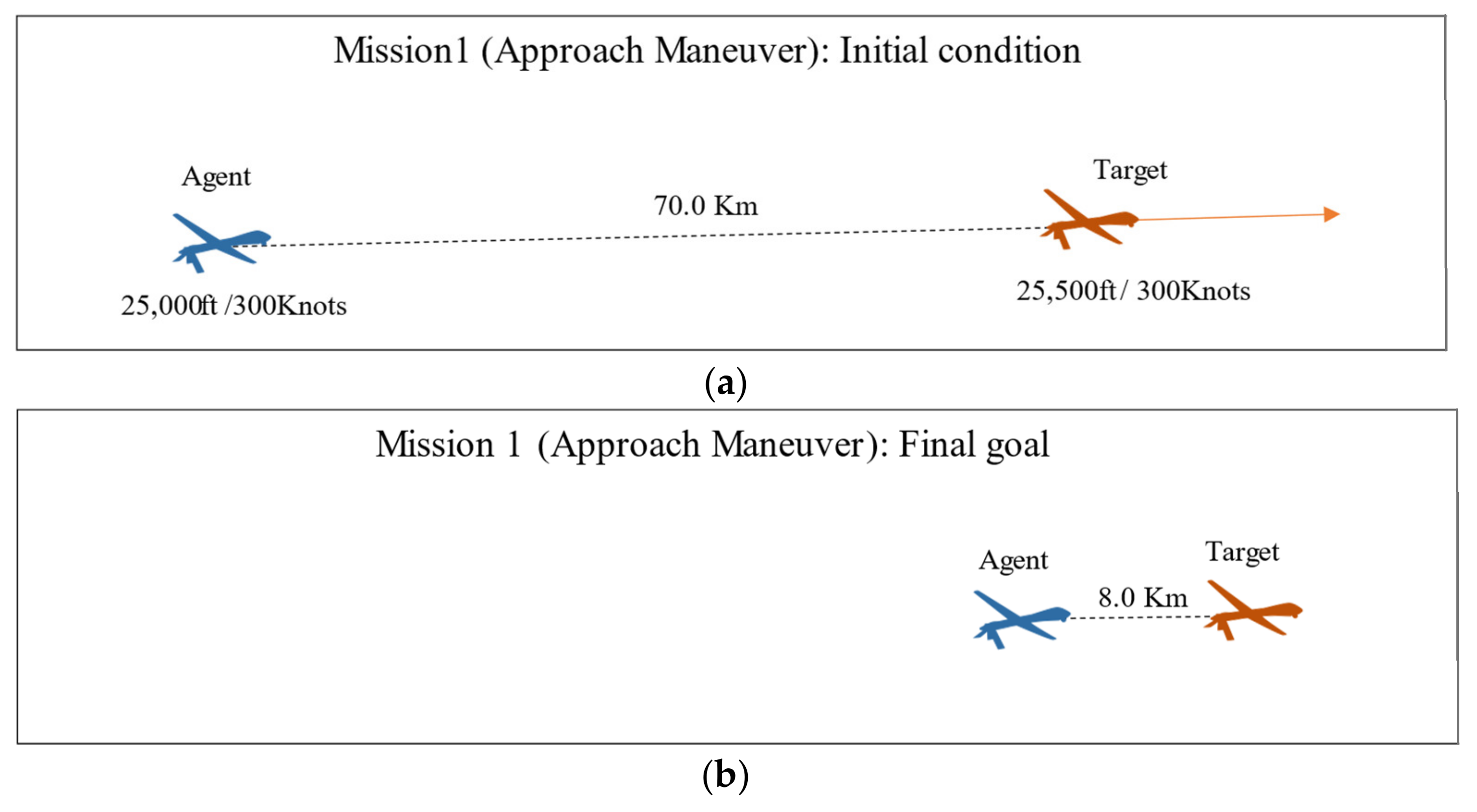
4.2.1. Mission 1 (Approach Maneuver) Definition
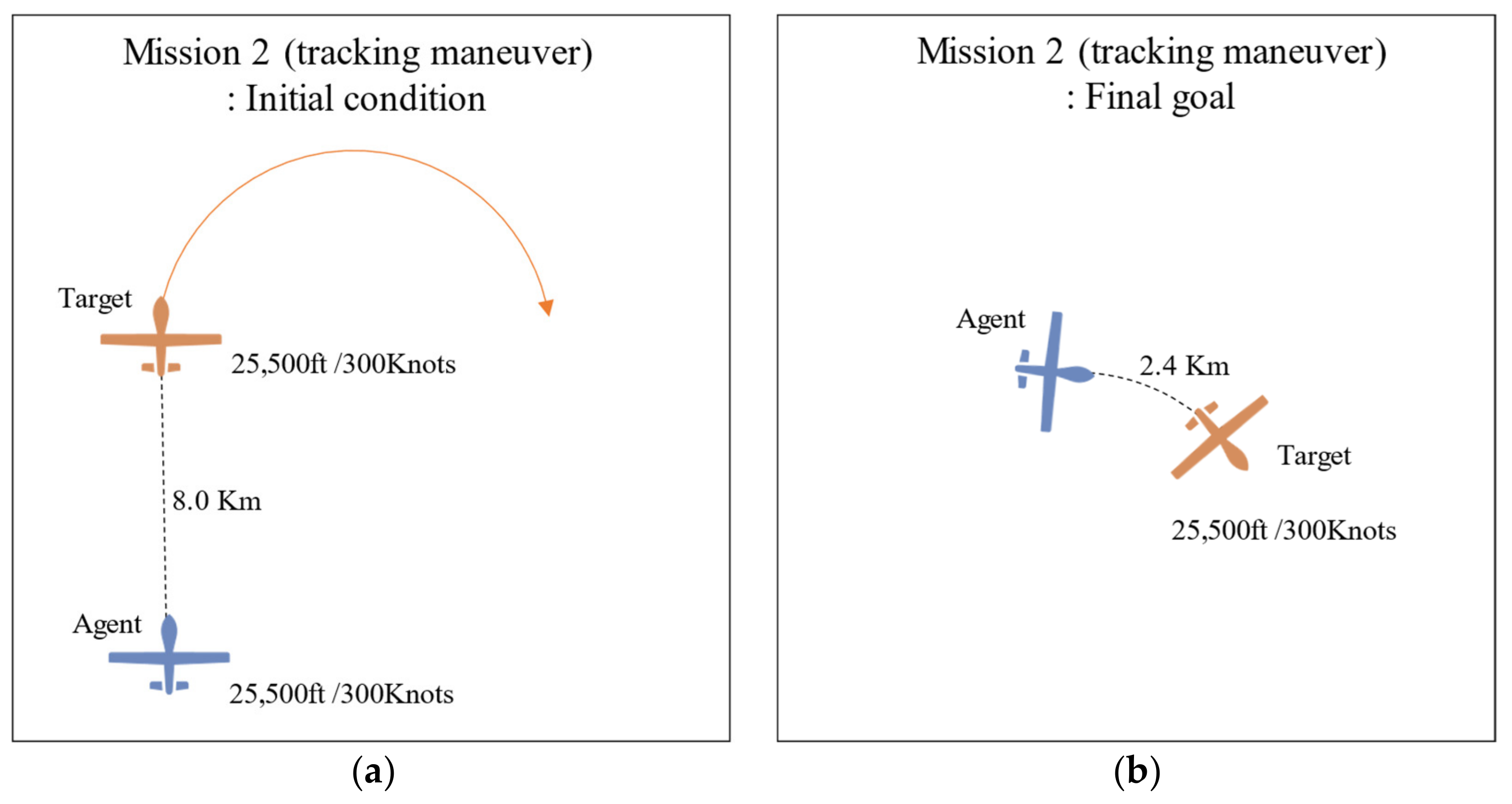
4.2.2. Mission 2 (Tracking Maneuver) Definition
4.2.3. Hyperparameter Settings
4.2.4. Experiment #1: Learning for Each Module
4.2.5. Experiment #2: Transfer Learning Based on the Mission and UAV Type
4.2.6. Experiment #3: Module Connection
4.2.7. Experiment #4: Agent Test
4.3. Experimental Results
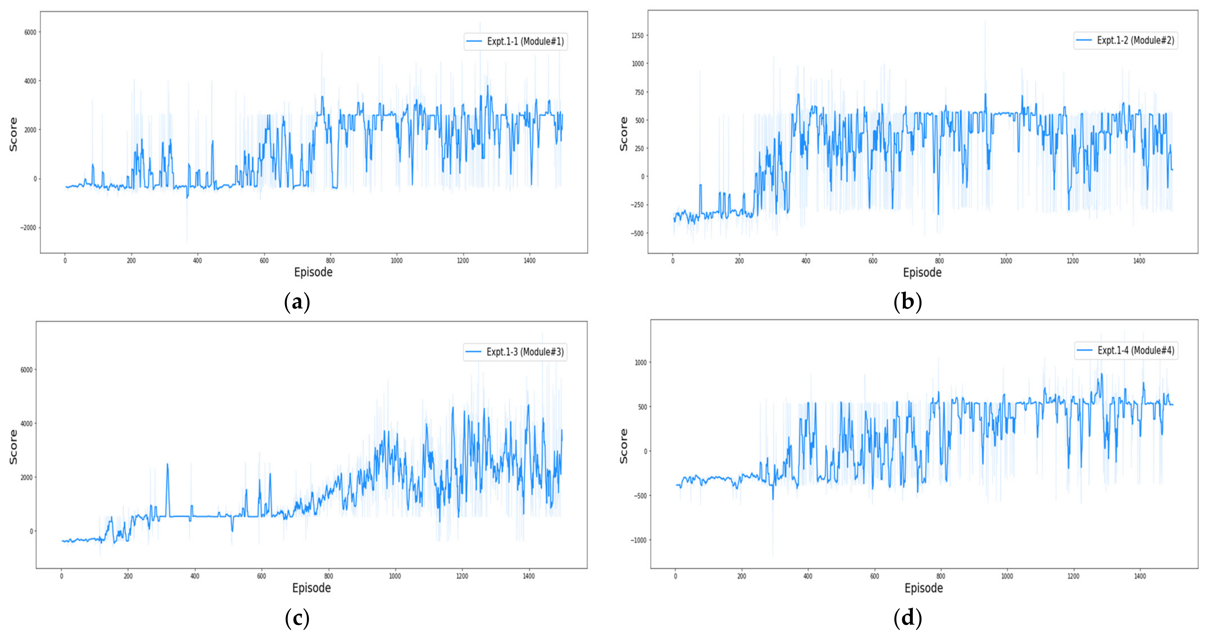
4.3.1. Results of Experiment #1
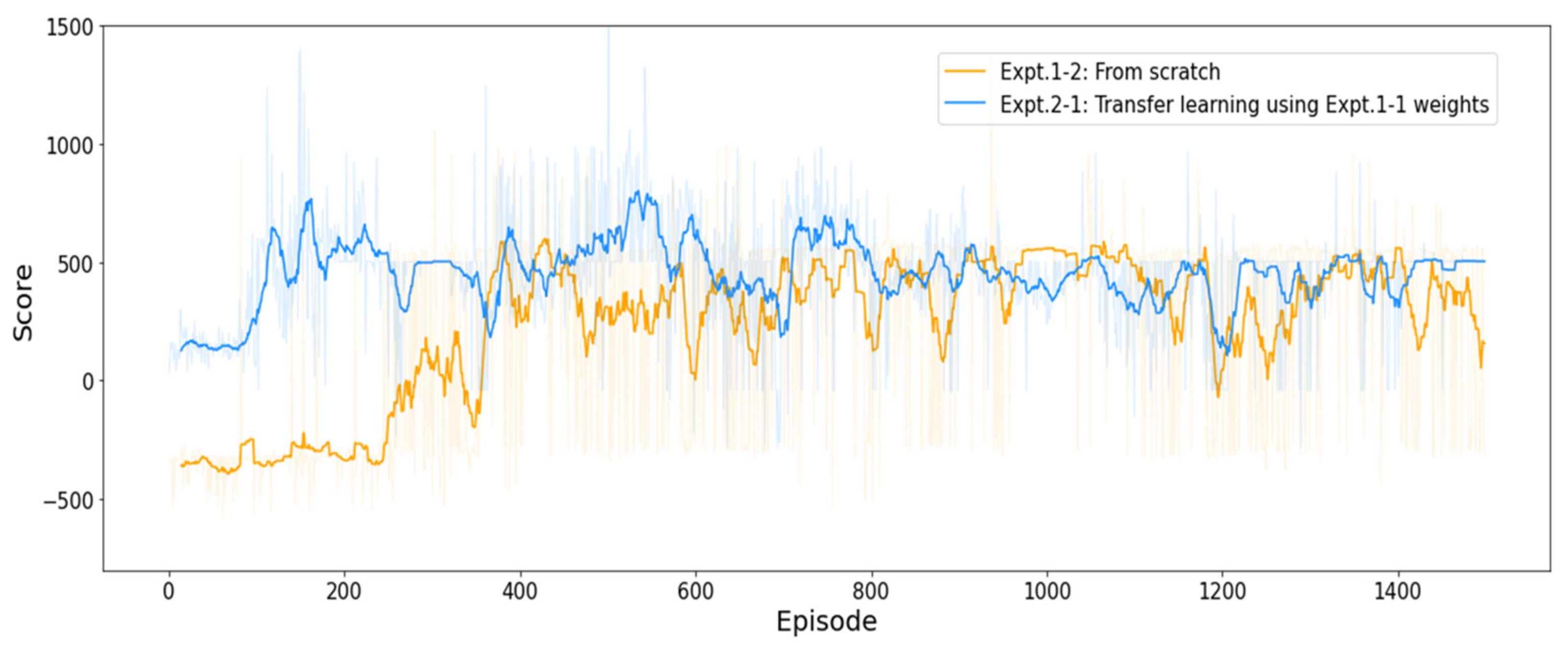
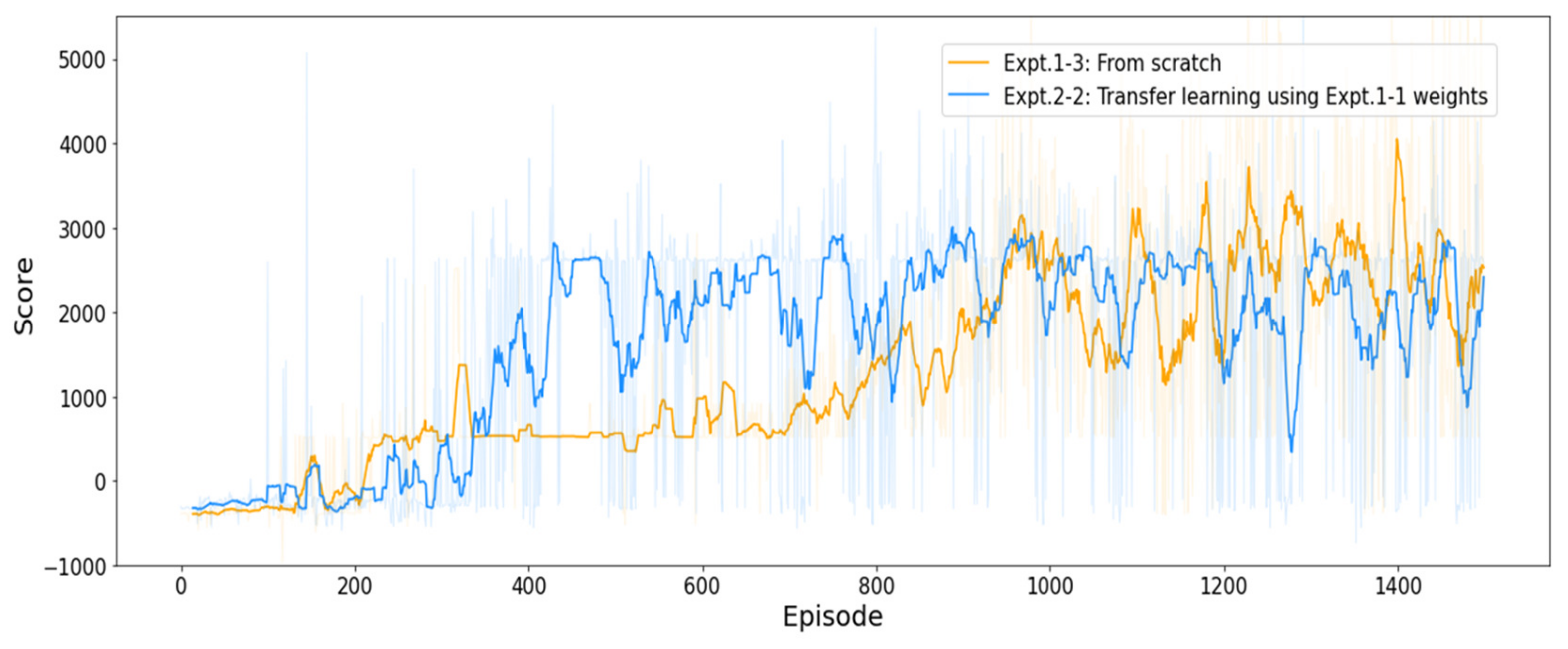
4.3.2. Results of Experiment #2
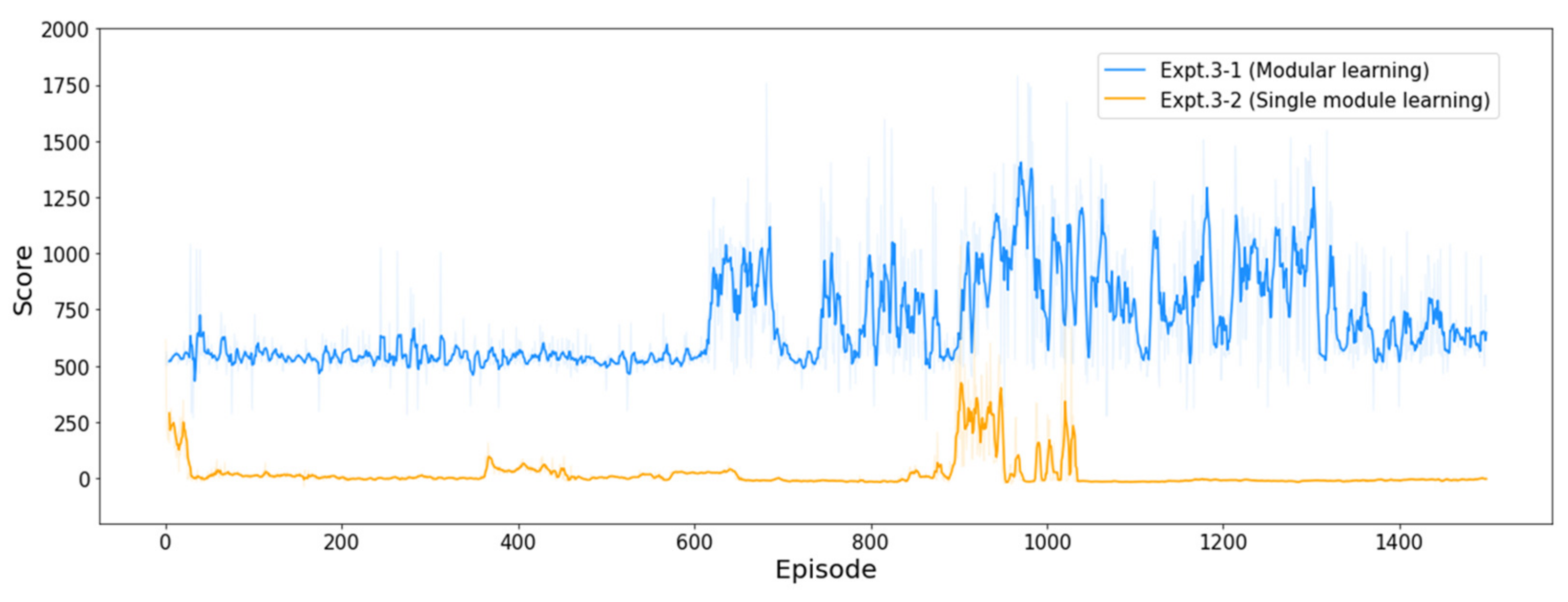
4.3.3. Results of Experiment #3
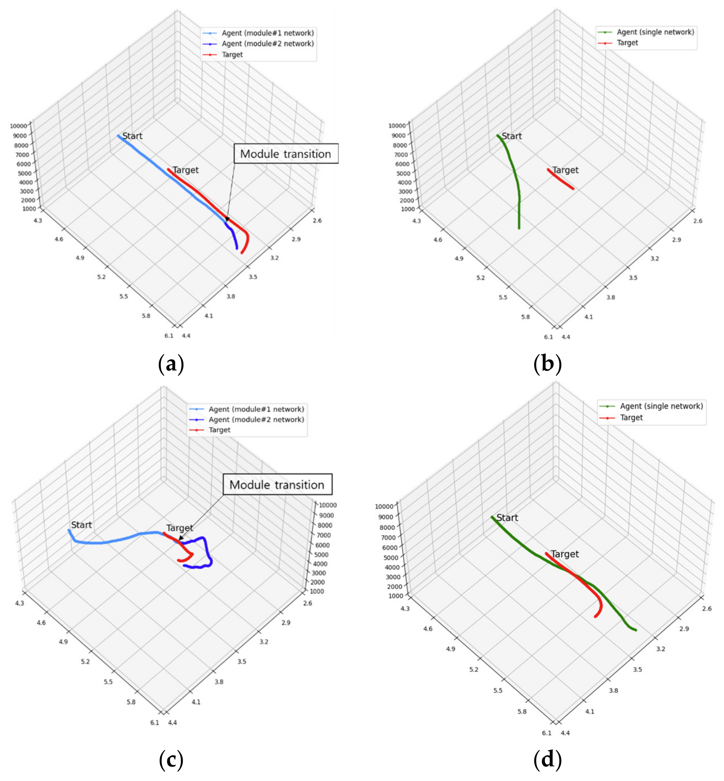
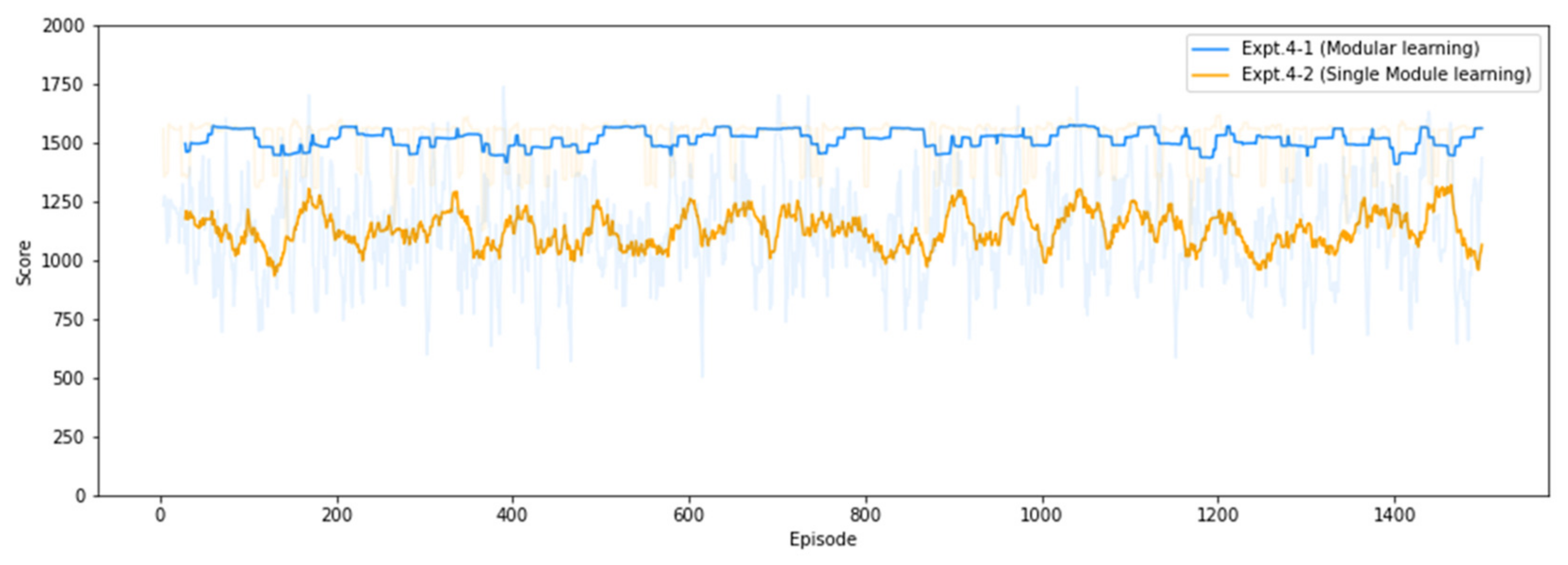
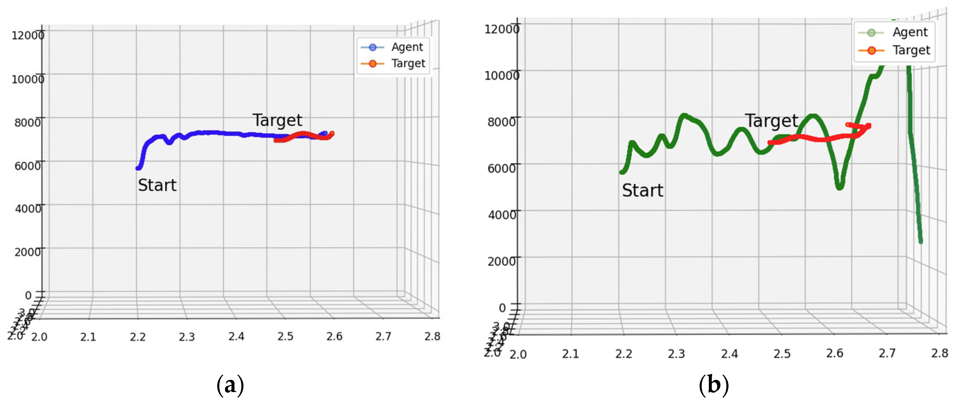
4.3.4. Results of Experiment #4
5. Conclusions
Author Contributions
Funding
Data Availability Statement
Conflicts of Interest
References
- Kim, J.; Kim, S.; Ju, C.; Son, H.I. Unmanned Aerial Vehicles in Agriculture: A Review of Perspective of Platform, Control, and Applications. IEEE Access 2019, 7, 105100–105115. [Google Scholar]
- Eichleay, M.; Evens, E.; Stankevitz, K.; Parker, C. Using the Unmanned Aerial Vehicle Delivery Decision Tool to Consider Transporting Medical Supplies via Drone. Glob. Health Sci. Pract. 2019, 7, 500–506. [Google Scholar] [PubMed] [Green Version]
- Teng, T.H.; Tan, A.H.; Tan, Y.S.; Yeo, A. Self-Organizing Neural Networks for Learning Air Combat Maneuvers. In Proceedings of the International Joint Conference on Neural Networks, Brisbane, Australia, 10–15 June 2012. [Google Scholar]
- Ernest, N.; Carroll, D. Genetic Fuzzy Based Artificial Intelligence for Unmanned Combat Aerial Vehicle Control in Simulated Air Combat Missions. J. Def. Manag. 2016, 6, 1000144. [Google Scholar] [CrossRef]
- NLR-Netherlands Aerospace Centre. Rapid Adaptation of Air Combat Behaviour; Netherlands Aerospace Centre: Amsterdam, The Netherlands, 2016. [Google Scholar]
- Azar, A.T.; Koubaa, A.; Ali Mohamed, N.; Ibrahim, H.A.; Ibrahim, Z.F.; Kazim, M.; Ammar, A.; Benjdira, B.; Khamis, A.M.; Hameed, I.A.; et al. Drone Deep Reinforcement Learning: A Review. Electronics 2021, 10, 999. [Google Scholar]
- Mudrov, M.; Ziuzev, A.; Nesterov, K.; Valtchev, S. Power Electrical Drive Power-Hardware-In-the-Loop System: 2018 X International Conference on Electrical Power Drive Systems (ICEPDS). In Proceedings of the 10th International Conference on Electrical Power Drive Systems (ICEPDS), Novocherkassk, Russia, 3–6 October 2018; ISBN 9781538647134. [Google Scholar]
- Chen, H.; Wang, X.M.; Li, Y. A Survey of Autonomous Control for UAV. In Proceedings of the 2009 International Conference on Artificial Intelligence and Computational Intelligence (AICI), Shanghai, China, 7–8 November 2009; Volume 2, pp. 267–271. [Google Scholar]
- Rocha, T.A.; Anbalagan, S.; Soriano, M.L.; Chaimowicz, L. Algorithms or Actions? A Study in Large-Scale Reinforcement Learning. In Proceedings of the International Joint Conference on Artificial Intelligence (IJCAI-18), Stockholm, Sweden, 13–19 July 2018; pp. 2717–2723. [Google Scholar]
- Yang, Q.; Zhang, J.; Shi, G.; Hu, J.; Wu, Y. Maneuver Decision of UAV in Short-Range Air Combat Based on Deep Reinforcement Learning. IEEE Access 2020, 8, 363–378. [Google Scholar] [CrossRef]
- Wang, Z.; Li, H.; Wu, H.; Wu, Z. Improving Maneuver Strategy in Air Combat by Alternate Freeze Games with a Deep Reinforcement Learning Algorithm. Math. Probl. Eng. 2020, 2020, 7180639. [Google Scholar] [CrossRef]
- Lee, G.T.; Kim, C.O. Autonomous Control of Combat Unmanned Aerial Vehicles to Evade Surface-to-Air Missiles Using Deep Reinforcement Learning. IEEE Access 2020, 8, 226724–226736. [Google Scholar] [CrossRef]
- Yan, C.; Xiang, X.; Wang, C. Fixed-Wing UAVs Flocking in Continuous Spaces: A Deep Reinforcement Learning Approach. Rob. Auton. Syst. 2020, 131, 103594. [Google Scholar] [CrossRef]
- Bohn, E.; Coates, E.M.; Moe, S.; Johansen, T.A. Deep Reinforcement Learning Attitude Control of Fixed-Wing UAVs Using Proximal Policy Optimization. In Proceedings of the 2019 International Conference on Unmanned Aircraft Systems, ICUAS 2019, Atlanta, GA, USA, 11–14 June 2019; Institute of Electrical and Electronics Engineers Inc.: New York, NY, USA, 2019; pp. 523–533. [Google Scholar]
- Tang, C.; Lai, Y.C. Deep Reinforcement Learning Automatic Landing Control of Fixed-Wing Aircraft Using Deep Deterministic Policy Gradient. In Proceedings of the 2020 International Conference on Unmanned Aircraft Systems, ICUAS 2020, Athens, Greece, 1–4 September 2020; Institute of Electrical and Electronics Engineers Inc.: New York, NY, USA, 2020; pp. 1–9. [Google Scholar]
- Dewey, D. Reinforcement Learning and the Reward Engineering Principle. In Proceedings of the Association for the Advancement of Artificial Intelligence, AAAI 2014, Palo Alto, CA, USA, 24–26 March 2014; pp. 13–16. [Google Scholar]
- Koch, W.; Mancuso, R.; West, R.; Bestavros, A. Reinforcement Learning for UAV Attitude Control. ACM Trans. Cyber-Phys. Syst. 2019, 3, 1–21. [Google Scholar] [CrossRef] [Green Version]
- Imanberdiyev, N.; Fu, C.; Kayacan, E.; Chen, I.M. Autonomous Navigation of UAV by Using Real-Time Model-Based Reinforcement Learning. In Proceedings of the 2016 14th International Conference on Control, Automation, Robotics and Vision, ICARCV 2016, Phuket, Thailand, 13–15 November 2016; Institute of Electrical and Electronics Engineers Inc.: New York, NY, USA, 2017. [Google Scholar]
- Liu, C.H.; Chen, Z.; Tang, J.; Xu, J.; Piao, C. Energy-Efficient UAV Control for Effective and Fair Communication Coverage: A Deep Reinforcement Learning Approach. IEEE J. Sel. Areas Commun. 2018, 36, 2059–2070. [Google Scholar] [CrossRef]
- Liu, P.; Ma, Y. A Deep Reinforcement Learning Based Intelligent Decision Method for UCAV Air Combat. In Communications in Computer and Information Science; Springer: Berlin/Heidelberg, Germany, 2017; Volume 751, pp. 274–286. [Google Scholar]
- Zhang, H.; Huang, C. Maneuver Decision-Making of Deep Learning for UCAV Thorough Azimuth Angles. IEEE Access 2020, 8, 12976–12987. [Google Scholar] [CrossRef]
- Pham, H.X.; La, H.M.; Feil-Seifer, D.; Van Nguyen, L. Reinforcement Learning for Autonomous UAV Navigation Using Function Approximation. In Proceedings of the 2018 IEEE International Symposium on Safety, Security, and Rescue Robotics, SSRR, Philadelphia, PA, USA, 6–8 August 2018; Institute of Electrical and Electronics Engineers Inc.: New York, NY, USA, 2018. [Google Scholar]
- Berndt, J.S. JSBSim: An Open Source Flight Dynamics Model in C++. In Proceedings of the AIAA Modeling and Simulation Technologies Conference and Exhibit, Providence, RI, USA, 16–19 August 2004. [Google Scholar]
- Pack Kaelbling, L.; Littman, M.L.; Moore, A.W.; Hall, S. Reinforcement Learning: A Survey. J. Artiicial Intell. Res. 1996, 4, 237–285. [Google Scholar]
- Bhatnagar, S.; Sutton, R.S.; Ghavamzadeh, M.; Lee, M. Natural Actor-Critic Algorithms. Automatica 2009, 45, 2471–2482. [Google Scholar] [CrossRef] [Green Version]
- Haarnoja, T.; Zhou, A.; Abbeel, P.; Levine, S. Soft Actor-Critic: Off-Policy Maximum Entropy Deep Reinforcement Learning with a Stochastic Actor. In Proceedings of the 35th International Conference on Machine Learning (PMLR), Stockholm, Sweden, 10–15 July 2018; pp. 1861–1870. [Google Scholar]
- Transfer, M.; Devin, C.; Darrell, T.; Abbeel, P. Learning modular neural network policies for multi-task and multi-robot transfer. In Proceedings of the 2017 IEEE International Conference on Robotics and Automation (ICRA), Singapore, 29 May–3 June 2017. [Google Scholar]
- Zhu, Z.; Lin, K.; Zhou, J. Transfer Learning in Deep Reinforcement Learning: A Survey. arXiv 2020, arXiv:2009.07888. [Google Scholar]
- Bengio, Y.; Louradour, J.; Collobert, R.; Weston, J. Curriculum Learning. In Proceedings of the 26th Annual International Conference on Machine Learning, Montreal, QC, Canada, 14–18 June 2009; pp. 41–48. [Google Scholar]
- Narvekar, S.; Peng, B.; Leonetti, M.; Sinapov, J.; Taylor, M.E.; Stone, P. Curriculum Learning for Reinforcement Learning Domains: A Framework and Survey. J. Mach. Learn. Res. 2020, 21, 7382–7431. [Google Scholar]
- Sutton, R.S.; Barto, A.G. Reinforcement Learning: An Introduction, 2nd ed.; The MIT Press: Cambridge, MA, USA, 2015. [Google Scholar]
- Cereceda, O. A Simplified Manual of the JSBSim Open-Source Software FDM for Fixed-Wing UAV Applications. Memorial University. 2019. Available online: https://research.library.mun.ca/13798/1/Tech_Report_JSBSim.pdf (accessed on 5 June 2023).
- Pope, A.P.; Ide, J.S.; Micovic, D.; Diaz, H.; Rosenbluth, D.; Ritholtz, L.; Twedt, J.C.; Walker, T.T.; Alcedo, K.; Javorsek, D. Hierarchical Reinforcement Learning for Air-to-Air Combat. In Proceedings of the 2021 International Conference on Unmanned Aircraft Systems (ICUAS), Athens, Greece, 15–18 June 2021; Institute of Electrical and Electronics Engineers Inc.: New York, NY, USA, 2021; pp. 275–284. [Google Scholar]
- Rennie, G. Autonomous Control of Simulated Fixed Wing Aircraft Using Deep Reinforcement Learning. Master’s Thesis, The University of Bath, Bath, UK, 2018. [Google Scholar]
- Wiering, M.A.; Van Otterlo, M. Reinforcement Learning: State-of-the-Art; Springer: Berlin/Heidelberg, Germany, 2012; ISBN 9783642015267. [Google Scholar]


| State | Definition | State | Definition |
|---|---|---|---|
| x-axis position | y-axis position | ||
| z-axis position | x-axis velocity | ||
| y-axis velocity | z-axis velocity | ||
| x-axis rotation angle (roll) | y-axis rotation angle (pitch) | ||
| z-axis rotation angle (yaw) | x-axis rotation rate (roll rate) | ||
| y-axis rotation rate (pitch rate) | z-axis rotation rate (yaw rate) |
| State | Definition | State | Definition |
|---|---|---|---|
| x-axis distance between the UAV and target | y-axis distance between the UAV and target | ||
| z-axis distance between the UAV and target | Pitch angle to target | ||
| Heading angle to target | Distance to target | ||
| Aspect angle | Heading cross-angle |
| Action | Definition | Action | Definition |
|---|---|---|---|
| X-axis stick position (−1 to 1) | Throttle angle (0 to 1) | ||
| Y-axis stick position (−1 to 1) | Rudder pedal angle (−1 to 1) |
| Mission 1 (approach maneuver) | 2500 | 15.0 km | 0.02 | 8.0 km | ||
| Mission 2 (tracking maneuver) | 500 | 4.6 km | 0.02 | 2.4 km |
| Description | |
|---|---|
| Expt. 1-1 | Train Module #1 (UAV Type 1 & Mission 1) from scratch |
| Expt. 1-2 | Train Module #2 (UAV Type 1 & Mission 2) from scratch |
| Expt. 1-3 | Train Module #3 (UAV Type 2 & Mission 1) from scratch |
| Expt. 1-4 | Train Module #4 (UAV Type 2 & Mission 2) from scratch |
| Description | |
|---|---|
| Expt. 2-1 | Transfer learning by applying the weights from Experiment 1-1 to Module #2 |
| Expt. 2-2 | Transfer learning by applying the weights from Experiment 1-1 to Module #3 |
| Description | |
|---|---|
| Expt. 3-1 | Connecting the approach maneuver and tracking maneuver learned in each network |
| Expt. 3-2 | Learning the approach maneuver and tracking maneuver with a single network |
| Description | |
|---|---|
| Expt. 4-1 | Testing the agent trained with modular learning in Experiment 3-1 |
| Expt. 4-2 | Testing the agent trained with a single network in Experiment 3-2 |
| Min Score | Max Score | Mean Score | Cumulative Successes | |
|---|---|---|---|---|
| Expt. 1-1: Module #1 (UAV Type 1 & Mission 1) | −2595.25 | 6383.08 | 1127.48 | 684 |
| Expt. 1-2: Module #2 (UAV Type 1 & Mission 2) | −583.51 | 1371.83 | 233.15 | 908 |
| Expt. 1-3: Module #3 (UAV Type 2 & Mission 1) | −975.43 | 7364.83 | 1285.82 | 304 |
| Expt. 1-4: Module #4 (UAV Type 2 & Mission 2) | −1194.26 | 1349.59 | 143.26 | 797 |
| Min Score | Max Score | Mean Score | Cumulative Successes | |
|---|---|---|---|---|
| Expt. 2-1 (transfer learning) | −283.89 | 1620.16 | 452.16 | 957 |
| Expt. 1-2 (from scratch) | −583.51 | 1371.83 | 233.15 | 908 |
| Min Score | Max Score | Mean Score | Cumulative Successes | |
|---|---|---|---|---|
| Expt. 2-2 (transfer learning) | −738.35 | 5772.40 | 1622.16 | 855 |
| Expt. 1-3 (from scratch) | −975.43 | 7364.83 | 1285.82 | 304 |
| Min Score | Max Score | Mean Score | Cumulative Successes | |
|---|---|---|---|---|
| Expt. 3-1 (modular learning) | 258.95 | 1788.80 | 685.07 | 1357 |
| Expt. 3-2 (single network learning) | −37.51 | 1034.33 | 18.16 | 11 |
| Min Score | Max Score | Mean Score | Cumulative Successes | |
|---|---|---|---|---|
| Expt. 4-1 (modular learning) | 42.39 | 1882.44 | 1514.98 | 1435 |
| Expt. 4-2 (single network learning) | −42.56 | 1845.80 | 1130.81 | 696 |
Disclaimer/Publisher’s Note: The statements, opinions and data contained in all publications are solely those of the individual author(s) and contributor(s) and not of MDPI and/or the editor(s). MDPI and/or the editor(s) disclaim responsibility for any injury to people or property resulting from any ideas, methods, instructions or products referred to in the content. |
© 2023 by the authors. Licensee MDPI, Basel, Switzerland. This article is an open access article distributed under the terms and conditions of the Creative Commons Attribution (CC BY) license (https://creativecommons.org/licenses/by/4.0/).
Share and Cite
Choi, J.; Kim, H.M.; Hwang, H.J.; Kim, Y.-D.; Kim, C.O. Modular Reinforcement Learning for Autonomous UAV Flight Control. Drones 2023, 7, 418. https://doi.org/10.3390/drones7070418
Choi J, Kim HM, Hwang HJ, Kim Y-D, Kim CO. Modular Reinforcement Learning for Autonomous UAV Flight Control. Drones. 2023; 7(7):418. https://doi.org/10.3390/drones7070418
Chicago/Turabian StyleChoi, Jongkwan, Hyeon Min Kim, Ha Jun Hwang, Yong-Duk Kim, and Chang Ouk Kim. 2023. "Modular Reinforcement Learning for Autonomous UAV Flight Control" Drones 7, no. 7: 418. https://doi.org/10.3390/drones7070418