Distributed Dynamic Surface Control for a Class of Quadrotor UAVs with Input Saturation and External Disturbance

Abstract

An adaptive dynamic surface trajectory tracking control method based on the Nussbaum function is proposed for a class of quadrotor UAVs encountering unknown external disturbances and unidentified nonlinearities. By transforming controller expressions into numerical solutions, the challenge of overly complex controller design expressions is addressed, simplifying the overall controller design process and enhancing the efficiency of simulation programs. Additionally, an adaptive controller based on Nussbaum gain is introduced to effectively resolve actuator saturation issues. This approach mitigates complexities associated with traditional control design and ensures smooth operation of the quadrotor UAVs. The proposed methodology offers promising prospects for enhancing the robustness and performance of quadrotor UAVs under uncertain operating conditions. Finally, to validate the effectiveness of the proposed control scheme, a hardware-in-the-loop experimental setup is constructed. The dynamic model of the quadrotor UAVs and the proposed controller scheme are implemented on the Rapid Control Prototype (RCP) and Real-Time Simulator (RTS), respectively. This facilitates a semi-physical simulation experiment, providing a basis for the subsequent application of the control scheme to actual aerial vehicles. The concluding experimental results affirm the effectiveness of the proposed control scheme and highlight its potential for practical applications.

1. Introduction

In recent years, drones have garnered increasing attention, with their applications expanding significantly across both civilian and military domains. In the civilian sector, they are frequently employed for tourism photography [1], formation flight performances [2,3], air quality monitoring [4], forest fire surveillance [5], remote sensing imagery for precision agriculture [6], and other civilian applications. In the military realm, drones serve as military relay networks [7] and are also utilized in swarming combat systems [8]. The role of UAVs is becoming increasingly prominent. Compared to fixed-wing UAVs, the primary advantage of rotorcraft is their ability to vertically take off and land in confined spaces, as well as hover at designated target locations. This is complemented by benefits such as a simple structure, affordable cost, and flexible operational control.

The quadrotor UAV is a complex, nonlinear, and strongly coupled system with multiple inputs and outputs. Specifically, the vehicle achieves pitch and roll motions by controlling the increase or decrease in the rotational speeds of its four rotors, and yaw motion by altering the speed differential between pairs of rotors. The simultaneous realization of attitude and position control during flight poses a significant challenge in the design of its control system.

The earliest method for trajectory tracking control of quadrotors was PID control [9], which is most widely used in the industrial field. Subsequently, LQR control [10] and sliding mode control [11] emerged. Later on, back-stepping control [12], widely applied in the field of algorithms, appeared, followed by dynamic surface control [13] based on the back-stepping method. Currently, the most popular control algorithms include fuzzy control [14], neural network control [15], and adaptive control [16], etc., and the issues considered are response speed, interference immunity, internal model uncertainty, dynamic compensation, overshooting amount, tracking accuracy, and so on.

Numerous control algorithms have been employed for trajectory tracking of quadrotor UAVs. The most common control algorithm is PID control, introduced by Javier et al. [17] as a control algorithm for quadrotor UAVs. However, the simplicity and poor robustness of PID control, along with its slow response, limit its widespread application in the field of quadrotor UAVs. Besnard et al. [18] introduced a sliding mode control algorithm to quadrotor systems, which is advantageous for its insensitivity to model errors, parameter uncertainties, and other disturbances, but the chattering problem is challenging to address. Almakhles et al. [19] introduced a back-stepping control algorithm, which is suitable for systems with a strict feedback control structure. Due to the requirement of prior knowledge of the system model for back-stepping control, model errors significantly impact the control precision. To enhance steady-state performance, Razmi et al. [20] introduced a neural network control algorithm for attitude control, which also exhibits excellent disturbance immunity. Similarly, to improve steady-state performance, Razmi et al. [21] introduced an $H\infty$ nonlinear control algorithm, achieving zero steady-state error under continuous disturbances. Zhang et al. [22] introduced fuzzy control to overcome the underactuation and strong coupling issues of quadrotor UAVs; however, fuzzy processing may lead to reduced control precision of the system, and controller design often relies on empirical verification, lacking theoretical methods for guidance. Cohen et al. [23] introduced LQR control, which linearizes the model but loses the nonlinear characteristics of the model, reducing the robustness of the control system. However, none of the aforementioned articles address the issue of actuator input saturation, and their effectiveness in reducing unknown external disturbances is limited. Therefore, the design goal of this paper is to develop a controller with disturbance rejection capability that can solve the actuator input saturation problem.

The control scheme proposed in this paper is referenced from [24], where Chen et al. discussed the actuator saturation problem during the re-entry phase of moving mass hypersonic vehicles (HSVs). The saturation nonlinearity was modeled using a hyperbolic tangent function, and the accompanying time-varying coefficients were addressed using the Nussbaum gain technique. A Nussbaum gain adaptable controller was constructed to overcome the actuator saturation problem, based on a disturbance observer, which enhances the disturbance resistance of the controller. Additionally, the dynamic surface technique was introduced to effectively counteract the differential explosion phenomenon. The reference literature also introduces a saturation function represented by the hyperbolic tangent function [25] to model the nonlinearity of saturation, thereby obtaining a continuously differentiable form of the saturation model. However, the Nussbaum gain technique is rarely used in UAVs. To incorporate the Nussbaum gain technique into UAVs, this paper introduces a saturation function in conjunction with the Nussbaum function to address the input saturation [26] problem of the actuator.

In light of the preceding discussions, this paper presents an adaptive anti-jamming control strategy for a class of quadrotor UAVs that are subject to input saturation and unknown disturbances. The Nussbaum gain technique is employed to tackle the challenge of system coefficients that are not predetermined. The distinctive features of the proposed control scheme are as follows:

(1)

To address the system uncertainties and the aggregate of unknown external disturbances, a nonlinear disturbance observer is introduced, and the unknown disturbances can be tracked and compensate the controller, speeding up the convergence of the tracking.

(2)

The Nussbaum gain technique is employed to address the time-varying system dynamics associated with the actuator saturation and system uncertainties. A Nussbaum gain-based adaptive controller is developed, which effectively mitigates the design challenges arising from these factors, achieving the desired control performance.

(3)

By transforming six second-order systems into six third-order systems, the analytical solutions of the controller are converted into numerical solutions, thereby circumventing the complexity associated with traditional controller forms. This approach simplifies the controller design process and enhances the operational efficiency of the control system.

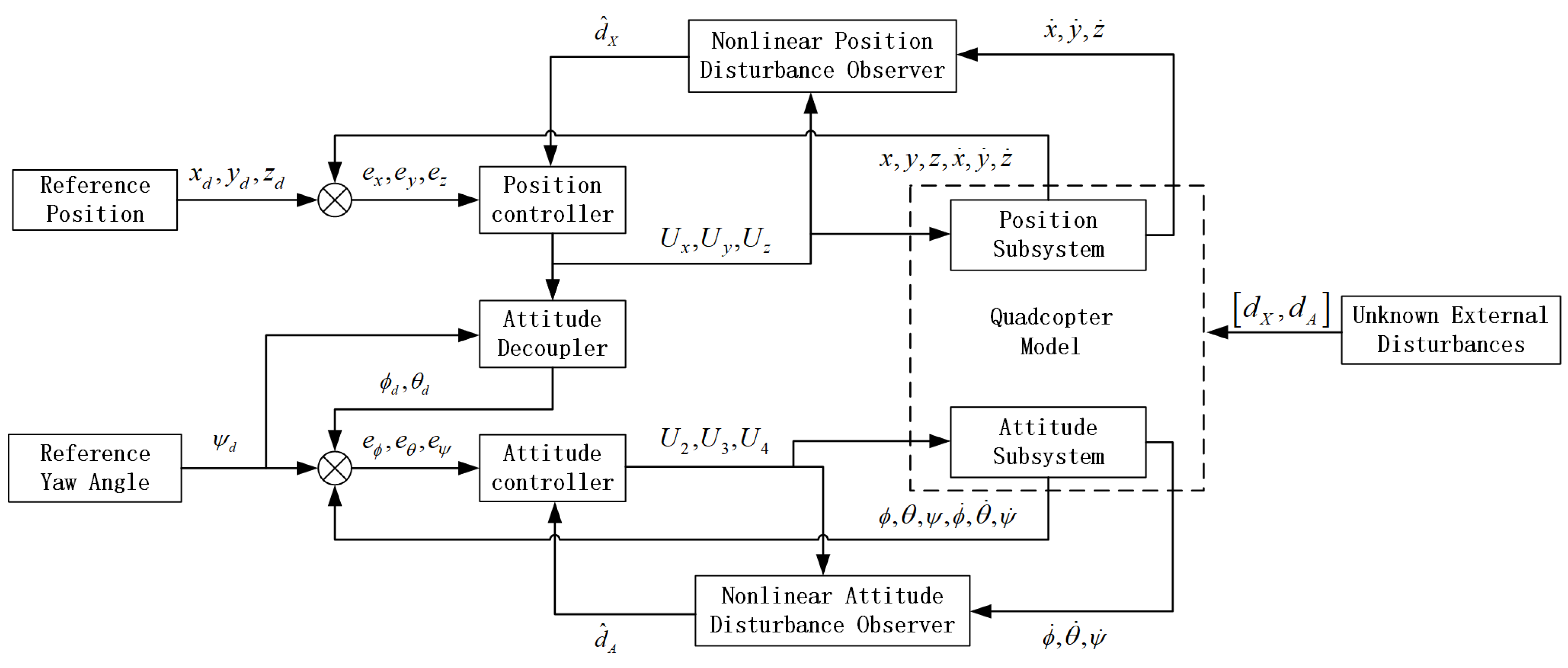
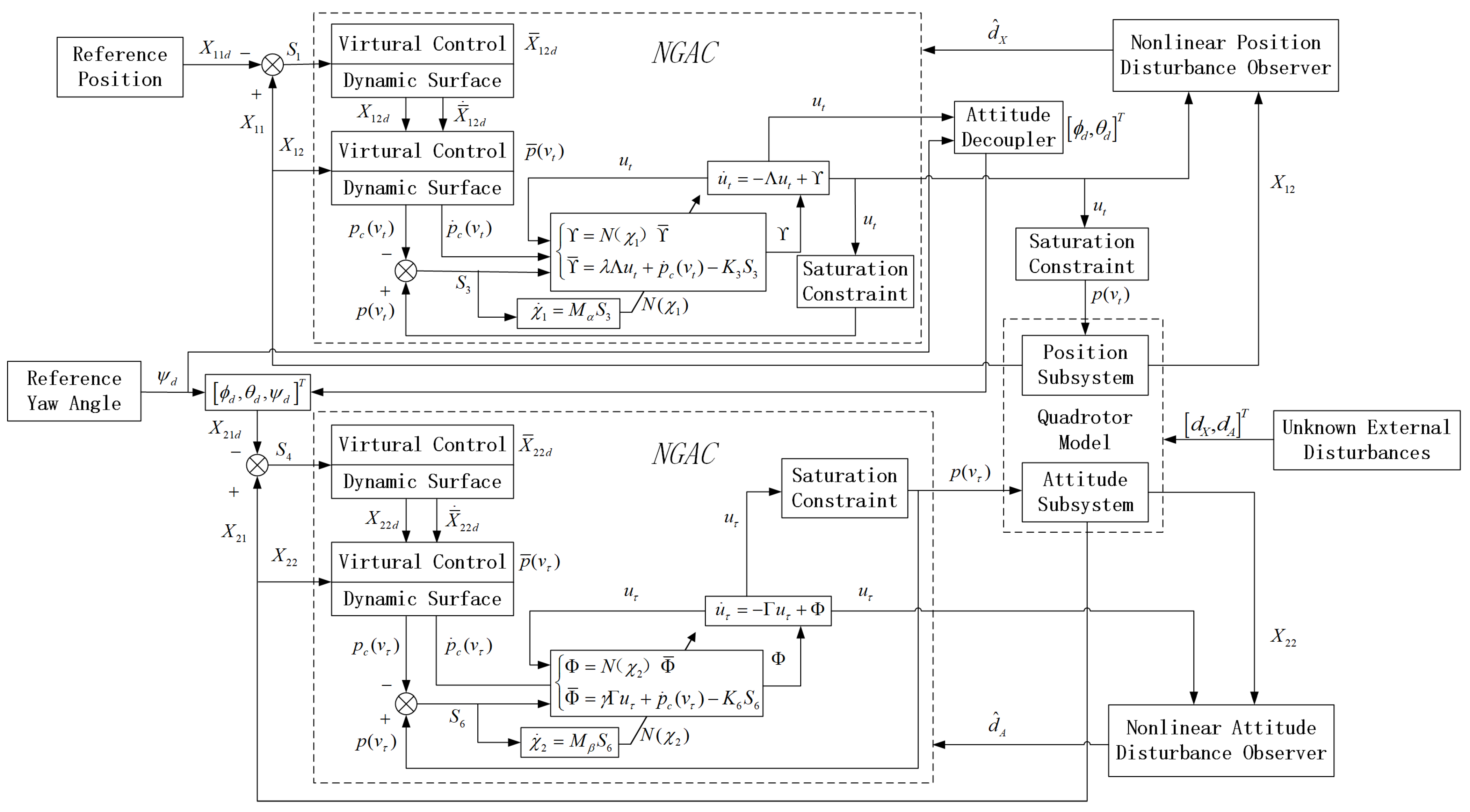
The subsequent sections of this paper are organized as follows: Section 2 describes the modeling of the quadrotor UAV. Section 3 outlines the design of the nonlinear disturbance observer and the controllers for position and attitude. Section 4 provides a stability analysis of the proposed controller. Section 5 presents the simulation results and analysis, and finally, Section 6 concludes with some remarks on the findings.

2. Materials and Methods

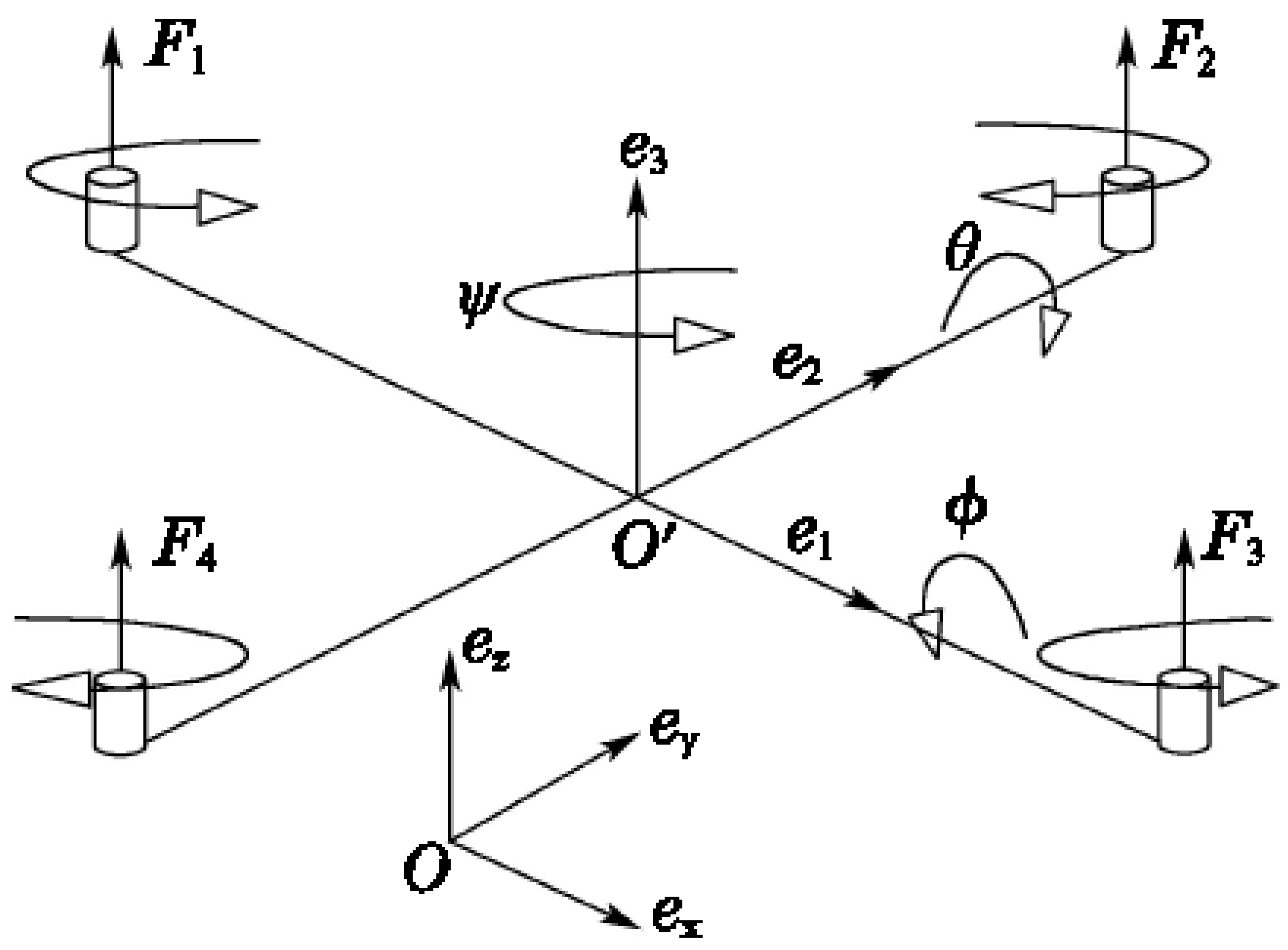
As depicted in Figure 1, disregarding the Earth’s rotation, a specific location on the Earth’s surface is chosen as the origin to establish an inertial coordinate system $(e_x,e_y,e_z)$. The center of the starting bracket O is selected as the reference point, and the geometric center of the airframe is taken as the origin to define the airframe coordinate system $(e_1,e_2,e_3)$. The transformation from the airframe coordinate system to the inertial coordinate system can be achieved through coordinate system rotation. The position vector $(x,y,z)$ of the quadrotor is defined within the inertial coordinate system, whereas the attitude vector $(\varphi ,\theta ,\psi )$, composed of roll, pitch, and yaw angles, is defined under the airframe coordinate system. The dynamic model of the quadrotor is decoupled into two subsystems: position and attitude.

The position dynamic subsystem is described as

$$\begin{array}{c}\hfill \left\{\begin{array}{c}{\dot{X}}_{11}=X_{12}\hfill \\ {\dot{X}}_{12}=u_t-z_{e}g-D_1{X}_{12}+d_X\hfill \end{array}\right.\end{array}$$

(1)

where $X_{11}={[x,y,z]}^T$ is the vehicle position vector, $X_{12}={[\dot{x},\dot{y},\dot{z}]}^T$ is the linear velocity vector of the vehicle in the inertial coordinate system, $z_e={(0,0,1)}^T$ is a space vector in the inertial coordinate system, g is the acceleration due to gravity, and $d_X={[d_1,d_2,d_3]}^T$ represent external unknown disturbances of the position subsystem. The $u_t={[u_x,u_y,u_z]}^T$ denote the control quantities in the $x,y,z$ directions, $D_1{X}_{12}$ represent the internal uncertain disturbance, and $u_t$ and $D_1{X}_{12}$ can be expressed as

$$\begin{array}{c}\hfill u_t=\left[\begin{array}{c}\hfill (\cos \varphi \sin \theta \cos \psi +\sin \varphi \sin \psi )U_1\hfill \\ \hfill (\cos \varphi \sin \theta \sin \psi -\sin \varphi \cos \psi )U_1\hfill \\ \hfill \left(\cos \varphi \cos \theta \right)U_1\hfill \end{array}\right],D_1{X}_{12}=\left[\begin{array}{c}{d}_x\dot{x}/m\hfill \\ d_y\dot{y}/m\hfill \\ d_z\dot{z}/m\hfill \end{array}\right].\hfill \end{array}$$

(2)

where $(d_x,d_y,d_z)$ is the air-damping coefficient, m is the mass of the quadrotor, and $U_1$ is the total lift generated by the four rotors.

The attitude dynamic subsystem is described as follows

$$\begin{array}{c}\hfill \left\{\begin{array}{c}{\dot{X}}_{21}=X_{22}\hfill \\ {\dot{X}}_{22}=u_{\tau }-D_2{X}_{22}-\Theta -\mathrm{H}+d_A\hfill \end{array}\right.\end{array}$$

(3)

where $X_{21}={[\varphi ,\theta ,\psi ]}^T$ is the vehicle angle vector, $X_{22}={[\dot{\varphi },\dot{\theta },\dot{\psi }]}^T$ is the vehicle angular velocity vector in the inertial coordinate system, and $u_{\tau }={[U_2,U_3,U_4]}^T$ is the airframe input moment vector, which represents the torques of roll, pitch, and yaw angles. $d_A={[d_4,d_5,d_6]}^T$ is an unknown external disturbance, and $D_2{X}_{22}$, $\Theta$, and $\mathrm{H}$ can be described as

$$\begin{array}{c}\hfill D_2{X}_{22}=\left[\begin{array}{c}{d}_{\varphi }\dot{\varphi }/J_x\hfill \\ d_{\theta }\dot{\theta }/J_y\hfill \\ d_{\psi }\dot{\psi }/J_z\hfill \end{array}\right],\Theta =\left[\begin{array}{c}(J_y-J_z)\dot{\theta }\dot{\psi }/J_x\hfill \\ (J_z-J_x)\dot{\varphi }\dot{\psi }/J_y\hfill \\ (J_x-J_y)\dot{\varphi }\dot{\theta }/J_z\hfill \end{array}\right],\mathrm{H}=\left[\begin{array}{c}{J}_r\dot{\theta }/J_x\hfill \\ J_r\dot{\varphi }/J_y\hfill \\ 0\hfill \end{array}\right].\end{array}$$

(4)

where $(d_{\varphi },d_{\theta },d_{\psi })$ are the corresponding air resistance coefficients, $(J_x,J_y,J_z)$ are the moment of inertia of the quadrotor in X, Y, and Z axes, respectively, and $J_r$ is the moment of inertia of the four rotors.

In summary, the dynamic model of a quadrotor [27,28] can be formulated as follows:

$$\begin{array}{c}\hfill \left\{\begin{array}{c}\ddot{x}=(C_{\varphi }{S}_{\theta }{C}_{\psi }+S_{\varphi }{S}_{\psi })U_1-a_1\dot{x}+d_1\hfill \\ \ddot{y}=(C_{\varphi }{S}_{\theta }{S}_{\psi }-S_{\varphi }{C}_{\psi })U_1-a_2\dot{y}+d_2\hfill \\ \ddot{z}=\left(C_{\varphi }{C}_{\theta }\right)U_1-g-a_3\dot{z}+d_3\hfill \\ \ddot{\varphi }=a_4\dot{\theta }\dot{\psi }+a_5\dot{\theta }-a_6\dot{\varphi }+U_2+d_4\hfill \\ \ddot{\theta }=a_7\dot{\varphi }\dot{\psi }+a_8\dot{\varphi }-a_9\dot{\theta }+U_3+d_5\hfill \\ \ddot{\psi }=a_{10}\dot{\varphi }\dot{\theta }-a_{11}\dot{\psi }+U_4+d_6\hfill \end{array}\right.\end{array}$$

(5)

where S and C denote $sin$ and $cos$, respectively, $a_i,i=1,2,\dots ,11$ are the internal parameters of the quadrotor system, the parameters are defined as:

$$\begin{array}{c}{a}_1=\frac{d_x}{m},a_2=\frac{d_y}{m},a_3=\frac{d_z}{m},a_4=\frac{J_y-J_z}{J_x},a_5=\frac{J_r}{J_x},a_6=\frac{d_{\varphi }}{J_x},\hfill \\ a_7=\frac{J_z-J_x}{J_y},a_8=\frac{J_r}{J_y},a_9=\frac{d_{\theta }}{J_y},a_{10}=\frac{J_x-J_y}{J_z},a_{11}=\frac{d_{\psi }}{J_z}.\hfill \end{array}$$

For the purpose of subsequent controller design and stability analysis, the following assumptions and definitions are made here:

Assumption A1.

The desired position $X_{11d}={[x_d,y_d,z_d]}^T$ and desired attitude $X_{21d}={[{\varphi }_d,{\theta }_d,{\psi }_d]}^T$ are continuously derivable, and their derivatives exist and are bounded. The ${\dot{X}}_{11d}$, ${\ddot{X}}_{11d}$,${\dot{X}}_{21d}$, and ${\ddot{X}}_{21d}$ exist. For the positive real numbers ${\sigma }_1$ and ${\sigma }_2$, the inequalities ${∥X_{11d}∥}^2+{∥{\dot{X}}_{11d}∥}^2+{∥{\ddot{X}}_{11d}∥}^2\le {\sigma }_1$ and ${∥X_{21d}∥}^2+{∥{\dot{X}}_{21d}∥}^2+{∥{\ddot{X}}_{21d}∥}^2\le {\sigma }_2$ hold.

Definition 1.

A function is called a Nussbaum-type function [29] if it has the following properties:

$$\begin{array}{c}\hfill \begin{array}{c}\underset{s\to \infty }{lim}sup{\int }_{s_0}^{s}N\left(\chi \right)d\chi =+\infty \hfill \\ \underset{s\to \infty }{lim}inf{\int }_{s_0}^{s}N\left(\chi \right)d\chi =-\infty \hfill \end{array}\end{array}$$

(6)

The Nussbaum function chosen for this paper is $N\left(\chi \right)={\chi }^2\cos \left(\chi \right)$.

Definition 2

([21]). Assume S be a subset of ${\mathbb{R}}^n$, and then the set S is called an open subset of ${\mathbb{R}}^n$, if for every χ in the set S, there exists $\epsilon >0$ makes $N(\chi ,\epsilon )=\{z\in {\mathbb{R}}^n:|z-\chi |<\epsilon \}$ is a subset of S. A set S is called closed if and only if the complementary set of S in ${\mathbb{R}}^n$ is open. If there exists $r>0$ makes $\left|\chi \right|<r$ holds for all $\chi \in S$, we call the set S bounded.

Then, if and only if a set S is closed and bounded, we call the set S compact.

Definition 3

([30]). For the system $\dot{\chi }=f(t,\chi )$, where $f:[0,\infty )\times D\to {\mathbb{R}}^n$ is piecewise continuous in t and locally Lipschitz in χ on $[0,\infty )\times D$, and $D\subset {\mathbb{R}}^n$ is a domain, which contains the origin. If $\forall \varsigma >0$, there is $\delta (t_0,\varsigma )>0$, which makes

$$\begin{array}{c}\hfill |\chi \left(t_0\right)|\le \delta (t_0,\varsigma )\Rightarrow \left|\chi (t;{\chi }_0,t_0)\right|\le \varsigma ,\forall t\ge t_0.\end{array}$$

(7)

Then the system is semiglobal stable.

Lemma 1

([24]). Let V(·) and χ(·) be smooth functions defined on $[0,t_f)$ with $V\left(t\right)\ge 0$, $\forall t\in [0,t_f)$. For $t\in [0,t_f)$, if the following inequality holds:

$$\begin{array}{c}\hfill V\left(t\right)\le c_0+e^{-c_{1}t}{\int }_0^t\left[\kappa \right(\tau \left)N\right(\chi )-1]\dot{\chi }{e}^{c_{1}t}d\tau \end{array}$$

(8)

where the constant $c_1>0$, $\kappa \left(\tau \right)$ is a time-varying parameter which takes a value in the intervals $I:=(0,1]$, and $c_0$ denotes some appropriate positive constant, then $V\left(t\right),\chi \left(t\right)$ and ${\int }_0^t\kappa \left(\tau \right)N\left(\chi \right)\dot{\chi }d\tau$ must be bounded on $[0,t_f)$.

In this paper, the control goal is to design an adaptive trajectory tracking strategy, given any desired trajectory $X_{11d}$ and yaw angle ${\psi }_d$ that satisfy Assumption 1, combined with the dynamic surface control technique, enabling the quadrotor to track the given desired trajectory and ensuring the closed-loop system is stable and linear as well as the boundedness of the system state signals.

3. Controller Design

In this paper, an adaptive dynamic surface control scheme based on the Nussbaum function is proposed to decompose the quadrotor system into two dynamic subsystems, position subsystems and attitude subsystems, and design the controllers separately. The design scheme is shown in Figure 2.

3.1. Design of Nonlinear Disturbance Observer

In this subsection, a nonlinear disturbance observer for the quadrotor system is first designed, divided into two parts: the position disturbance observer and the attitude disturbance observer.

3.1.1. Design of a Position Disturbance Observer

In order to estimate the unknown disturbances of the positioning subsystem, the design nonlinear disturbance observer [31] of the form (1) as

$$\begin{array}{c}\hfill \left\{\begin{array}{c}{\dot{p}}_X=-L_X{p}_X-L_X[L_X{X}_{12}-u_t-z_{e}g-D_1{X}_{12}]\hfill \\ {\widehat{d}}_X=p_X+L_X{X}_{12}\hfill \end{array}\right.\end{array}$$

(9)

where $L_X=diag\left\{[l_x,l_y,l_z]\right\}$, $l_x,l_y,l_z>0$ are designed gain matrix parameters, $p_X={[p_x,p_y,p_z]}^T$ is the internal state, and ${\widehat{d}}_X={[{\widehat{d}}_1,{\widehat{d}}_2,{\widehat{d}}_3]}^T$ is the estimate of the external disturbances.

3.1.2. Design of an Attitude Disturbance Observer

Similarly, in order to estimate the unknown disturbances of the attitude subsystem design the nonlinear disturbance observer [32] of (3) as:

$$\begin{array}{c}\hfill \left\{\begin{array}{c}{\dot{p}}_A=-L_A{p}_A-L_A[L_A{X}_{22}-u_{\tau }-\Theta -\mathrm{H}-D_2{X}_{22}]\hfill \\ {\widehat{d}}_A=p_A+L_A{X}_{22}\hfill \end{array}\right.\end{array}$$

(10)

where $L_A=diag\left\{[l_{\varphi },l_{\theta },l_{\psi }]\right\}$ is the gain matrix, and $l_{\varphi },l_{\theta },l_{\psi }>0$, $p_A={[p_{\varphi },p_{\theta },p_{\psi }]}^T$ is the internal state, and ${\widehat{d}}_A={[{\widehat{d}}_4,{\widehat{d}}_5,{\widehat{d}}_6]}^T$ is the estimate of the external disturbances.

3.2. Design of Position and Attitude Controllers

In this subsection, we will design the controllers for both the position and attitude subsystems of the quadrotor. First, we will design the controller for the position subsystem; then, based on the output of the position subsystem controller, we will derive the desired roll, pitch, and total lift. Finally, we will proceed with the design of the attitude subsystem.

3.2.1. Design of Position Controller

When designing the controller, input saturation [26] problem is considered and $u_t$ is replaced by the saturation function $Sat\left(v_t\right)=Sa{t}_{u_{t_M}}\left(u_t\right)$, the saturation function is defined as

$$\begin{array}{c}\hfill Sat\left(v_t\right)=\left\{\begin{array}{c}{u}_{tM},u_t⩾u_{tM}\hfill \\ u_t,-u_{tM}<u_t<u_{tM}\hfill \\ -u_{tM},u_t⩽-u_{tM}\hfill \end{array}\right.\end{array}$$

(11)

where $u_{tM}$ is the upper input limit of the quadrotor. The saturation function defined by (11) is not differentiable everywhere within its domain. To ensure that the designed backstepping control strategy can be implemented, the hyperbolic tangent function is introduced to replace the saturation function, ensuring that ut is differentiable everywhere within its domain; its form [25] can be expressed as

$$\begin{array}{c}\hfill p\left(v_t\right)=u_{tM}tanh\frac{u_t}{u_{tM}}\end{array}$$

(12)

Particularly, for the convenience of obtaining the control law, an augmented position subsystem [33] is introduced as

$$\begin{array}{c}\hfill \left\{\begin{array}{c}{\dot{X}}_{11}=X_{12}\hfill \\ {\dot{X}}_{12}=p\left(v_t\right)-z_{e}g-D_1{X}_{12}+d_X\hfill \\ {\dot{u}}_t=-\Lambda u_t+{\rm Y}\hfill \end{array}\right.\end{array}$$

(13)

where $\Lambda =diag\left([{\Lambda }_1,{\Lambda }_2,{\Lambda }_3]\right)$ denotes the gain matrix and the parameters ${\Lambda }_1,{\Lambda }_2,{\Lambda }_3>0$, ${\rm Y}$ is an auxiliary variable.

With this, the preparatory work is concluded, and below are the detailed design steps for the position subsystem controller.

Step 1: Set the first error surface $S_1$, and the derivation of $S_1$ yields

$$\begin{array}{c}\hfill S_1=X_{11}-X_{11d}\end{array}$$

(14)

$$\begin{array}{c}\hfill {\dot{S}}_1=X_{12}-{\dot{X}}_{11d}\end{array}$$

(15)

Set the virtual control input ${\overline{X}}_{12d}$ as

$$\begin{array}{c}\hfill {\overline{X}}_{12d}=-K_1{S}_1+{\dot{X}}_{11d}\end{array}$$

(16)

where $K_1=diag\left([k_{11},k_{12},k_{13}]\right),k_{11},k_{12},k_{13}>0$ are the parameters to be designed. Let $X_{12d}$ be the output of ${\overline{X}}_{12d}$ through the low-pass filter

$$\begin{array}{c}\hfill \left\{\begin{array}{c}{T}_1{\dot{X}}_{12d}+X_{12d}={\overline{X}}_{12d}\hfill \\ X_{12d}\left(0\right)={\overline{X}}_{12d}\left(0\right)\hfill \end{array}\right.\end{array}$$

(17)

where $T_1$ is the time constant, the initial values of $X_{12d}$ and ${\overline{X}}_{12d}$ are equal. Then, the filter error $y_1$ and filter ${\dot{X}}_{12d}$ can be expressed as

$$\begin{array}{c}\hfill y_1=X_{12d}-{\overline{X}}_{12d}\end{array}$$

(18)

$$\begin{array}{c}\hfill {\dot{X}}_{12d}=T_1^{-1}({\overline{X}}_{12d}-X_{12d})=-T_1^{-1}{y}_1\end{array}$$

(19)

Step 2: Set the first error surface $S_2$, and the derivation of $S_2$ yields

$$\begin{array}{c}\hfill S_2=X_{12}-X_{12d}\end{array}$$

(20)

$$\begin{array}{c}\hfill {\dot{S}}_2=p\left(v_t\right)-z_{e}g-D_1{X}_{12}+d_X-{\dot{X}}_{12d}\end{array}$$

(21)

Set the virtual control law $\overline{p}\left(v_t\right)$ as

$$\begin{array}{c}\hfill \overline{p}\left(v_t\right)={\dot{X}}_{12d}+z_{e}g+D_1{X}_{12}-{\widehat{d}}_X-K_2{S}_2\end{array}$$

(22)

where $K_2=diag\left([k_{21},k_{22},k_{23}]\right)$ is a positive diagonal constant matrix, ${\widehat{d}}_X$ is the observed value from the disturbance observer, serving as compensation for the controller. Let $p_c\left(v_t\right)$ be the output of $\overline{p}\left(v_t\right)$ through the low-pass filter

$$\begin{array}{c}\hfill \left\{\begin{array}{c}{T}_2{\dot{p}}_c\left(v_t\right)+p_c\left(v_t\right)=\overline{p}\left(v_t\right)\hfill \\ p_c\left(v_t\right)\left(0\right)=\overline{p}\left(v_t\right)\left(0\right)\hfill \end{array}\right.\end{array}$$

(23)

where $T_2$ is the time constant, the initial values of $p_c\left(v_t\right)$ and $\overline{p}\left(v_t\right)$ are equal. Then, the filter error $y_2$ and filter ${\dot{p}}_c\left(v_t\right)$ can be expressed as

$$\begin{array}{c}\hfill y_2=p_c\left(v_t\right)-\overline{p}\left(v_t\right)\end{array}$$

(24)

$$\begin{array}{c}\hfill {\dot{p}}_c\left(v_t\right)=T_2^{-1}(\overline{p}\left(v_t\right)-p_c\left(v_t\right))=-T_2^{-1}{y}_2\end{array}$$

(25)

Step 3: Set the third error surface $S_3$, and differentiating $S_3$ yields

$$\begin{array}{c}\hfill S_3=p\left(v_t\right)-p_c\left(v_t\right)\end{array}$$

(26)

$$\begin{array}{c}\hfill {\dot{S}}_3=\lambda (-\Lambda u_t+{\rm Y})-{\dot{p}}_c\left(v_t\right)\end{array}$$

(27)

where $\lambda =\partial p\left(v_t\right)/\partial u_t=diag\left([{\lambda }_1,{\lambda }_2,{\lambda }_3]\right)$ is a time-varying matrix and its elements are within $(0,1]$. For system stability, the auxiliary variable ${\rm Y}$ is designed as

$$\begin{array}{c}\hfill \left\{\begin{array}{c}{\rm Y}=N\left({\chi }_1\right)\overline{{\rm Y}}\hfill \\ \overline{{\rm Y}}=\lambda \Lambda u_t+{\dot{p}}_c\left(v_t\right)-K_3{S}_3\hfill \end{array}\right.\end{array}$$

(28)

where $K_3=diag\left([k_{31},k_{32},k_{33}]\right)$ is a positive constant matrix. The adjustment parameters ${\chi }_1={[{\chi }_{11},{\chi }_{12},{\chi }_{13}]}^T$ and Nussbaum gain $N\left({\chi }_1\right)=diag\left([N\left({\chi }_{11}\right),N\left({\chi }_{12}\right),N\left({\chi }_{13}\right)]\right)$ is introduced to deal with the time-varying $\lambda$ with an adaptive law as

$$\begin{array}{c}\hfill {\dot{\chi }}_1=M_{\alpha }{S}_3\end{array}$$

(29)

where $M_{\alpha }=diag\left([{\alpha }_1{\overline{{\rm Y}}}_1,{\alpha }_2{\overline{{\rm Y}}}_2,{\alpha }_3{\overline{{\rm Y}}}_3]\right)$, and ${\alpha }_1,{\alpha }_2,{\alpha }_3>0$ are designed parameters.

3.2.2. Design of Attitude Decoupler

Through the previous subsection, we have obtained $u_t$. In this subsection, we design an attitude decoupler to solve for the desired roll and pitch angles of the quadrotor, and thus, we define it as follows:

$$\begin{array}{c}\hfill \left\{\begin{array}{c}{U}_x=(\cos \varphi \sin \theta \cos \psi +\sin \varphi \sin \psi )U_1\hfill \\ U_y=(\cos \varphi \sin \theta \sin \psi -\sin \varphi \cos \psi )U_1\hfill \\ U_z=\left(\cos \varphi \cos \theta \right)U_1\hfill \end{array}\right.\end{array}$$

(30)

According to (30), the desired yaw angle in the formula is known, multiplying the first equation in (30) by $\cos {\psi }_d$, plus the second equation in (30) by $\sin {\psi }_d$ and combining the third equation in (30) to obtain the desired pitch angle. Similarly, multiplying the first equation in (30) by $\sin {\psi }_d$ minus the second equation in (30) by $\cos {\psi }_d$ and combining the third equation in (30) to obtain the desired roll angle. Finally, the total lift is obtained through the third equation in (30). The desired roll(${\varphi }_d$) and pitch(${\theta }_d$) angle and the total lift [34] can be expressed as following:

$$\begin{array}{c}\hfill \left\{\begin{array}{c}{\theta }_d=arctan\left(\frac{U_x\cos {\psi }_d+U_y\sin {\psi }_d}{U_z}\right)\hfill \\ {\varphi }_d=arctan\left(\cos {\theta }_d\frac{U_x\sin {\psi }_d-U_y\cos {\psi }_d}{U_z}\right)\hfill \\ U_1=\frac{U_z}{\cos {\varphi }_d\cos {\theta }_d}\hfill \end{array}\right.\end{array}$$

(31)

3.2.3. Design of Attitude Controller

While designing the controller, the input saturation [26] problem is considered and $u_{\tau }$ is replaced by the saturation function $Sat\left(v_{\tau }\right)=Sa{t}_{u_{{\tau }_M}}\left(u_{\tau }\right)$; the saturation function is defined as

$$\begin{array}{c}\hfill Sat\left(v_{\tau }\right)=\left\{\begin{array}{c}{u}_{\tau M},u_{\tau }⩾u_{\tau M}\hfill \\ u_{\tau },-u_{\tau M}<u_{\tau }<u_{\tau M}\hfill \\ -u_{\tau M},u_{\tau }⩽-u_{\tau M}\hfill \end{array}\right.\end{array}$$

(32)

where $u_{\tau M}$ is the upper input limit of the quadrotor. Similarly, to ensure that ut is differentiable everywhere within its domain, the hyperbolic tangent function is introduced to replace the saturation function; the form [25] can be expressed as

$$\begin{array}{c}\hfill p\left(v_{\tau }\right)=u_{\tau M}tanh\frac{u_{\tau }}{u_{\tau M}}\end{array}$$

(33)

Particularly, in order to facilitate the acquisition of control laws, an augmented attitude subsystem [33] is introduced and the system is rewritten as

$$\begin{array}{c}\hfill \left\{\begin{array}{c}{\dot{X}}_{21}=X_{22}\hfill \\ {\dot{X}}_{22}=p\left(v_{\tau }\right)-D_2{X}_{22}-\Theta -\mathrm{H}+d_A\hfill \\ {\dot{u}}_{\tau }=-\Gamma u_{\tau }+\Phi \hfill \end{array}\right.\end{array}$$

(34)

where $\Gamma =diag\left([{\Gamma }_1,{\Gamma }_2,{\Gamma }_3]\right)$ is gain matrix and the parameters ${\Gamma }_1,{\Gamma }_2,{\Gamma }_3>0$, $\Phi$ is an auxiliary variable.

At this point, the preparatory phase is complete and the subsequent steps detail the design process for the attitude subsystem controller.

Step 1: Set the first error surface $S_4$ and obtain the derivative

$$\begin{array}{c}\hfill S_4=X_{21}-X_{21d}\end{array}$$

(35)

$$\begin{array}{c}\hfill {\dot{S}}_4=X_{22}-{\dot{X}}_{21d}\end{array}$$

(36)

Set the virtual control input ${\overline{X}}_{22d}$ as

$$\begin{array}{c}\hfill {\overline{X}}_{22d}=-K_4{S}_4+{\dot{X}}_{21d}\end{array}$$

(37)

where $K_4=diag\left([k_{41},k_{42},k_{43}]\right)$ and $k_{41},k_{42},k_{43}>0$ are designed parameters. Let $X_{22d}$ be the output of ${\overline{X}}_{22d}$ through the low-pass filter

$$\begin{array}{c}\hfill \left\{\begin{array}{c}{T}_3{\dot{X}}_{22d}+X_{22d}={\overline{X}}_{22d}\hfill \\ X_{22d}\left(0\right)={\overline{X}}_{22d}\left(0\right)\hfill \end{array}\right.\end{array}$$

(38)

where $T_3$ is the time constant, the initial values of $X_{22d}$ and ${\overline{X}}_{22d}$ are equal. Then, the filter error $y_3$ and filter ${\dot{X}}_{22d}$ can be expressed as

$$\begin{array}{c}\hfill y_3=X_{22d}-{\overline{X}}_{22d}\end{array}$$

(39)

$$\begin{array}{c}\hfill {\dot{X}}_{22d}=T_3^{-1}({\overline{X}}_{22d}-X_{22d})=-T_3^{-1}{y}_3\end{array}$$

(40)

Step 2: Set the second error surface $S_5$ and obtain the derivative

$$\begin{array}{c}\hfill S_5=X_{22}-X_{22d}\end{array}$$

(41)

$$\begin{array}{c}\hfill {\dot{S}}_5=p\left(v_{\tau }\right)-D_2{X}_{22}-\Theta -\mathrm{H}+d_A-{\dot{X}}_{22d}\end{array}$$

(42)

Let the virtual control law $\overline{p}\left(v_{\tau }\right)$ be:

$$\begin{array}{c}\hfill \overline{p}\left(v_{\tau }\right)={\dot{X}}_{22d}+D_2{X}_{22}+\Theta +\mathrm{H}-{\widehat{d}}_A-K_5{S}_5\end{array}$$

(43)

where $K_5=diag\left([k_{51},k_{52},k_{53}]\right)$, $k_{51},k_{52},k_{53}>0$ are designed parameters and ${\widehat{d}}_A$ is the observed value from the disturbance observer, serving as compensation for the controller. Let $p_c\left(v_{\tau }\right)$ be the output of $\overline{p}\left(v_{\tau }\right)$ through the low-pass filter

$$\begin{array}{c}\hfill \left\{\begin{array}{c}{T}_4{\overline{p}}_c\left(v_{\tau }\right)+p_c\left(v_{\tau }\right)=\overline{p}\left(v_{\tau }\right)\hfill \\ p_c\left(v_{\tau }\right)\left(0\right)=\overline{p}\left(v_{\tau }\right)\left(0\right)\hfill \end{array}\right.\end{array}$$

(44)

where $T_4$ is the time constant, the initial values of $p_c\left(v_{\tau }\right)$ and $\overline{p}\left(v_{\tau }\right)$ are equal. Then, the filter error $y_4$ and filter ${\dot{p}}_c\left(v_{\tau }\right)$ can be expressed as

$$\begin{array}{c}\hfill y_4=p_c\left(v_{\tau }\right)-\overline{p}\left(v_{\tau }\right)\end{array}$$

(45)

$$\begin{array}{c}\hfill {\dot{p}}_c\left(v_{\tau }\right)=T_4^{-1}(\overline{p}\left(v_{\tau }\right)-p_c\left(v_{\tau }\right))=-T_4^{-1}{y}_4\end{array}$$

(46)

Step 3: Set the third error surface $S_6$ and obtain the derivative

$$\begin{array}{c}\hfill S_6=p\left(v_{\tau }\right)-p_c\left(v_{\tau }\right)\end{array}$$

(47)

$$\begin{array}{c}\hfill {\dot{S}}_6=\gamma (-\Gamma u_{\tau }+\Phi )-{\dot{p}}_c\left(v_{\tau }\right)\end{array}$$

(48)

where $\gamma =\partial p\left(v_{\tau }\right)/\partial u_{\tau }=diag\left([{\gamma }_1,{\gamma }_2,{\gamma }_3]\right)$ is a time-varying matrix, and its elements are within $(0,1]$. For stabilizing the system, the auxiliary variable $\Phi$ is designed as

$$\begin{array}{c}\hfill \left\{\begin{array}{c}\Phi =N\left({\chi }_2\right)\overline{\Phi }\hfill \\ \overline{\Phi }=\gamma \Gamma u_{\tau }+{\dot{p}}_c\left(v_{\tau }\right)-K_6{S}_6\hfill \end{array}\right.\end{array}$$

(49)

where $K_6=diag\left([k_{61},k_{62},k_{63}]\right)$ is a positive constant matrix. The adjustment parameters ${\chi }_2={[{\chi }_{21},{\chi }_{22},{\chi }_{23}]}^T$ and the Nussbaum gain $N\left({\chi }_2\right)=diag\left([N\left({\chi }_{21}\right),N\left({\chi }_{22}\right),N\left({\chi }_{23}\right)]\right)$ is introduced to deal with the time-varying $\gamma$ with an adaptive law as

$$\begin{array}{c}\hfill {\dot{\chi }}_2=M_{\beta }{S}_6\end{array}$$

(50)

where $M_{\beta }=diag\left([{\beta }_1{\overline{\Phi }}_1,{\beta }_2{\overline{\Phi }}_2,{\beta }_3{\overline{\Phi }}_3]\right)$, and ${\beta }_1,{\beta }_2,{\beta }_3>0$ are designed parameters.

The above control scheme is shown in Figure 3 below.

4. Stability Analysis

In this section, a stability analysis is conducted on the provided control scheme to ensure that all signals in both the position and attitude subsystems are ultimately bounded.

From (15), (16), (18), and (20), we have

$$\begin{array}{cc}\hfill {\dot{S}}_1& =X_{12}-{\dot{X}}_{11d}\hfill \\ \hfill & =(X_{12}-X_{12d})+(X_{12d}-{\overline{X}}_{12d})+({\overline{X}}_{12d}-{\dot{X}}_{11d})\hfill \\ \hfill & =S_2+y_1-K_1{S}_1\hfill \end{array}$$

(51)

Invoking (21), (22), (24), and (26) to obtain

$$\begin{array}{cc}\hfill {\dot{S}}_2& =p\left(v_t\right)-z_{e}g-D_1{X}_{12}+d_X-{\dot{X}}_{12d}\hfill \\ \hfill & =(p\left(v_t\right)-p_c\left(v_t\right))+(p_c\left(v_t\right)-\overline{p}\left(v_t\right))+(\overline{p}\left(v_t\right)-z_{e}g-D_1{X}_{12}+d_X-{\dot{X}}_{12d})\hfill \\ \hfill & =S_3+y_2-K_2{S}_2\hfill \end{array}$$

(52)

Combine (27) and (28) to obtain

$$\begin{array}{cc}\hfill {\dot{S}}_3& =\lambda (-\Lambda u_t+{\rm Y})-{\dot{p}}_c\left(v_t\right)\hfill \\ \hfill & =\lambda (-\Lambda u_t+{\rm Y})-\overline{{\rm Y}}+\overline{{\rm Y}}-{\dot{p}}_c\left(v_t\right)\hfill \\ \hfill & =-\lambda \Lambda u_t+(\lambda N\left({\chi }_1\right)\overline{{\rm Y}}-\overline{{\rm Y}})+(\lambda \Lambda u_t+{\dot{p}}_c\left(v_t\right)-K_3{S}_3)-{\dot{p}}_c\left(v_t\right)\hfill \\ \hfill & =(\lambda N\left({\chi }_1\right)-I)\overline{{\rm Y}}-K_3{S}_3\hfill \end{array}$$

(53)

Calling formulas (36), (37), (39), and (41) can gain

$$\begin{array}{cc}\hfill {\dot{S}}_4& =X_{22}-{\dot{X}}_{21d}\hfill \\ \hfill & =(X_{22}-X_{22d})+(X_{22d}-{\overline{X}}_{22d})+({\overline{X}}_{22d}-{\dot{X}}_{21d})\hfill \\ \hfill & =S_5+y_3-K_4{S}_4\hfill \end{array}$$

(54)

Refer to Equation (42) and consider (43), (45), and (47) to obtain

$$\begin{array}{cc}\hfill {\dot{S}}_5& =p\left(v_{\tau }\right)-D_2{X}_{22}-\Theta -\mathrm{H}+d_A-{\dot{X}}_{22d}\hfill \\ \hfill & =(p\left(v_{\tau }\right)-p_c\left(v_{\tau }\right))+(p_c\left(v_{\tau }\right)-\overline{p}\left(v_{\tau }\right))+(\overline{p}\left(v_{\tau }\right)-D_2{X}_{22}-\Theta -\mathrm{H}+d_A-{\dot{X}}_{22d})\hfill \\ \hfill & =S_6+y_4-K_5{S}_5\hfill \end{array}$$

(55)

Based on (48) and (49), we have

$$\begin{array}{cc}\hfill {\dot{S}}_6& =\gamma (-\Gamma u_{\tau }+\Phi )-{\dot{p}}_c\left(v_{\tau }\right)\hfill \\ \hfill & =\gamma (-\Gamma u_{\tau }+\Phi )-\overline{\Phi }+\overline{\Phi }-{\dot{p}}_c\left(v_{\tau }\right)\hfill \\ \hfill & =-\gamma \Gamma u_t+\left(\gamma N\left({\chi }_2\right)\overline{\Phi }\right)-\overline{\Phi }+(\gamma \Gamma u_{\tau }+{\dot{p}}_c\left(v_{\tau }\right)-K_6{S}_6)-{\dot{p}}_c\left(v_{\tau }\right)\hfill \\ \hfill & =(\gamma N\left({\chi }_2\right)-I)\overline{\Phi }-K_6{S}_6\hfill \end{array}$$

(56)

Differentiating $y_1$ in (18) and using (16), (19), and (51), this yields

$$\begin{array}{c}\hfill {\dot{y}}_1=-T_1^{-1}{y}_1+{\eta }_1\end{array}$$

(57)

where ${\eta }_1$ is a function of $S_1,S_2,y_1,X_{11d},{\dot{X}}_{11d},{\ddot{X}}_{11d}$ and has the following form:

$$\begin{array}{c}\hfill {\eta }_1=K_1(S_2+y_1-K_1{S}_1)-{\ddot{X}}_{11d}\end{array}$$

(58)

Differentiating $y_2$ in (24) and using (22), (25), and (52), we have

$$\begin{array}{c}\hfill {\dot{y}}_2=-T_2^{-1}{y}_2+{\eta }_2\end{array}$$

(59)

where ${\eta }_2$ is a function of $S_1,S_2,S_3,y_1,y_2,X_{11d},{\dot{X}}_{11d},{\ddot{X}}_{11d}$ and has the following form:

$$\begin{array}{c}\hfill {\eta }_2=K_2(S_3+y_2-K_2{S}_2)-(D_1{\dot{X}}_{12d}+{\ddot{X}}_{12d}+z_e\dot{g}-{\widehat{d}}_X)\end{array}$$

(60)

Differentiating $y_3$ in (39) and using (37), (40), and (54), we can obtain

$$\begin{array}{c}\hfill {\dot{y}}_3=-T_3^{-1}{y}_3+{\eta }_3\end{array}$$

(61)

where ${\eta }_3$ is a function of $S_4,S_5,y_3,X_{21d},{\dot{X}}_{21d},{\ddot{X}}_{21d}$ and has the following form:

$$\begin{array}{c}\hfill {\eta }_3=K_4(S_5+y_3-K_4{S}_4)-{\ddot{X}}_{21d}\end{array}$$

(62)

Differentiating $y_4$ in (45), and using (43), (46), and (55), we obtain

$$\begin{array}{c}\hfill {\dot{y}}_4=-T_4^{-1}{y}_4+{\eta }_4\end{array}$$

(63)

where ${\eta }_4$ is a function of $S_4,S_5,S_6,y_3,y_4,X_{21d},{\dot{X}}_{21d},{\ddot{X}}_{21d}$ and has the following form:

$$\begin{array}{c}\hfill {\eta }_4=K_5(S_6+y_4-K_5{S}_5)-(\Theta +\mathrm{H}+D_2{\dot{X}}_{22d}+{\ddot{X}}_{22d}-{\widehat{d}}_A)\end{array}$$

(64)

The Lyapunov function for the entire system is constructed as follows:

$$\begin{array}{c}\hfill V=V_1+V_2+V_3+V_4\end{array}$$

(65)

where $V_1$ and $V_2$ are the Lyapunov functions for the position subsystem, and similarly, $V_3$ and $V_4$ are the Lyapunov functions for the attitude subsystem, represented as follows:

$$\begin{array}{c}\hfill V_1=\frac{1}{2}{S}_1^T{S}_1+\frac{1}{2}{S}_2^T{S}_2+\frac{1}{2}{S}_3^T{S}_3\end{array}$$

(66)

$$\begin{array}{c}\hfill V_2=\frac{1}{2}{y}_1^T{y}_1+\frac{1}{2}{y}_2^T{y}_2\end{array}$$

(67)

$$\begin{array}{c}\hfill V_3=\frac{1}{2}{S}_4^T{S}_4+\frac{1}{2}{S}_5^T{S}_5+\frac{1}{2}{S}_6^T{S}_6\end{array}$$

(68)

$$\begin{array}{c}\hfill V_4=\frac{1}{2}{y}_3^T{y}_3+\frac{1}{2}{y}_4^T{y}_4\end{array}$$

(69)

Theorem 1.

Consider a closed-loop system expanded by position subsystem (13) and attitude subsystem (34). The semi-global stability of the closed-loop system is ensured with appropriate design parameters with the initial condition $V\left(0\right)\le \mu ,\mu >0$ holding, the error of position tracking $∥e_{X_{11}}∥=∥S_1∥$ and the error of attitude tracking $∥e_{X_{21}}∥=∥S_4∥$ converging with arbitrarily small errors, and the control inputs, states, and all closed-loop system signals being bounded.

Proof. 

Based on (51)–(53) and (66), differentiating $V_1$ yields

$$\begin{array}{cc}\hfill {\dot{V}}_1& =S_1^T{\dot{S}}_1+S_2^T{\dot{S}}_2+S_3^T{\dot{S}}_3\hfill \\ \hfill & \le ∥S_1∥∥S_2∥+∥S_1∥∥y_1∥-{\rho }_1{S}_1^T{S}_1+∥S_2∥∥S_3∥+∥S_2∥∥y_2∥\hfill \\ \hfill & -{\rho }_2{S}_2^T{S}_2+S_3^T(\lambda N\left({\chi }_1\right)-I)\overline{{\rm Y}}-{\rho }_3{S}_3^T{S}_3\hfill \end{array}$$

(70)

In a similar way, from (54)–(56) and (68), to take the derivative of $V_3$

$$\begin{array}{cc}\hfill {\dot{V}}_3& =S_4^T{\dot{S}}_4+S_5^T{\dot{S}}_5+S_6^T{\dot{S}}_6\hfill \\ \hfill & \le ∥S_4∥∥S_5∥+∥S_4∥∥y_3∥-{\rho }_4{S}_4^T{S}_4+∥S_5∥∥S_6∥+∥S_5∥∥y_4∥\hfill \\ \hfill & -{\rho }_5{S}_5^T{S}_5+S_6^T(\gamma N\left({\chi }_2\right)-I)\overline{\Phi }-{\rho }_6{S}_6^T{S}_6\hfill \end{array}$$

(71)

where ${\rho }_i(i=1,2,3,4,5,6)$ denotes the smallest eigenvalue of $K_i(i=1,2,3,4,5,6)$. Define a collection:

$$\begin{array}{c}\hfill {\Omega }_1=\{(X_{11d},{\dot{X}}_{11d},{\ddot{X}}_{11d}):{∥X_{11d}∥}^2+{∥{\dot{X}}_{11d}∥}^2+{∥{\ddot{X}}_{11d}∥}^2\le {\sigma }_1\}\end{array}$$

(72)

From Definition 2 and Assumption 1, one has that ${\Omega }_1$ is a compact set on ${\mathbb{R}}^3$. Consider two compact sets:

$$\begin{array}{c}\hfill {\Omega }_2=\{(S_1,S_2,y_1):\sum _{i=1}^2{∥S_i∥}^2+{∥y_1∥}^2\le 2{\mu }_1\}\end{array}$$

(73)

$$\begin{array}{c}\hfill {\Omega }_3=\{(S_1,S_2,S_3,y_1,y_2):\sum _{i=1}^3{∥S_i∥}^2+\sum _{i=1}^2{∥y_i∥}^2\le 2{\mu }_1\}\end{array}$$

(74)

Therefore, ${\Omega }_1\times {\Omega }_2$ is a compact set on ${\mathbb{R}}^6$ and ${\Omega }_1\times {\Omega }_3$ is a compact set on ${\mathbb{R}}^8$. Furthermore, ${\eta }_1,{\eta }_2$ are bounded on ${\Omega }_1\times {\Omega }_2$ and ${\Omega }_1\times {\Omega }_3$, respectively. Then, there must exist positive constants $M_1,M_2$ that satisfy $∥{\eta }_1∥\le M_1,∥{\eta }_2∥\le M_2$. Then, define another collection:

$$\begin{array}{c}\hfill {\Omega }_4=\{(X_{21d},{\dot{X}}_{21d},{\ddot{X}}_{21d}):{∥X_{21d}∥}^2+{∥{\dot{X}}_{21d}∥}^2+{∥{\ddot{X}}_{21d}∥}^2\le {\sigma }_2\}\end{array}$$

(75)

From Definition 2 and Assumption 1, one has that ${\Omega }_4$ is a compact set on ${\mathbb{R}}^3$. Consider two compact sets:

$$\begin{array}{c}\hfill {\Omega }_5=\{(S_4,S_5,y_3):\sum _{i=4}^5{∥S_i∥}^2+{∥y_3∥}^2\le 2{\mu }_2\}\end{array}$$

(76)

$$\begin{array}{c}\hfill {\Omega }_6=\{(S_4,S_5,S_6,y_3,y_4):\sum _{i=4}^6{∥S_i∥}^2+\sum _{i=3}^4{∥y_i∥}^2\le 2{\mu }_2\}\end{array}$$

(77)

Therefore, ${\Omega }_4\times {\Omega }_5$ is a compact set on ${\mathbb{R}}^6$ and ${\Omega }_4\times {\Omega }_6$ is a compact set on ${\mathbb{R}}^8$. Furthermore, ${\eta }_3,{\eta }_4$ are bounded on ${\Omega }_4\times {\Omega }_5$ and ${\Omega }_4\times {\Omega }_6$, respectively. Then, there must exist positive constants $M_3,M_4$ that satisfy $∥{\eta }_3∥\le M_3,∥{\eta }_4∥\le M_4$.

Invoking (57), (59), and (67) to derive $V_2$:

$$\begin{array}{cc}\hfill {\dot{V}}_2& =y_1^T{\dot{y}}_1+y_2^T{\dot{y}}_2\hfill \\ \hfill & \le -{\tau }_1^{-1}{y}_1^T{y}_1+∥y_1∥M_1-{\tau }_2^{-1}{y}_2^T{y}_2+∥y_2∥M_2\hfill \end{array}$$

(78)

Similarly, from (61), (63), and (69) to derive $V_4$:

$$\begin{array}{cc}\hfill {\dot{V}}_4& =y_3^T{\dot{y}}_3+y_4^T{\dot{y}}_4\hfill \\ \hfill & \le -{\tau }_3^{-1}{y}_3^T{y}_3+∥y_3∥M_3-{\tau }_4^{-1}{y}_4^T{y}_4+∥y_4∥M_4\hfill \end{array}$$

(79)

where ${\tau }_i^{-1}(i=1,2,3,4)$ denotes the smallest eigenvalue of $T_i^{-1}$. According to Young’s inequality and Theorem 1, the following time derivative can be obtained:

$$\begin{array}{cc}\hfill \dot{V}& \le -({\rho }_1-1)S_1^T{S}_1-({\rho }_2-3/2)S_2^T{S}_2-({\rho }_2-1/2)S_3^T{S}_3+S_3^T(\lambda N\left({\chi }_1\right)-I)\overline{{\rm Y}}\hfill \\ \hfill & -({\rho }_4-1)S_4^T{S}_4-({\rho }_5-3/2)S_5^T{S}_5-({\rho }_6-1/2)S_6^T{S}_6+S_6^T(\gamma N\left({\chi }_2\right)-I)\overline{\Phi }\hfill \\ \hfill & -({\tau }_1-1)y_1^T{y}_1-({\tau }_2-1)y_2^T{y}_2-({\tau }_3-1)y_3^T{y}_3-({\tau }_4-1)y_4^T{y}_4+(M_1^2+M_2^2+M_3^2+M_4^2)\hfill \\ \hfill & \le -2\rho V+S_3^T(\lambda N\left({\chi }_1\right)-I)\overline{{\rm Y}}+S_6^T(\gamma N\left({\chi }_2\right)-I)\overline{\Phi }+M\hfill \end{array}$$

(80)

where $\rho =min[{\rho }_1-1,{\rho }_2-3/2,{\rho }_3-1/2,{\rho }_4-1,{\rho }_5-3/2,{\rho }_6-1/2,{\tau }_1^{-1}-1,{\tau }_2^{-1}-1,{\tau }_3^{-1}-1,{\tau }_4^{-1}-1]$, and $M=\frac{1}{2}{\sum }_{i=1}^4{M}_i^2$.

For the stability of the closed-loop system, the relevant design parameters $K_i$$(i=1,2,3,4,5,6)$ and $T_i(i=1,2,3,4)$ should be chosen to make sure that ${\rho }_1-1>0$, ${\rho }_2-3/2>0,{\rho }_3-1/2>0,{\rho }_4-1>0,{\rho }_5-3/2>0,{\rho }_6-1/2>0,{\tau }_1^{-1}-1>0,{\tau }_2^{-1}-1>0$, ${\tau }_3^{-1}-1>0,{\tau }_4^{-1}-1>0$.

Thus, we can obtain:

$$\begin{array}{cc}\hfill V& \le V\left(0\right)e^{-2\rho t}+\frac{M}{2\rho }(1-e^{-2\rho t})\hfill \\ \hfill & +e^{-2\rho t}{\int }_0^t[{\dot{\chi }}_1^T{M}_{\alpha }^{-1}(\lambda N\left({\chi }_1\right)-I)\overline{{\rm Y}}+{\dot{\chi }}_2^T{M}_{\beta }^{-1}(\gamma N\left({\chi }_2\right)-I)\overline{\Phi }]e^{2\rho t}d\tau \hfill \end{array}$$

(81)

Invoking (28), (49) and noting that:

$$\begin{array}{cc}\hfill V_N& =e^{-2\rho t}{\int }_0^t[{\dot{\chi }}_1^T{M}_{\alpha }^{-1}(\lambda N\left({\chi }_1\right)-I)\overline{{\rm Y}}+{\dot{\chi }}_2^T{M}_{\beta }^{-1}(\gamma N\left({\chi }_2\right)-I)\overline{\Phi }]d\tau \hfill \\ \hfill & =\frac{e^{-2\rho t}}{{\alpha }_1}{\int }_0^t\left[({\lambda }_{1}N\left({\chi }_{11}\right)-1){\dot{\chi }}_{11}{e}^{2\rho t}\right]d\tau +\frac{e^{-2\rho t}}{{\alpha }_2}{\int }_0^t\left[({\lambda }_{2}N\left({\chi }_{12}\right)-1){\dot{\chi }}_{12}{e}^{2\rho t}\right]d\tau \hfill \\ \hfill & +\frac{e^{-2\rho t}}{{\alpha }_3}{\int }_0^t\left[({\lambda }_{3}N\left({\chi }_{13}\right)-1){\dot{\chi }}_{13}{e}^{2\rho t}\right]d\tau +\frac{e^{-2\rho t}}{{\beta }_1}{\int }_0^t\left[({\gamma }_{1}N\left({\chi }_{21}\right)-1){\dot{\chi }}_{21}{e}^{2\rho t}\right]d\tau \hfill \\ \hfill & +\frac{e^{-2\rho t}}{{\beta }_2}{\int }_0^t\left[({\gamma }_{2}N\left({\chi }_{22}\right)-1){\dot{\chi }}_{22}{e}^{2\rho t}\right]d\tau +\frac{e^{-2\rho t}}{{\beta }_3}{\int }_0^t\left[({\gamma }_{3}N\left({\chi }_{23}\right)-1){\dot{\chi }}_{23}{e}^{2\rho t}\right]d\tau \hfill \end{array}$$

(82)

From Lemma 1, we know $\chi ,{\int }_0^t[{\dot{\chi }}_1^T{M}_{\alpha }^{-1}(\lambda N\left({\chi }_1\right)-I)\overline{{\rm Y}}+{\dot{\chi }}_2^T{M}_{\beta }^{-1}(\gamma N\left({\chi }_2\right)-I)\overline{\Phi }]e^{2\rho t}d\tau$ and $V_N$ are bounded on $[0,t_f)$.

From the initial condition $V\left(0\right)\le \mu$ and (81), we can obtain that V is bounded on ${\Omega }_1\times {\Omega }_3\times {\Omega }_4\times {\Omega }_6$ and guarantees semi-global stability. Therefore, $S_1,S_2,S_3,S_4,S_5,S_6,y_1$, $y_2,y_3,y_4$ is bounded. In addition, the closed-loop system signal $X_{11d},X_{21d},{\overline{X}}_{12d},{\overline{X}}_{22d},\overline{p}\left(v_t\right)$, $\overline{p}\left(v_{\tau }\right)$ and the control input $u_t,u_{\tau }$ are bounded.

Define: $S={[S_1^T,S_2^T,S_3^T,S_4^T,S_5^T,S_6^T]}^T$, and

$$\begin{array}{c}\hfill {∥S∥}_{[0,T]}=\sqrt{\frac{1}{T}{\int }_0^T{S}^{T}Sdt}\end{array}$$

(83)

For integrating both sides of the inequality (80), one obtains:

$$\begin{array}{c}\hfill {∥S∥}_{[0,T]}\le \frac{1}{2\rho }\{\frac{V\left(T\right)+V\left(0\right)}{T}+M+\frac{1}{T}{\int }_0^T({\dot{\chi }}_1^T{M}_{\alpha }^{-1}\lambda N\left({\chi }_1\right)\overline{{\rm Y}}+{\dot{\chi }}_2^T{M}_{\beta }^{-1}\gamma N\left({\chi }_2\right)\overline{\Phi })dt\}\end{array}$$

(84)

Considering the inequalities on $[0,T]$, i.e., $e^{-2\rho T}\le 1,e^{-2\rho (T-t)}\le 1$ and $(1-e^{-2\rho T})/2\rho \le T$. Let $t=T$, from (81) we can have:

$$\begin{array}{c}\hfill \frac{V\left(T\right)+V\left(0\right)}{T}\le \frac{2V\left(0\right)}{T}+M+\frac{1}{T}{\int }_0^T({\dot{\chi }}_1^T{M}_{\alpha }^{-1}\lambda N\left({\chi }_1\right)\overline{{\rm Y}}+{\dot{\chi }}_2^T{M}_{\beta }^{-1}\gamma N\left({\chi }_2\right)\overline{\Phi })dt\end{array}$$

(85)

Noting that ${∥S_1∥}_{[0,T]}\le {∥S∥}_{[0,T]}$, and substituting (85) into (84) yields:

$$\begin{array}{c}\hfill {∥S_1∥}_{[0,T]}\le \frac{1}{\rho }\{\frac{V\left(0\right)}{T}+M+\frac{1}{T}{\int }_0^T({\dot{\chi }}_1^T{M}_{\alpha }^{-1}\lambda N\left({\chi }_1\right)\overline{{\rm Y}}+{\dot{\chi }}_2^T{M}_{\beta }^{-1}\gamma N\left({\chi }_2\right)\overline{\Phi })dt\}\end{array}$$

(86)

Then, the tracking errors of position and attitude are bounded and converge to arbitrarily small errors with suitable parameters. This is the end of the proof. □

5. Experimental Verification

In this section, the controllers designed above are validated. Section 5.1 presents the experimental platform related to the experiments, Section 5.2 displays the relevant parameters and initial states of the quadrotor for the semi-physical simulation experiments, Section 5.3 conducts experiments with the designed controllers and compares them with other controllers, and Section 5.4 shows the error analysis of the three controllers from Section 5.3.

5.1. Modeling Tech Experimental Platform

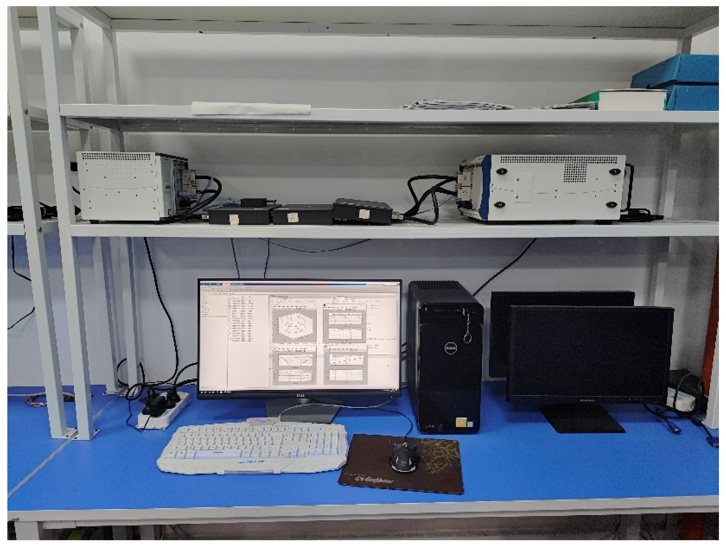
Through the StarSim Modeling Tech semi-physical simulation experiments of the traditional dynamic surface control (DSC), adaptive dynamic surface control based on the Nussbaum function (NGAC), and the control scheme of this paper (NGACDOB) are carried out by the real-time simulation experimental platform of power electronics. The hardware structure of the experimental platform is shown in Figure 4 and Figure 5.

The simulation results of the NGACDOB controller are shown as follows.

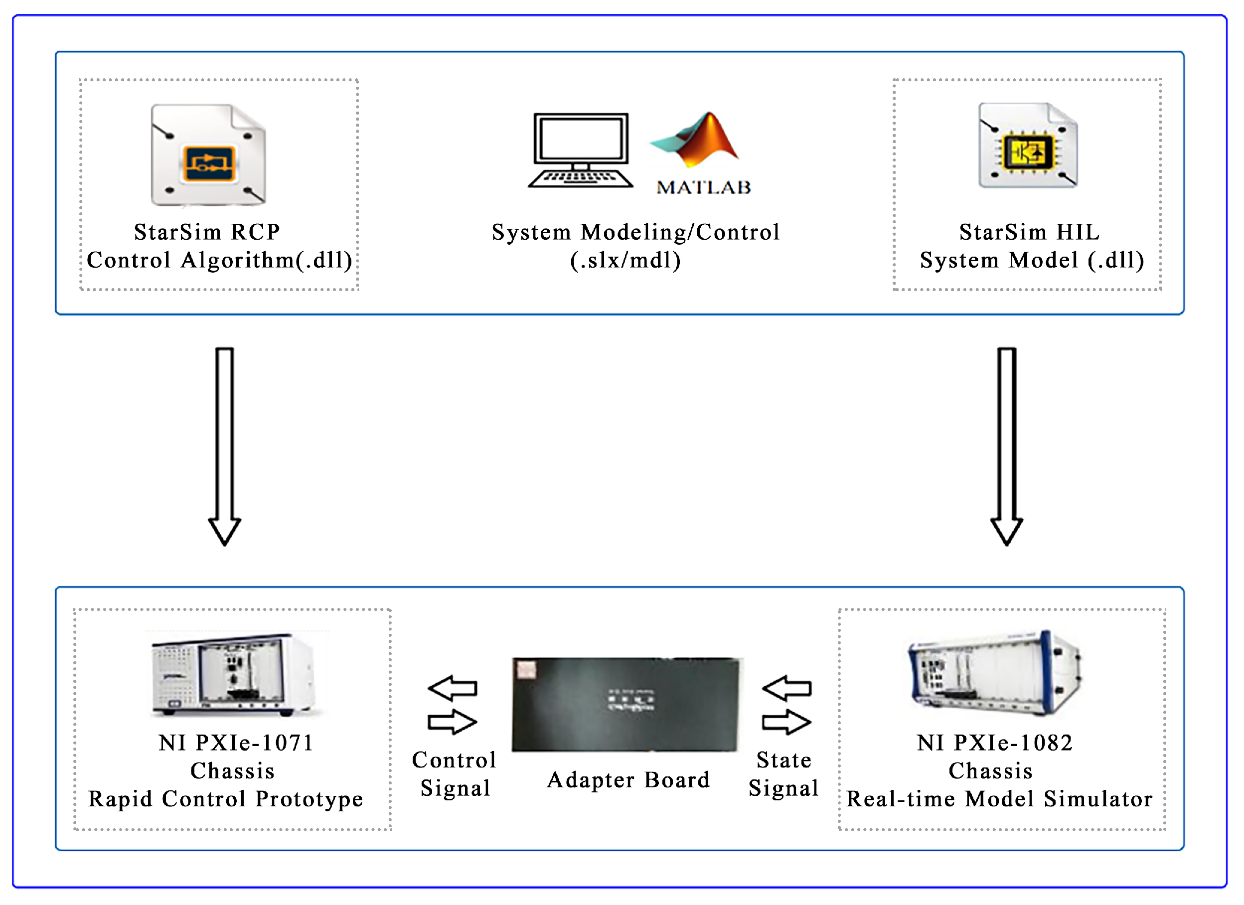
Experimental environment: (1) NI PXIe-1071, MTRCP (Rapid Control Prototype), the equipment adopts Kintex-7 325 T FPGA@Xilinx, and it has 16 analog input/output channels with a transmission rate of 1Ms/s. The device is used to run the proposed control algorithm in order to run the control code in real time and to run the control signals generated by the proposed control algorithm on the MT real-time simulator. (2) NIPXIe1082, the MT Real-Time Simulator (RTS) with a Kintex 7325T FPGA chip has 16-bit synchronous analog I/O channels and a data transfer rate of 1 MS/s. It is capable of performing FPGA simulations of large-scale power systems. The simulator receives the control signals, calculates the real-time response through the power electronics system, and outputs it to the control box. The RTS, RCP, and signal adapter form a closed-loop experimental system. (3) Experimental adapter board: used to connect signals between the control device and the model device. (4) Host: Matlab/Simulink system model and controller algorithms are downloaded to the Rapid Control Prototype and Real-Time Simulator, respectively, via Star SIM RCP software.

Remark 1.

It should be noted that the experimental validation in this paper is conducted on a semi-physical simulation platform, which is a real-time simulation technology that combines physical hardware with simulation software. This simulation method integrates physical components into the simulation loop of the system, allowing for a comprehensive examination and verification of system performance. The core feature of this method is embedding physical components into the simulation loop and requiring real-time operation, which solves the interface issues between the controller and the simulation computer, making the experimental results more realistic than pure mathematical simulation. The Modeling Tech experimental platform shown in Figure 4 runs the controller program, whereas the hardware structure of the experimental platform shown in Figure 5 runs the model program, with communication between the model and controller facilitated by a relay board. We aim to validate the control algorithm proposed in this paper through this semi-physical simulation experiment, laying the groundwork for physical experiments on flight vehicles.

5.2. Experimental Preparation

In order to verify the effectiveness of the control scheme proposed in this paper, a quadrotor with external perturbations and model uncertainties is considered, and the nominal parameters are shown in

Table 1. Quadrotor UAV main parameters.

Symbol	Value	Units	Symbol	Value	Units
m	1.4	kg	$d_x,d_y,d_z$	1	${10}^{-2} \mathrm{N}·{\mathrm{s}}^2·{\mathrm{rad}}^{-1}$
k	2.98	${10}^{-6} \mathrm{N}·{\mathrm{s}}^2·\mathrm{ra}{\mathrm{d}}^{-2}$	$d_{\varphi },d_{\theta },d_{\psi }$	0.5	${10}^{-2} \mathrm{N}·\mathrm{s}·{\mathrm{rad}}^{-1}$
l	0.2	m	$J_x$,$J_y$	1.25	$\mathrm{N}·{\mathrm{s}}^2·{\mathrm{ras}}^{-1}$
$J_r$	2.1	${10}^{-3} \mathrm{N}·{\mathrm{s}}^2·{\mathrm{rad}}^{-2}$	$J_z$	2.5	$\mathrm{N}·{\mathrm{s}}^2·{\mathrm{rad}}^{-1}$

.

The initial position is set as ($0,0,0.25$) and the initial attitude angle is ($0,0,0$). In order to accomplish the tracking target, the position controller parameters are selected as: $k_{11}=k_{12}=k_{13}=22$, $k_{21}=k_{22}=k_{23}=5,k_{31}=k_{32}=k_{33}=2,a_1=a_2=a_3=0.05$, ${\Lambda }_1={\Lambda }_2={\Lambda }_3=3,T_1=T_2=0.01,l_x=l_y=l_z=10$. The attitude controller parameters are selected as: $k_{41}=k_{42}=k_{43}=20,k_{51}=k_{52}=k_{53}=5,k_{61}=k_{62}=k_{63}=2$, $b_1=b_2=b_3=0.05,{\Gamma }_1={\Gamma }_2={\Gamma }_3=3,T_3=T_4=0.01,l_{\varphi }=l_{\theta }=l_{\psi }=10$. The reference trajectory of the quadrotor is $\left\{0.5\cos (0.5\mathrm{t}),0.5\sin (0.5\mathrm{t}),0.1\mathrm{t}\right\}$ and the desired yaw angle is $\pi /3$. Disturbances were added to the position and attitude subsystems at the 18th second, the duration of the disturbances lasted 1 s, and both position and attitude disturbances were $0.5\sin \left(\right(t-18\left)\pi \right)$. Then, disturbances were added to the position and attitude subsystems at the 25th second, the duration of the disturbances lasted 1 s, and both position and attitude disturbances were $-0.5\sin \left(\right(t-25\left)\pi \right)$.

5.3. Experimental Results

In this subsection, based on the experimental platform and the initial states and corresponding parameters of the model mentioned above, we will conduct three sets of experiments as follows: Experiment 1, Adaptive Dynamic Surface Control with Nussbaum Gain and Disturbance Observer (NGACDOB), Experiment 2, a comparative experiment between Traditional Dynamic Surface Control (DSC) and Adaptive Dynamic Surface Control with Nussbaum Gain and Disturbance Observer (NGACDOB), and Experiment 3, a comparative experiment between Adaptive Dynamic Surface Control based on Nussbaum Gain (NGAC) and Adaptive Dynamic Surface Control with Nussbaum Gain and Disturbance Observer (NGACDOB).

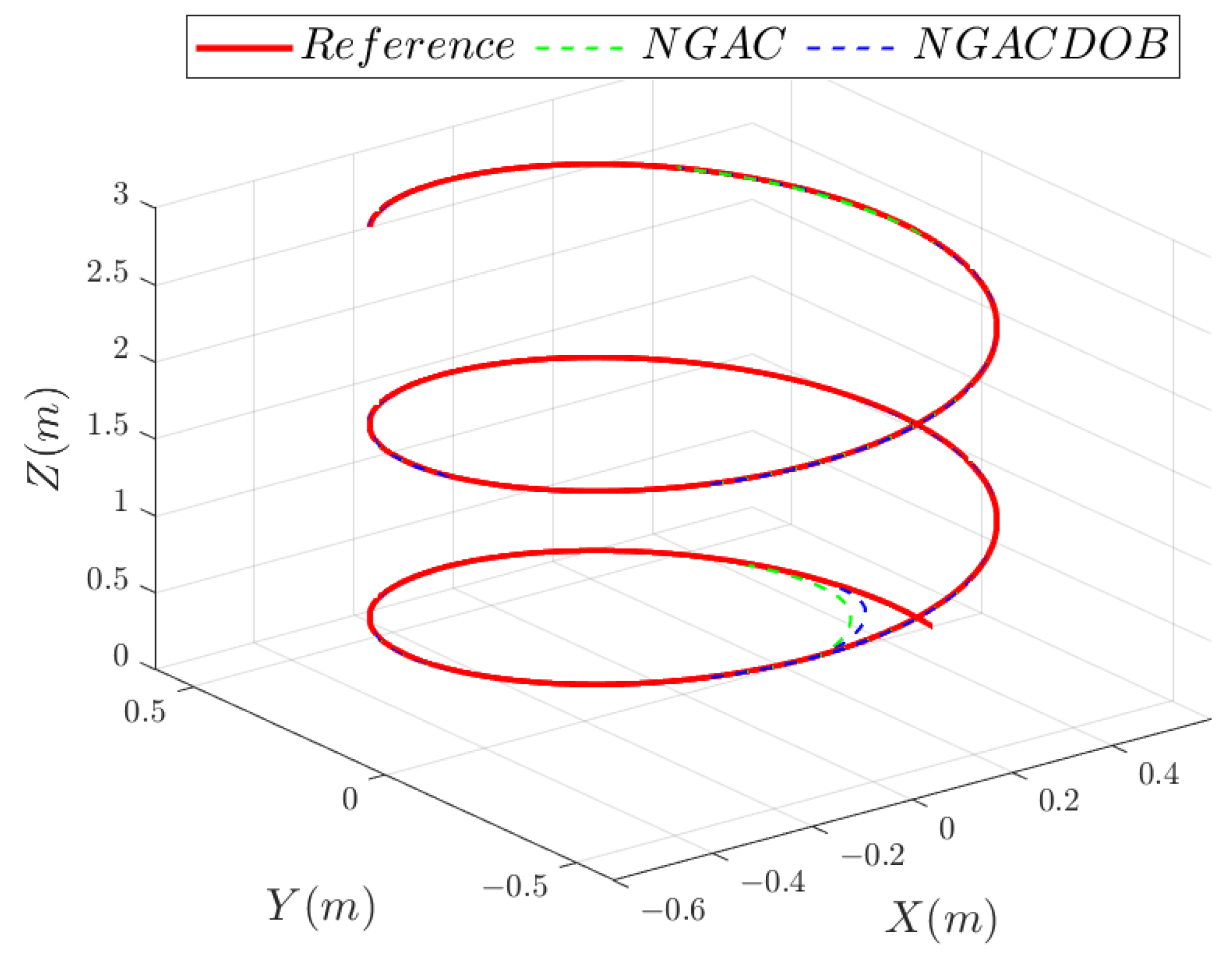
Experiment 1: The simulation results of NGACDOB

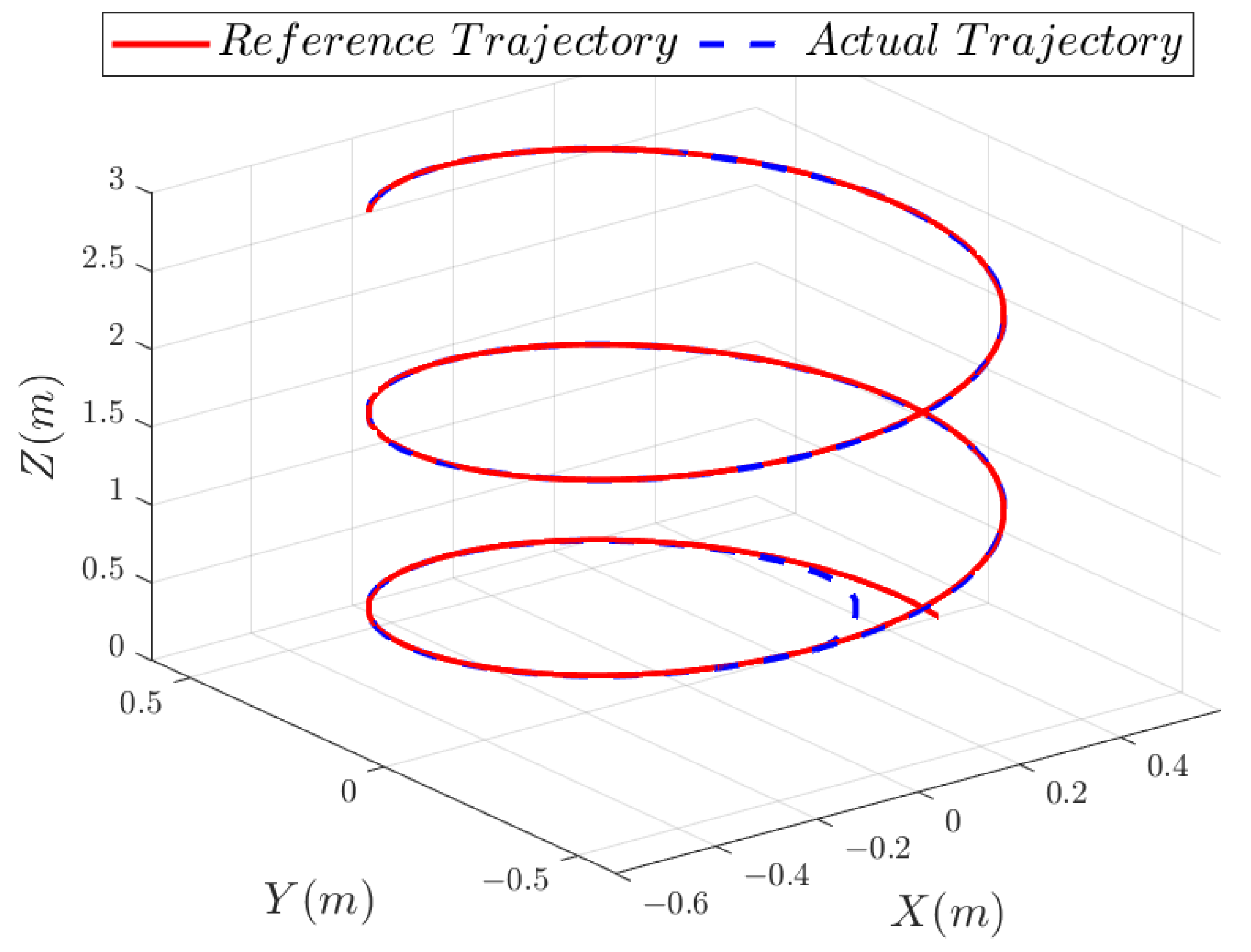
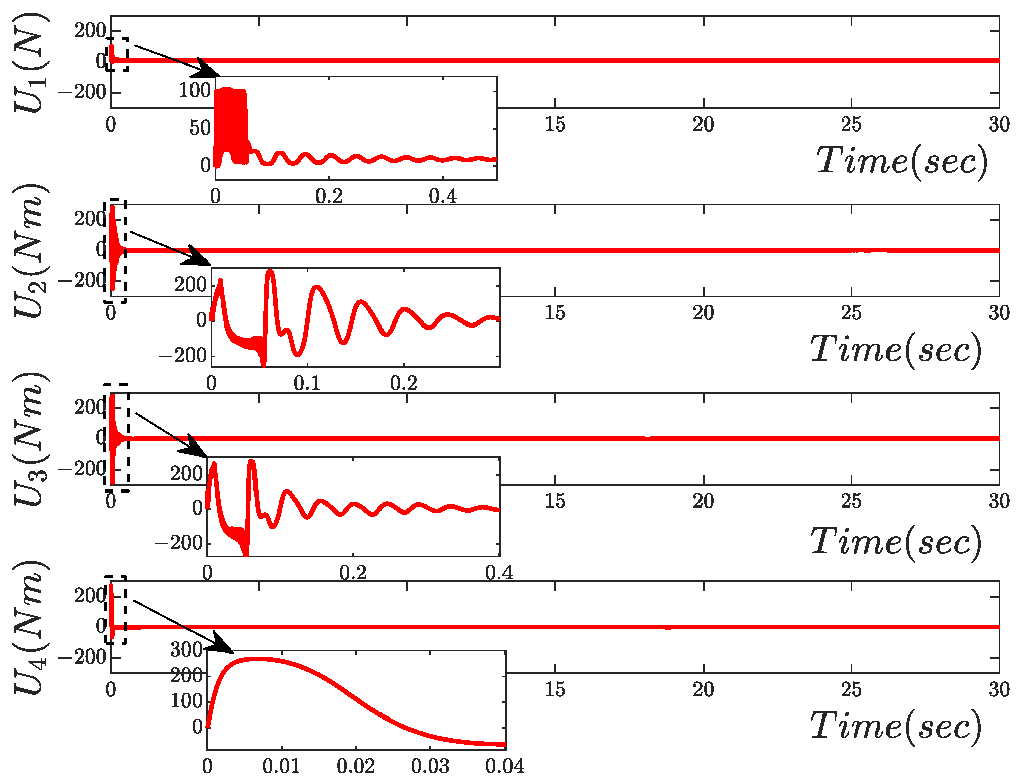
Figure 6 demonstrates the 3D tracking effect of the quadrotor, which follows a reference trajectory in the form of an ascending spiral during a 30 s simulation. It can be observed from the figure that the quadrotor is able to quickly track the reference trajectory. Figure 7 shows the changes in the input state of the quadrotor. Due to the introduction of input saturation in the controller design (Equations (12) and (33)), with the saturation values $u_{tM}$ and $u_{\tau M}$ both set to 300, the four input state values of the quadrotor are kept within 300 to prevent the input state values from being too high, which could result in the quadrotor’s actual lift and torque inputs from reaching the required conditions. The simulation results demonstrate the effectiveness of the input saturation control. 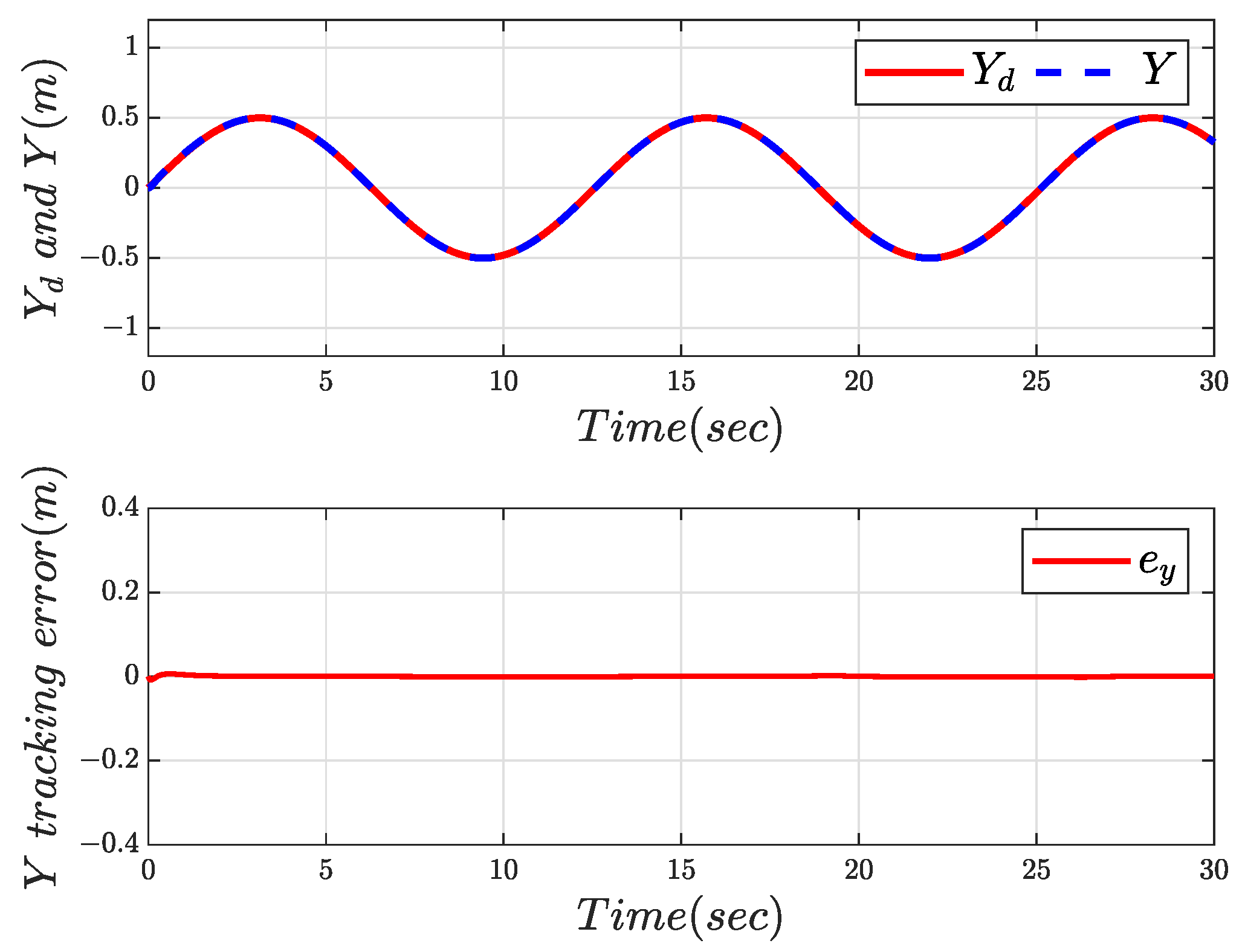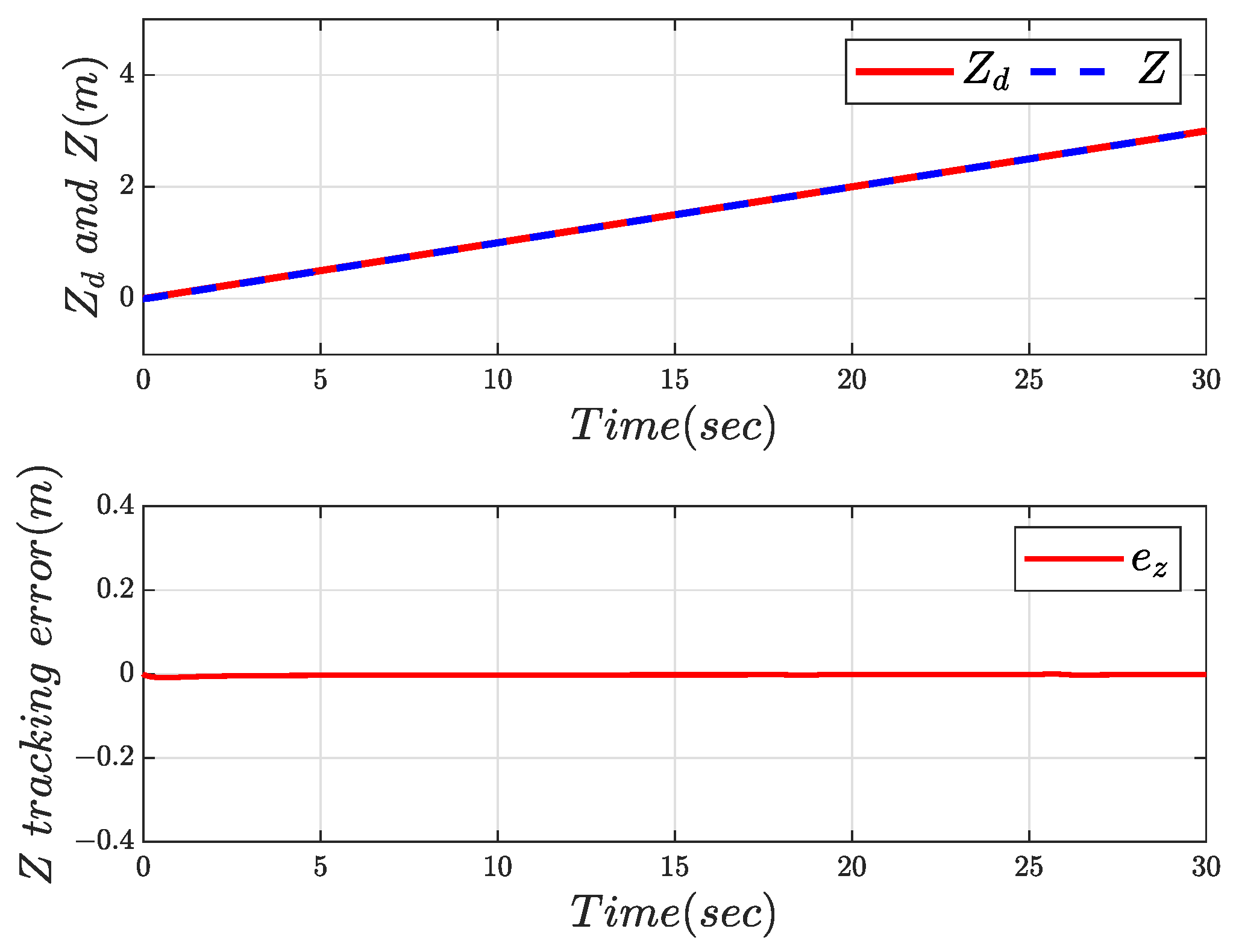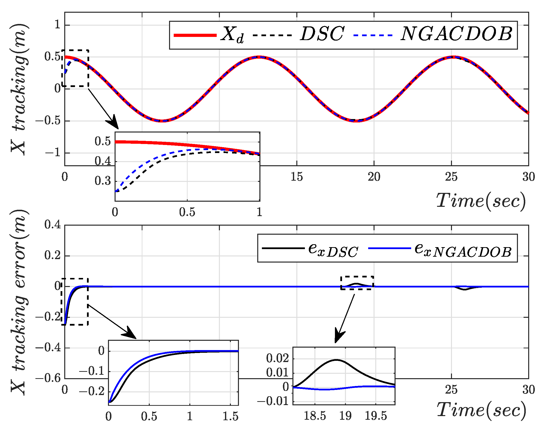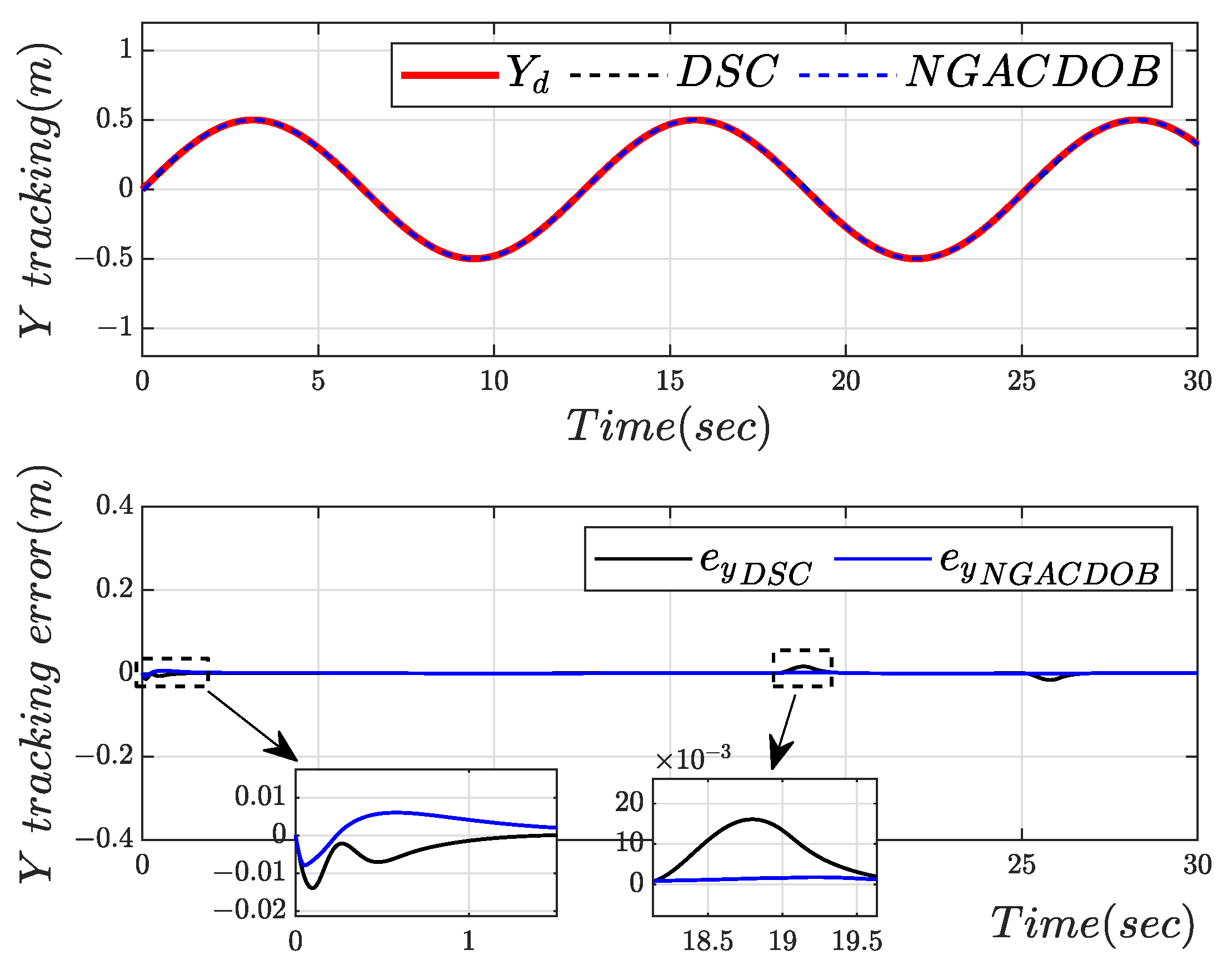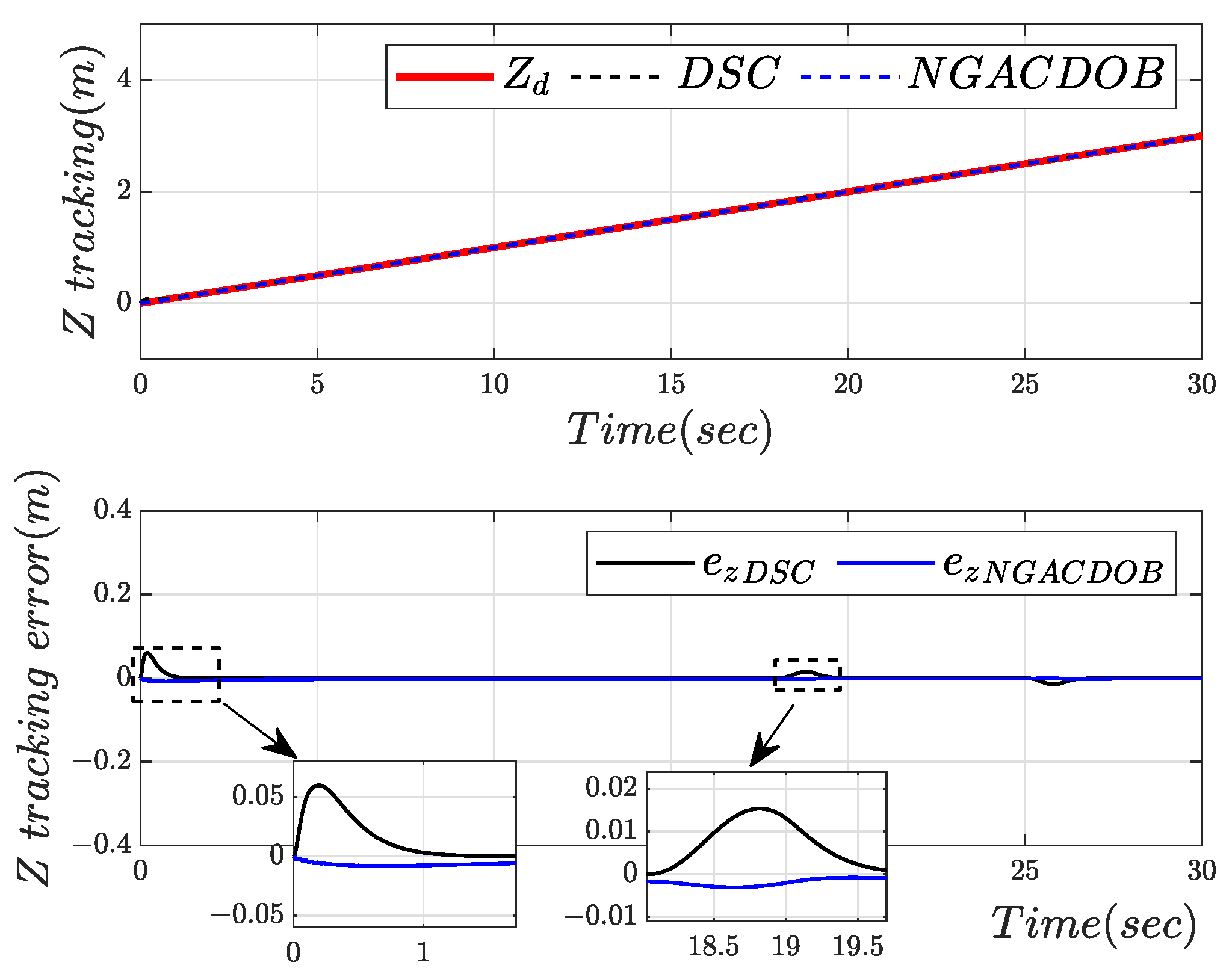Figure 8, Figure 9 and Figure 10 show the tracking and errors of the quadrotor in the X, Y, and Z directions. 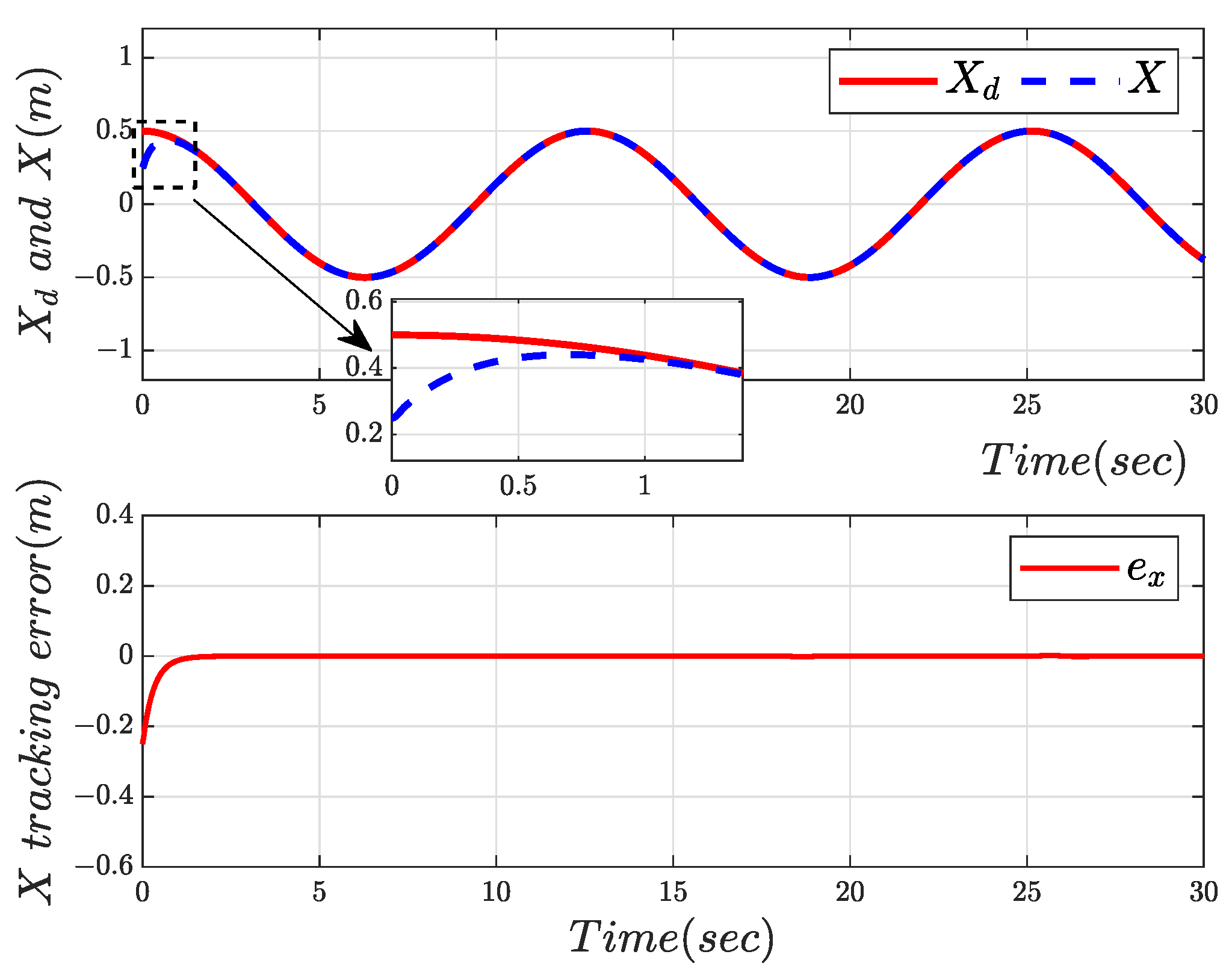To be realistic, the actual starting point is aligned with the reference trajectory’s starting point on the same horizontal plane, with only the initial value in the X direction being different; Figure 8 indicates that the aircraft tracks the reference signal after 0.6 s, and the tracking signals in all three directions show minimal fluctuations after disturbances at the 18th and 25th seconds, reflecting the effectiveness of the control algorithm and its good disturbance rejection capability. 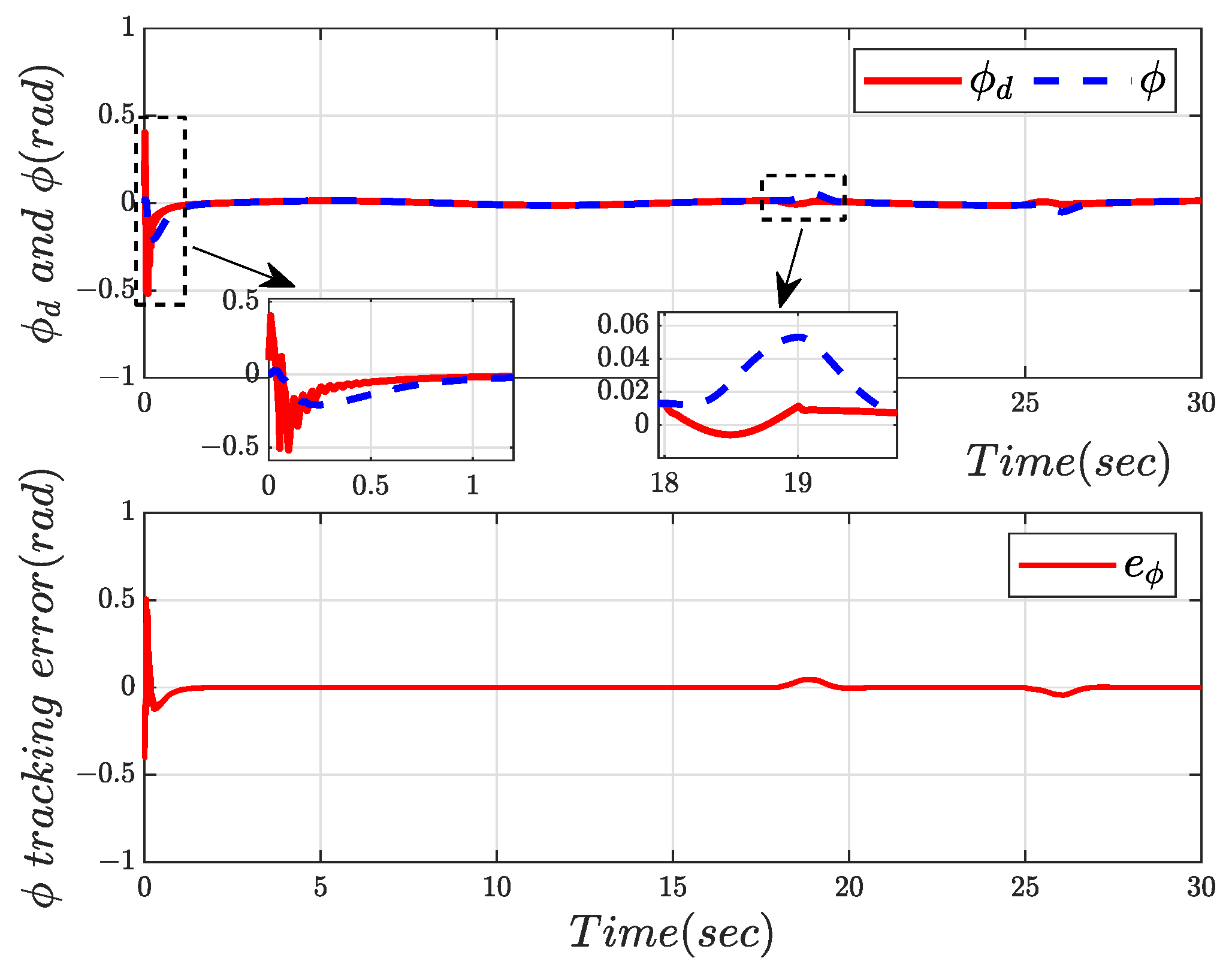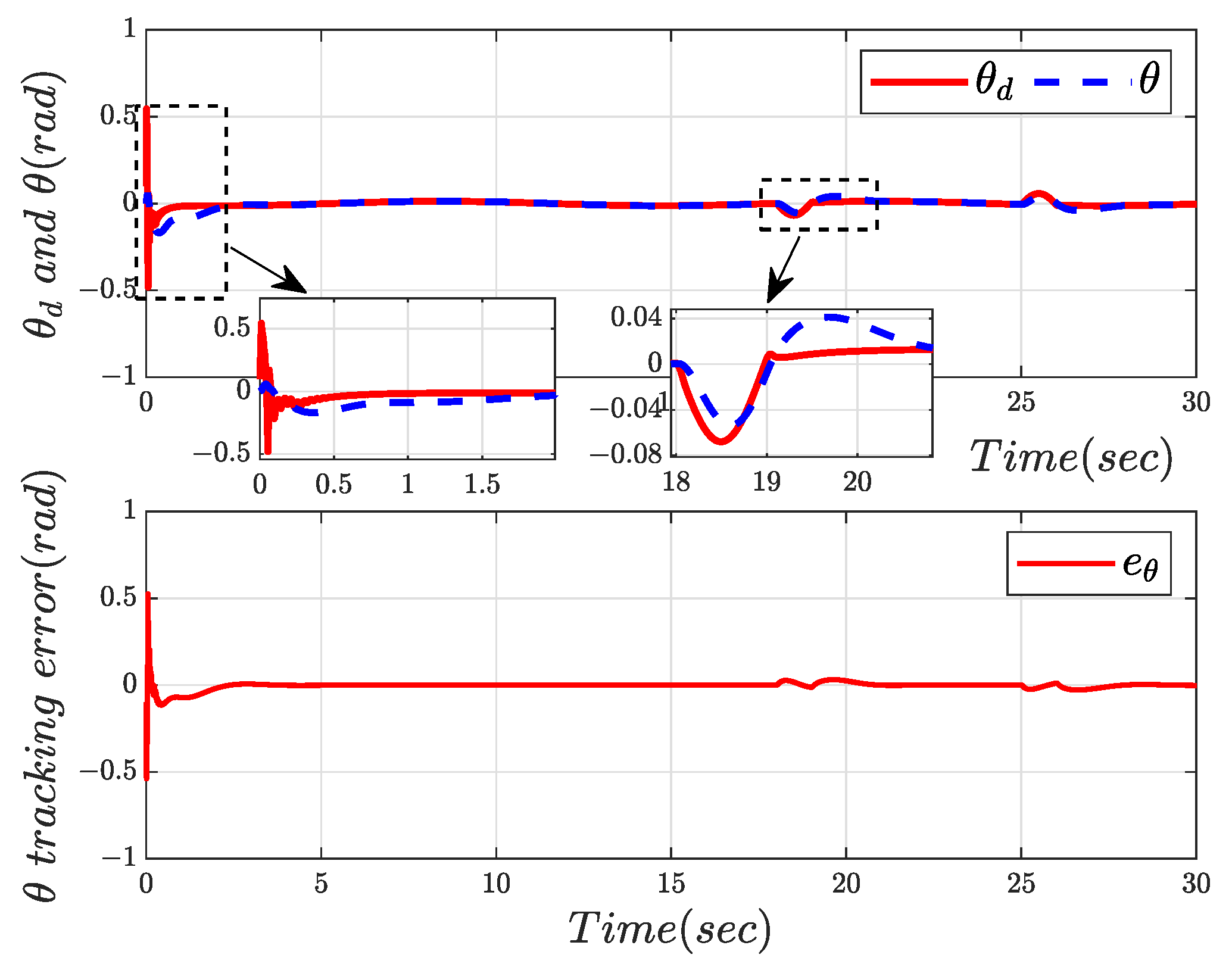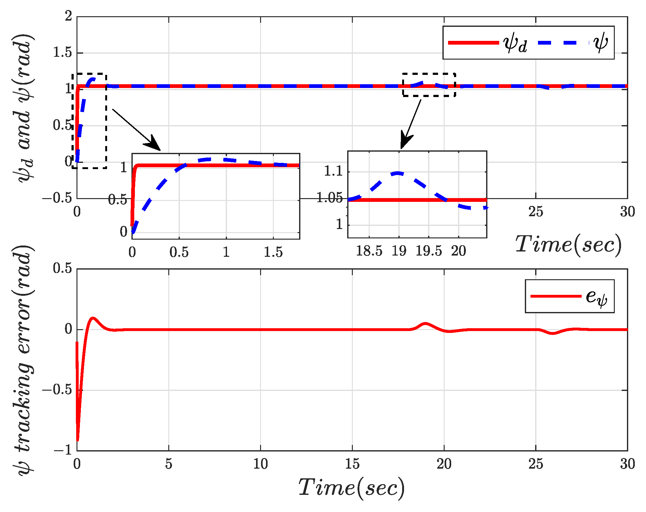Figure 11, Figure 12 and Figure 13 show the tracking and errors of the quadrotor’s roll, pitch, and yaw angles. In practical applications, large fluctuations in the roll and pitch angles are not allowed. The maximum roll angle in Figure 11 is less than 0.2 rad (approximately $11.{46}^{\circ }$), which is well within the permissible range. The maximum pitch and yaw angles in Figure 12 and Figure 13 are both less than 0.1 rad (approximately $5.{73}^{\circ }$), indicating very small oscillations in the Y and Z directions, and the deviations after disturbances at the 18th and 25th seconds are also very small (disturbance errors are within 0.1 rad). 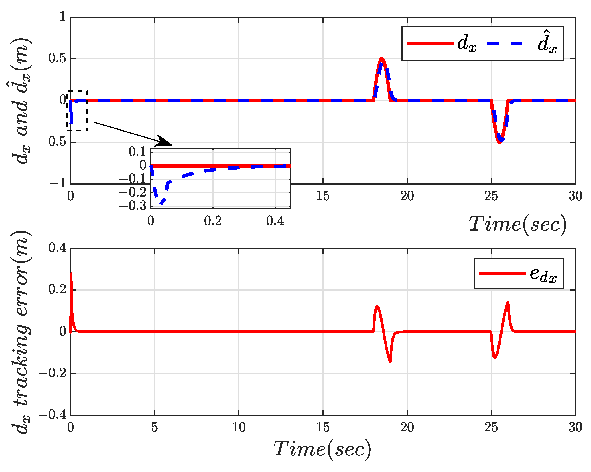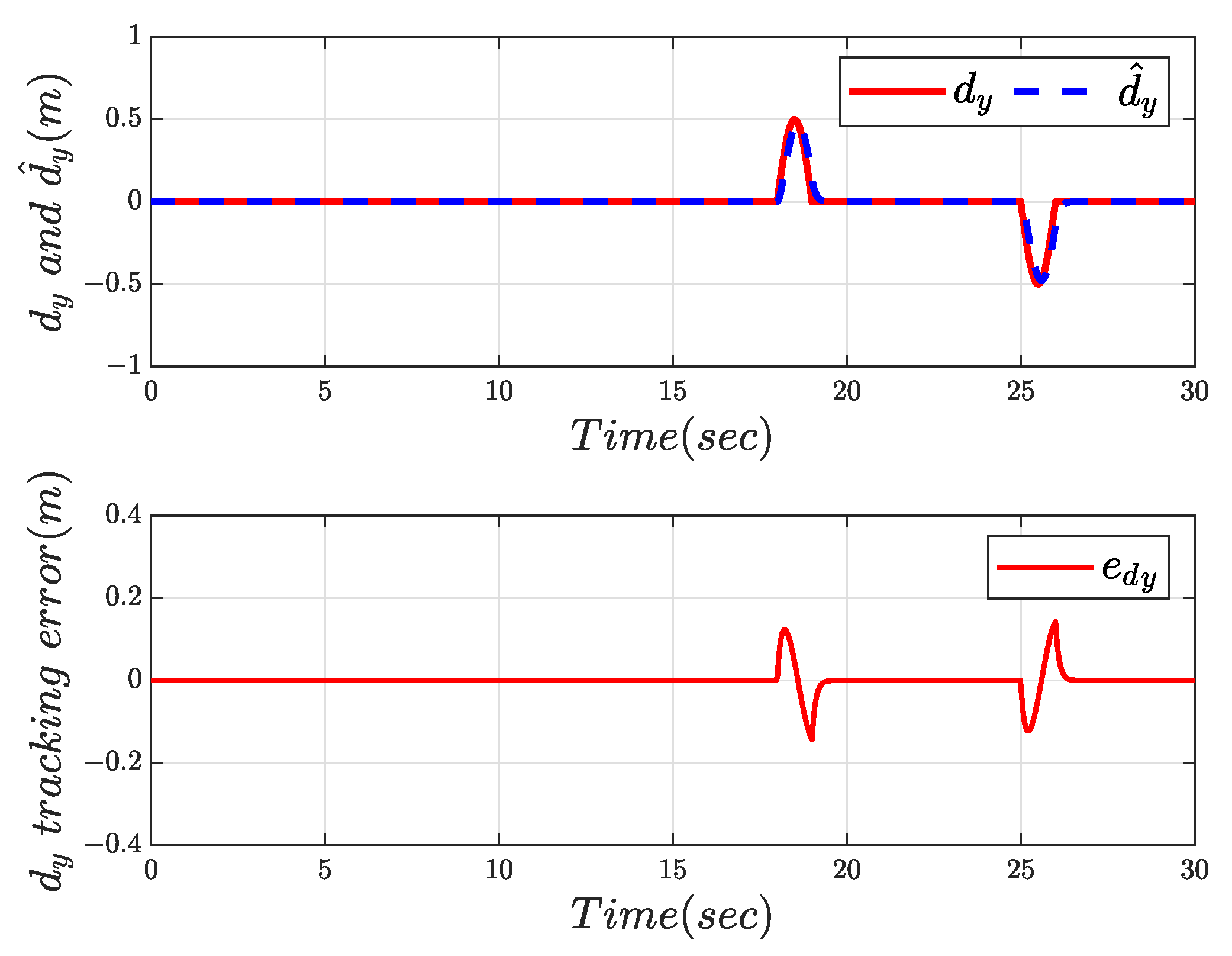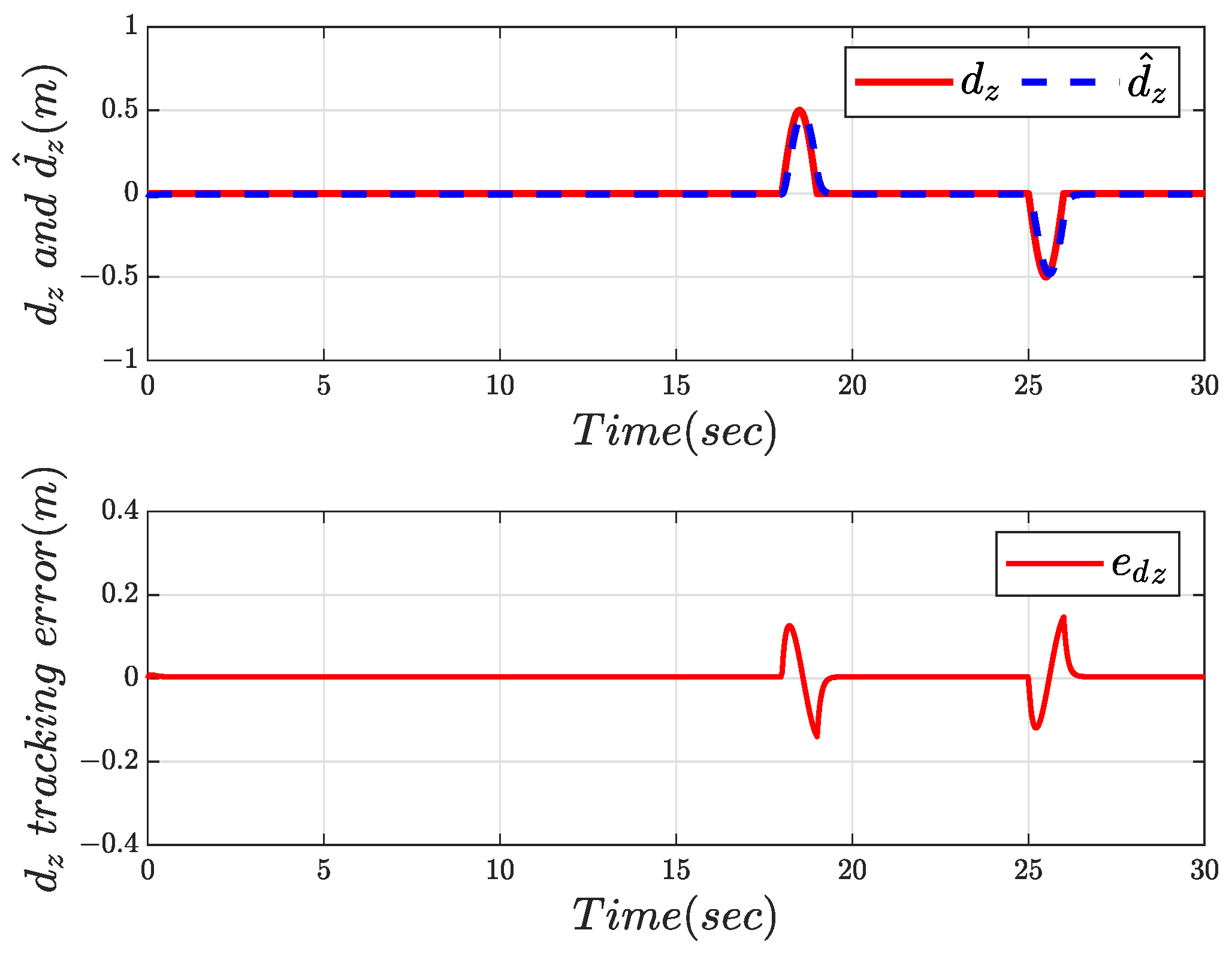Figure 14, Figure 15 and Figure 16 show the tracking and errors of disturbances in the X, Y, and Z directions. In Figure 14, there is an overshoot of about 0.3 m in the X direction during the initial 0.2 s. The Y and Z directions can track the external unknown disturbance signals well from the initial position, and the deviations after disturbances at the 18th and 25th seconds are also very small (tracking errors are within 0.1 m), indicating that the disturbance observer can effectively track external unknown disturbances. 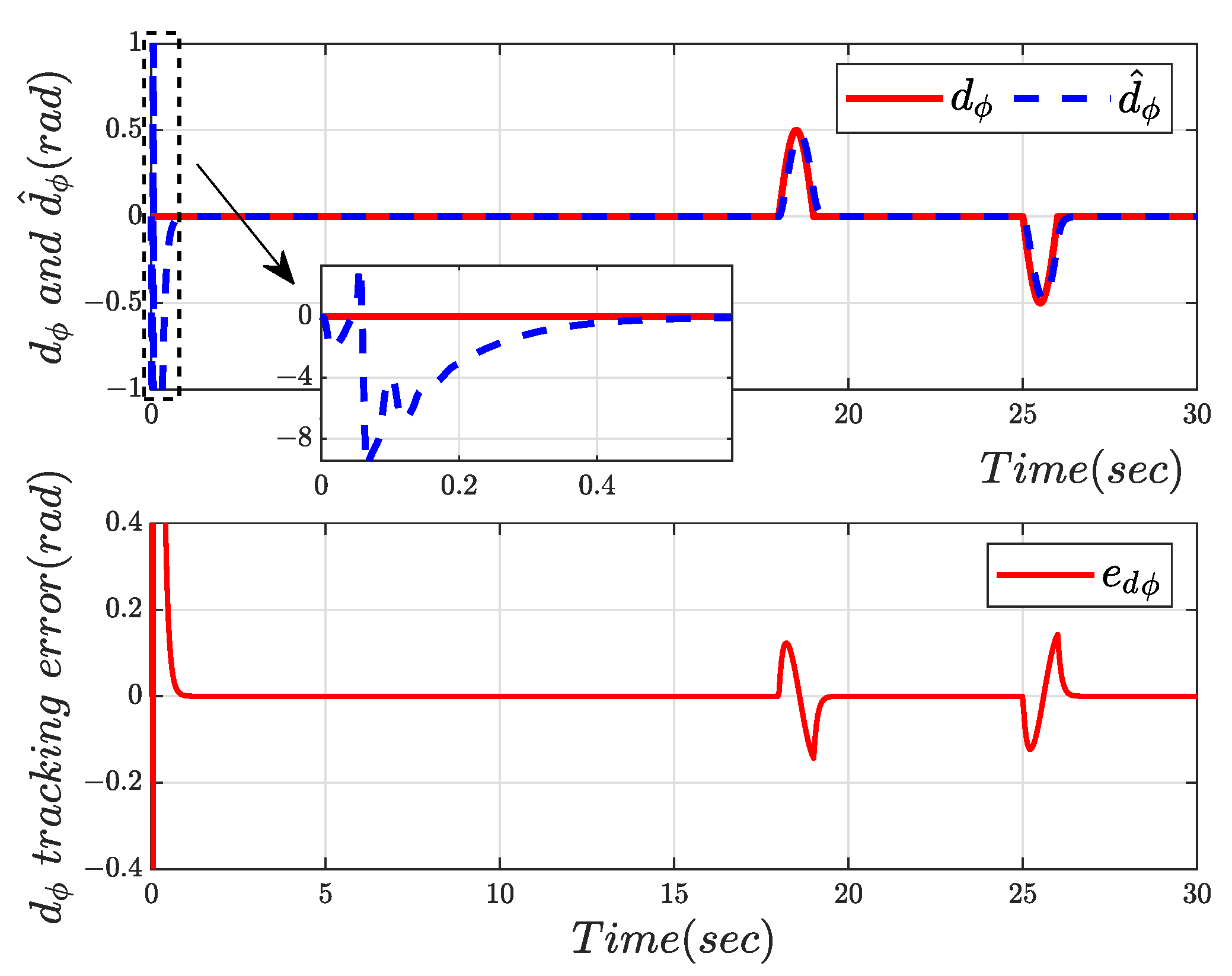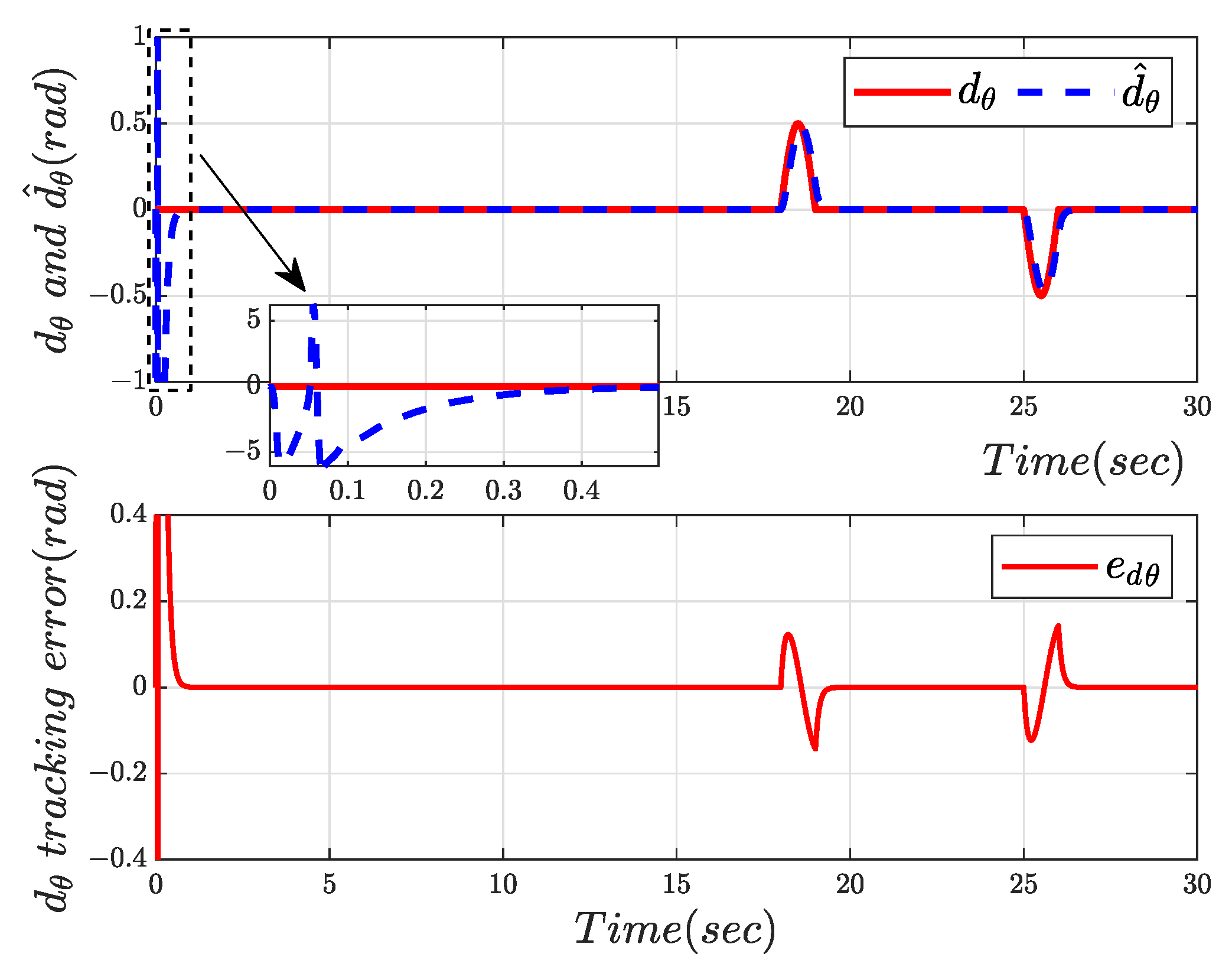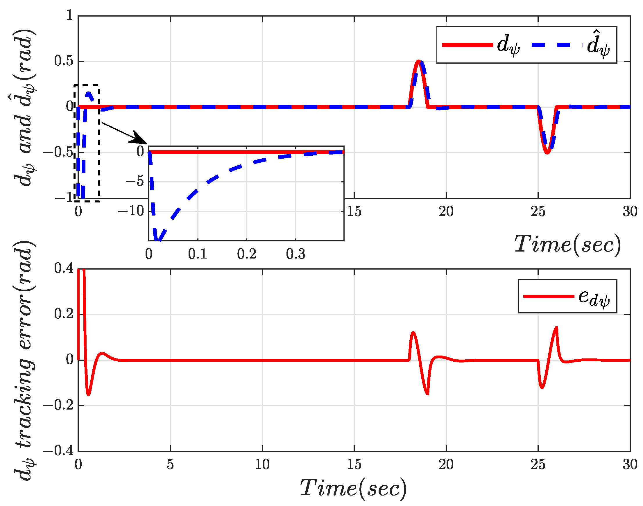Figure 17, Figure 18 and Figure 19 show the tracking and errors of disturbances in the roll, pitch, and yaw angles. Due to the presence of the attitude decoupler, the desired angle changes are large and fast, leading to significant initial overshoot in the disturbance observers for the roll, pitch, and yaw angles. However, after 0.4 s, they all track the external unknown disturbance signals, and the deviations after disturbances at the 18th and 25th seconds are also very small (tracking errors are within 0.1 rad), fully demonstrating that the designed observer can effectively track external unknown disturbances.

Experiment 2: The simulation results of DSC vs. NGACDOB

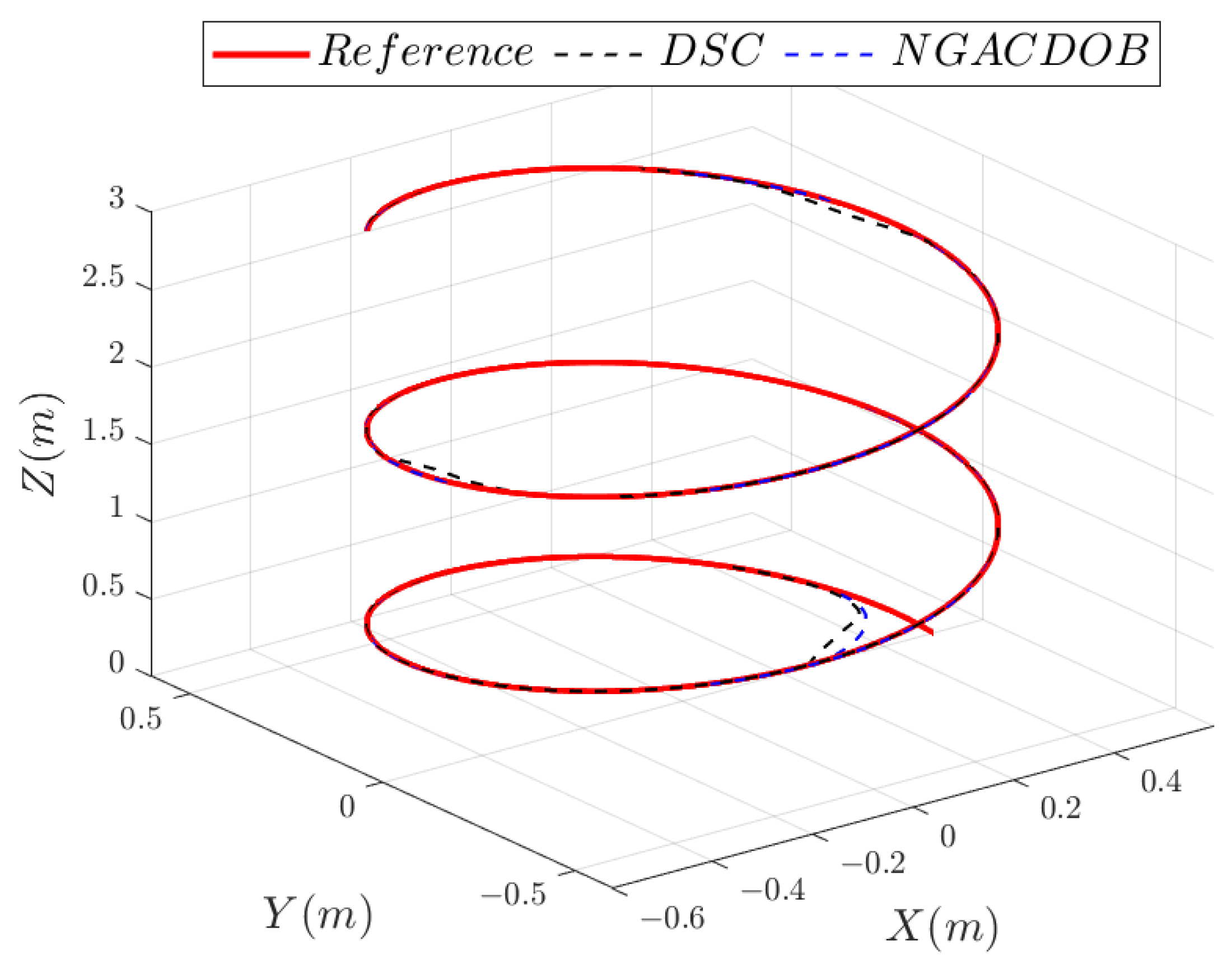
Figure 20 demonstrates the trajectory tracking performance of the DSC and NGACDOB controllers, where the blue line is able to track the red reference trajectory faster after the simulation starts, indicating that the NGACDOB controller has a faster response compared to the DSC controller. In Figure 21, the NGACDOB controller exhibits a faster response after the simulation begins, reaching steady-state at 0.6 s. When subjected to unknown external disturbances at the 18th and 25th seconds, the DSC controller shows a significant deviation, suggesting that the NGACDOB controller has better disturbance rejection performance. Figure 22 and Figure 23 show that the NGACDOB controller has a faster response and less overshoot in both the Y and Z directions, especially noticeable in the Z direction at the beginning. When disturbed at the 18th and 25th seconds, the NGACDOB controller demonstrates a much stronger disturbance rejection capability and a stronger recovery ability after the disturbance compared to the DSC controller.

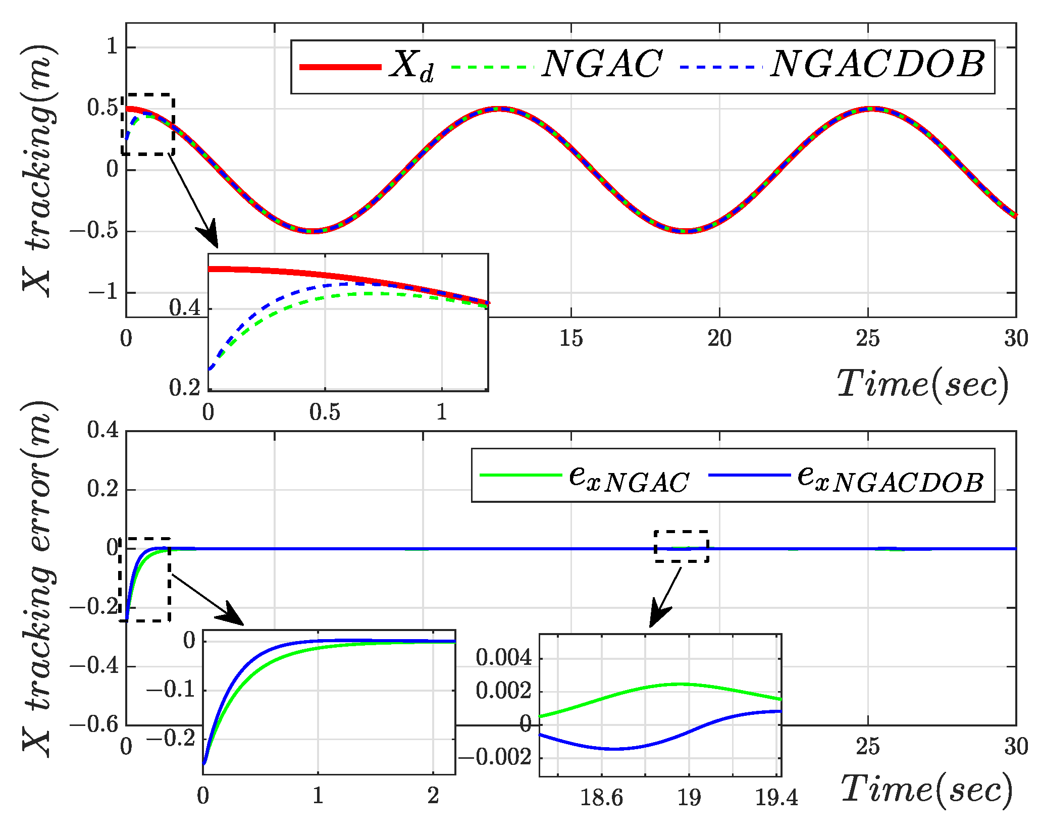
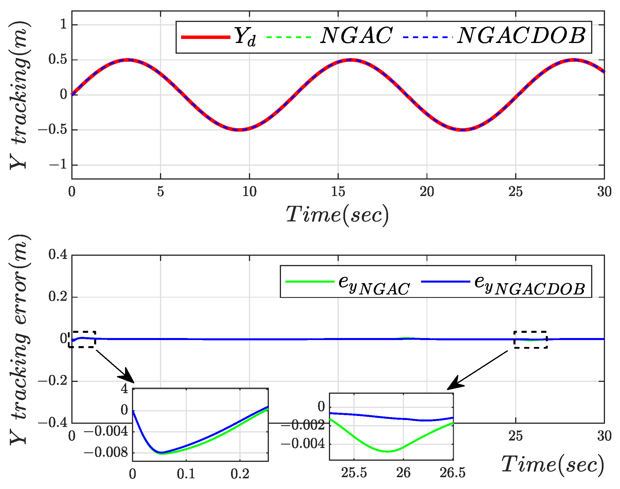
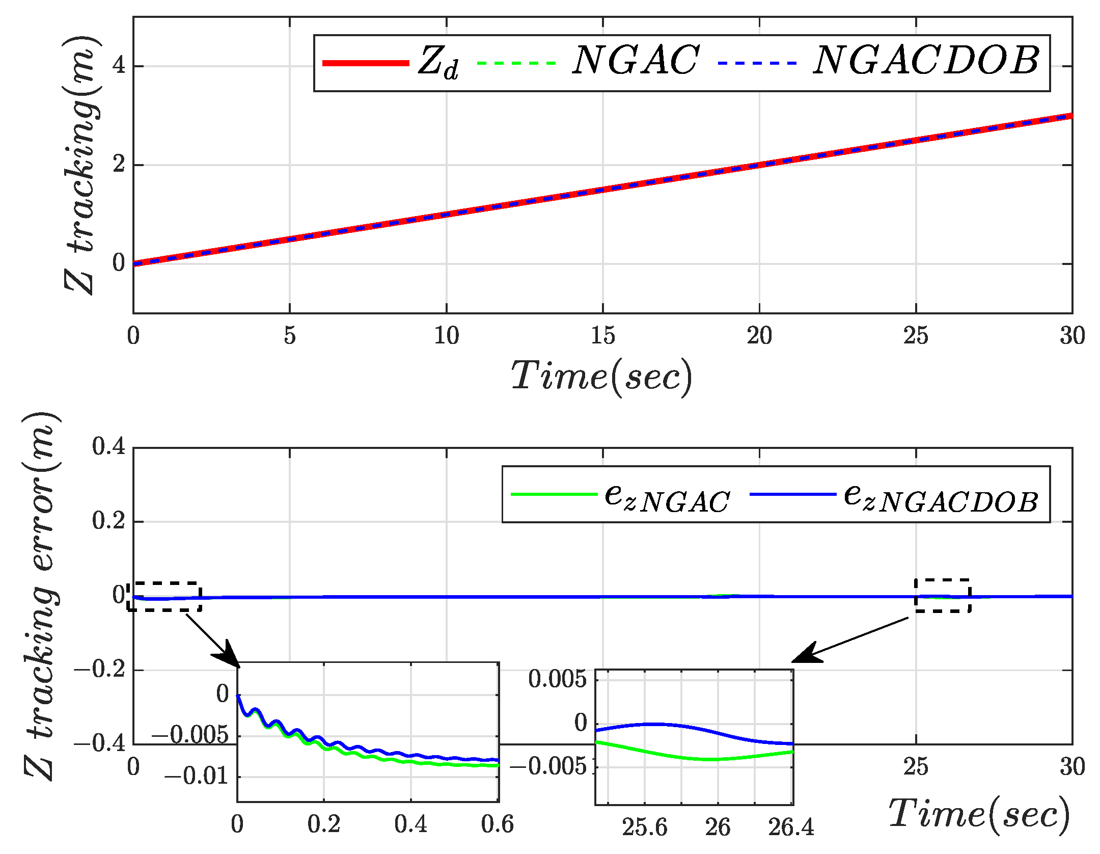
Experiment 3: The simulation results of NGAC vs. NGACDOB

The difference between the NGAC controller and the NGACDOB controller lies in the fact that the NGAC controller does not have a disturbance observer, and the impact of having or not having a disturbance observer can be seen in the experimental results. In Figure 24, the blue line shows a faster response, and at the 25th second, it is clear that the green line deviates from the red line, indicating that the NGACDOB controller has better disturbance rejection performance. Figure 25, Figure 26 and Figure 27 show that the NGACDOB controller has a faster response, but the advantage is not significant. When the system is disturbed at the 25th second, the difference in deviation between the two controllers in Figure 25 and Figure 27 is small, whereas the difference in Figure 26 is larger. Combining the four figures, it can be concluded that the NGACDOB controller has a slight advantage over the NGAC controller in terms of response speed and disturbance rejection capability.

5.4. Results Analysis

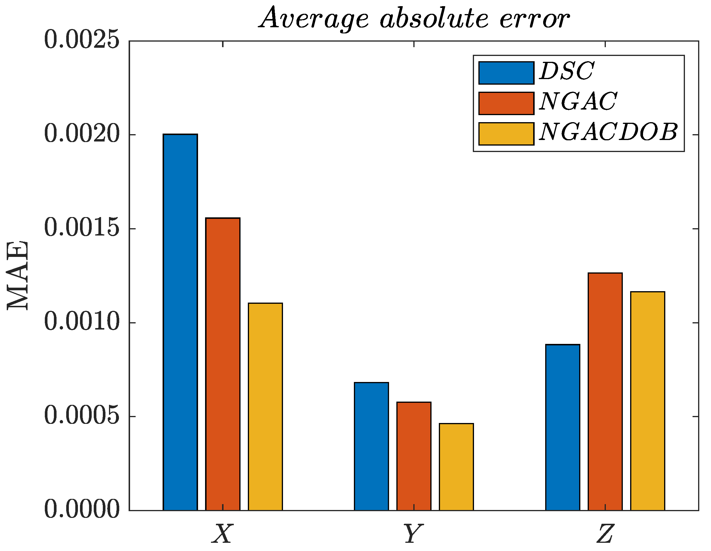
In this subsection, we analyze the data from the aforementioned experiments. To better analyze the tracking performance of different controllers, we employ two types of errors for a qualitative analysis of the three controllers discussed in the previous section.

The first error introduced is the Mean Absolute Error (MAE), which is a measure of the average magnitude of the errors between the reference values and the actual values. It is calculated by taking the absolute value of the difference between each pair of reference and actual values, summing these absolute differences, and then dividing by the number of data points. The formula for MAE is:

$$\begin{array}{c}\hfill \mathrm{MAE}=\frac{1}{n}\sum _{i=1}^n\left|y_i-{\widehat{y}}_i\right|\end{array}$$

(87)

where n is the number of data points, $y_i$ is the actual value of the i-th data point, ${\widehat{y}}_i$ is the reference value for the i-th data point. MAE is a non-negative value, and a lower MAE indicates a better fit of the model to the data, meaning the actual values are closer to the reference values.

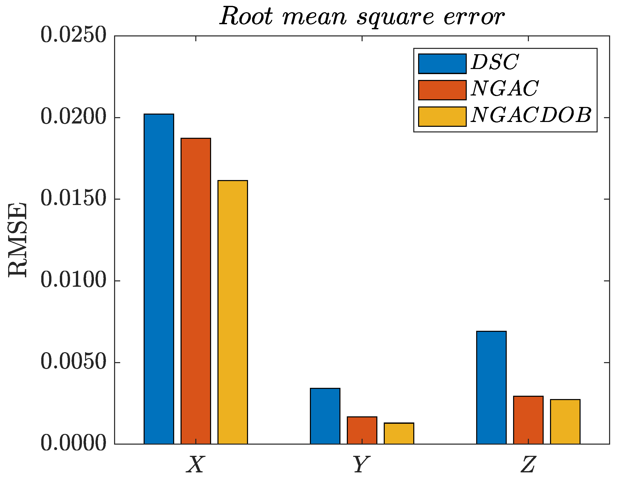
To better describe the stability of the controller, the second error introduced is the Root Mean Square Error (RMSE), which represents the standard deviation of the differences between reference values and actual values in a dataset. RMSE is calculated by squaring the differences between each reference value and the actual value, averaging these squared differences, and then taking the square root of the result. The formula for RMSE is:

$$\begin{array}{c}\hfill \mathrm{RMSE}=\sqrt{\frac{1}{n}\sum _{i=1}^n{(y_i-{\widehat{y}}_i)}^2}\end{array}$$

(88)

where n is the number of data points, $y_i$ is the actual value of the i-th data point, and ${\widehat{y}}_i$ is the reference value for the i-th data point. The value of RMSE reflects the degree of dispersion of actual values relative to reference values; a smaller RMSE indicates that the differences between actual and reference values are smaller, suggesting that the system is more stable.

Through the above two kinds of errors, the data of the three controllers in the above section are analyzed, and the comparison of data results is shown in Figure 28 and Figure 29.

Figure 28 presents the MAE comparisons among the three controllers, where the NGACDOB controller, compared to the DSC controller, reduces the error by 44.88% in the X direction, by 32.66% in the Y direction, and increases the error by 31.91% in the Z direction. When compared to the NGAC controller, the NGACDOB controller reduces the error by 29.09% in the X direction, by 19.72% in the Y direction, and by 7.90% in the Z direction. Therefore, the NGACDOB controller improves tracking in the X and Y directions but performs poorly in the Z direction. Figure 29 shows the RMSE comparisons among the three controllers, where the NGACDOB controller, compared to the DSC controller, reduces the error by 20.11% in the X direction, by 62.24% in the Y direction, and by 60.53% in the Z direction. When compared to the NGAC controller, the NGACDOB controller reduces the error by 13.78% in the X direction, by 22.80% in the Y direction, and by 6.99% in the Z direction. Thus, the NGACDOB controller exhibits better stability relative to the other two controllers.

6. Conclusions

In conclusion, this article presents an adaptive dynamic surface trajectory tracking control method employing a Nussbaum function for quadrotor UAVs facing unknown external disturbances and unidentified nonlinearities. The decomposition of the quadrotor dynamics model into two subsystems, focusing on position and attitude, expanded into six third-order subsystems, simplifies controller design expressions and enhances simulation program efficiency. The introduced adaptive controller based on Nussbaum gain effectively addresses actuator saturation, whereas a disturbance observer manages unknown disturbances within the system. Through hardware-in-the-loop experiments, conducted on the Rapid Control Prototype and Real-Time Simulator, the proposed control scheme demonstrates its effectiveness in trajectory tracking. These findings highlight the potential practical application of the proposed control method for quadrotor UAVs in uncertain environments.

References

1. Klosterman, S.; Melaas, E.; Wang, J.A.; Martinez, A.; Frederick, S.; O’Keefe, J.; Orwig, D.A.; Wang, Z.; Sun, Q.; Schaaf, C.; et al. Fine-scale perspectives on landscape phenology from unmanned aerial vehicle (UAV) photography. Agric. For. Meteorol. 2018, 248, 397–407. [Google Scholar] [CrossRef]
2. Fang, X.; Xie, L. Distributed Formation Maneuver Control Using Complex Laplacian. IEEE Trans. Autom. Control 2023. [Google Scholar] [CrossRef]
3. Fang, X.; Xie, L.; Li, X. Integrated relative-measurement-based network localization and formation maneuver control. IEEE Trans. Autom. Control 2023. [Google Scholar] [CrossRef]
4. Gao, J.; Hu, Z.; Bian, K.; Mao, X.; Song, L. AQ360: UAV-Aided Air Quality Monitoring by 360-Degree Aerial Panoramic Images in Urban Areas. IEEE Internet Things J. 2021, 8, 428–442. [Google Scholar] [CrossRef]
5. Zhang, H.; Dou, L.; Xin, B.; Chen, J.; Gan, M.; Ding, Y. Data Collection Task Planning of a Fixed-Wing Unmanned Aerial Vehicle in Forest Fire Monitoring. IEEE Access 2021, 9, 109847–109864. [Google Scholar] [CrossRef]
6. Huang, H.; Tang, Y.; Tan, Z.; Zhuang, J.; Hou, C.; Chen, W.; Ren, J. Object-Based Attention Mechanism for Color Calibration of UAV Remote Sensing Images in Precision Agriculture. IEEE Trans. Geosci. Remote Sens. 2022, 60, 4416013. [Google Scholar] [CrossRef]
7. Orfanus, D.; de Freitas, E.P.; Eliassen, F. Self-Organization as a Supporting Paradigm for Military UAV Relay Networks. IEEE Commun. Lett. 2016, 20, 804–807. [Google Scholar] [CrossRef]
8. Jia, N.; Yang, Z.; Yang, K. Operational Effectiveness Evaluation of the Swarming UAVs Combat System Based on a System Dynamics Model. IEEE Access 2019, 7, 25209–25224. [Google Scholar] [CrossRef]
9. Moreno-Valenzuela, J.; Pérez-Alcocer, R.; Guerrero-Medina, M.; Dzul, A. Nonlinear PID-Type Controller for Quadrotor Trajectory Tracking. IEEE/ASME Trans. Mechatron. 2018, 23, 2436–2447. [Google Scholar] [CrossRef]
10. Yoo, J.; Jang, D.; Kim, H.J.; Johansson, K.H. Hybrid Reinforcement Learning Control for a Micro Quadrotor Flight. IEEE Control Syst. Lett. 2021, 5, 505–510. [Google Scholar] [CrossRef]
11. Mofid, O.; Mobayen, S.; Wong, W.K. Adaptive Terminal Sliding Mode Control for Attitude and Position Tracking Control of Quadrotor UAVs in the Existence of External Disturbance. IEEE Access 2021, 9, 3428–3440. [Google Scholar] [CrossRef]
12. Huang, J.T.; Jiang, Y.W. Robust Adaptive Backstepping Control of Quadrotors With Unknown Input Gains. IEEE Access 2023, 11, 33069–33079. [Google Scholar] [CrossRef]
13. Liu, N.; Shao, X.; Yang, W. Integral Barrier Lyapunov Function Based Saturated Dynamic Surface Control for Vision-Based Quadrotors via Back-Stepping. IEEE Access 2018, 6, 63292–63304. [Google Scholar] [CrossRef]
14. Chen, Q.; Tao, M.; He, X.; Tao, L. Fuzzy Adaptive Nonsingular Fixed-Time Attitude Tracking Control of Quadrotor UAVs. IEEE Trans. Aerosp. Electron. Syst. 2021, 57, 2864–2877. [Google Scholar] [CrossRef]
15. Bisheban, M.; Lee, T. Geometric Adaptive Control With Neural Networks for a Quadrotor in Wind Fields. IEEE Trans. Control Syst. Technol. 2021, 29, 1533–1548. [Google Scholar] [CrossRef]
16. Imran, I.H.; Stolkin, R.; Montazeri, A. Adaptive Control of Quadrotor Unmanned Aerial Vehicle With Time-Varying Uncertainties. IEEE Access 2023, 11, 19710–19724. [Google Scholar] [CrossRef]
17. Lopez-Sanchez, I.; Moreno-Valenzuela, J. PID control of quadrotor UAVs: A survey. Annu. Rev. Control 2023, 56, 100900. [Google Scholar] [CrossRef]
18. Besnard, L.; Shtessel, Y.B.; Landrum, B. Quadrotor vehicle control via sliding mode controller driven by sliding mode disturbance observer. J. Frankl. Inst. 2012, 349, 658–684. [Google Scholar] [CrossRef]
19. Almakhles, D.J. Robust Backstepping Sliding Mode Control for a Quadrotor Trajectory Tracking Application. IEEE Access 2020, 8, 5515–5525. [Google Scholar] [CrossRef]
20. Razmi, H.; Afshinfar, S. Neural network-based adaptive sliding mode control design for position and attitude control of a quadrotor UAV. Aerosp. Sci. Technol. 2019, 91, 12–27. [Google Scholar] [CrossRef]
21. Raffo, G.V.; Ortega, M.G.; Rubio, F.R. An integral predictive/nonlinear H∞ control structure for a quadrotor helicopter. Automatica 2010, 46, 29–39. [Google Scholar] [CrossRef]
22. Zhang, X.; Wang, Y.; Zhu, G.; Chen, X.; Li, Z.; Wang, C.; Su, C.Y. Compound Adaptive Fuzzy Quantized Control for Quadrotor and Its Experimental Verification. IEEE Trans. Cybern. 2021, 51, 1121–1133. [Google Scholar] [CrossRef]
23. Cohen, M.R.; Abdulrahim, K.; Forbes, J.R. Finite-Horizon LQR Control of Quadrotors on SE2(3). IEEE Robot. Autom. Lett. 2020, 5, 5748–5755. [Google Scholar] [CrossRef]
24. Chen, H.; Zhou, J.; Zhou, M.; Zhao, B. Nussbaum gain adaptive control scheme for moving mass reentry hypersonic vehicle with actuator saturation. Aerosp. Sci. Technol. 2019, 91, 357–371. [Google Scholar] [CrossRef]
25. Wen, C.; Zhou, J.; Liu, Z.; Su, H. Robust adaptive control of uncertain nonlinear systems in the presence of input saturation and external disturbance. IEEE Trans. Autom. Control 2011, 56, 1672–1678. [Google Scholar] [CrossRef]
26. Zhang, G.; Dong, X.; Liu, J.; Zhang, X. Nussbaum-type function based robust neural event-triggered control of unmanned surface vehicle subject to cyber and physical attacks. Ocean Eng. 2023, 270, 113664. [Google Scholar] [CrossRef]
27. Chen, F.; Jiang, R.; Zhang, K.; Jiang, B.; Tao, G. Robust backstepping sliding-mode control and observer-based fault estimation for a quadrotor UAV. IEEE Trans. Ind. Electron. 2016, 63, 5044–5056. [Google Scholar] [CrossRef]
28. Kim, J.; Kang, M.S.; Park, S. Accurate modeling and robust hovering control for a quad-rotor VTOL aircraft. In Selected Papers from the 2nd International Symposium on UAVs, Reno, NV, USA, 8–10 June 2009; Springer: Berlin/Heidelberg, Germany, 2010; pp. 9–26. [Google Scholar]
29. Nussbaum, R.D. Some remarks on a conjecture in parameter adaptive control. Syst. Control Lett. 1983, 3, 243–246. [Google Scholar] [CrossRef]
30. Khalil, H.; Grizzle, J. Nonlinear Systems, 2nd ed.; Prentice Hall: Upper Saddle River, NJ, USA, 1996. [Google Scholar]
31. Gao, Z.; Ding, L.; Zheng, X. Attitude control for a quadrotor based on nonlinear disturbance observer. J. Electron. Meas. Instrum. 2019, 33, 427–435. [Google Scholar]
32. Yang, J.; Li, S.; Yu, X. Sliding-Mode Control for Systems With Mismatched Uncertainties via a Disturbance Observer. IEEE Trans. Ind. Electron. 2013, 60, 160–169. [Google Scholar] [CrossRef]
33. Yu, Z.; Zhang, Y.; Jiang, B.; Su, C.Y.; Fu, J.; Jin, Y.; Chai, T. Nussbaum-based finite-time fractional-order backstepping fault-tolerant flight control of fixed-wing UAV against input saturation with hardware-in-the-loop validation. Mech. Syst. Signal Process. 2021, 153, 107406. [Google Scholar] [CrossRef]
34. Zhang, Y.; Xu, N.; Zhu, G.; Sun, L.; Cao, S.; Zhang, X. Adaptive robust dynamic surface integral sliding mode control for quadrotor UAVs under parametric uncertainties and external disturbances. Complexity 2020, 2020, 8879364. [Google Scholar] [CrossRef]
Figure 1. Quadrotor UAV structure diagram.
Drones 08 00077 g001
Figure 2. Quadrotor UAV control system.
Drones 08 00077 g002
Figure 3. The block diagram of the quadrotor UAV control scheme.
Drones 08 00077 g003
Figure 4. The diagram of Modeling Tech experimental platform.
Drones 08 00077 g004
Figure 5. Hardware structure diagram of experiment platform.
Drones 08 00077 g005
Figure 6. A 3D trajectory tracking diagram of quadrotor UAVs.
Drones 08 00077 g006
Figure 7. Quadrotor UAV input state changes.
Drones 08 00077 g007
Figure 8. Tracking and error in X-direction.
Drones 08 00077 g008
Figure 9. Tracking and error in Y-direction.
Drones 08 00077 g009
Figure 10. Tracking and error in Z-direction.
Drones 08 00077 g010
Figure 11. Roll angle tracking and error.
Drones 08 00077 g011
Figure 12. Pitch angle tracking and error.
Drones 08 00077 g012
Figure 13. Yaw angle tracking and error.
Drones 08 00077 g013
Figure 14. Disturbance tracking and error in X-direction.
Drones 08 00077 g014
Figure 15. Disturbance tracking and error in Y-direction.
Drones 08 00077 g015
Figure 16. Disturbance tracking and error in Z-direction.
Drones 08 00077 g016
Figure 17. Roll angle disturbance tracking and error.
Drones 08 00077 g017
Figure 18. Pitch angle disturbance tracking and error.
Drones 08 00077 g018
Figure 19. Yaw angle disturbance tracking and error.
Drones 08 00077 g019
Figure 20. DSC and NGACDOB trajectory tracking.
Drones 08 00077 g020
Figure 21. Tracking and errors of DSC and NGACDOB in X-direction.
Drones 08 00077 g021
Figure 22. Tracking and errors of DSC and NGACDOB in Y-direction.
Drones 08 00077 g022
Figure 23. Tracking and errors of DSC and NGACDOB in Z-direction.
Drones 08 00077 g023
Figure 24. NGAC and NGACDOB trajectory tracking.
Drones 08 00077 g024
Figure 25. Tracking and errors of NGAC and NGACDOB in X-direction.
Drones 08 00077 g025
Figure 26. Tracking and errors of NGAC and NGACDOB in Y-direction.
Drones 08 00077 g026
Figure 27. Tracking and errors of NGAC and NGACDOB in Z-direction.
Drones 08 00077 g027
Figure 28. Average absolute error.
Drones 08 00077 g028
Figure 29. Root mean square error.
Drones 08 00077 g029